Modeling and Application of Customer Lifetime Value in Online Retail


1
Department of Information Technologies, Faculty of Informatics and Statistics, University of Economics, Prague, W. Churchill Sq. 1938/4, 130 67 Prague, Czech Republic
2
Department of Statistics and Probability, Faculty of Informatics and Statistics, University of Economics, Prague, W. Churchill Sq. 1938/4, 130 67 Prague, Czech Republic
3
Department of Systems Analysis, Faculty of Informatics and Statistics, University of Economics, Prague, W. Churchill Sq. 1938/4, 130 67 Prague, Czech Republic
4
Department of Software Engineering, Faculty of Nuclear Sciences and Physical Engineering, Czech Technical University in Prague, Brehova 7, 115 19 Prague 1, Czech Republic
*
Author to whom correspondence should be addressed.
Informatics 2018, 5(1), 2; https://doi.org/10.3390/informatics5010002
Submission received: 11 December 2017
/
Revised: 31 December 2017
/
Accepted: 3 January 2018
/
Published: 6 January 2018
Abstract
:This article provides an empirical statistical analysis and discussion of the predictive abilities of selected customer lifetime value (CLV) models that could be used in online shopping within e-commerce business settings. The comparison of CLV predictive abilities, using selected evaluation metrics, is made on selected CLV models: Extended Pareto/NBD model (EP/NBD), Markov chain model and Status Quo model. The article uses six online store datasets with annual revenues in the order of tens of millions of euros for the comparison. The EP/NBD model has outperformed other selected models in a majority of evaluation metrics and can be considered good and stable for non-contractual relations in online shopping. The implications for the deployment of selected CLV models in practice, as well as suggestions for future research, are also discussed.
1. Introduction
The segmentation of customers according to their customer lifetime value (CLV) enables companies to adequately build long-term relationships with customers and effectively manage investments into marketing tools. CLV contributes to solving a number of problems such as decisions related to addressing, retaining and acquiring customers, or issues concerning a company’s long-term value [1]. Many different CLV models were devised in recent decades and, at the same time, the development of ICT gave rise to e-commerce, which is a fast-growing retail market in Europe and the USA [2]. The important part of e-commerce is online shopping, which offers retail sales directly to consumers. Companies engaged in e-commerce have high data availability due to the interactions of customers with their websites and other Internet-based services. The high level of competition, especially in online shopping, drives companies to spend their financial resources on marketing activities as efficiently as possible, which can be helped by implementing a CLV model that uses available historical data to estimate customer value. However, in their effort to introduce CLV as a decision-making basis for marketing management, companies operating an online store face the issue of selecting the appropriate CLV model that would be suitable for their kind of business.
The aim of this article is to empirically compare the predictive ability and quality of selected CLV models used in the online shopping environment on the basis of statistical metrics. In addition, the article has a practically oriented aim: to help companies involved in online shopping make a decision concerning the selection and the application of the selected CLV model. Other recommendations concerning the implementation of a particular model are also introduced. Based on managerial issues, this article proposes one research question:
Which of the compared models for calculating CLV has a good predictive performance of CLV in the non-contractual environment of e-commerce?
Good predictive performance is observed when stable quality prediction results can be achieved among all used datasets based on evaluation metrics, and outperform the other compared models in this study. An implicit restriction is the number of different models selected for comparison, see Section 3.1. On the other hand, the selected models represent very different approaches to CLV modeling, as shown below.
There are two main reasons for performing such research. Firstly, there exist a significant number of reviews comparing the theoretical aspects of selected CLV models based on results from secondary sources, e.g., [3,4,5,6,7,8,9,10,11]. However, very few of the comparative papers are directly based on original empirical research creating a connection between the theoretical and the practical level, which means applying given models to a specific area. There are only two examples of this type of comparative paper [12,13]. It is evident that in terms of creating a connection between the theoretical and the practical level the situation is unsatisfactory. This was the principal reason for the authors to carry out their own wider comparative study of selected CLV models that could be used in the field of e-commerce, including online shopping.
The second reason for performing this study is methodological. This need for empirical comparison of models is based on the fact that the CLV applies, in particular, design science research. The research methodology thus builds on the principles applied in design science [14,15]. Design science designs and investigates artifacts (e.g., models) that can be regularly tested in different contextual conditions, and thus generates a knowledge base that will affect any similar artifacts in the future. This knowledge also helps to theorize in the area [15,16]. Therefore, this article is a complementary addition to artifact design, which is involved in the evaluation and comparison based on real-world data used by the selected models. The need for such research emphasizes even articles from the marketing area, e.g., [3,11,17,18], and even methodological articles dealing with design science research e.g., [14,16,19]. For other theoretically oriented and review articles, such research brings the following types of benefits:
- Better comparable results of the deployment of selected models. Theoretically orientated studies build on secondary sources, most often on the results of the validation of the proposed model in the original article. The problem with studies built on secondary sources rather than comparative empirical research is that the conclusions about the behavior of a model and its comparison with another model are based on the use of entirely different datasets and conditions. This brings up the issue of relevant generalizations based on different results.
- New findings for the empirical process of building an information base on individual models. For example, Gupta et al. [11] consider persistence models, e.g., the Vector Autoregressive model (VAR), as very appropriate for CLV calculation; however, they add that there are very few examples using these models because the demands for data are high. Only the introduction of other applications, for example particular model to new datasets, can enhance the debate about the appropriateness or limits of a particular model in comparison to others, and extend it further by a discussion about the areas of usability.
Up to now only comparisons of a larger number of selected models in one dataset [12,13] have been performed, allowing a comparison of results, but also limiting the generalization of results achieved beyond the dataset. In this regard, the presented article is unique because it offers a comparison of the models on six large datasets of selected online stores. The EP/NBD and MC models selected for this study are based on different approaches to modeling. According to [11] these models are classified as probability and econometric approaches to modeling CLV. Furthermore, compared to the studies [12,13], this article offers a different view based on the non-contractual relation typical of online shopping as a part of e-commerce business.
This article connects the theoretical and the practical level by discussing the results acquired from the comparative analysis, which can help companies arrive at a decision on selecting the CLV model suitable for their online shopping conditions, and implement that model. The reliability of the selected CLV models is empirically compared using six datasets from medium to large Czech and Slovak online stores. The results of the comparison are used as the basis for a discussion of individual models, their suitability, and managerial and implementation aspects in the sense of their robustness and accuracy of prediction. As a result, companies running medium- and large-sized e-commerce will not need to carry out their own extensive experiments with different CLV models. That was also the practical motivation for this article because the online shopping industry lacks more extensive comparative analyses of CLV models carried out on up-to-date empirical data using more than one dataset.
The article is structured in the following way: Section 2 introduces the theoretical basis of CLV. An explorative analysis of the datasets used, as well as the method of carrying out a comparative analysis of selected CLV models, can be found in Section 3. This section also mentions the selection of CLV models for comparison and an examination of relevant literature concerning the selected models. The results obtained from the comparative analysis are presented in Section 4 and then discussed in Section 5.
2. Background
Customers are central to all marketing activities of a company because not only do they generate income, but they increase the company’s market value as well. Marketing emphasizes the interconnection of all processes and activities that create, communicate and provide values for customers, including customer relationship management [20].
In the past two decades, the field of customer relationship management (CRM) went through a significant transformation thanks to information and communication technologies (mainly database and analytical technology). When analyzing customer feedback, companies no longer have to rely only on the aggregated results of quantitative and qualitative research (e.g., questionnaires, focus groups), but they can use their own customer data and concentrate on selected groups or individual customers. This was achieved thanks to the new possibilities of storing and processing available data about individual customers.
This progress enabled a departure from the established patterns, such as brand equity, transaction and product centricity, and a shift towards a customer-centric approach in relationship management [21,22], in which the customer is a valuable intangible asset of the company [23,24,25,26]. The aim of CRM activities is mainly to retain current customers, build a long-term relationship, and gain new customers [27]. The CLV approach plays an important role in that process, as it enables companies to segment customers and identifies those who bring the company the largest profit in time [28]. Concurrently, it makes it possible to choose suitable strategies for activities within the company’s CRM.
There is a number of slightly different definitions of CLV, see the comparison of definitions in articles [7,29,30]. A generally accepted definition of CLV is the present value of future net cash flows [31] associated with a particular customer [22].
Companies also use other indicators, such as Customer Profitability (CP). CP refers to the revenues, minus the costs connected to maintaining a mutual relationship, generated during a selected period [31,32,33]. In other words, this is a contemporary or retrospective view [3] as opposed to CLV, which offers a look ahead. For this reason, the use of CLV is more suitable (better than the historical CP analysis) for strategic and tactical marketing planning [3,7,32,34].
The CLV approach forms a bridge between marketing and financial metrics, which means that marketing activities are always related to financial metrics, allowing space for optimization and management [35]. CLV shows the way in which (changes in) customer behavior (e.g., increased purchase, retention) can influence future profitability [6]. The relevancy of CLV applications is leveraged mainly by customer behavior impacting retention [36], customer-level attributes impacting customer loyalty (e.g., age and gender) [37], and national cultural dimensions affecting the drivers of purchase, frequency and contribution margin [17]. All of these (and other) components used for appropriate CLV models with available data constitute both direct and indirect influences on CLV calculations. The main researched applications of CLV are aimed at the business-to-consumer context while the business-to-business applications are focused on customer asset management [38].
Closely connected to CLV is the Customer Equity (CE) indicator, which is used mainly for calculating a company’s long-term value. That is usually defined as the sum of the CLV of all current customers of the company [22], or it can be the sum of the CLV of all current and potential customers [39,40,41,42]. In this article, CE will be understood according to [22] above, but for the sake of completeness, it should be added that earlier articles, in particular, understand CE also as the average CLV minus acquisition costs [43,44]. Unlike CLV, this definition takes acquisition costs into account [7].
The past three decades saw the introduction of a vast number of different models and approaches to calculating CLV designed for various types of companies, businesses or chosen management views. One of the possible and often mentioned divisions of CLV models according to the customer-company relationship is into contractual relations (lost for good, retention), semi-contractual relations and non-contractual relations (always a share, migration) [7].
Within the literature were found only two studies in the Web of Science, which include a greater number of comparisons of selected models for the calculation of CLV based on their empirical research, and therefore a comparison of the predictive capabilities of selected CLV models on a single dataset on the basis of statistical metrics. Donkers et al. [12] analyzed a dataset from an insurance company with contractual settings and concluded that simple profit regression models achieve the best performance. Batislam et al. [13] used a dataset from a grocery retailer repeatedly focusing on store cards and their usage as the drivers of higher purchase frequency by customers. The results confirm the better performance of their own modified Beta Geometric/NBD model (BG/NBD) customized to the specified business settings in comparison with Pareto/NBD and original BG/NBD models. It can be stated that even simple models achieve excellent prediction results despite the more complex models being expected to capture the depth of relationship developments better. Similarly, it can be expected that modified models or those designed for specific conditions and environment will produce better predictions in relevant cases than more complex, universally applicable models (achieving consistently good results in various situations).
This article focuses on non-contractual relations typical for e-commerce companies engaged in online shopping. Such companies usually have at their disposal an extensive database concerning their customers, which they use for internal purposes (e.g., financial management, marketing). This kind of online retail market, focusing on selling to end customers, has been growing continuously and it can thus be expected that the number of Internet-based services such as online stores will increase. The same applies to the competitive pressure put on them. In Europe alone, estimated total online sales in Europe in 2016 grew to €530 billion by 15.4% compared to 2015 [45], with much room for improvement as only 18% of companies are selling online. Every online shopper in Europe was expected to spend $1330 in 2015 compared to $1816 in the USA [45], for a comparison see also other surveys [45,46]. The focus on e-commerce companies engaged in online shopping is therefore very topical both in local and global context.
3. Methodology and Data Collection
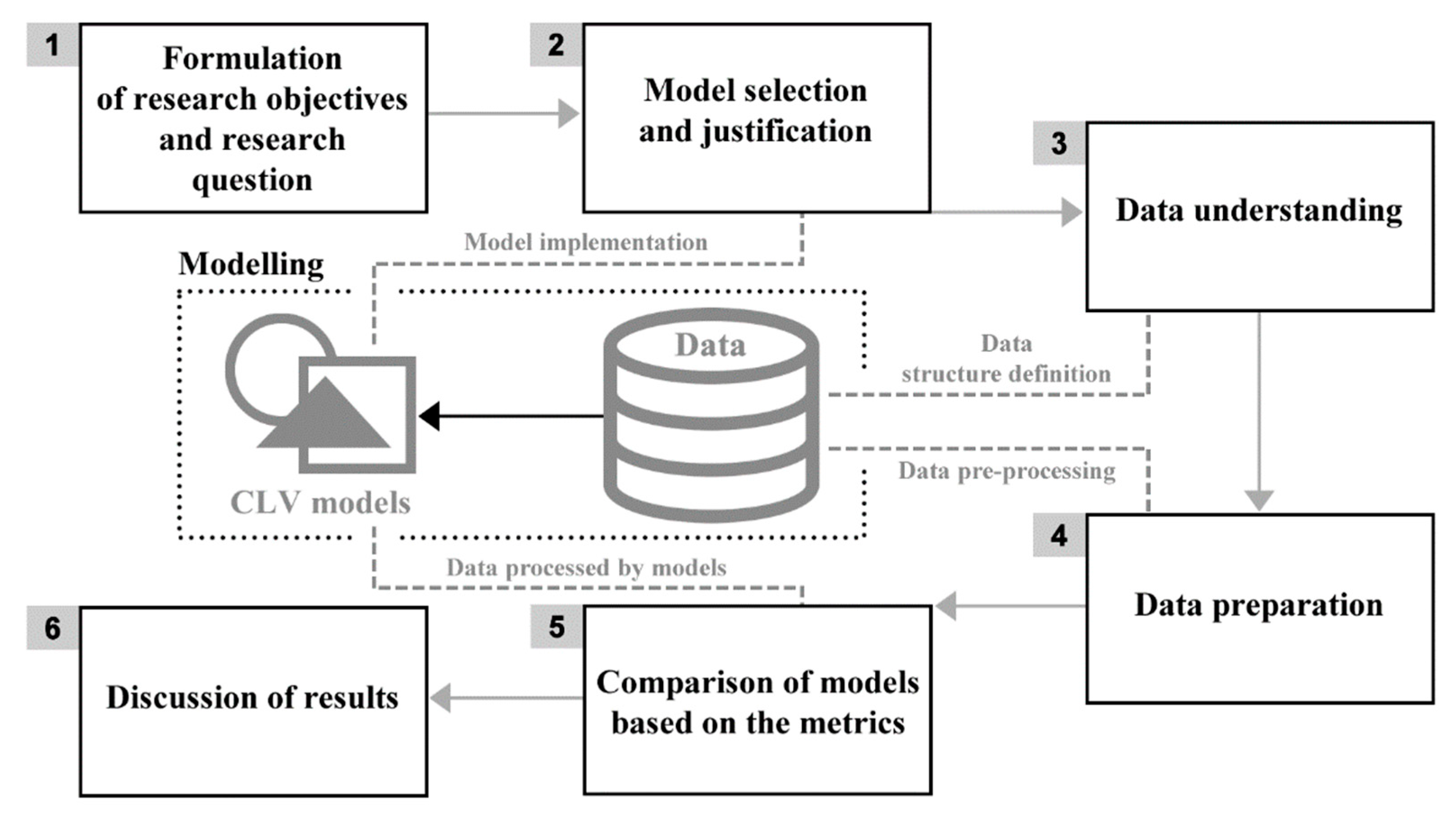
The research methodology consists of six phases, which are illustrated in Figure 1. The initial phase of the research set the research objectives and formulated the research question. It also justified the need and appropriateness of the proposed research, see Section 1 and Section 2. The second phase included the selection and justification of choice of CLV models suitable for use by e-commerce companies engaged in online shopping. In this stage, the implementation of the selected models was also performed according to the described models set out in Section 3.1. In the third phase, data requirements were defined, based on the selected models. On this basis, it was possible to determine what data, in what form and for what period will be needed in order to perform the research, see Section 3.2. In the fourth phase, data was collected from various e-commerce companies in the required structure. Further, the acquired datasets that met the specified requirements were pre-processed for the needs of the individual models. The data pre-processing is described in Section 3.2. Section 3.3 describes the datasets from various e-commerce companies.
The fifth phase of the research compared the selected CLV models based on statistical metrics listed in Section 3.4. This section also describes how to perform the comparison, including the definition of a training and testing period. In the last, sixth phase of the research, the research question is answered first in Section 4, and then the obtained results are subjected to a wider discussion including relevant managerial implications in Section 5.
3.1. Selection of Models for Comparison and Their Description
Gupta et al. [11] presents six different modeling approaches: RFM, probability, econometric, persistence, computer science and diffusion/growth models. In this study, probability and econometric models were selected, as they are suitable for online shopping conditions in the e-commerce business. For the comparison, previously published models were selected: Extended Pareto/NBD [47] as one of the probability models with RFM factors used in its computations and the Markov chain model [48,49] as one of the econometric models. Computer science models were excluded from this study because they are very little mentioned in the literature focused on CLV calculation. Finally, diffusion/growth [11] and persistence models (e.g., VAR model) [50] were not included because the models are not usable at the level of individual customers prediction and they are more used to calculating CE.
Although it was viable to select even more CLV models for comparison, the authors tried to find the most interesting representatives of approaches to calculating CLV that would be as different as possible. At the same time, CLV models have not yet been compared with each other using the same dataset(s). The empirical studies [12,13] mentioned above compare only selected models concerning a selected area of deployment. Batislam et al. [13] even compare one type of very similar models, which are ranked among probability models according to [11].
A third model was added based on the naïve approach to calculating CLV, which should make the individual approaches easier to compare. The selection of these models was based on the fulfillment of the following conditions of suitability, which are related to the purchase environment and the customer relationships typical for online shopping:
- Non-contractual relation: Customers are not contractually bound, and it is only up to them whether and when they make a purchase from the given retailer.
- Non-membership: Customers do not have to be members of a club. Many retailers have their loyalty programs, but with regard to selecting a model, there should be a universal approach to customers, lifting this prerequisite.
- Always-a-share: A customer who stopped shopping can return at any time.
- Variable-spending environment: The retailer offers a broad portfolio of products with varying prices (the opposite of a specialized shop focusing on a single core product).
- Continuous: The customer can make a purchase anytime, repeatedly and several times a day.
It should be added that the generalizing PDO model [51] could have been used instead of the Extended Pareto/NBD model. However, a decision was made in favor of the latter as the Extended Pareto/NBD model is older and thus a wider used in practice can be supposed. All three models selected for the comparative analysis are introduced in the following subsections.
3.1.1. Extended Pareto/NBD Model
Since the early 1980s, Schmittlein et al. have focused on the applicability of Negative Binominal Distribution (NBD) in marketing for predicting future random events, see e.g., [52,53]. One of the important outcomes was the Pareto/NBD model [54], which has become popular in the area of customer-base analysis and has been discussed by other researchers, e.g., [9,55,56,57,58], further modified, e.g., [13,47,51,59] and studied empirically, e.g., [13,50,60,61].
The Extended Pareto/NBD model (EP/NBD) was introduced already in [60], which was an extension using data about the financial volume of individual orders. By stating that recency and frequency are independent of monetary value, it becomes necessary to solve two submodels: one for the expected number of transactions, the other for the expected average order value. Multiplying the results gives us CLV. Therefore, the EP/NBD model consists of the Pareto/NBD submodel and Gamma-Gamma spending submodel. The core assumptions for the transaction Pareto/NBD submodel are:
- While alive, the number of transactions made by a customer follows a Poisson process.
- Customer’s unobserved lifetime is exponentially distributed.
- Heterogeneity in transaction rates across all customers follows a gamma distribution.
- Heterogeneity in dropout rates across all customers follows a gamma distribution.
- The transaction rate and dropout rate vary independently across customers.
This article uses the Gamma-Gamma spending submodel described in [62], further clarified in [63]. It assumes the following:
- The monetary value of a customer’s transaction varies randomly around their average order value.
- Average transaction values vary across customers but do not vary over time for any given individual.
- The distribution of average transaction values across customers is independent of the transaction process.
The Pareto/NBD submodel uses four fitting parameters (derived from the heterogeneities in transaction and dropout rates across all customers), namely . It can be proven that following the assumptions, the conditional expected number of transactions made by an individual customer with transaction history equals:
The first bracketed term represents P_alive, the probability of the customer being still active in time t (prediction interval). It is worth explaining that x means the number of repeat transactions (total minus one), is the number of time units (days, weeks) between the first and last transaction and is the number of time units between the first transaction and the moment of calculation (end of training period).
The relationship also contains a likelihood function. In case that , the equation for the likelihood function is:
Where is a Gaussian hypergeometric function:
Using the Gamma-Gamma submodel, conditional expected average order value for a customer with history of average value across total (not repeated) transactions is:
where are fitting parameters.
Since the article [47] provides a thorough description of the modeling approach with all the appropriate derivations, it is not necessary to describe it here any further.
3.1.2. Markov Chain Model with Decision Tree Learning
This approach combines the Markov regime-switching model with decision trees. The trees are used to categorize the purchases into internally homogeneous distinct groups (e.g., frequent small purchases during the working days or occasional expensive purchases before holidays). Then the transition matrix, which contains the probabilities of moving between two states (two different groups of purchases), is derived using the Markov model. Therefore, it can predict the next purchasing behavior based on the current status of each customer.
The application of the Markov chain model (MC) for CLV calculation was described mainly in [64] and further developed by other authors, e.g., [48,49]. The MC model most often uses two approaches to defining states. The first one operates with RFM variables as suggested by [64], i.e., Recency (time elapsed since the last purchase), Frequency (total number of purchases) and Monetary value (total generated income) of a customer. Different values of Recency are then used for creating individual states. The other approach takes profitability drivers such as age, demographics/lifestyle, type and intensity of product ownership and activity level into account as predictor variables, and uses classification and regression tree (CART) analysis for division into individual subgroups (states) [48]. CLV is then defined as follows:
CLV vector contains T periods ahead, of a customer in state s (s = 1,...,S) at time t = 0. Furthermore, d is the discount rate of money; P is the Markov matrix containing switching probabilities between states and R is the reward vector containing the monetary contribution of each state [49]. In the MC model, which was used in this comparative study, the following profitability drivers were used to define states: region, time since last purchase (Recency), the number of purchases (Frequency), marketing traffic sources, an average day of order, the month of order, order rank, and delivery price. Monetary value is used as the dependent variable in the decision tree to separate the possible customers’ states.
The CLV of a customer is defined as the discounted sum of state-dependent contribution margins, weighted by their corresponding transition probabilities. Given the fact that this concerns the first-order MC model, the limitation of this approach is the dependence of transition probabilities only on behavior during the latest period (although behavior could also be influenced by earlier periods). Another limitation is the assumption that the transition matrix will remain stable and constant in time. This solution is suitable mainly for medium-term forecasts [48].
3.1.3. Status Quo Model
Given that the purpose of this article is to compare the quality of different types of models, considerate seems appropriate to compare models not only among themselves but also choose some the Status Quo model as a baseline. This model should be very simple to calculate. With the baseline defined by this model, it will be possible to compare the true benefits of more sophisticated methods tested in this article.
Donkers et al. [12] describes the Status Quo model used in contractual environment as a model not based on shopping behavior, but on the retention and total profit per customer. Their Status Quo model is defined as
where is the profit from customer i in time t, and therefore assumes consistent profit over time.
Given that a suitable alternative for non-contractual relations could not be found, the model described above was modified. The Status Quo model in this paper has two prerequisites:
- A customer who has not made a purchase for more than a year is considered inactive.
- Active customers are assumed to make a purchase every following week that has the same value as their average weekly purchase in the last year of the period (52 weeks).
These assumptions require an addition to the Status Quo model, if the customer was active in the last year of the period, they are not expected to leave during the period that is being forecasted. Thus, the model can be written as
where p is the threshold of the prediction and h is its horizon. The period of one year is chosen only as a “rule of thumb” to keep the described model as simple as possible. In practice, analysts often define customers as leaving just after their inactivity exceeds one year, which is why it was chosen here as well.
This model does not aim to predict the most accurate CLV, but thanks to its results the true benefits of other methods can be better assessed. It is possible that the performance of some other model would be comparable (or even lower) than the results of the Status Quo model, even though other models use advanced statistical methods or require wider data sources.
3.2. Data Collection and Pre-Processing
The models selected in Section 3.1 require specific data features and structure. To perform a successful comparison, a definition of required data was published in a publicly available call for data. Several medium- and large-sized online stores from the Czech Republic and Slovakia were asked to participate in this research and provide the data. The minimal possible data according to these requirements included purchase-level identification of customer, date, purchase status, purchase delivery country and region information in the format of a postcode, purchase marketing source, revenue, shipping costs, item quantity and net profit alongside with a unique purchase identifier. These requirements included an anonymization of all identifiers and values in order not to breach any personally identifiable information. A minimum purchase range of 2 years and thousands of unique customers was required. To carry out a comparative analysis, only six out of eleven obtained datasets had met the criteria.
Data pre-processing included (i) descriptive analysis, (ii) data cleaning and (iii) selection of a feature subset from the datasets for individual models. On the basis of the output of the descriptive analysis and in cooperation with the given e-commerce company, the identified outliers were removed. All datasets were cleaned to include only purchases from the same country as determined by the most frequent common country. Individual datasets were trimmed to whole weeks at the beginning and the end because the week is a suitable basic unit for the prediction that can be used by all models. All datasets were aggregated on week level with aggregation details described below. From these data, the datasets for individual models were then created for comparison. For the MC and EP/NBD models, it was necessary to determine the recency and frequency of orders so that both models had identical default data. In the case of the MC model, it was necessary to determine the profitability drivers common to all available datasets. The focus was on the region, time since last purchase, marketing traffic sources, average day of order, month of order, order rank, and delivery price.
The selected models were ordered by the number of features considered as input: Status Quo, EP/NBD and MC, where all models share a minimal dataset, and the last uses additional data from the complete processed dataset. Table 1 presents the dataset by showing randomly selected rows. Letters A–F are used to denote individual online store datasets. Records are based on each customer’s weekly purchases, where customer identifier customer_id is unique to each dataset, and weeks (shown as week_number) correspond to the dataset’s data range counting from number 1. Monday_date characterises a specific week. Profit_EUR is the amount of gross profit attributed to these purchases. As several purchases could be made during one week, avg_purchase_day demonstrates the average of individual transaction weekdays (1 = Monday). Traffic sources are attributed to the most frequent or first source within the week—channel_poe stands for the paid (P), owned (O) and earned (E) media categorization according to [65], channel_type and medium_source are detailed information about the traffic source. All other purchase information is aggregated: item_quantity is the quantity of all products purchased, transaction_shipping is the amount spent on shipping, transaction_revenue_EUR is the total amount spent by a customer including VAT. Regional information about purchase delivery address was compressed into zip_firstchar as a first character of the postcode. There are only ten unique postcode first characters in the Czech Republic and Slovakia, so such categorical variable provides sufficient details for the decision tree in the MC model.
To summarize the above, the models use the same minimal dataset and the same data concerning recency and frequency of orders. The MC model also uses additional data required as input parameters. All of the selected models also have the same output, i.e., purpose, despite different calculation methods. This purpose is calculating customer lifetime value. Another unifying element of the comparative analysis is using the same evaluation metrics when comparing all outputs from the models with reality. On this basis, this paper can be considered a relevant comparative analysis.
3.3. Description of Datasets
Six datasets that had met the criteria defined in Section 3.2 are analyzed within this section. The required data concerning the total number of customers available can be seen in Table 2. In some cases, data for the entire time of the online shop’s existence were available while in other cases they were not—compare Table 2 with detailed online store information below. The datasets used for this analysis are very recent—from years between 2008 and 2016, ranging from 151 to 381 weeks of data among the online stores. The next part briefly summarises business verticals of the datasets. All these companies agreed to participate in this research on the condition of anonymity and with a prohibition of spreading the dataset to any third party.
Aggregate results of the descriptive analysis are given in Table 2, which provides summary information about the individual datasets of the online stores presented.
The company operating online store A focuses on the narrow area of games of all sorts, including board games. In addition to the online shop, they also have several stores in the Czech Republic. Revenues during the year are dominated by a strong Christmas season. In their marketing activities, they target mainly younger customers. The current (2016) total number of customers is nearly 15,000, and altogether they have made almost 20,000 orders.
The company running online store B focuses on sports equipment. In its field, this store is among the biggest in the Czech Republic. Apart from the online shop, they have several stores as well as activities outside the Czech Republic. Sales are again dominated by the Christmas season and several other times of the year. Annual revenues are in the order of tens of millions of euros. They currently (2016) have over 90,000 customers and 136,000 orders in the online store alone.
The company operating online store C focuses on health products. Apart from their online shop they also run a store in Slovakia. They have a strong year-over-year sales growth. At present (2016) they have over 50,000 customers, and nearly 110,000 orders made via the online store.
The company operating online store D focuses primarily on winter and adrenaline sports. They run a store complementary to the online shop. In their marketing activities, they target younger customers. They have a steady year-over-year sales growth, with annual sales in the higher millions of euros. They have over 73,000 customers at present and almost 120,000 orders.
Online store E focuses on erotic and health accessories. It is one of the biggest erotic shops with a strong brand in the Czech Republic. Apart from the online shop, they also run stores. They have a well-functioning community and higher millions of euros in their annual revenues. They have 43,000 customers at present (2016), and nearly 63,000 orders made via the online store.
The last company, online store F, focuses on health and beauty products, especially cosmetics. They have several branches used mainly for goods delivery. The company has experienced strong year-over-year growth since 2007, with ongoing expansion also to other European countries. Due to the product portfolio, the company is impacted by a strong Christmas season. With almost 800,000 customers and 2.4 million orders in the last six years, this is the largest of our datasets.
3.4. Evaluation Metrics
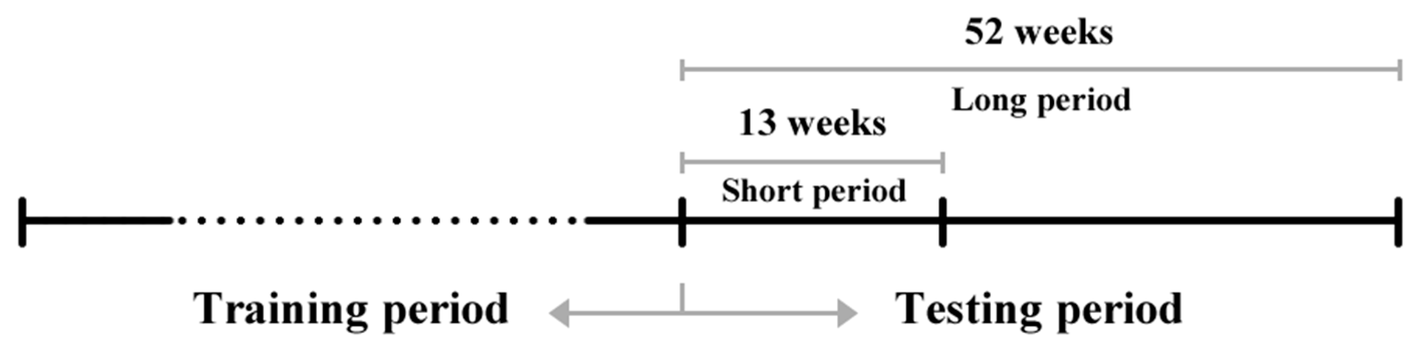
After the pre-processing and data exploration, the following procedure was established for the comparison of the individual models. First, the training and testing periods to carry out the prediction were defined. Two testing periods were selected for the prediction: long (52 weeks) and short (13 weeks), see Figure 2. In order to make the most of the available data, the last 52 weeks from each dataset were separated, and the data were used for the evaluation of the models’ prediction performance in both long and short testing periods. The remaining data (the total number of weeks without the final 52 weeks) serves as the training period, and its lengths differ per each data set.
Data in the testing period were then cleansed of newcomer customers, as the prediction was compared with reality only for the customers who were acquired before the testing period. Short- and long-term comparisons were made from two perspectives—at the individual and the aggregated customer base level in accordance with [12].
The customer base level offers an overall perspective and compares the real situation with the prediction of CLV for all the customers together. The performance of the models for the whole short and long periods (Forecast vs Actual metric) was evaluated, and the weekly model performance was also assessed using the mean absolute percentage error (MAPE).
The Forecast vs Actual metric is defined as
where At is the sum of actual profits over all customers in time t, Ft is the sum of forecast profits over all customers in time t; p is the threshold of the prediction and h is its horizon.
MAPE also compares the forecasts with actual values and uses the formula
where (h − p + 1) is the length of the testing period.
Another perspective compares the prediction at individual customer level. The original intention was to construct the MAPE metric as well; however, this metric would use the actual value of profit in the denominator, which is often equal to zero (for customers who did not make any purchase during the testing period).
Therefore, the mean absolute error (MAE) was used instead, which is defined as
where Ai is the sum of actual profits from the i-th customer over the whole testing period, Ft is the sum of forecasted profits from the i-th customer over the entire testing period, and n is the number of customers.
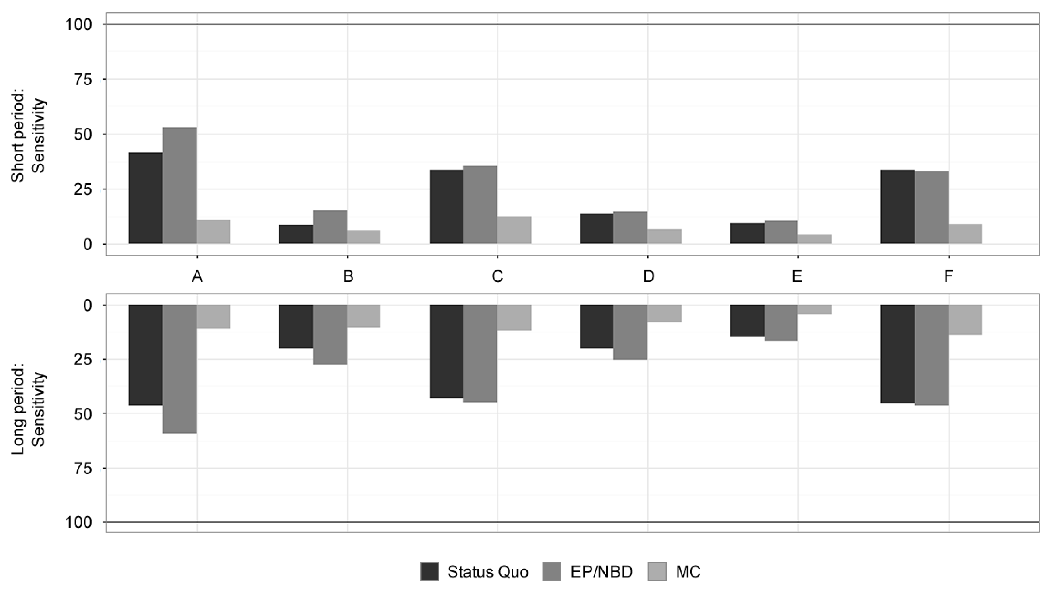
Although MAE in the percentage of the average actual profit would be preferable, it seemed reasonable to use the same metric as [12] for the sake of comparison: MAE in the percentage of average CLV. The reason for this decision is the possibility of broader theorizing about the results of various studies in case the researchers used the same statistical or evaluation metrics. The success rate of selecting the most profitable customers was also evaluated. Using the individual models, 10% of the most profitable customers were selected in the short and the long period and compared with the actual top 10%. To compare the performance of this classification, sensitivity (sometimes called true positive rate or recall) is computed as
where TP (true positives) is the number of customers assigned correctly to the top 10% class, and FN (false negatives) is the number of customers that were not assigned to the top 10% by the CLV calculation but which actually belonged to this class.
4. Results
This article aims to empirically compare the predictive ability and quality of selected CLV models on the basis of statistical metrics. This part presents the results of each model for every dataset by the selected performance metrics of Forecast vs Actual, MAE on a customer level, MAPE on a weekly basis, and sensitivity for identifying 10% of the most profitable customers. All the results are compared both for a short-term prediction period of 13 weeks and a long-term prediction of 52 weeks of calculated CLV. Evaluation metrics overview and comparison methodology are presented in Section 3.4. Further discussion and implications of the results are presented in Section 5. A visual comparison of results can be found in Appendix A (Figure A1, Figure A2, Figure A3 and Figure A4).
For results interpretation, it is important to emphasize that a quality of some results corresponds to the complex prediction subject: the models not only aim at estimating purchase probability, purchase frequency and purchase value, but the final variable is the profit in time.
It can be stated that undervaluation of the customer base offers better insights and possible applications than overestimation. As the results in Table 3 indicate, the best model for predicting customer base value for the short term period is the Status Quo model, reaching an average 91% of the actual profits. However, it appears extremely inconsistent in predictions as judged by the standard deviation and high overvaluation of the profit value for the majority of datasets except the dataset F. The EP/NBD model shows a solid performance with 62% of actual profit and good standard deviation. The worst model by short-term predictive performance is the MC model with a strong undervaluation of 54% of actual profit and the highest standard deviation from the researched models.
For the long-term period, results in Table 3 reveal that the best model for predicting customer base value is the EP/NBD model with 93% of actual profit. Very stable results regarding standard deviation are negatively impacted only by the fact that it overestimates the value for all datasets except for online store F. The MC model has excellent performance, reaching 82% of actual profit, but the inconsistency as seen by standard deviation and the comparison with short-term results leave quite poor conclusions for this model. The worst model in the long-term results is the Status Quo model, due to its overestimation of customer base value reaching 138% of actual profit on average.
Weekly predictions for the short-term period shown in Table 4 are well covered by EP/NBD models, reaching MAPE of 43%, respectively, with very low standard deviation. Status Quo and MC models performed poorly with high standard deviation and MAPE of 59% and 63%, respectively.
In the long-term period, the EP/NBD model performed very well with MAPE of 21%, respectively, as shown in Table 4. MAPE results were better in the long-term period and understandably worse standard deviation than in short-term with this model. The MC and Status Quo models achieved bad results similar to their short-term performance with MAPE of 50% and 64%, respectively, and also with high variance of results.
Table 5 summarises the results for mean absolute error (MAE). The lowest errors in the short-term period can be observed for the Status Quo model (MAE of 147% on average) with results almost comparable to the EP/NBD model (MAE of 191% on average). The MC model performs poorly (MAE of 294%) mainly because of its bad performance on dataset F. All models have a relatively low standard deviation, which can be seen as a good indicator of their quality.
For the long-term period, both Status Quo and EP/NBD models perform very well with MAE of 93% and 114%, respectively, as shown in Table 5. Worse results were displayed by the EP/NBD model for dataset E with MAE of 165%. Both of these models performed very well working on the largest dataset F with the Status Quo model reaching MAE of 92% and the EP/NBD model achieving MAE of 112%. The MC model does not perform that well (MAE of 190% on average, with the best result of 104% for dataset B). All models deliver consistent results as seen by the low standard deviations.
Table 6 summarises the results for the sensitivity of selecting 10% of the most profitable customers. Short-term period results indicate that the MC model with a sensitivity of 8.95% has not beaten even the random selection baseline of 10%. The best models for selecting the most valuable customers in the short-term period are EP/NBD and Status Quo models, with a sensitivity of 32% and 31%, respectively.
Long-term period results of sensitivity reveal EP/NBD and Status Quo as the two best models for the selection of highly valuable customers, achieving a sensitivity of 43% and 41%, respectively, and having reasonable standard deviations of 22% and 18%, respectively, see Table 6 for more details. For datasets A, C and F, robust and similar performance was achieved by both of these models, with the EP/NBD model having a slight improvement of sensitivity for dataset C (shift from 43% to 45%) and dataset F (shift from 45% to 46%) and strong improvement of sensitivity for dataset A (shift from 47% to 59%). The MC model still performs poorly, resulting in the sensitivity of 13% with no exceptional results for any dataset. All the models show better sensitivity results in comparison with the short-term period.
A conclusion can be drawn from all these results to answer the research question from Section 1: Which of the compared models for calculating CLV have a good predictive performance of CLV in the non-contractual environment of e-commerce? The results described in this section demonstrate that the EP/NBD model has consistently outperformed other selected models in a majority of evaluation metrics and can be thus considered good and stable for online shopping within e-commerce business. Its predictive power was recognised both in short- and long-term periods and also when comparing individual predictions with overall customer base value prediction.
5. Discussion and Implications
Section 2 introduced the main conclusions of the articles [12,13]. Like this article, they base their conclusions on their empirical comparison of selected models. In contrast, there exists a significant number of reviews comparing theoretical aspects of selected CLV models based on results from secondary sources that build on different datasets and focus on various types of environment and applications. This article compares models representing different approaches to modeling CLV and also compares other models than those selected for comparison with the articles above [12,13]—both studies deal with different environments and use a single dataset for the evaluation of selected models.
The results in Section 4 offer new insights into the performance of two complex models and a very simple one, considering six different datasets typical for online shopping. All selected models use the same minimal dataset and also the same data concerning recency and frequency of orders. The MC model then uses additional data required as input parameters. All models selected for the comparative analysis also have in common the fact that despite different calculation methods and input parameters, they all have the same output, or purpose: calculating customer lifetime value. That makes this a relevant comparative analysis of CLV calculation results. Here follows a discussion of the results of each model and possible explanations of its performance.
The EP/NBD model performed consistently well both in individual predictions and overall customer base. Slightly bad results for datasets D and E according to MAE for long-term period correlate with lower repurchase frequency of these retailers’ customers. This observation is backed by the feature of the spending submodel used in the EP/NBD model. Whenever a customer features a low number of total transactions (might as well be a new customer with a single order), the Gamma-Gamma spending submodel predicts their lifetime average order value considering predominantly the rest of the customer population. With more orders completed, increasingly more weight is attributed to customer’s purchase behavior, and the rest of the population plays a minor role. Therefore, if a dataset contains only a few customers with repeated purchases, the spending model will prefer more population estimates and the EP/NBD model results will be driven mainly by the Pareto/NBD submodel (Recency and Frequency).
The Status Quo model overestimates customer base profit value for the majority of datasets, except for C and F, as seen in Table 3. Recency and frequency analysis of the training period reveal that both datasets C and F consist of a very high ratio of customers with low profitability and low purchase frequency with two completed transactions at most. This customer cluster does not impact the results of the rest of the datasets to such an extent. Also observed was an undervaluation of customer-level profit prediction for segments of customers with interpurchase times higher than the threshold of 52 weeks chosen for the Status Quo model. This effect was mainly observed for datasets A, B and E, which include approximately 30% of the customers with second-transaction repurchase interval longer than 52 weeks. Customer segments with high purchase frequency result in overestimation of profit prediction by neglecting dropout signals.
These results indicate that the Status Quo model could be beneficial in situations with low or predictable dropout rates, with a stronger likelihood of higher purchase frequency and low variability in product margin—compare with [12]. The methodology for the Status Quo model is the simplest and most understandable, yet confusing regarding the description of the underlying customer behavior. However, in comparison with other models used in this research, it must be concluded that the features of the Status Quo model are not suitable for datasets with long training time periods and large data sets with high customer heterogeneity including spontaneous purchase behavior undergoing significant changes in time.
The results of the MC model appear to be very erratic across all the datasets and evaluation metrics. There was a high standard deviation for customer base level prediction (see Table 3) and weekly trends (see Table 4). From this analysis of the MC model results, it can be concluded that the performance relies heavily on the quality of the initial subgroups found in the first part of the model execution. These subgroups are estimated by a decision tree, which could benefit from as much customer level data as possible. According to the methodology described in Section 3.2, it was possible to use only attributes (profitability drivers) available for all datasets. The quality of subgroups corresponds with the weakly results and performance of the Markov chain submodel and implies the need for such customer attributes. It could be recommended to determine more profitability drivers and maintain a thorough analysis of input variables for this model. A remarkable exception to this conclusion is found in the dataset E that initially identified clear subgroups in the CART submodel, yet the results of classification of the most profitable customers in Table 6 demonstrate weak performance with a sensitivity of only 4%, while random selection would roughly result in 10% sensitivity. The underperformance of MC customer classification compared to random selection was unanticipated.
It can be summarised that the EP/NBD model performed very well on all selected datasets, achieved stable results both on customer level and for the whole customer base metrics. The Status Quo model demonstrated strong results in the selection of the top 10% of the most profitable customers and had low individual customer level error rates, which could be seen as a good result for this naïve model construction. The results were negatively influenced mainly by the large overvaluation of the customer base for the majority of datasets in both the short- and long-term period the MC model performed with the worst results on all levels: achieving poor performance on an individual customer level, in the selection of the top 10% of the most profitable customers, and even when considering the overall customer base value.
Seasonality (e.g., the Christmas period) constitutes a problem for all datasets containing predominantly seasonal purchase behavior. That has a strong impact mainly for datasets B and D with the EP/NBD model, and this impact can be associated with the fact that the training period ended in late November, i.e., in the midst of the Christmas season for online stores. On the other hand, as all datasets included at least three years of data (dataset B missing just one month), this can be seen as equal input conditions for model training and the following comparison.
5.1. Managerial Implications
Our findings suggest that outputs from CLV models can be used at several levels of detail with very satisfying error rates. Managers need to decide on the level of detail required for the specific application. Three main possibilities include individual customer level, segmented groups of customers and overall customer base level predictions:
- Individual customer level has a wide range of applications from marketing campaign selection to customer support preferences. Individual customer scoring, as expressed by the selection of the top 10% of the most profitable customers, needs to be addressed with business goals in mind. For practical utilization, this means considering whether to include or exclude such customers from marketing campaigns. Experimentation with a segmented or even personalised campaign in order to leverage and support the expected high value from such customers is advised. For classification into top 10% of the most profitable customers the sensitivity is an important metric in order to assess the model’s ability to execute the correct classification of top customers, which could be useful for the selection of specific marketing campaigns.
- Segmented groups of customers are well suited for aggregated analysis of customer base growth drivers.
- Customer base level of CLV applications is useful in business planning and strategic management.
As the metrics evaluated in Section 4 resulted in specific advantages of each of the CLV models, managers need to assess the main outputs of CLV models with additional benefits and disadvantages that the model offers. For the most basic use, the Status Quo model brings agreeable results despite its simplicity and naïve approach. Its results are suitable for online stores with customer homogeneity and low variance in product margins. The EP/NBD model showed very good results highly suitable for studied e-commerce business settings, outputting not only CLV but also the probability of a customer being live in the following period. The MC model performed poorly, and it would be recommended to focus more on the input data and initial customer clustering, which has a significant impact on these results. For a successful implementation and performance of CLV models, it is necessary for the company to maintain profit data on individual transaction level. This constraint impacts not only the accounting processes but also requires the product and marketing cost data to be included in profit calculations. The presented empirical analysis shows that using only basic transaction data in the EP/NBD model provides satisfying and stable quality predictions in various application contexts in online shopping. Incorporating multiple types of customer data into the models that allow or need it does not guarantee improvements in predictive performance (see the results of MC model). For these models, a validation of data enrichment incremental impact on the predictive model is essential to achieve results more relevant to determined business goals. The reason for proposing such an intensive preparation is that it captures the relations between internal and external data in the specific business context. The EP/NBD model has outperformed other selected models in a majority of evaluation metrics and can be considered good enough for non-contractual relations in online shopping within e-commerce business.
5.2. Limitations and Further Research Directions
Due to the selected experiment method, restrictions on minimal data length were identified. As discussed in Section 3.4, for individual customer level error metric MAE (in %) as [12] was followed, i.e., the average predicted profit value as a base for comparison. The authors suggest a thorough comparison with alternative calculation using actual profit values in the denominator. Moreover, the evaluation of models could be more detailed and insightful with an analysis of the distribution of differences between predicted and actual profit values in the testing period.
Problems have been experienced with the low speed of the EP/NBD model fitting due to the long run of the optimization function for the estimation of main parameters (r, α, s, β) for the transaction frequency submodel. No simple relationship was observed between the time required for parameter fitting and the number of customers in the dataset. As the speed of the EP/NBD model caused several issues, three directions for optimization would be recommended:
- A thorough analysis of the time constraints in model execution.
- Using optimization method for likelihood minimization of parameter estimation that does not allow box constraints.
- Rewriting model execution to support parallel computing, at least for the parameter estimation.
All of the selected models performed poorly for seasonal purchase behavior, mainly during and after the Christmas season. Such seasonal effects were not discussed in the empirical studies by [12,13]. A model that either considered monthly cohorts or incorporated seasonal effects of time series could perform better. The decision tree in MC could make use of a variable indicating either acquisition date or purchase date. It could then be expected that such improvement benefits mostly the online stores with strong Christmas season and also companies eager to estimate not only the sum of lifetime value but the trended data of such predictions as well. No other strong relations with other season holidays throughout the year were identified.
Recency and frequency analysis of the datasets suggest that there are customers with frequent purchase behavior. The predictive power could be better for these. The topic of purchase regularity and interpurchase timing was researched by [66] and their results indicate that regularity highly improves predictability. On the other hand, high regularity can go against the specified attributes of business settings (see Section 3.1).
An opportunity could be seen in a combination of several models that would better capture the underlying customer behavior. As discussed in Section 3.1, the EP/NBD model is an example of such a model being composed of two submodels. Platzer and Reutterer [66] introduce a new model labelled Pareto/GGG, which incorporates interpurchase timing as a regularity submodel to take into consideration customers with a clear pattern of purchase behavior and to deal reasonably with those showing purchase irregularities. McCarthy et al. [67] estimate variance of CLV. Clearly, the next phase for model combinations could be the use of ensemble learning.
The presented research provides several insights, using an empirical analysis of real online store datasets and a comparison of selected models for CLV computation. More empirical studies would be welcomed: ones that would study datasets from outside the Eastern European area, in order to see if the same results could be found globally, and studies that would focus on a comparison of recently researched models from both performance and feature perspectives, resulting in a development of more robust yet customizable general CLV models. The EP/NBD model has very good results in this study, so it would be appropriate to perform similar empirical comparisons for various modifications of this model, mentioned e.g., in [13,50,58,65,68].
Acknowledgments
This research was prepared thanks to the grant (F4/18/2014) of the University of Economics, Prague.
Author Contributions
Pavel Jasek defined methodology, formulated the research question, obtained datasets from selected online stores and prepared models implementation. Lenka Vrana prepared statistical analysis and models implementation. Lucie Sperkova pre-processed the data and analyzed the results. Zdenek Smutny prepared a literature review and defined methodology. Marek Kobulsky prepared models implementation. All authors participated in the evaluation of the results. The manuscript was written equally together.
Conflicts of Interest
The authors declare no conflict of interest.
Appendix A
Figure A1.
Results for Forecast vs. Actual (in %) for online stores A–F. Source: Authors.
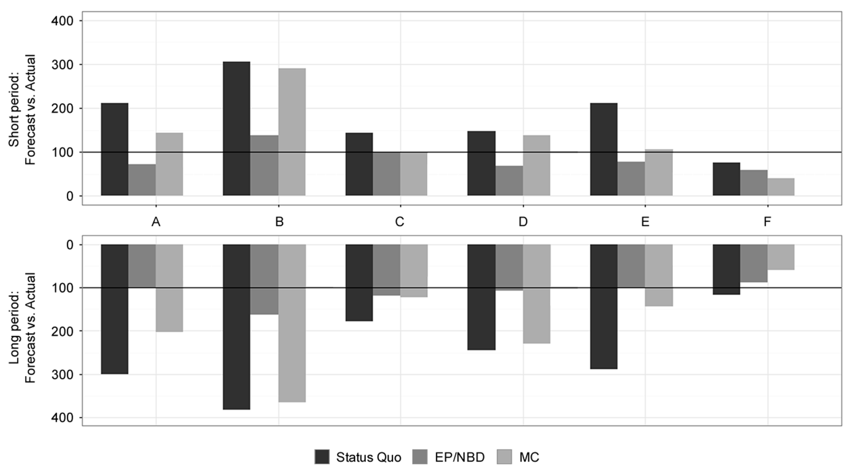
Figure A2.
Results for MAPE (weekly-level, in %) for online stores A-F. Source: Authors.
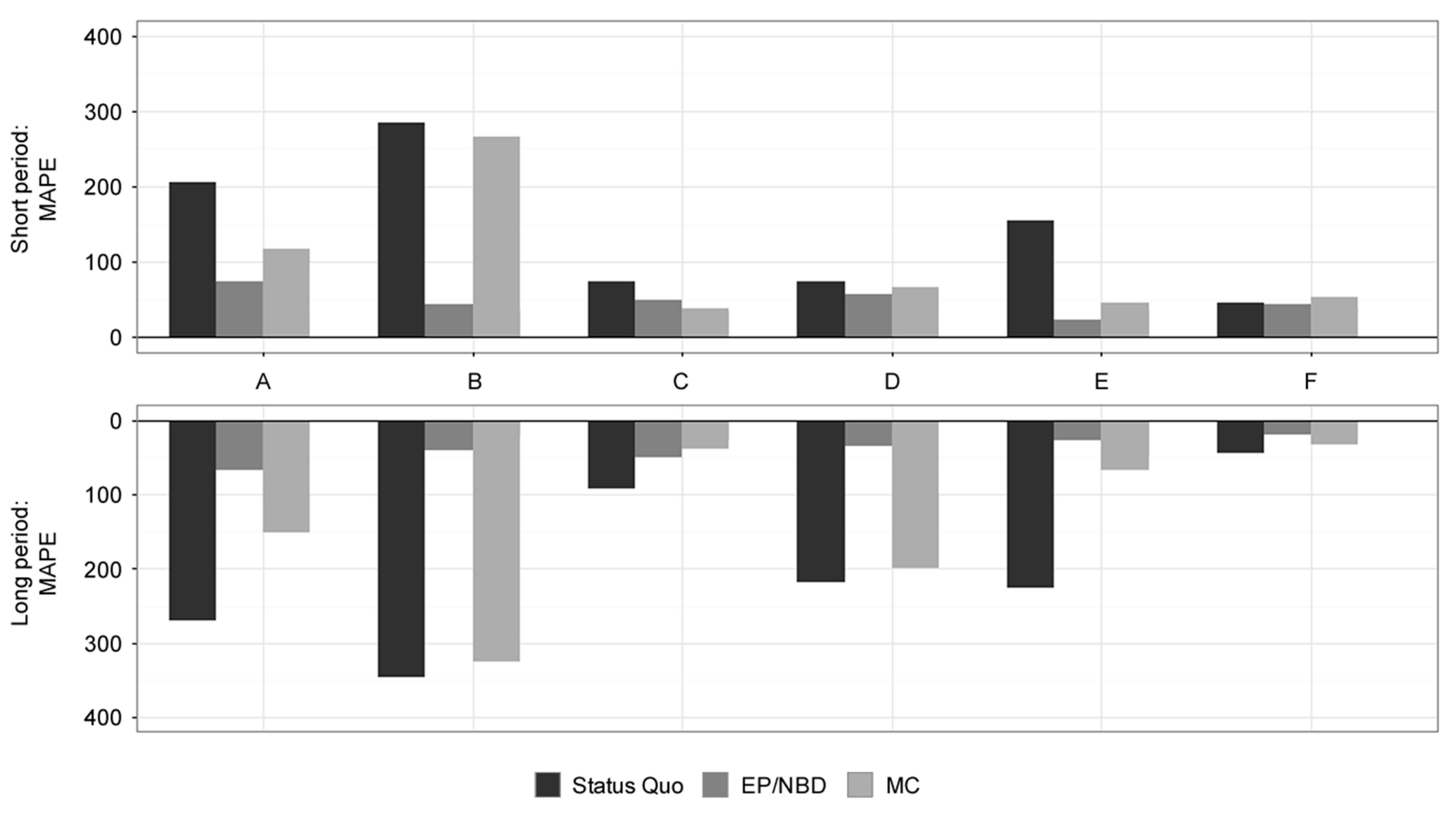
Figure A3.
Results for MAE (customer-level, in %) for online stores A-F. Source: Authors.
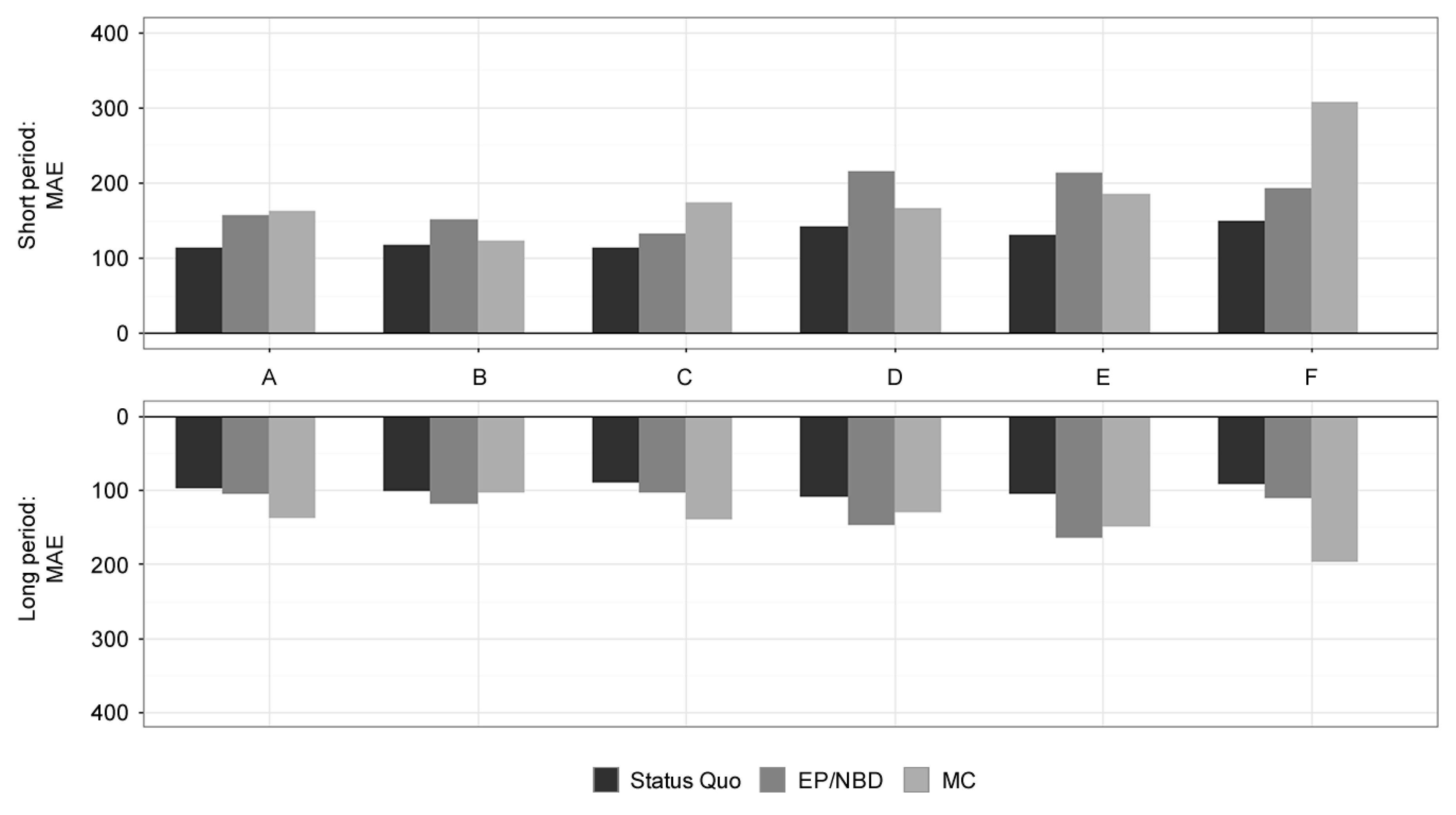
Figure A4.
Results for Sensitivity (customer-level, in %) for online stores A-F. Source: Authors.
References
- Haenlein, M.; Kaplan, A.M.; Schoder, D. Valuing the Real Option of Abandoning Unprofitable Customers When Calculating Customer Lifetime Value. J. Mark. 2006, 70, 5–20. [Google Scholar] [CrossRef]
- Online Retailing: Britain, Europe, US and Canada 2015. Centre for Retail Research. Available online: http://www.retailresearch.org/onlineretailing.php (accessed on 27 December 2017).
- Jain, D.C.; Singh, S.S. Customer lifetime value research in marketing: A review and future directions. J. Interact. Mark. 2002, 16, 34–46. [Google Scholar] [CrossRef]
- Fader, P.S.; Hardie, B.G.S. Probability Models for Customer-Base Analysis. J. Interact. Mark. 2009, 23, 61–69. [Google Scholar] [CrossRef]
- Damm, R.; Monroy, C.R. A review of the customer lifetime value as a customer profitability measure in the context of customer relationship management. Intang. Cap. 2011, 7, 261–279. [Google Scholar] [CrossRef]
- Chang, W.; Chang, C.; Li, Q. Customer Lifetime Value: A Review. Soc. Behav. Personal. 2012, 40, 1057–1064. [Google Scholar] [CrossRef]
- Estrella-Ramón, A.M.; Sánchez-Pérez, M.; Swinnen, G.; VanHoof, K. A marketing view of the customer value: Customer lifetime value and customer equity. S. Afr. J. Bus. Manag. 2013, 44, 47–64. [Google Scholar]
- EsmaeiliGookeh, M.; Tarokh, M.J. Customer Lifetime Value Models: A literature Survey. Int. J. Ind. Eng. Prod. Res. 2013, 24, 317–336. [Google Scholar]
- Singh, S.S.; Jain, D.C. Measuring Customer Lifetime Value: Models and Analysis. INSEAD Working Paper No. 2013/27/MKT 2013. [Google Scholar] [CrossRef]
- Rozek, J.; Karlicek, M. Customer Lifetime Value as the 21st Century Marketing Strategy Approach. Cent. Eur. Bus. Rev. 2014, 3, 28–35. [Google Scholar] [CrossRef]
- Gupta, S.; Hanssens, D.; Hardie, B.; Kahn, W.; Kumar, V.; Lin, N.; Ravishanker, N.; Sriram, S. Modeling Customer Lifetime Value. J. Serv. Res. 2006, 9, 139–155. [Google Scholar] [CrossRef]
- Donkers, B.; Verhoef, P.C.; De Jong, M.G. Modeling CLV: A test of competing models in the insurance industry. Quant. Mark. Econ. 2007, 5, 163–190. [Google Scholar] [CrossRef]
- Batislam, E.M.; Denizel, M.; Filiztekin, A. Empirical Validation and Comparison of Models for Customer Base Analysis. Int. J. Res. Mark. 2007, 24, 201–209. [Google Scholar] [CrossRef]
- Dresch, A.; Lacerda, D.P.; Antunes, J.A.V., Jr. Design Science Research: A Method for Science and Technology Advancement; Springer: Berlin, Germany, 2015. [Google Scholar]
- Hubka, V.; Eder, W.E. Design Science: Introduction to the Needs, Scope and Organization of Engineering Design Knowledge; Springer: Berlin, Germany, 1996. [Google Scholar]
- Wieringa, R.J. Design Science Methodology for Information Systems and Software Engineering; Springer: Berlin, Germany, 2014. [Google Scholar]
- Kumar, V.; Pansari, A. National Culture, Economy, and Customer Lifetime Value: Assessing the Relative Impact of the Drivers of Customer Lifetime Value for a Global Retailer. J. Int. Mark. 2016, 24, 1–21. [Google Scholar] [CrossRef]
- Persson, A. Profitable Customer Management: A Study in Retail Banking; Hanken School of Economics: Helsinki, Finland, 2011. [Google Scholar]
- Hevner, A.R.; Chatterjee, S. Design Research in Information Systems: Theory and Practice; Springer: London, UK, 2010. [Google Scholar]
- Kotler, P.; Keller, K.L. Marketing Management, 15th ed.; Prentice Hall: Upper Saddle River, NJ, USA, 2015. [Google Scholar]
- Kumar, V.; Pozza, I.D.; Petersen, J.A.; Denish Shah, D. Reversing the Logic: The Path to Profitability through Relationship Marketing. J. Int. Mark. 2009, 23, 147–156. [Google Scholar] [CrossRef]
- Fader, P.S. Customer Centricity: Focus on the Right Customers for Strategic Advantage; Wharton Digital Press: Philadelphia, PA, USA, 2012. [Google Scholar]
- Doyle, P. Value-based marketing. J. Strateg. Mark. 2000, 8, 299–311. [Google Scholar] [CrossRef]
- Srivastava, R.K.; Shervani, T.A.; Fahey, L. Market-Based Assets and Shareholder Value: A Framework for Analysis. J. Mark. 1998, 62, 2–18. [Google Scholar] [CrossRef]
- Gupta, S. Customer-Based Valuation. J. Interact. Mark. 2009, 23, 169–178. [Google Scholar] [CrossRef]
- Persson, A.; Ryals, L. Customer assets and customer equity: Management and measurement issues. Mark. Theory 2010, 10, 417–436. [Google Scholar] [CrossRef]
- Ryals, L.; Knox, S. Measuring and managing customer relationship risk in business markets. Ind. Mark. Manag. 2007, 36, 823–833. [Google Scholar] [CrossRef] [Green Version]
- Kim, S.-Y.; Jung, T.-S.; Suh, E.-H.; Hwang, H.-S. Customer segmentation and strategy development based on customer lifetime value: A case study. Expert Syst. Appl. 2006, 31, 101–107. [Google Scholar] [CrossRef]
- Hwang, H.; Jung, T.; Suh, E. An LTV model and customer segmentation based on customer value: A case study on the wireless telecommunication industry. Expert Syst. Appl. 2004, 26, 181–188. [Google Scholar] [CrossRef]
- Singh, S.S.; Jain, D.C. Measuring Customer Lifetime Value. In Review of Marketing Research; Naresh, K.M., Ed.; Emerald Group Publishing Limited: Bingley, UK, 2010; Volume 6, pp. 37–62. [Google Scholar]
- Pfeifer, P.E.; Haskins, M.E.; Conroy, R.M. Customer Life Time Value, Customer Profitability, and the Treatment of Acquisition Spending. J. Manag. Issues 2005, 17, 11–25. [Google Scholar]
- Boyce, G. Valuing customers and loyalty: The rhetoric of customer focus versus the reality of alienation and exclusion of (de valued) customers. Crit. Perspect. Account. 2000, 11, 649–689. [Google Scholar] [CrossRef]
- Ryals, L. Profitable relationships with key customers: How suppliers manage pricing and customer risk. J. Strateg. Mark. 2006, 14, 101–113. [Google Scholar] [CrossRef] [Green Version]
- Ryals, L. Are your customers worth more than money? J. Retail. Consum. Serv. 2002, 9, 241–251. [Google Scholar] [CrossRef]
- Williams, C.; Williams, R. Optimizing acquisition and retention spending to maximize market share. J. Mark. Anal. 2015, 3, 159–170. [Google Scholar] [CrossRef]
- Abdolvand, N.; Baradaran, V.; Albadvi, A. Activity-level as a link between customer retention and consumer lifetime value. Iran. J. Manag. Stud. 2015, 8, 567–587. [Google Scholar]
- Qi, J.Y.; Qu, Q.X.; Zhou, Y.P.; Li, L. The impact of users’ characteristics on customer lifetime value raising: Evidence from mobile data service in China. Inf. Technol. Manag. 2015, 16, 273–290. [Google Scholar] [CrossRef]
- Nenonen, S. Storbacka, K. Driving shareholder value with customer asset management: Moving beyond customer lifetime value. Ind. Mark. Manag. 2016, 52, 140–150. [Google Scholar] [CrossRef]
- Blattberg, R.C.; Getz, G.; Thomas, J.S. Customer Equity: Building and Managing Relationships as Valuable Assets; Harvard Business Press: Boston, MA, USA, 2001. [Google Scholar]
- Rust, R.T.; Lemon, K.N.; Zeithaml, V.A. Return on Marketing: Using Customer Equity to Focus Marketing Strategy. J. Mark. 2004, 68, 109–127. [Google Scholar] [CrossRef]
- Gupta, S.; Lehmann, D.R.; Stuart, J.A. Valuing Customers. J. Mark. Res. 2004, 41, 7–18. [Google Scholar] [CrossRef]
- Zhang, J.Q.; Dixit, A.; Friedmannc, R. Customer Loyalty and Lifetime Value: An Empirical Investigation of Consumer Packaged Goods. J. Mark. Theory Pract. 2010, 18, 127–140. [Google Scholar] [CrossRef]
- Blattberg, R.C.; Deighton, J. Manage Marketing by the Customer Equity Test. Harv. Bus. Rev. 1996, 74, 136–144. [Google Scholar] [PubMed]
- Berger, P.D.; Nasr, N.I. Customer Lifetime Value: Marketing Models and Applications. J. Interact. Mark. 1998, 12, 17–30. [Google Scholar] [CrossRef]
- European B2C E-commerce Report 2016; Ecommerce Foundation: Brussels, Belgium, 2017.
- E-commerce in Europe 2015. Available online: http://www.postnord.com/globalassets/global/english/document/publications/2015/en_e-commerce_in_europe_20150902.pdf (accessed on 27 December 2017).
- Fader, P.S.; Hardie, B.G.S.; Lee, K.L. Counting your Customers the Easy Way: An Alternative to the Pareto/NBD Model. Mark. Sci. 2005, 24, 275–284. [Google Scholar] [CrossRef]
- Haenlein, M.; Kaplan, A.M.; Beeser, A.J. A Model to Determine Customer Lifetime Value in a Retail Banking Context. Eur. Manag. J. 2007, 25, 221–234. [Google Scholar] [CrossRef]
- Paauwe, P.; Van der Putten, P.; Van Wezel, M. DTMC: An actionable e-customer lifetime value model based on markov chains and decision trees. In Proceedings of the Ninth International Conference on Electronic Commerce (ICEC ‘07), Minneapolis, MN, USA, 19–22 August 2007; pp. 253–262. [Google Scholar]
- Villanueva, J.; Yoo, S.; Hanssens, D.M. The Impact of Marketing-Induced Versus Word-of-Mouth Customer Acquisition on Customer Equity Growth. J. Mark. Res. 2008, 45, 48–59. [Google Scholar] [CrossRef]
- Jerath, K.; Fader, P.S.; Hardie, B.G.S. New Perspectives on Customer “Death” Using a Generalization of the Pareto/NBD Model. Mark. Sci. 2011, 30, 866–880. [Google Scholar] [CrossRef]
- Schmittlein, D.C.; Morrison, D.G. Prediction of Future Random Events with the Condensed Negative Binomial Distribution. J. Am. Stat. Assoc. 1983, 78, 449–456. [Google Scholar] [CrossRef]
- Schmittlein, D.C.; Bemmaor, A.C.; Morrison, D.G. Technical Note—Why Does the NBD Model Work? Robustness in Representing Product Purchases, Brand Purchases and Imperfectly Recorded Purchases. Mark. Sci. 1985, 4, 255–266. [Google Scholar] [CrossRef]
- Schmittlein, D.C.; Morrison, D.G.; Colombo, R. Counting Your Customers—Who Are They and What Will They Do Next. Manag. Sci. 1987, 33, 1–24. [Google Scholar] [CrossRef]
- Colombo, R.; Jiang, W. A Stochastic RFM Model. J. Interac. Mark. 1999, 13, 2–12. [Google Scholar] [CrossRef]
- Fader, P.S.; Hardie, B.G.S. Forecasting Repeat Sales at CDNOW: A Case Study. Interfaces 2001, 31, S94–S107. [Google Scholar] [CrossRef]
- Adomavicius, G.; Tuzhilin, A. Toward the next generation of recommender systems: A survey of the state-of-the-art and possible extensions. IEEE Trans. Knowl. Data Eng. 2005, 17, 734–749. [Google Scholar] [CrossRef]
- Knox, G.; van Oest, R. Customer Complaints and Recovery Effectiveness: A Customer Base Approach. J. Mark. 2014, 78, 42–57. [Google Scholar] [CrossRef]
- Gladya, N.; Baesensa, B.; Crouxa, C. A modified Pareto/NBD approach for predicting customer lifetime value. Expert Syst. Appl. 2009, 36, 2062–2071. [Google Scholar] [CrossRef]
- Schmittlein, D.C.; Peterson, R.A. Customer Base Analysis: An Industrial Purchase Process Application. Mark. Sci. 1994, 13, 41–67. [Google Scholar] [CrossRef]
- Reinartz, W.J.; Kumar, V. On the Profitability of Long-Life Customers in a Noncontractual Setting: An Empirical Investigation and Implications for Marketing. J. Mark. 2000, 64, 17–35. [Google Scholar] [CrossRef]
- Fader, P.S.; Hardie, B.G.S.; Lee, K.L. RFM and CLV: Using Iso-Value Curves for Customer Base Analysis. J. Mark. Res. 2005, 42, 415–430. [Google Scholar] [CrossRef]
- Fader, P.S.; Hardie, B.G.S. The Gamma-Gamma Model of Monetary Value, 2013. Available online: http://www.brucehardie.com/notes/025/gamma_gamma.pdf (accessed on 27 December 2017).
- Pfeifer, P.E.; Carraway, R.L. Modeling customer relationships as Markov chains. J. Interact. Mark. 2000, 14, 43–55. [Google Scholar] [CrossRef]
- Burcher, N. Paid, Owned, Earned: Maximising Marketing Returns in a Socially Connected World; Kogan Page: Philadelphia, PA, USA, 2012. [Google Scholar]
- Platzer, M.; Reutterer, T. Ticking Away the Moments: Timing Regularity Helps to Better Predict Customer Activity. Mark. Sci. 2016, 35, 779–799. [Google Scholar] [CrossRef]
- McCarthy, D.; Fader, P.S.; Hardie, B.G.S. V(CLV): Examining Variance in Models of Customer Lifetime Value. Available online: https://papers.ssrn.com/sol3/papers.cfm?abstract_id=2739475 (accessed on 27 December 2017).
- Casterán, H.; Meyer-Waarden, L.; Reinartz, W. Modeling Customer Lifetime Value, Retention, and Churn. In Handbook of Market Research; Homburg, C., Klarmann, M., Vomberg, A., Eds.; Springer: Berlin, Germany, 2017; pp. 1–33. [Google Scholar]
Figure 1.
Methodology of the research with six phases. Source: Authors.

Figure 2.
Data division for comparison. Source: Authors.

Table 1.
Five randomly selected rows from the complete dataset, consisting of the minimal dataset and data added especially for the MC model.
Table 1.
Five randomly selected rows from the complete dataset, consisting of the minimal dataset and data added especially for the MC model.
| Dataset (Online Store) | Common Data Used by All Four Models (Minimal Dataset) | Specially Added Data for MC Model | ||||||||||
|---|---|---|---|---|---|---|---|---|---|---|---|---|
| Customer_ID | Week_Number | Monday_Date | Profit_EUR | Channel_POE | Channel_Type | Medium_Source | Avg_Purchase_Day | Item_Quantity | Transaction_Shippin | Transaction_Revenue | Zip_firstchar | |
| B | 282006 | 98 | 2014-11-17 | 7.69 | O | email_newsletter | 3.0 | 1 | 1.19 | 23.90 | 1 | |
| D | 65298 | 302 | 2014-09-15 | 11.84 | E | organic | organic_google | 4.5 | 1 | 0.00 | 42.96 | 8 |
| F | 1182543 | 158 | 2013-01-07 | 7.37 | P | email_newsletter | 4.0 | 4 | 0.00 | 33.52 | 3 | |
| F | 883193 | 103 | 2011-12-19 | 3.48 | P | campaign | cpc_google | 4.0 | 1 | 0.00 | 37.74 | 5 |
| F | 1349757 | 197 | 2013-10-07 | 6.96 | P | feed | feed_heureka | 2.0 | 3 | 0.00 | 62.00 | 6 |
Source: Authors.
Table 2.
Summary information about individual online stores and available data.
| Dataset (Online Store) | Number of Transactions | Number of Customers | Sum of Profit EUR | Average Transaction Profit EUR | Data Range (In Weeks) |
|---|---|---|---|---|---|
| A | 19,433 | 14,758 | 148,999 | 7.87 | 218 |
| B | 136,611 | 90,896 | 2,573,842 | 19.24 | 151 |
| C | 106,129 | 50,255 | 557,085 | 5.53 | 173 |
| D | 119,439 | 73,472 | 1,625,073 | 14.33 | 364 |
| E | 62,744 | 43,899 | 1,101,526 | 17.73 | 381 |
| F | 2,409,019 | 798,703 | 18,037,523 | 7.88 | 301 |
Source: Authors.
Table 3.
Results for Forecast vs Actual (in %).
| Forecast vs. Actual (in %) | Short Period (13 Weeks) | Long Period (52 Weeks) | ||||
|---|---|---|---|---|---|---|
| Dataset (Online Store) | Status Quo | EP/NBD | MC | Status Quo | EP/NBD | MC |
| A | 211.61 | 71.68 | 143.47 | 301.58 | 101.50 | 203.57 |
| B | 305.11 | 137.27 | 290.91 | 382.93 | 163.50 | 365.03 |
| C | 143.54 | 100.72 | 99.50 | 177.68 | 118.10 | 122.95 |
| D | 146.55 | 68.91 | 137.17 | 245.18 | 107.85 | 229.85 |
| E | 212.12 | 78.12 | 106.46 | 288.30 | 100.98 | 144.62 |
| F | 76.54 | 58.06 | 39.07 | 116.83 | 87.82 | 59.69 |
| Weighted mean (by profit) | 91.13 | 62.47 | 53.90 | 138.28 | 92.97 | 82.35 |
| Relative standard deviation (%) | 55.66 | 26.56 | 99.89 | 47.69 | 18.50 | 88.66 |
Source: Authors.
Table 4.
Results for MAPE (weekly level, in %).
| MAPE (Weekly Level, in %) | Short Period (13 Weeks) | Long Period (52 Weeks) | ||||
|---|---|---|---|---|---|---|
| Dataset (Online Store) | Status Quo | EP/NBD | MC | Status Quo | EP/NBD | MC |
| A | 206.36 | 74.48 | 116.65 | 269.73 | 66.48 | 151.74 |
| B | 284.09 | 43.97 | 266.14 | 346.08 | 40.44 | 325.23 |
| C | 73.17 | 49.22 | 38.01 | 92.94 | 49.14 | 38.04 |
| D | 74.14 | 57.38 | 67.04 | 217.40 | 34.48 | 198.87 |
| E | 155.06 | 23.68 | 44.75 | 226.14 | 26.41 | 67.88 |
| F | 45.09 | 43.32 | 53.19 | 43.78 | 18.88 | 33.36 |
| Weighted mean (by profit) | 58.61 | 43.41 | 62.89 | 64.36 | 20.50 | 50.43 |
| Relative standard deviation (%) | 87.67 | 8.36 | 69.88 | 117.79 | 30.06 | 137.69 |
Source: Authors.
Table 5.
Results for MAE (customer-level, in %).
| MAE (Customer Level, in %) | Short Period (13 Weeks) | Long Period (52 Weeks) | ||||
|---|---|---|---|---|---|---|
| Dataset (Online Store) | Status Quo | EP/NBD | MC | Status Quo | EP/NBD | MC |
| A | 113.15 | 156.17 | 162.47 | 97.20 | 105.24 | 138.29 |
| B | 116.87 | 151.28 | 123.02 | 101.42 | 118.03 | 103.58 |
| C | 113.27 | 132.94 | 174.49 | 90.25 | 102.55 | 138.94 |
| D | 140.84 | 214.65 | 165.58 | 108.72 | 146.70 | 130.54 |
| E | 130.20 | 213.40 | 185.69 | 105.93 | 164.67 | 148.81 |
| F | 148.58 | 191.80 | 308.01 | 91.86 | 111.62 | 197.56 |
| Weighted mean (by profit) | 146.50 | 190.51 | 294.18 | 93.04 | 113.70 | 189.74 |
| Relative standard deviation (%) | 5.05 | 5.35 | 15.52 | 3.72 | 7.32 | 11.74 |
Source: Authors.
Table 6.
Results for Sensitivity (customer level, in %).
| Sensitivity (Customer Level, in %) | Short Period (13 Weeks) | Long Period (52 Weeks) | ||||
|---|---|---|---|---|---|---|
| Dataset (Online Store) | Status Quo | EP/NBD | MC | Status Quo | EP/NBD | MC |
| A | 41.33 | 52.67 | 10.67 | 46.67 | 59.33 | 11.00 |
| B | 8.75 | 14.95 | 6.15 | 20.20 | 27.78 | 10.54 |
| C | 33.30 | 35.50 | 12.10 | 43.10 | 45.20 | 12.00 |
| D | 13.60 | 14.60 | 6.60 | 20.10 | 25.20 | 8.10 |
| E | 9.60 | 10.20 | 4.20 | 15.10 | 16.60 | 4.10 |
| F | 33.35 | 32.98 | 9.13 | 45.41 | 46.23 | 14.12 |
| Weighted mean (by customer base) | 31.30 | 31.55 | 8.95 | 41.64 | 43.36 | 13.21 |
| Relative standard deviation (%) | 21.85 | 19.26 | 13.32 | 21.88 | 17.88 | 16.21 |
Source: Authors.
© 2018 by the authors. Licensee MDPI, Basel, Switzerland. This article is an open access article distributed under the terms and conditions of the Creative Commons Attribution (CC BY) license (http://creativecommons.org/licenses/by/4.0/).
Share and Cite
MDPI and ACS Style
Jasek, P.; Vrana, L.; Sperkova, L.; Smutny, Z.; Kobulsky, M. Modeling and Application of Customer Lifetime Value in Online Retail. Informatics 2018, 5, 2. https://doi.org/10.3390/informatics5010002
AMA Style
Jasek P, Vrana L, Sperkova L, Smutny Z, Kobulsky M. Modeling and Application of Customer Lifetime Value in Online Retail. Informatics. 2018; 5(1):2. https://doi.org/10.3390/informatics5010002
Chicago/Turabian StyleJasek, Pavel, Lenka Vrana, Lucie Sperkova, Zdenek Smutny, and Marek Kobulsky. 2018. "Modeling and Application of Customer Lifetime Value in Online Retail" Informatics 5, no. 1: 2. https://doi.org/10.3390/informatics5010002
Note that from the first issue of 2016, this journal uses article numbers instead of page numbers. See further details here.