Exploiting Rating Abstention Intervals for Addressing Concept Drift in Social Network Recommender Systems


1
Department of Informatics and Telecommunications, University of Athens, 15784 Athens, Greece
2
Department of Informatics and Telecommunications, University of the Peloponnese, 22100 Tripolis, Greece
*
Author to whom correspondence should be addressed.
Informatics 2018, 5(2), 21; https://doi.org/10.3390/informatics5020021
Submission received: 9 March 2018
/
Revised: 21 April 2018
/
Accepted: 23 April 2018
/
Published: 26 April 2018
(This article belongs to the Special Issue Advances in Recommender Systems)
Abstract
:One of the major problems that social networks face is the continuous production of successful, user-targeted information in the form of recommendations, which are produced exploiting technology from the field of recommender systems. Recommender systems are based on information about users’ past behavior to formulate recommendations about their future actions. However, as time goes by, social network users may change preferences and likings: they may like different types of clothes, listen to different singers or even different genres of music and so on. This phenomenon has been termed as concept drift. In this paper: (1) we establish that when a social network user abstains from rating submission for a long time, it is a strong indication that concept drift has occurred and (2) we present a technique that exploits the abstention interval concept, to drop from the database ratings that do not reflect the current social network user’s interests, thus improving prediction quality.
1. Introduction
The large volumes of data generated in online social networks (SNs), such as Facebook [1] and Twitter [2], used by millions of people every day, have created information overload for the application users, necessitating the use of personalization techniques, to limit, as well as prioritize the information presented to them, according to its perceived value. Researchers seek methods to exploit these data for personalization purposes [3,4,5]; these data are deemed of high value in the context of personalization, because of the importance and the intrinsic relationship with people’s everyday lives. However, due to the high volume of SN-generated data, identifying the data relevant to each individual user, which are highly useful to support personalized queries, still remains a challenge. A considerable part of personalized information is delivered in the form of recommendations, including suggestions of pages to view, items to buy, people to connect to, and so forth.
For the creation of these recommendations, SNs employ techniques and algorithms from the field of recommender systems (RSs). As far as RSs are concerned, research has shown that the collaborative filtering (CF)-based recommendation approach is the most successful and widely used approach for implementing RSs [6]. CF formulates personalized recommendations on the basis of ratings expressed by people having similar tastes to the user for whom the recommendation is generated; taste similarity is computed by examining the resemblance of already entered ratings [6]. CF works on the assumption that if users have similar tastes regarding choosing an item in the past then they are likely to have similar interests in the future too. Typically, for each user, a set of “nearest neighbor” users is found, i.e., those users that display the strongest correlation to the target user. Scores for unseen items are predicted based on a combination of the scores given from the nearest neighbors [7]. The biggest advantage of CF is that explicit content description is not required (as in content-based systems): instead, traditional CF relies only on opinions expressed by users on items either explicitly (e.g., a user enters a rating for the item) or implicitly (e.g., a user purchases an item, which indicates a positive assessment).
Although traditional RSs assume that users are independent and do not take into account important social aspects that denote interaction among users, current research [4,8,9] enhances recommendation quality, by incorporating SN information such as tie strength [3,10], that quantifies the projected influence of one user to another, along with static data from the user profile, such as location, age or gender, during the recommendation process. However, within the recommendation process, most typical RSs, as well as SN RSs, assume that the rating time is not relevant and ignore how old each user-item rating is. Rating age can be exploited to substantially enhance recommendation quality, due to phenomena such as shift of interest [11,12] and concept drift [13]. Concept drift occurs when the concept about which data is being collected shifts from time to time after a minimum stability period [14]. Such changes are reflected in incoming instances and deteriorate the accuracy of classifiers learned from past training tuples. Examples of real life concept drifts include spam categorization, weather predictions, monitoring systems, financial fraud detection, and evolving customer preferences [15].
In this paper, we contribute to the state-of-the-art of SN RSs by: (1) establishing that when a user abstains from submitting ratings for a long time, it is a strong indication that concept drift has occurred and (2) presenting a technique, that exploits the abstention interval concept, to drop ratings from the database, under the rationale that these ratings correspond to user preferences and likings that are not valid anymore, due to the concept drift and shift of interest phenomena. By dropping these ratings, database consistency is promoted and prediction quality is improved. The proposed technique (1) can be exploited in the context of SNs, to offer more accurate and successful recommendations to SN users and (2) is evaluated in both real SN users’ satisfaction, as well as against widely used RSs’ datasets with diverse characteristics, and in both SN metrics and traditional RSs metrics. Furthermore, the proposed technique can operate without any extra information concerning the items’ to be recommended characteristics (e.g., categories that they belong to or attributes’ values, e.g., price, availability, etc.), can be used in all rating databases that include a timestamp, as a preprocessing step, and has been shown to be effective in any size and type of users-items database. However, where item categories are available, the algorithm can take them into account to further improve recommendation quality.
The rest of the paper is structured as follows: Section 2 overviews related work, while Section 3 presents the proposed technique. Section 4 evaluates the proposed technique, both in terms of user satisfaction and by evaluating it against real RSs’ datasets, and discusses its results, and finally, Section 5 concludes the paper and outlines future work.
2. Literature Review
Bakshy et al. [16] examine the role of SNs in the recommendation process within a field experiment that randomizes exposure to signals about friends’ information and the relative role of strong and weak ties. In [3], Bakshy et al. demonstrate the substantial consequences of including minimal social cues in advertising and measure the positive relationship between a consumer’s response and the strength of his connection with an affiliated peer. Moreover, ref. [3] provides an influence metric between two SN users in an interest category C; this metric is termed influence level and is denoted as IL(C). Both these works establish that recommendation algorithms are valuable tools in SN, and examine social cues and other methods to increase the probability that a recommendation is adopted. Oechslein and Hess [17] also assert that a strong tie relationship has positive influence on the value of a recommendation.
In [9], Margaris et al. present an algorithm for ordering query results when SN users execute queries, taking into account the behavior of users in the past, as well as the influencing factors between SN users. Furthermore, Margaris et al. [9] assert that for each SN user, only his/her 30 strongest influencers need to be computed in order to produce reliable and successful recommendations. Margaris et al. [8] present an algorithm for fostering information diffusion in SNs through the generation of appropriate recommendations. The method proposed therein takes into account two perspectives for identifying items that are more likely to be of interest to each particular user: (a) qualitative aspects of the recommended items, such as price and reliability, which are matched against the buying and viewing habits of each user within the relevant product category and (b) the actions and likings of the user’s social neighborhood, as well as the influence level of each one of the user’s social neighbors on the particular user. When an item is deemed interesting by a user’s social neighborhood, but its qualitative aspects significantly differ from the user’s preferences within the particular item category, semantic similarity is employed to identify items that are similar to the original item and at the same time close to the user’s preferences on qualitative aspects. Furthermore, Margaris et al. [8] show that more reliable and successful recommendations can be produced when utilizing distinct sets of influencers per interest category, instead of using a single set of influencers for every recommendation to be made. The same conclusion is reached by Margaris et al. [4]: in this work, a novel algorithm for making accurate knowledge-based leisure time recommendations to social media users is presented. The proposed algorithm considers qualitative attributes of the places (e.g., price, service, atmosphere), the profile and habits of the user for whom the recommendation is generated, place similarity, the physical distance of locations within which places are located, and the opinions of the user’s influencers. Regarding the number of influencers within a category that need to be considered for formulating recommendations, Margaris et al. [8] establish that for each SN user, only his/her eight strongest influencers per category need to be used.
Trust-based RSs take an alternative approach for considering the ties between users of SNs: under this approach, the trust level between users is computed and exploited, instead of the influence level. In this context, Gulcin and Polat [18] present a comparative review of RSs, trust/reputation systems, and their combined usage. Then, a sample trust based agent oriented RS is proposed and its effectiveness is justified with the help of some experiments. Fotia et al. [19] demonstrate, by an extended set of experiments on datasets extracted from real communities, that trust measures can effectively replace profile matching in order to optimize group’s cohesion and that it is also possible to replace the global trust measure with a local measure of trust, called local reputation, which is not highly sensitive to the size of the network, thus allowing to perform computations which are limited on the size of the ego-network of the single node. Martinez-Cruz et al. [20] develop an ontology to characterize the trust between users using the fuzzy linguistic modeling, so that in the recommendation generation process they do not take into account users with similar ratings history, but users in which each user can trust. They present their ontology and provide a method to aggregate the trust information captured in the trust-ontology and to update the user profiles based on the feedback. Walter et al. [21] present a model of a trust-based RS on a SN, where agents use their SN to reach information and their trust relationships to filter it. They investigate how the dynamics of trust among agents affect the performance of the system by comparing it to a frequency-based RS. Furthermore, they identify the impact of network density, preference heterogeneity among agents, and knowledge sparseness to be crucial factors for the performance of the system. Finally, O’Donovan and Smyth [22] suggest that the traditional emphasis on user similarity may be overstated and they argue that additional factors have an important role to play in guiding recommendation. Specifically they propose that the trustworthiness of users must be an important consideration. Furthermore, they present two computational models of trust and show how they can be readily incorporated into standard CF frameworks in a variety of ways. They also show how these trust models can lead to improved predictive accuracy during recommendation.
Bedi et al. [23] accommodate trust into a more comprehensive semantic structure, proposing the design of a RS that uses knowledge stored in the form of ontologies. The interactions amongst the peer agents for generating recommendations are based on the trust network that exists between them. Recommendations about a product given by peer agents are in the form of Intuitionistic Fuzzy Sets specified using degree of membership, non-membership and uncertainty. The presented design uses ontologies, a knowledge representation technique for creating annotated content for Semantic Web. The presented RS uses temporal ontologies that absorb the effect of changes in the ontologies due to the dynamic nature of domains, in addition to the benefits of ontologies. Semantic information is also utilized by Rosaci [24]; this work focuses on the importance of taking into account semantic information, and proposes an approach for finding semantic associations which would not emerge without considering the structure of the data groups. His approach is based on the introduction of a new metadata model, which is an extension of the direct, labeled graph allowing the possibility to have nodes with a hierarchical structure. Semantics are also used by Rivera et al. [25], who propose a method capable to use the users’ preferences, like points of interests (POIs) and activities that users want to realize during their vacations. Moreover, some weighted features such as the max distance that users want to walk between POIs, and opinions of other users, coming from the web 2.0 by means of social media are taken into account.
Besides semantics and SN dynamics, some works on RSs consider the overall context of the recommendation, in order to formulate the set of items that will be proposed to the user. Adomavicius and Tuzhilin [26] examine how context can be defined and used in RSs in order to create more intelligent and useful recommendations. Furthermore, they present how to defining context in RSs and discuss different paradigms of incorporating it into the recommendation process. Additionally, Liu and Aberer [27] present SoCo, a novel context-aware RS incorporating elaborately processed SN information. It handles contextual information by applying random decision trees to partition the original user-item-rating matrix, such that the ratings with similar contexts are grouped. Matrix factorization is then employed to predict missing preference of a user for an item using the partitioned matrix. In order to incorporate SN information, they introduce an additional social regularization term to the matrix factorization objective function to infer a user’s preference for an item by learning opinions from his/her friends who are expected to share similar tastes. Furthermore, a context-aware version of the Pearson Correlation Coefficient is proposed to measure user similarity.
In the domain of RSs, Tsymbal [28] recognizes two kinds of concept drift that may occur in the real world, sudden (also known as abrupt or instantaneous), and gradual concept drift. For example, someone graduating from college might suddenly have completely different monetary concerns, whereas a slowly wearing piece of factory equipment might cause a gradual change in the quality of output parts. Stanley [29] further divides gradual drift into moderate and slow drifts, depending on the rate of the changes, while Gama et al. [13] extend the patterns of changes over time by adding incremental concept drift (consisting of many intermediate concepts in between, e.g., a person becomes increasingly interested in history documentaries, losing interest in science fiction movies) and reoccuring concepts (when new concepts that were not seen before, or previously seen concepts may reoccur after some time).
The issue of dealing with concept drifts has lately received considerable research attention. Brzezinski and Stefanowski [30] focus on the topic of adaptive ensembles which generate component classifiers sequentially from fixed size blocks of training examples called data chunks and propose a new data stream classifier, called the Accuracy Updated Ensemble (AUE2), which aims at reacting equally well to different types of drift. AUE2 combines accuracy-based weighting mechanisms known from block-based ensembles (in such ensembles, when a new block arrives, existing component classifiers are evaluated and their combination weights are updated) with the incremental nature of Hoeffding Trees. Ning et al. [31] present a novel method for detecting concept drift in a case-based reasoning system. They introduce a new competence model that detects differences through changes in competence. Their competence-based concept detection method requires no prior knowledge of case distribution and provides statistical guarantees on the reliability of the changes detected, as well as meaningful descriptions and quantification of these changes. Liu et al. [32] propose a novel concept drift detection method, which is called Anomaly Analysis Drift Detection (AADD), to improve the performance of machine learning algorithms under non-stationary environment. The proposed AADD method is based on an anomaly analysis of learner’s accuracy associated with the similarity between learners’ training domain and test data. Shao et al. [33] propose a prototype-based learning method to mine evolving data streams.
To dynamically identify prototypical examples, error-driven representativeness learning is used to compute the representativeness of examples over time. Noisy examples with low representativeness are discarded, and representative examples can be further summarized by a smaller set of prototypes using synchronization-inspired constrained clustering. Margaris and Vassilakis [34] explore the use of a pruning algorithm, maintaining the last N ratings of each user, for achieving better prediction accuracy, while Margaris and Vassilakis [35] present an algorithm, namely kearly-N%, for pruning user histories in rating prediction systems, which increases the rating database (ratings DB) consistency and consequently prediction quality, since it achieves to prune old “noisy” ratings. Both of these works show that pruning can achieve improved prediction accuracy, while achieving considerable database size gains and decrease prediction computation time. However, none of the above mentioned works exploits users’ rating abstention interval in both RSs’ datasets, as well as SN RSs, as a trigger in order to recognize and deal with occurrences of concept drift.
3. Methodology
The algorithm operates similarly to a standard user-user CF algorithm [36]; however it applies a preprocessing step to the dataset: for each SN user (u) it sorts his/her ratings in descending timestamp order, and iterates over them copying ratings in the new rating database, until the time interval between two consecutive ratings is larger than the value of the rating abstention interval (RAI) parameter. Effectively, this technique locates, for each SN user, a point in time when he/she has abstained from submitting ratings for a period more than the RAI parameter, and subsequently eliminates all ratings submitted by the currently examined SN user, which have timestamps prior to the identified time point from the ratings database. Listing 1 presents the database preprocessing algorithm, which accepts as input the original ratings database RatingsDB and the value of the RAI parameter, and produces as output the preprocessed database PreprocessedDB, where some ratings have been eliminated according to the criterion described above.
| Listing 1 Pseudocode for the rating abstention interval (RAI)-based preprocessing algorithm |
| PreprocessedDB = ∅ |
| Foreach user u ∈ RatingsDB |
| ru = retrieveAllUserRatings(u, RatingsDB) |
| sort ru on timestamp with descending order |
| // the most recent rating is always included |
| PreprocessedDB = PreprocessedDB ∪ {ru[1]} |
| For i = 2 TO count(ru) |
| If (timestamp(ru[i−1]) − timestamp(ru[i])) > RAI |
| Break |
| Else |
| PreprocessedDB = PreprocessedDB ∪ {ru[i]} |
| End If |
| Next i |
In our experiments, reported in Section 4, we explored different candidate values for the RAI parameter. In the experiments conducted on real RS datasets, we used the following candidate interval values: 1 year, ½ year, 3 months, 2 months, 1 month, 15 days, 10 days, 7 days, 5 days and 3 days. In experiments conducted with real SN users, the candidate interval values used were 1 year, ½ year, 3 months, 2 months and 1 month, due to practical reasons: in our experiment, we followed a within-subject design [37], where each subject evaluated all setups. Including the candidate RAI values 15 days, 10 days, 7 days, 5 days and 3 days, would effectively double the number of setups that each subject would need to evaluate, resulting to increased subject fatigue, which is known to negatively affect performance (c.f. [38]). On the other hand, moving to between subjects experiment design would require a substantially higher number of participants. The latter approach is part of our future work.
After the preprocessed ratings database has been populated, prediction computation proceeds by finding either the set of users which have rated items similarly with u; (this set of users is termed “near neighbors of u”—denoted as NN(u)), as far as the RSs’ are concerned or the SN’s user strongest influencers (SN users whose actions seem to influence our current user the most), as far as the SNs are concerned. These phases are described in the following paragraphs.
3.1. Determining the Strongest Influencers
Bakshy et al. [3] assert that an SN user responds better to suggestions that are linked to friends within the SN, to whom the user has high tie strength. The tie between SN users i and j is directed and is computed as:
where Ci is the total number of communications posted in a certain time period in the social network by SN user i, whereas Ci,j is the total number of communications posted by SN user i on the social network during the same period and are directed at user j or on posts by user j. Bakshy et al. [3] use a 90-day period to compute tie strength. This tie strength is considered to be the influence level of user j to user i and is denoted as IL(i, j). Regarding the number of influencers that are needed to produce recommendations of high quality, Margaris et al. [9] established that K = 30 influencers are sufficient. In our work, we adopt this setting; the set of SN users having the highest influence to SN user i is denoted as influencers(i). The tie strength metric can be exploited to identify the influencers of a user.
However, when a recommendation for an item in a specific category is needed, it would be useful to consider only those influencers that are relevant to the specific category. To further elaborate the influence metric and enhance recommendation accuracy, we utilize user interests that are collected by the SN (e.g., Facebook interest targeting [39]) or other services, such as search engines (e.g., Google interests, [40]), following the approach described by Margaris et al. [8]. In particular, in this work we extract and utilize the interest lists maintained for each user by Facebook. These interest lists are built transparently when users simply interact with the social network or the web (i.e., browse and/or post content), they encompass comprehensive lists of item categories that each user is actually interested in. Having the information about users’ interests available, we define the influence level of user j on user i, regarding item category C as:
i.e., we use the value of the tie strength for categories in both users’ interests and a value of 0 for all other categories. Regarding the number K of category-specific influencers that are needed to produce recommendations of high quality, in this work we set K = 8, since according to the study presented by Margaris et al. [8] this number is sufficient, while further increasing the number of category-specific influencers maintained and utilized only marginally affects recommendation quality. The set of SN users having the highest influence to SN user i within category C is denoted as influencersc(i).
3.2. Similarity Metrics and Predictions in Collaborative Filtering
As far as traditional RSs are concerned, the similarity metric between users X and Y is typically based on the Pearson correlation metric [41], and is expressed as:
where k ranges over items that have been rated by both X and Y and . and . are the mean values of ratings entered by users X and Y, respectively. The top-K users with the highest similarity with X are set as NN(X). In this setting, the prediction p(Xi) for rating Xi is calculated as suggested by Herlocker et al. [41]:
In the case that influence level is considered, when formulating a recommendation for user X, the ratings of X’s influencers have to be taken more strongly into account. This can be achieved by modifying Formula (3) as follows:
Respectively, Formula (4) is modified to (a) take into account the extended similarity metric and (b) arrange that the ratings of influencers are considered, rather than the ratings of nearest neighbors. More formally, in the case that influence level is considered the prediction p(Xi) for rating Xi is calculated as:
Finally, when category-specific influencers are used, Formula (5) is modified to use the category-specific influence level , i.e.,:
and Formula (6) is adapted to (a) take into account the category-specific influence-aware similarity metric and (b) arrange that the ratings of the category-specific influencers are considered, rather than the ratings generic influencers. More specifically, when category-specific influencers are used, the prediction p(Xi) for rating Xi, where item i belongs to category C is calculated as:
4. Results
In this Section, we report on our experiments through which (1) we substantiate that when a user abstains from rating submission for a long time, it is a strong indication that concept drift has occurred, (2) we apply the rating elimination technique proposed in Section 3 and assess the impact that each RAI value has on the users’ satisfaction, users’ coverage and CF’s prediction accuracy and (3) we evaluate experimental findings to determine a prominent value for the RAI parameter. In order to evaluate the proposed technique we run two sets of experiments. The first set aimed at assessing real SN users’ satisfaction regarding the recommendations they received from the technique presented in Section 3, and at comparing this satisfaction level to that obtained from other RAI variants, as well as to that obtained from the initial dataset (without dropping any ratings). The second set of experiments further evaluates the presented technique against real datasets supplied by Amazon [42,43] and Movielens [44]. In the first set of experiments, we used two machines both equipped with one 6-core Intel Xeon [email protected] GHz CPU and 64 GB of RAM. The first machine hosted the processes corresponding to the active users (browser emulators), while the second machine hosted (i) the algorithm’s executable, (ii) a database containing the users’ profiles including the influence metrics and the lists of each user’s top influencers (per category and in general) and the data regarding the purchases/clicks made by each user and (iii) the item database, which includes item information (characteristics and categories that belong to). The machines were connected through an 1 Gbps local area network. In the second set of experiments(RSs’ datasets) we used a laptop computer equipped with one dual core Intel Celeron [email protected] GHz CPU, 4 GB of RAM and a 240 GB SSD with a transfer rate of 375 MBps, which hosted the datasets and ran the recommendation algorithms.
4.1. Evaluating the Proposed Technique Using Real Users
In the first set of experiments, we conducted a user survey in which 100 people participated. The participants were students and staff from the University of Athens community, coming from four different academic departments (computer science, medicine, physics and theatre studies). 54 of the participants were women and 46 were men, and their ages ranged between 18 and 50 years old, with a mean of 32. All of the participants were Facebook users, and we extracted the profile data needed for the algorithm operation using the Facebook Graph Application Programming Interface (Graph API) [45]. Regarding the participants’ profile and behavior within Facebook, the minimum number of Facebook friends among the participants was 97 and the maximum was 442, with an average of 195 (almost following the mean value of friends in the Facebook SN, of 190 friends per user [46]). All participants used Facebook for at least five days a week and for two hours per day of use, and had been members for at least two years. For each person, we computed the relevant tie strengths with all of her Facebook friends in an offline fashion. Participant recruitment was done in eight groups, with each group containing from 10 to 16 persons and all members of the group were pairwise friends in Facebook. This setting permitted us to obtain the necessary permissions to access friends’ profile information that was important for our algorithm. The relevant data were extracted using the Facebook Graph API [45].
4.1.1. User Satisfaction When Taking into Account the Items’ Categories
The goal of the first experiment was to comparatively evaluate different RAI-based algorithm variants, regarding user satisfaction from the recommendations they generate. More specifically, the following variants were tested:
- 1 year RAI,
- ½ year RAI,
- 3 month RAI,
- 2 month RAI,
- 1 month RAI and
- using the full dataset, without any rating dropped.
Note that the RAI variants compared in this experiment, fully utilized the items’ categories (genres of movies, types of books, etc.), as described in Section 3.
To conduct this experiment, we preliminarily asked each of the users to list two categories that she is more interested in, falling in the categories of clothing (trousers, jeans, shirts, etc.), shoes, mobile phones/smartphones, digital cameras, TVs, and portable computers, which were retrieved from the Amazon product catalog using the Amazon Product Advertising API [47]. Then, for each of these two categories we calculated his/her eight strongest influencers; this number is in accordance to the findings of Margaris et al. [8], where it is established that considering higher numbers of strongest influencers per category will only marginally modify the recommendations generated (less than 1% of the recommendations are modified). The computation of each user’s eight strongest influencers per category was performed offline. Only the ratings of the user’s influencers are taken into account, as shown in Equations (6) and (8).
Subsequently, each participant was presented with the top five items that attained the highest rating prediction score in each category, according to the algorithm presented in Section 3, and was asked to rate perceived satisfaction for each of the recommendations on a scale of 0 (totally unsatisfactory) to 10 (totally satisfactory), for different values of RAI and the initial dataset. The set of items considered for recommendation included 2000 items, falling in the same categories (clothing, shoes, mobile phones/smartphones, digital cameras, TVs and portable computers), sourced using the Amazon Product Advertising API [47]. Firstly the recommendations concerning the first category chosen by the subject were presented, followed by the recommendations concerning the second category. Within each category, the order of presentation of the variants’ recommendations was randomized; when a particular item had been recommended by two or more variants, the recommended item was presented only once to the subject and the score given by the subject was accounted for all the variants that produced the same recommendation.
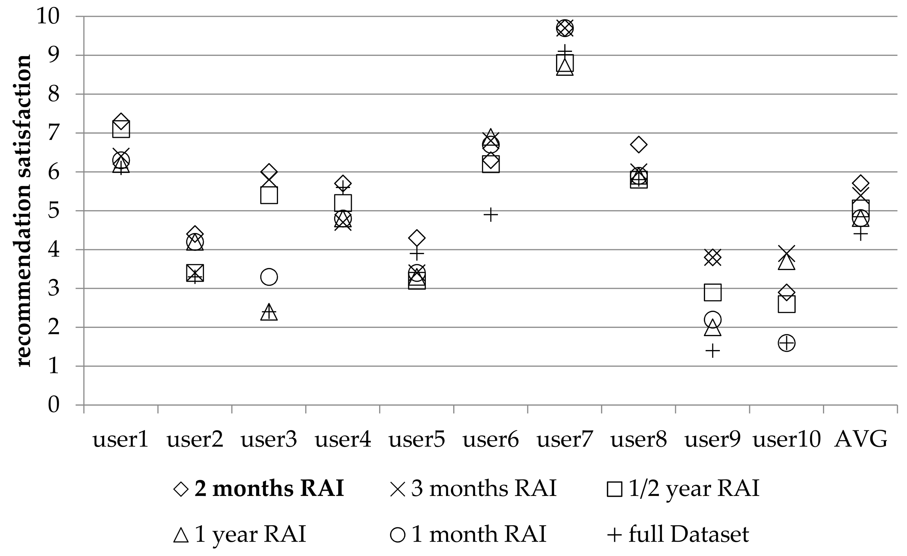
Figure 1 depicts the participants’ satisfaction from the recommended items, for all tested variants and the full dataset. The last column 1 (labeled as “AVG”) depicts the average score of all recommendations produced by the system. Regarding this average, can see that the two-month RAI variant achieves an overall score of 7.6, outperforming all the other RAI variants, as well as the full dataset. The runner up is the 3 month RAI, which scored an overall user satisfaction of 7.5 (or the 99% of the performance of the 2 month RAI, therefore closing the performance gap from the winner). The 1 month RAI variant was ranked third, the ½ year RAI was ranked fourth, the 1 year RAI variants ranked fifth and the full dataset was ranked sixth, with their performance being at the 96%, 93%, 88% and 84%, respectively, of the 2 month RAI variant, which was ranked first in this experiment. Overall, in more than 90% of the cases, the recommendation of the proposed algorithm using a RAI value of two months was ranked first or second (first: 76%, second: 15%; third: 7%). Note that when dropping ratings from a SN RS’s database, the influence levels between SN users change and so does the order of the influencers; hence the recommendations may be different in some cases.
Within Figure 1, we have the average ratings given by 10 individual users; these have been chosen to demonstrate that algorithm performance is not uniform across all users. In most occasions, the proposed technique with the optimal RAI variant produces the most favorably ranked recommendation, even at a tie with another algorithm.
To validate the significance of these results, we conducted statistical significance testing; the six rating prediction algorithms compared in Figure 1 were tested for statistical significance regarding the satisfaction reported by the users using the multivariate analysis of variance (MANOVA) statistical test; in the post-hoc tests, Bonferroni corrections were applied. The results of the post-hoc pairwise tests are illustrated in Table 1; for conciseness purposes, we include only the comparisons between the two best-performing RAI variants (2 months RAI and 3 months RAI).
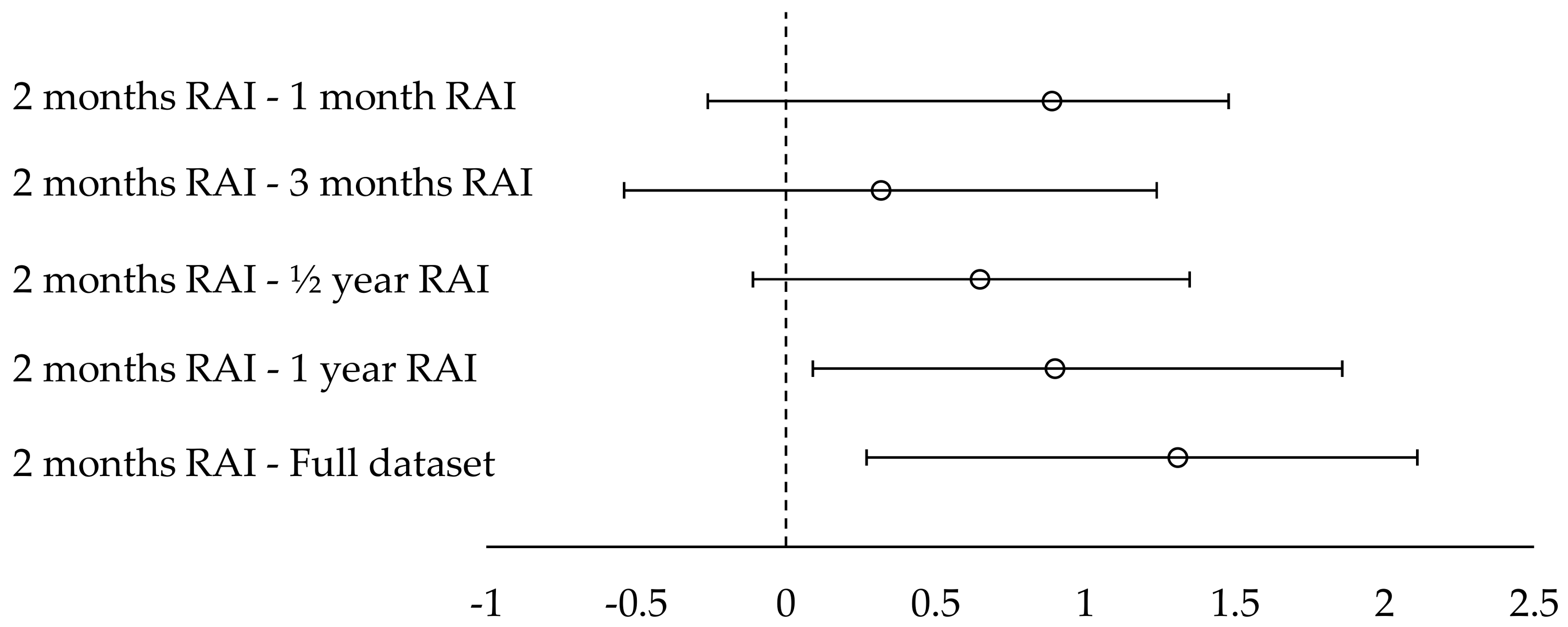
In Table 1 we can observe that the “2 month RAI” variant is established to have statistically significant superior performance with a confidence interval of 95% in comparison to the full dataset (i.e., the plain CF method) and the “1 year RAI” variant. On the contrary, statistical significance is not established for the variants “½ year RAI”, “3 month RAI” and “1 month RAI”, although the “2 month RAI” achieves a higher satisfaction average than these variants.
The runner up variant, “3 months RAI”, is shown to be statistically significant better with a confidence interval of 95% only comparison to the full dataset (i.e., the plain CF method).
Figure 2 illustrates the confidence intervals for the statistical significance tests between the best performing variant (“2 month RAI”) and other variants.
Overall, we can conclude that the consideration of RAI, according to the algorithm presented in Section 3, introduces a considerable (and statistically significant) improvement over the plain CF method, while the performance difference among different RAI settings varies, with the 2 month RAI setting having a performance edge.
4.1.2. User Satisfaction without Taking into Account the Items’ Categories
Since, as we stated in the introduction, the biggest advantage of CF is that explicit content description is not required (CF relies only on opinions expressed by users on items) we repeated the experiment, but without taking into account the categories that the items belong in. As far as the number of nearest neighbors taken into account per user, is concerned, this time we followed the work of Margaris et al. [9], where for each user we calculate his/her 30 strongest influencers where their influence level threshold ILth is larger than 0.18 (if less than 30 influencers with ILth > 0.18 are found, we keep only these ones; the threshold value of 0.18 is adopted from [9]). The computation of each user’s 30 (or less) strongest influencers was performed offline, following the work in [9].
Subsequently, each participant was presented with the top 10 items that attained the highest rating prediction from each of the variants considered in the first experiment and were asked to rate perceived satisfaction for each of the recommendations on a scale of 0 (totally unsatisfactory) to 10 (totally satisfactory). As noted above, however, the variants were modified to not utilize the category-specific influence levels. In this experiments, the items considered for recommendation were drawn from the set of 2000 items used in the first experiment. The order of presentation of the variants’ recommendations was again randomized, similarly to the first experiment. The cases when a particular item had been recommended by two or more variants were also handled in the same way as in the first experiment: again, the recommended item was presented only once to the subject and the score given by the subject was accounted for all the variants that produced the same recommendation.
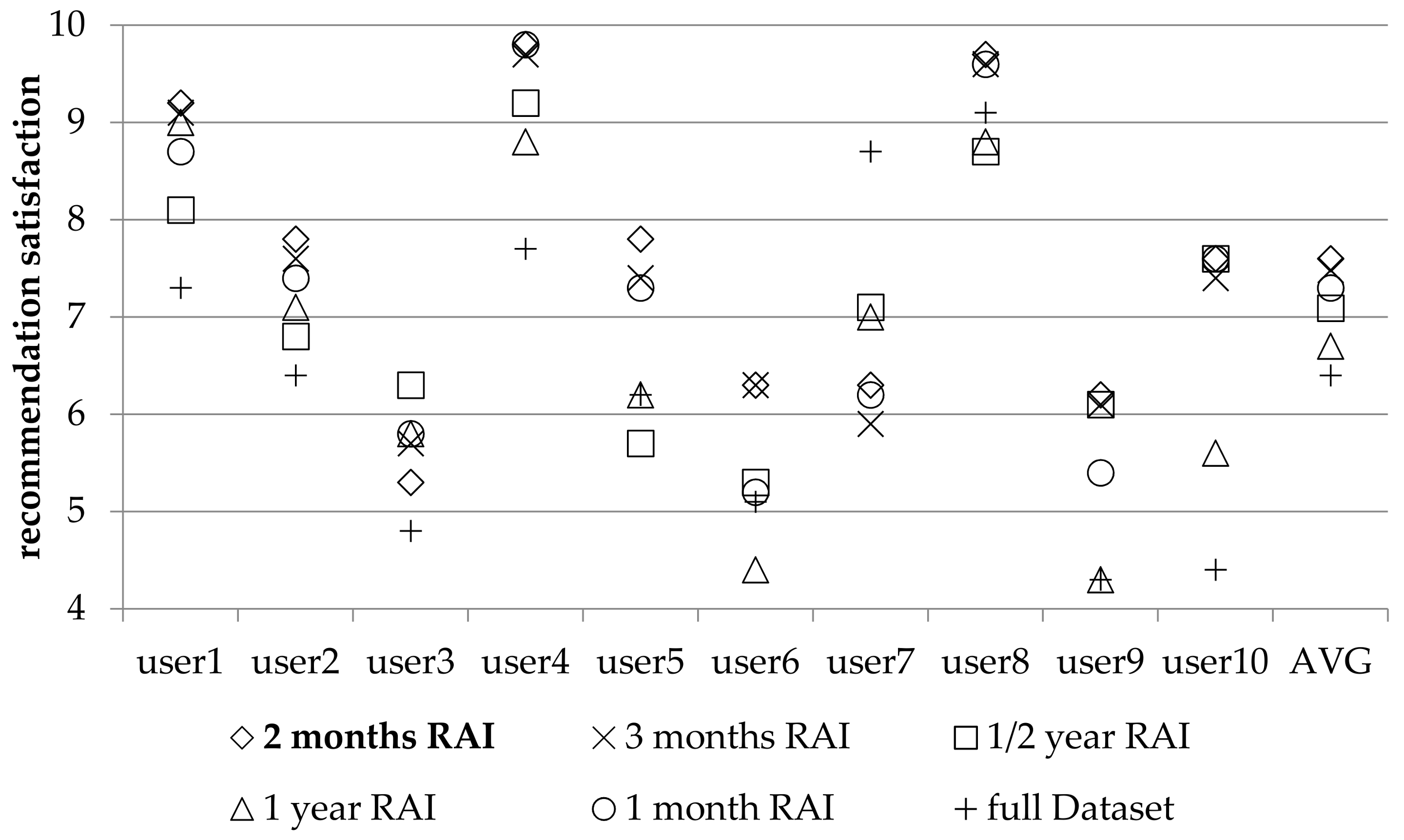
Figure 3 depicts the participants’ satisfaction from the recommended items, on a scale of 0 (totally unsatisfactory) to 10 (totally satisfactory), for different values of RAI and the initial datasets, when we do not take into account the items’ categories (genres of movies, types of books, etc.).
On average (last column on Figure 3; the average is calculated taking into account all satisfaction levels reported in this experiment, by all participating users) it is clear that the proposed technique using a RAI value of 2 months outperforms the other variants, as well as the full dataset, attaining an overall user satisfaction of 5.7. The runner up is the variant using a RAI value of 3 months, which scored an overall user satisfaction of 5.4 (or the 95% of the performance of the variant using a RAI value of 2 months). The ½ year RAI variant was ranked 3rd, while the 1 month and the 1 year RAI variants share the 4th position, and the full dataset was ranked 6th. The performance of the last four variants accounts for the 87%, 84% and 77%, respectively, of the 2 months RAI variant, which again performed best in this experiment. Again, within Figure 3 we have also included averages for 10 individual users; these have been chosen to demonstrate that algorithm performance is not perceived uniformly across all users. In most occasions, the proposed technique with the optimal RAI variant produces the most favorably ranked recommendation, even at a tie with another algorithm. It has to be noted, however, that in 85% of the cases, the recommendation of the proposed algorithm using a RAI value of 2 months was ranked first or second (first: 67%, second: 18%; third: 12%; fourth: 3%; fifth/sixth: none). We can also observe that all the recommendation scores are lower than the first experiment’s scores, due to the fact that influencers are not considered on a per-category basis, but rather as a generic level; this is consistent with the findings presented in Margaris et al. [8].
To validate the significance of these results, we conducted statistical significance testing; the six rating prediction algorithms compared in Figure 3 were tested for statistical significance regarding the satisfaction reported by the users using the MANOVA statistical test; in the post-hoc tests, Bonferroni corrections were applied. The results of the post-hoc pairwise tests are illustrated in Table 2; for conciseness purposes, we include only the comparisons between the two best-performing RAI variants (2 months RAI and 3 months RAI).
In the results illustrated in Table 2, we can observe that the improvement introduced by the “2 month RAI” variant is established to be statistically significant with a confidence interval of 95% against the full dataset (i.e., the plain CF method) as well as against the “1 year RAI” variant. On the contrary, statistical significance is not established for the variants “½ year RAI”, “3 month RAI”, and “1 month RAI” variants, as was also the case with the results of the first experiment. Again, the runner up variant, “3 months RAI”, is shown to be statistically significant better with a confidence interval of 95% only in comparison to the full dataset (i.e., the plain CF method).
Figure 4 illustrates the confidence intervals for the statistical significance tests between the best performing variant (“2 month RAI”) and other variants.
Overall, we can conclude that the consideration of RAI, according to the algorithm presented in Section 3, even without taking into account the product categories, introduces a considerable (and statistically significant) improvement over the plain CF method, while the performance difference among different RAI settings varies, with the 2 month RAI setting having a performance edge.
4.2. Evaluating the Proposed Technique Using RS’s Datasets
In order to generalize the proposed technique, we run a second set of experiments, using real datasets. More specifically, we used two datasets supplied by Amazon [42,43], as well as two datasets supplied by Movielens [44], which are widely used in RSs research. The Amazon datasets are sparse (from 0.0012% to 0.039%) and are simulating SN users having few ratings, while the Movielens datasets are relatively dense (from 0.54% to 5.88%), simulating SN users having a lot of ratings. The density of a dataset is defined as . As far as RS are concerned; regarding the notion of a “very sparse” dataset, we follow the definition of [48], where a dataset DS is deemed to be very sparse if for its density d(DS) it holds that d(DS) ≪ 1. These datasets contain “actual” timestamps (represented in UNIX format), i.e., timestamps entered in real rating time and not in a batch mode. In each dataset, users having less than 10 ratings were dropped, since users with few ratings are known to exhibit low accuracy in predictions computed for them [36]. Only the portion of the dataset which remained after pruning was considered during prediction formulation. The used datasets vary with respect to the date of publication (published from 1998 to 2016) and size (from 2 MB to 486 MB, in text format). The properties of these datasets are summarized in Table 3.
In this set of experiment, we added the RAI variants of 15 days, 10 days, 7 days, 5 days and 3 days, in order to further investigate smaller RAI variants. All newly introduced variants proved to be unsuccessful.
4.2.1. The Amazon “Videogames” Dataset
Table 4 depicts the results obtained from the Amazon “Videogames” dataset, concerning different values of RAI, before which all the users’ ratings are dropped.
Column “coverage” corresponds to the percentage of cases for which the CF algorithm could compute predictions (for some users, a prediction could not be formulated due to the “black sheep” phenomenon [49]: no recommendation can be produced for users having no neighbors with a positive Pearson coefficient [7,49], i.e., no candidate recommenders). Column “MAE” corresponds to the mean absolute error (MAE) of the predictions that were formulated when RAI was set to the corresponding value. Finally, column “dataset size (MB)/reduction%” indicates the rating database size, after the elimination of ratings in the preprocessing phase, as well as the percentage of reduction of the ratings database size achieved due to rating elimination, against the full database size. We note here that only the ratings which remained after the elimination phase were considered, both for user similarity computation and rating prediction.
Even when using the full dataset (the case denoted as “Full DB”), predictions could be formulated for only 71.93% of the cases; in the rest of them, the respective users had no candidate recommenders (neighbors with a positive Pearson coefficient [7,49]), and therefore no prediction could be computed for them.
We can observe that all RAI values achieve a MAE reduction when compared to the case of using the full database, and smaller values of RAI lead to higher reductions in MAE. However, smaller values of RAI also lead to decreased coverage, and consequently fewer users will be able to receive recommendations. In Table 4, we observe that if RAI is set to 3 days, coverage drops by 13.17%, which is a significant decrease.
Assuming that at most 5% of coverage drop is deemed tolerable (as suggested by Margaris and Vassilakis [34]), the optimal RAI value for this dataset is 10 days, which achieves a MAE reduction of 4.26%. We conducted a statistical significance test, comparing the ratings computed using the “10 days RAI” variant and those computed using the plain CF algorithm and the full dataset (the errors of the corresponding predictions were compared), and the differences observed have been shown to be statistically significant at confidence level 95% (p-value = 0.0483; t(99) = 11.6583, p < 0.05, d = 0.04). Statistical significance tests were conducted using paired t-tests [50], with each pair including the absolute errors corresponding to the two compared methods. Due to the nature of paired t-tests, only ratings that could be predicted by both algorithms were considered for the computation of statistical significance.
4.2.2. The Amazon “Books” Dataset
Table 5 depicts the results obtained from the Amazon “Books” dataset, for different values of RAI. The coverage obtained when using the full dataset is 86.9%. We can observe that all RAI values between 1 year and 10 days achieve a MAE reduction in relation to the case of using the full database, with the minimum MAE value achieved by all RAI values between 1 year and 30 days, with an acceptable amount of predictions being lost (from 0.64% to 0.79%) and a MAE reduction of 0.8%. We conducted a statistical significance test, comparing the ratings computed using the RAI variants producing the minimum MAE (i.e., the variants utilizing RAI values between 1 year and 30 days) and those computed using the plain CF algorithm and the full dataset, and the differences observed have not been shown to be statistically significant at confidence level 95% (p-value ranges between 0.0832 and 0.0854).
4.2.3. The MovieLens “Latest 20 M—Recommended for New Research” Dataset
Table 6 depicts the results obtained from the Amazon “Latest 20 M—recommended for new research” dataset, for different values of RAI. The coverage obtained when using the full dataset is 98.84%. We can observe that all the RAI variants achieve a MAE reduction in relation to the case of using the full database, with the minimum MAE value achieved when setting RAI to 3 days, where coverage drops by 0.25% and a reduction in the 2.99% on MAE is achieved. We conducted a statistical significance test, comparing the ratings computed using the “RAI 3 days” variant and those computed using the plain CF algorithm and the full dataset, and the differences observed have not been shown to be statistically significant at confidence level 95% (p-value = 0.0544).
4.2.4. The MovieLens “100 K” Dataset
Finally, Table 7 depicts the results obtained from the Amazon “100 K” dataset, for different values of RAI. The coverage obtained when using the full dataset is 97.67%. We can observe that all RAI values between 1 year and 30 days achieve a MAE reduction when compared to the case of using the full database, with the minimum MAE value being achieved when RAI is set to 60 days, with no predictions being lost (due to the dataset’s high density) and a MAE reduction of 3.02% being achieved. We conducted a statistical significance test, comparing the ratings computed using the “RAI 60 days” variant and those computed using the plain CF algorithm and the full dataset, and the differences observed have not been shown to be statistically significant at confidence level 95% (p-value = 0.0507).
4.2.5. Aggregate Statistics
In this Section we summarize and discuss our findings regarding the different RAI values used with the presented technique in the aforementioned datasets, exploring differences in MAE and coverage. In Table 8 we denote as “-”, if the RAI value (column) cannot be applied in the particular dataset (row), either because the MAE is larger than the initial dataset’s MAE (Full DB) or because the drop in coverage is greater than 5% and thus not considered as “tolerable” [34]; if a MAE reduction is achieved and coverage drops by less than 5%, then the RAI value is applicable and a “+” sign is noted.
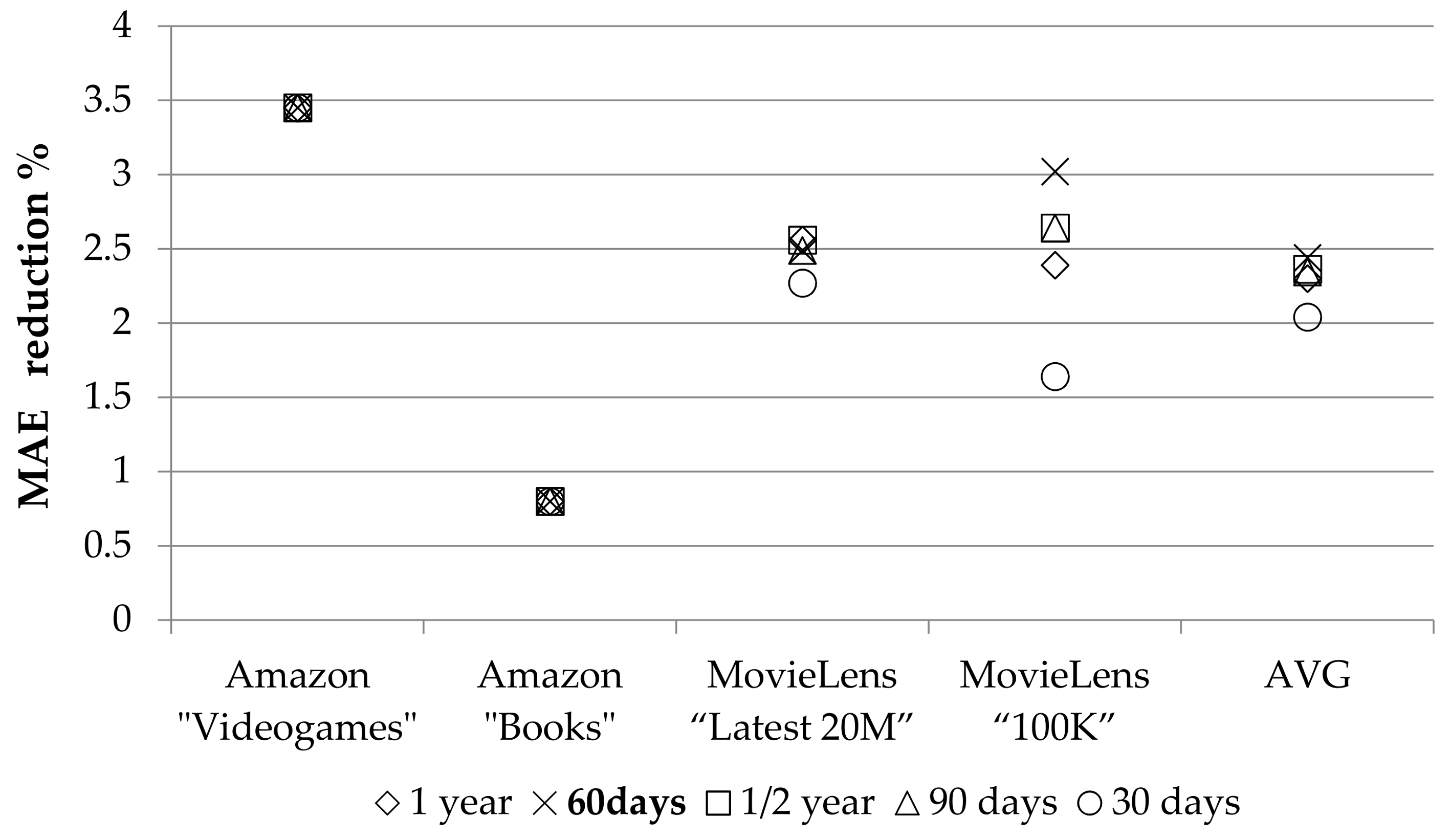
We can observe that the RAI values meeting both the MAE reduction (against the measurements obtained when using the initial, non-pruned database), as well as the coverage drop criteria in all cases are 1 year, ½ year, 90 days, 60 days and 30 days. Figure 5 compares these five variants with respect to MAE reduction in the four datasets tested.
On average (last column on Figure 5), the RAI value of 60 days outperforms all other candidate RAI values, attaining a MAE reduction average of 2.44%. The ½ year abstention interval comes in second with an average MAE reduction of 2.36%, or 96.7% of the reduction achieved by the value of 60 days. The 90 days RAI was ranked 3rd, the 1 year RAI was ranked fourth, and the 30 days RAI was ranked fifth, with average MAE reductions of 2.34%, 2.30% and 2.04%, respectively. Furthermore, the 60 days RAI was ranked first (or tied at first position) among the five RAI values considered in Figure 5 at three out of the four datasets tested, and third in only one case (MovieLens “Latest 20 M—recommended for new research”), where the RAI values of 1 year and ½ year achieved a 0.07% higher reduction in the MAE. Besides the benefits in the MAE reduction, the RAI value of 60 days achieves a rating database size decrement by 6.2% on average, due to the elimination of ratings from the ratings database.
4.3. Discussion
From the experiments presented in this Section, it is clear that using the proposed algorithm with a RAI value of 60 days achieves the optimal results as compared to other values of the RAI setting and also the plain CF algorithm; this has been verified in both the experiments measuring the satisfaction of real SN users, as well as in the experiments conducted using RSs’ datasets, with or without information about the items’ categories and under both dense and sparse datasets (a dataset is considered dense if SN users have entered many ratings on average; if SN users have entered few ratings, then the dataset is considered sparse), as well as using both SN metrics and traditional RSs metrics. This provides some evidence that an abstention of 60 days is likely to indicate that concept drift has occurred. Setting the abstention interval to a higher value renders the RS incapable of following the users’ interests, while the use of smaller values prunes useful ratings from the database, downgrading the performance of the RS.
As discussed in the literature review Section, other algorithms have been proposed insofar for handling the concept drift phenomenon and/or prune the ratings database, pursuing improvements in rating prediction accuracy. In the following, we present a comparison between the proposed approach and the pruning-based algorithms presented in [34,35]. Other results have also been published, however they are based on transient datasets (e.g., [12]) and/or employ different evaluation metrics (e.g., [11]), hindering direct comparison. It should be noted though that the proposed approach may be combined with deep learning approaches such as [11] or gradual forgetting algorithms [13]; in such combinations, the proposed approach may be used for preprocessing the dataset in order to prune ratings that are deemed to be not useful, while other techniques may then operate on the pruned dataset to generate rating predictions. In our future work, we plan to examine the effectiveness of such combinations.
Table 9 depicts the performance comparison between the proposed algorithm and the pruning-based algorithms presented in [34] and [35], namely “KeepLast” and “k-early”, respectively. The measurements regarding the performance of the “KeepLast” and “k-early” algorithms are sourced from the respective papers; the datasets listed in Table 9 are those for which measurements exist for all compared algorithms (i.e., the proposed one, “KeepLast” and “k-early”). In Table 9 we can observe that the proposed algorithm consistently achieves the highest MAE improvement, outperforming both “KeepLast” and “k-early” by a considerable margin (0.25% to 2.02%, and 0.97% on average from the runner-up, “k-early”). In terms of coverage drop, the proposed algorithm exhibits the minimum drop in two datasets and the second-to-minimum drop in the third dataset; in all cases, its performance regarding this metric is very close to that of “k-early” (the best performing under this measurement), lagging behind by a margin not exceeding 0.15% in any case, and only by 0.03% on average.
5. Conclusions and Future Research
In this paper we (1) established that when a SN user abstains from submitting ratings for a long time, it is a strong indication that concept drift has occurred and (2) presented a technique that exploits the abstention interval concept to drop ratings from the database, since these correspond to SN user preferences and likings that are not valid any more, due to the concept drift and shift of interest phenomena. By dropping invalidated ratings, database consistency is promoted, and this in turn leads to improved prediction quality.
We conducted two sets of experiments to test different values of the RAI parameter ranging from 3 days to 1 year, using real SN users, as well as, widely acceptable RSs’ datasets, using SN metrics and traditional RSs metrics, respectively, and compared the different RAI values considering (1) users’ satisfaction, (2) prediction accuracy and (3) predictions coverage. The results show that the optimal value for the rating abstention interval lies around 60 days, where the user satisfaction is maximized (+19% on average, when comparing it to the full ratings dataset), when evaluating real SN users’ satisfaction, and an average of 2.44% MAE reduction is achieved, with coverage dropping by only 0.425% on average, when testing the RSs’ datasets.
A merit of the suggested rating elimination technique is that it can be applied as a preprocessing step to any CF-based algorithm.
Regarding our future work, we plan to investigate more rating abstention interval values, especially variants which are close to the optimal value found in this paper, as well as setting different rating abstention interval for different users. We also plan to evaluate our technique with more rating prediction algorithms, such as matrix factorization [51].
Author Contributions
All authors conceived, designed and performed the experiments; analyzed the data and wrote the paper.
Conflicts of Interest
The authors declare no conflict of interest.
References
- Facebook Home Page. Available online: https://www.facebook.com (accessed on 5 January 2018).
- Twitter Home Page. Available online: https://twitter.com/ (accessed on 5 January 2018).
- Bakshy, E.; Eckles, D.; Yan, R.; Rosenn, I. Social influence in social advertising: Evidence from field experiments. In Proceedings of the 13th ACM Conference on Electronic Commerce, Valencia, Spain, 4–8 June 2012. [Google Scholar]
- Margaris, D.; Vassilakis, C.; Georgiadis, P. Knowledge-based leisure time recommendations in social networks. In Current Trends on Knowledge-Based Systems: Theory and Applications; Alor-Hernández, G., Valencia-García, R., Eds.; Intelligent Systems Reference Library, Springer: Cham, Switzerland, 2017. [Google Scholar]
- Arazy, O.; Kumar, N.; Shapira, B. Improving social recommender systems. IT Prof. 2009, 11, 38–44. [Google Scholar] [CrossRef]
- Schafer, J.B.; Frankowski, D.; Herlocker, J.; Sen, S. Collaborative Filtering Recommender Systems. In The Adaptive Web; Brusilovsky, P., Kobsa, A., Nejdl, W., Eds.; Springer: Berlin, Germany, 2007. [Google Scholar]
- Balabanovic, M.; Shoham, Y. Fab: Content-based, collaborative recommendation. Commun. ACM 1997, 40, 66–72. [Google Scholar] [CrossRef]
- Margaris, D.; Vassilakis, C.; Georgiadis, P. Recommendation information diffusion in social networks considering user influence and semantics. Soc. Netw. Anal. Min. 2016, 6, 1–22. [Google Scholar] [CrossRef]
- Margaris, D.; Vassilakis, C.; Georgiadis, P. Query personalization using social network information and collaborative filtering techniques. Futur. Gener. Comput. Syst. 2018, 78, 440–450. [Google Scholar] [CrossRef]
- Gilbert, E.; Karahalios, K. Predicting tie strength with social media. In Proceedings of the SIGCHI Conference on Human Factors in Computing Systems (CHI ‘09), Boston, MA, USA, 4–9 April 2009. [Google Scholar]
- Song, Y.; Elkahky, A.; He, X. Multi-rate deep learning for temporal recommendation. In Proceedings of the 39th International ACM SIGIR Conference on Research and Development in Information Retrieval, Pisa, Italy, 17–21 July 2016. [Google Scholar]
- Li, L.; Zheng, L.; Yang, F.; Li, T. Modeling and broadening temporal user interest in personalized news recommendation. Expert Syst. Appl. 2014, 41, 3168–3177. [Google Scholar] [CrossRef]
- Gama, J.; Žliobaitė, I.; Bifet, A.; Pechenizkiy, M.; Bouchachia, A. A survey on concept drift adaptation. ACM Comput. Surv. 2014, 46. [Google Scholar] [CrossRef]
- Gama, J. Knowledge Discovery from Data Streams, 1st ed.; Chapman & Hall/CRC: London, UK, 2010. [Google Scholar]
- Zliobaite, I. Adaptive Training Set Formation. Ph.D. Thesis, Vilnius University, Vilnius, Lithuania, 2010. [Google Scholar]
- Bakshy, E.; Rosenn, I.; Marlow, C.; Adamic, L. The role of social networks in information diffusion. In Proceedings of the 21st International Conference on World Wide Web, Lyon, France, 16–20 April 2012. [Google Scholar]
- Oechslein, O.; Hess, T. The value of a recommendation: The role of social ties in social recommender systems. In Proceedings of the 47th Hawaii International Conference on System Science, Waikoloa, HI, USA, 6–9 January 2014. [Google Scholar]
- Gulcin, O.M.; Polat, F. Trust based recommendation systems. In Proceedings of the IEEE/ACM International Conference on Advances in Social Networks Analysis and Mining (ASONAM 2016), Niagara Falls, ON, Canada, 25–28 August 2013. [Google Scholar]
- Fotia, L.; Messina, F.; Rosaci, D.; Sarné, G. Using local trust for forming cohesive social structures in virtual communities. Comput. J. 2017, 60, 1717–1727. [Google Scholar] [CrossRef]
- Martinez-Cruz, C.; Porcel, C.; Bernabé-Moreno, J.; Herrera-Viedma, E. A model to represent users trust in recommender systems using ontologies and fuzzy linguistic modeling. Inf. Sci. Int. J. 2015, 311, 102–118. [Google Scholar] [CrossRef]
- Walter, F.E.; Battiston, S.; Schweitzer, F.A. Model of a trust-based recommendation system on a social network. Auton. Agents Multi-Agent Syst. 2008, 16, 57–74. [Google Scholar] [CrossRef]
- O’Donovan, J.; Smyth, B. Trust in recommender systems. In Proceedings of the 10th International Conference on Intelligent User Interfaces (ACM IUI ‘05), San Diego, CA, USA, 10–13 January 2005. [Google Scholar]
- Bedi, P.; Kaur, H.; Marwaha, S. Trust based recommender system for the semantic web. In Proceedings of the 20th International Joint Conference on Artificial intelligence (IJCAI ‘07), Hyderabad, India, 6–12 January 2007. [Google Scholar]
- Rosaci, D. Finding semantic associations in hierarchically structured groups of Web data. Form. Asp. Comput. 2015, 27, 867–884. [Google Scholar] [CrossRef]
- Cabrera Rivera, L.; Vilches-Blázquez, L.M.; Torres-Ruiz, M.; Moreno Ibarra, M.A. Semantic Recommender System for Touristic Context Based on Linked Data. In Information Fusion and Geographic Information Systems (IF&GIS’ 2015); Popovich, V., Claramunt, C., Schrenk, M., Korolenko, K., Gensel, J., Eds.; Springer: Cham, Switzerland, 2015; pp. 77–89. [Google Scholar]
- Adomavicius, G.; Tuzhilin, A. Context-aware recommender systems. In Proceedings of the 2008 ACM Conference on Recommender Systems (RecSys ‘08), Lausanne, Switzerland, 23–25 October 2008. [Google Scholar]
- Liu, X.; Aberer, K. SoCo: A social network aided context-aware recommender system. In Proceedings of the 22nd International Conference on World Wide Web (WWW ‘13), Rio de Janeiro, Brazil, 13–17 May 2013. [Google Scholar]
- Tsymbal, A. The Problem of Concept Drift: Definitions and Related Work; Computer Science Department, Trinity College: Dublin, Ireland, 2004. [Google Scholar]
- Stanley, K.O. Learning Concept Drift with a Committee of Decision Trees; Technology Report UTAI-TR-03–302; Department of Computer Sciences, University of Texas: Austin, TX, USA, 2003. [Google Scholar]
- Brzezinski, D.; Stefanowski, J. Reacting to different types of concept drift: The accuracy updated ensemble algorithm. IEEE Trans Neural Netw. Learn. Syst. 2014, 25, 81–94. [Google Scholar] [CrossRef] [PubMed]
- Ning, L.; Zhang, G.; Lu, J. Concept drift detection via competence models. Artif. Intell. 2014, 209, 11–28. [Google Scholar]
- Liu, A.; Zhang, G.; Lu, J. Concept drift detection based on anomaly analysis. In Proceedings of the 21st International Conference on Neural Information Processing (ICONIP 2014), Kuching, Malaysia, 3–6 November 2014. [Google Scholar]
- Shao, J.; Ahmadi, Z.; Kramer, S. Prototype-based learning on concept-drifting data streams. In Proceedings of the ACM SIGKDD International Conference on Knowledge Discovery and Data Mining (KDD ‘14), New York, NY, USA, 24–27 August 2014. [Google Scholar]
- Margaris, D.; Vassilakis, C. Pruning and aging for user histories in collaborative filtering. In Proceedings of the IEEE Symposium Series on Computational Intelligence (SSCI 2016), Athens, Greece, 6–9 December 2016. [Google Scholar]
- Margaris, D.; Vassilakis, C. Enhancing User Rating Database Consistency through Pruning. In Transactions on Large-Scale Data- and Knowledge-Centered Systems XXXIV; Hameurlain, A., Küng, J., Wagner, R., Decker, H., Eds.; Springer: Berlin, Germany, 2017. [Google Scholar]
- Ekstrand, M.D.; Riedl, J.T.; Konstan, J.A. Collaborative filtering recommender systems. Found. Trends Hum. Comput. Interact. 2011, 4, 81–173. [Google Scholar] [CrossRef]
- Charness, G.; Gneezy, U.; Kuhn, M.A. Experimental methods: Between-subject and within-subject design. J. Econom. Behav. Organ. 2012, 18. [Google Scholar] [CrossRef]
- Within-Subjects Designs. Available online: https://web.mst.edu/~psyworld/within_subjects.htm (accessed on 25 April 2018).
- Facebook Interest Targeting. Available online: https://www.facebook.com/help/188888021162119 (accessed on 25 April 2018).
- Google Interests. Available online: https://support.google.com/ads/answer/2842480 (accessed on 25 April 2018).
- Herlocker, J.; Konstan, J.; Terveen, L.; Riedl, J. Evaluating collaborative filtering recommender systems. ACM Trans. Inf. Syst. 2004, 22, 5–53. [Google Scholar] [CrossRef]
- Amazon Product Data. Available online: http://jmcauley.ucsd.edu/data/amazon/links.html (accessed on 11 January 2018).
- McAuley, J.; Targett, C.; Shi, Q.; Van den Hengel, A. Image-based recommendations on styles and substitutes. In Proceedings of the 38th International ACM SIGIR Conference on Research and Development in Information Retrieval (SIGIR ‘15), Santiago, Chile, 9–13 August 2015. [Google Scholar]
- MovieLens Datasets. Available online: http://grouplens.org/datasets/movielens/ (accessed on 26 January 2018).
- Facebook Graph API. Available online: https://developers.facebook.com/docs/graph-api (accessed on 17 November 2017).
- Facebook, Anatomy of Facebook. Available online: https://www.facebook.com/notes/facebook- data-science/anatomy-of-facebook/10150388519243859/ (accessed on 17 November 2017).
- Amazon Product Advertising API. Available online: https://docs.aws.amazon.com/AWSECommerceService/latest/DG/Welcome.html (accessed on 25 April 2018).
- Pan, R.; Zhou, Y.; Cao, B.; Liu, N.N.; Lukose, R.; Scholz, M.; Yang, Q. One-class collaborative filtering. In Proceedings of the 8th IEEE International Conference on Data Mining (ICDM), Pisa, Italy, 15–19 December 2008. [Google Scholar]
- Burke, R. Hybrid recommender systems: Survey and experiments. User Model. User Adapt. Interact. 2002, 12, 331–370. [Google Scholar] [CrossRef]
- Hsu, H.; Lachenbruch, P.A. Paired t Test. In Wiley StatsRef: Statistics Reference Online; Balakrishnan, N., Colton, T., Everitt, B., Piegorsch, W., Ruggeri, F., Teugels, J.L., Eds.; Willey: Hoboken, NJ, USA, 2014. [Google Scholar]
- Koren, Y.; Bell, R.; Volinsky, C. Matrix factorization techniques for recommender systems. Computer 2009, 42, 30–37. [Google Scholar] [CrossRef]
Figure 1.
Users’ satisfaction of recommendations made using different RAI variants, when taking into account users’ influencers per category.
Figure 1.
Users’ satisfaction of recommendations made using different RAI variants, when taking into account users’ influencers per category.

Figure 2.
95% confidence intervals for the statistical significance tests between the best performing variant (“2 month RAI”) and other variants.
Figure 2.
95% confidence intervals for the statistical significance tests between the best performing variant (“2 month RAI”) and other variants.

Figure 3.
Users’ satisfaction of recommendations made using different RAI variants, without taking into account users’ influencers per category, in the context of the second experiment.
Figure 3.
Users’ satisfaction of recommendations made using different RAI variants, without taking into account users’ influencers per category, in the context of the second experiment.

Figure 4.
95% confidence intervals for the statistical significance tests between the best performing variant (“2 month RAI”) and other variants, in the context of the second experiment.
Figure 4.
95% confidence intervals for the statistical significance tests between the best performing variant (“2 month RAI”) and other variants, in the context of the second experiment.

Figure 5.
MAE reduction achieved by the different RAI values on the 4 different datasets (baseline: MAE of non-pruned database, without application of RAI).
Figure 5.
MAE reduction achieved by the different RAI values on the 4 different datasets (baseline: MAE of non-pruned database, without application of RAI).


Table 1.
Statistical significance tests for the results of the first experiment.
| First Algorithm | Second Algorithm | Mean Difference | Significance | Statistically Significant at p < 0.05? |
|---|---|---|---|---|
| 2 months RAI | 1 month RAI | 0.89 | 0.1368 | No |
| 3 months RAI | 0.32 | 0.1832 | No | |
| ½ year RAI | 0.65 | 0.0583 | No | |
| 1 year RAI | 0.90 | 0.0461 | Yes | |
| Full dataset | 1.31 | 0.0309 | Yes | |
| 3 months RAI | 1 month RAI | 0.58 | 0.1736 | No |
| 2 months RAI | −0.32 | 0.1832 | No | |
| ½ year RAI | 0.33 | 0.0811 | No | |
| 1 year RAI | 0.58 | 0.0553 | No | |
| Full dataset | 0.98 | 0.0375 | Yes |
Table 2.
Statistical significance tests for the results of the first experiment.
| First Algorithm | Second Algorithm | Mean Difference | Significance | Statistically Significant at p < 0.05? |
|---|---|---|---|---|
| 2 months RAI | 1 month RAI | 0.30 | 0.1732 | No |
| 3 months RAI | 0.12 | 0.3473 | No | |
| ½ year RAI | 0.52 | 0.0603 | No | |
| 1 year RAI | 0.92 | 0.0483 | Yes | |
| Full dataset | 1.19 | 0.0354 | Yes | |
| 3 months RAI | 1 month RAI | 0.18 | 0.2912 | No |
| 2 months RAI | −0.12 | 0.3473 | No | |
| ½ year RAI | 0.39 | 0.2139 | No | |
| 1 year RAI | 0.78 | 0.5154 | No | |
| Full dataset | 1.08 | 0.0389 | Yes |
Table 3.
Datasets summary.
| Dataset Name | #Users | #Items | #Ratings | Avg. #Ratings/User | DB Size (in Text Format) |
|---|---|---|---|---|---|
| Amazon “Videogames” [42,43] | 8 K | 50 K | 157 K | 19.6 | 3.6 MB |
| Amazon “Books” [42,43] | 295 K | 2.3 M | 8.7 M | 29.4 | 227 MB |
| MovieLens “Latest Datasets—20 M—recommended for new research” [44] | 138 K | 27 K | 20 M | 145 | 486 MB |
| MovieLens “100 K” [44] | 1 K | 1.7 K | 100 K | 100 | 2 MB |
Table 4.
Amazon “Videogames” dataset results.
| RAI | % Coverage | MAE (out of 4) | Dataset Size (MB)/Reduction % |
|---|---|---|---|
| Full DB | 71.93 | 0.869 | 3.55/0.0% |
| 1 year | 70.81 | 0.839 | 3.37/5.1% |
| ½ year | 70.81 | 0.839 | 3.37/5.1% |
| 90 days | 70.81 | 0.839 | 3.37/5.1% |
| 60 days | 70.81 | 0.839 | 3.37/5.1% |
| 30 days | 70.75 | 0.839 | 3.36/5.4% |
| 15 days | 69.88 | 0.834 | 3.30/7.0% |
| 10 days | 68.46 | 0.832 | 3.20/9.9% |
| 7 days | 66.14 | 0.829 | 3.00/15.5% |
| 5 days | 63.66 | 0.815 | 2.84/20.0% |
| 3 days | 58.76 | 0.812 | 2.47/30.4% |
Table 5.
Amazon “Books” dataset results.
| RAI | % Coverage | MAE (out of 4) | Dataset Size (MB)/Reduction % |
|---|---|---|---|
| Full DB | 86.90 | 0.755 | 232/0.0% |
| 1 year | 86.26 | 0.749 | 211/9.1% |
| ½ year | 86.26 | 0.749 | 211/9.1% |
| 90 days | 86.26 | 0.749 | 211/9.1% |
| 60 days | 86.26 | 0.749 | 211/9.1% |
| 30 days | 86.11 | 0.749 | 210/9.5% |
| 15 days | 85.06 | 0.752 | 202/12.9% |
| 10 days | 83.86 | 0.754 | 191/17.7% |
| 7 days | 82.53 | 0.759 | 180/22.4% |
| 5 days | 81.19 | 0.761 | 167/28.0% |
| 3 days | 78.95 | 0.766 | 147/36.6% |
Table 6.
MovieLens “latest 20 M—recommended for new research” dataset results.
| RAI | % Coverage | MAE (out of 9) | Dataset Size (MB)/Reduction % |
|---|---|---|---|
| Full DB | 98.84 | 1.407 | 467/0.0% |
| 1 year | 98.83 | 1.371 | 444/4.9% |
| ½ year | 98.83 | 1.371 | 443/5.1% |
| 90 days | 98.82 | 1.372 | 437/6.4% |
| 60 days | 98.83 | 1.372 | 431/7.7% |
| 30 days | 98.82 | 1.375 | 415/11.1% |
| 15 days | 98.67 | 1.380 | 394/15.6% |
| 10 days | 98.59 | 1.382 | 381/18.4% |
| 7 days | 98.66 | 1.379 | 370/20.8% |
| 5 days | 98.69 | 1.370 | 361/22.7% |
| 3 days | 98.59 | 1.365 | 349/25.3% |
Table 7.
MovieLens “100 K” dataset results.
| RAI | % Coverage | MAE (out of 4) | Dataset Size (MB)/Reduction % |
|---|---|---|---|
| Full DB | 97.67 | 0.795 | 2.04/0.0% |
| 1 year | 97.67 | 0.776 | 2.02/1.0% |
| ½ year | 97.67 | 0.774 | 2.02/1.0% |
| 90 days | 97.67 | 0.774 | 1.98/2.9% |
| 60 days | 97.67 | 0.771 | 1.98/2.9% |
| 30 days | 97.67 | 0.782 | 1.89/7.4% |
| 15 days | 97.45 | 0.801 | 1.83/10.3% |
| 10 days | 97.56 | 0.809 | 1.79/12.3% |
| 7 days | 97.67 | 0.809 | 1.74/14.7% |
| 5 days | 97.88 | 0.814 | 1.71/16.2% |
| 3 days | 97.45 | 0.807 | 1.67/18.1% |
Table 8.
RAI variants comparison.
| RAI Value | ||||||||||
|---|---|---|---|---|---|---|---|---|---|---|
| Dataset Name | 1 Year | ½ Year | 90 Days | 60 Days | 30 Days | 15 Days | 10 Days | 7 Days | 5 Days | 3 Days |
| Amazon “Videogames” | + | + | + | + | + | + | + | - | - | - |
| Amazon “Books” | + | + | + | + | + | + | + | - | - | - |
| MovieLens “Latest 20 M” “recommended for new research” | + | + | + | + | + | + | + | + | + | + |
| MovieLens “100 K” | + | + | + | + | + | - | - | - | - | - |
Table 9.
RAI variants comparison.
| Dataset Name | MAE Improvement | Coverage Drop | ||||
|---|---|---|---|---|---|---|
| KeepLast [34] | k-Early [35] | Proposed | KeepLast [34] | k-Early [35] | Proposed | |
| Amazon “Videogames” | 1.10% | 3.20% | 3.45% | 3.43% | 1.40% | 1.55% |
| MovieLens “Latest 20 M” “recommended for new research” | 0.02% | 1.87% | 2.49% | 0.90% | 0.01% | 0.01% |
| MovieLens “100 K” | 0.32% | 1.00% | 3.02% | 0.81% | 0.06% | 0.00% |
| Average | 0.48% | 2.02% | 2.99% | 1.71% | 0.49% | 0.52% |
© 2018 by the authors. Licensee MDPI, Basel, Switzerland. This article is an open access article distributed under the terms and conditions of the Creative Commons Attribution (CC BY) license (http://creativecommons.org/licenses/by/4.0/).
Share and Cite
MDPI and ACS Style
Margaris, D.; Vassilakis, C. Exploiting Rating Abstention Intervals for Addressing Concept Drift in Social Network Recommender Systems. Informatics 2018, 5, 21. https://doi.org/10.3390/informatics5020021
AMA Style
Margaris D, Vassilakis C. Exploiting Rating Abstention Intervals for Addressing Concept Drift in Social Network Recommender Systems. Informatics. 2018; 5(2):21. https://doi.org/10.3390/informatics5020021
Chicago/Turabian StyleMargaris, Dionisis, and Costas Vassilakis. 2018. "Exploiting Rating Abstention Intervals for Addressing Concept Drift in Social Network Recommender Systems" Informatics 5, no. 2: 21. https://doi.org/10.3390/informatics5020021
Note that from the first issue of 2016, this journal uses article numbers instead of page numbers. See further details here.