Building Realistic Mobility Models for Mobile Ad Hoc Networks


School of Computing, Creative Technologies, Leeds Beckett University, Headingley Campus, Leeds LS6 3QS, UK
*
Author to whom correspondence should be addressed.
Informatics 2018, 5(2), 22; https://doi.org/10.3390/informatics5020022
Submission received: 8 February 2018
/
Revised: 17 April 2018
/
Accepted: 23 April 2018
/
Published: 30 April 2018
Abstract
:A mobile ad hoc network (MANET) is a self-configuring wireless network in which each node could act as a router, as well as a data source or sink. Its application areas include battlefields and vehicular and disaster areas. Many techniques applied to infrastructure-based networks are less effective in MANETs, with routing being a particular challenge. This paper presents a rigorous study into simulation techniques for evaluating routing solutions for MANETs with the aim of producing more realistic simulation models and thereby, more accurate protocol evaluations. MANET simulations require models that reflect the world in which the MANET is to operate. Much of the published research uses movement models, such as the random waypoint (RWP) model, with arbitrary world sizes and node counts. This paper presents a technique for developing more realistic simulation models to test and evaluate MANET protocols. The technique is animation, which is applied to a realistic scenario to produce a model that accurately reflects the size and shape of the world, node count, movement patterns, and time period over which the MANET may operate. The animation technique has been used to develop a battlefield model based on established military tactics. Trace data has been used to build a model of maritime movements in the Irish Sea. Similar world models have been built using the random waypoint movement model for comparison. All models have been built using the ns-2 simulator. These models have been used to compare the performance of three routing protocols: dynamic source routing (DSR), destination-sequenced distance-vector routing (DSDV), and ad hoc n-demand distance vector routing (AODV). The findings reveal that protocol performance is dependent on the model used. In particular, it is shown that RWP models do not reflect the performance of these protocols under realistic circumstances, and protocol selection is subject to the scenario to which it is applied. To conclude, it is possible to develop a range of techniques for modelling scenarios applicable to MANETs, and these simulation models could be utilised for the evaluation of routing protocols.
1. Introduction
This paper is an extension of Pullin and Pattinson (2008) [1], which discusses a battlefield model based on a real building and current military tactics, and extracted from PhD research by Pullin (2014) [2]. Whilst many early computer networks relied on wired connections, the use of wireless radio in data communications has been at the forefront of research since the 1960s, such as with the Aloha network that was developed at the University of Hawaii (Abramson, 1970, [3]) and provided a number of the concepts implemented in Ethernet (Metcalfe and Boggs, 1976, [4]). The cycle of development repeated itself as the size of computing devices has reduced to such an extent that portable computers are possible. The flexibility of portable computers is reduced considerably if they have to be plugged in, using a cable, in order to access networking facilities; so, again, wireless radio technology is developed, largely in the form of wireless Ethernet (IEEE, 2013, [5]). This allows a computer—which is taken to refer to a broad range of devices, from small handheld smart phones to desktop personal computers (PCs) and increasingly, to consumer devices, such as smart TVs—to connect to a local area network without being tethered by a network cable.
The advent of mobile phones and in particular, their development into smart phones has resulted in another networking paradigm, whereby the device connects wirelessly to a telecommunications network, these days through 3G, increasingly 4G (ITU, 2010, [6]), and emerging 5G technologies, which will be deployed between 2020 and 2030 (HuaWei, 2013, [7]). The convergence of mobile phone and computer technology now means that there is a blurring of devices, such that clear distinctions between phones, tablet devices, netbooks, laptop computers, games consoles, televisions (TVs), etc. are no longer possible. All these devices are computers and can communicate via networks, predominantly using one of the previously mentioned wireless technologies. These wireless technologies allow a significant amount of device mobility and portability. Movement within the range of a wireless access point or a specific mobile telephone mast is trivial, and roving between access points or masts is straightforward, at least from a user’s point of view. Thus, the concept of mobile computing emerges.
One thing that links all of these devices and networks, both in terms of data communications and operational paradigm, is the reliance on an existing wireless infrastructure to which they can connect. This last hop link is known as the “last segment of end to end performance from a server to an end user device, which includes any Wi-Fi network at home, business, or public Wi-Fi hotspot, etc.” (Badu Networks, 2016, [8]). It provides a significant degree of flexibility over a cable, but it is dependent on there being a pre-installed local area network (for wireless Ethernet) or telecommunications network (for 3G, 4G, and 5G). This reliance on pre-configured networks is satisfactory in many cases and has resulted in existing network infrastructures. However, the deployment and management of network infrastructures could be complex, costly, and time consuming (Computerworld, 2011, [9]). Such solutions could be vulnerable to failure caused by natural disasters, accidental, or deliberate interference. Therefore, there do arise circumstances where traditional pre-installed networking systems are not available. Examples are disaster zones, where the networking infrastructure has been destroyed, and battlefields, where there is insufficient time to deploy an infrastructure. In such cases, a networking solution is required that does not rely on anything pre-installed at all, and this leads to the concept of mobile ad hoc networks (Johnson and Maltz, 1996, [10]).
A mobile ad hoc network (MANET) is an emerging type of wireless networking where mobile nodes associate on an extemporaneous or ad hoc basis (Cisco, nd, [11]). It comprises a collection of mobile computers that communicate with each other via a self-organising, self-forming, self-healing communication network, without reliance on fixed infrastructures or centralised control or resources (Johnson and Maltz, 1996, [10]). Within a MANET, each computer or node has the potential to act as a data source, a data sink, and/or a router. The nature of each computer is not generally important as long as it can support the stated aspects of the MANET. MANET research predates modern developments in mobile devices and in particular, Wireless Local Area Network (LAN) (IEEE 802.11/Wi-Fi). Details of IEEE 802.11™ (Wireless LANs) are found here (IEEE, 2016, [12]). Wireless networking technologies now allow a heterogeneous collection of devices, which have compatible communications technology, such as 802.11, to be formed into a MANET. Much research that has been conducted on IEEE 802.11-based MANET address the following issues: power management protocols (Tseng et al., 2003, [13]); development of multicast aware MAC protocol (Gossain et al., 2004, [14]) followed by improvement of the MAC protocol (Dureja et al., 2010, [15]) and adaptive MAC 802.11 protocol (Patheja et al., 2013, [16]); development of a scalable and adaptive clock synchronization protocol. However, the development of MANET technology presents a range of challenges that are the subject of extensive research.
1.1. Problem Statement
The development of simulations plays a vital role in Mobile Ad Hoc Network (MANET)-related research. All aspects of the simulation need to be as realistic as possible for it to provide valid and meaningful data. Any aspect of the simulation model will lead to significant research questions. This research does not consider the following: radio propagation models, the implementation of protocols, power consumption, or security issues. There are significant differences in the performance results of simulations due to variations in the world models used. Many MANET protocol studies still employ basic simulation models with little or no relevance to the common, real-world applications cited for mobile ad hoc networks. In order to facilitate transferability to the real world, it is necessary to employ robust and realistic simulations of real-world scenarios for the evaluation of protocols. Realistic MANET simulations add soundness and credibility to evaluations of MANET routing protocols (Cavilla et al., 2004, [17]; Munjal et al., 2010, [18]); they produce vastly different results compared to commonly used simplistic models (Sommer et al., 2007, [19]) and will lead to real deployments (Lan and Chou, 2008, [20]). This research article addresses three important aspects for the development of a world model: simulation time, node count, and movement aspects of realistic models. They form the bases for the measures used for the evaluation of the model. The techniques and models presented here could be applied to research areas where mobility models are necessary, though issues addressed in this research are closely related to MANET. The main contribution of this work is to provide researchers access to models that facilitate easy construction of rigorous MANET simulation scenarios. The input to our models consists of desired values for the three previously mentioned measures. Subsequently, our models output parameters for a simulation scenario that approximately meets the benchmarks. Our first MANET model is designed based on a human movement mobility model (e.g., Musolesi and Muscolo, 2006, [21]; Papargeorgiou et al., 2012, [22]). The second model is a shipping model based on maritime movements in the Irish Sea. To reiterate, our models enable researchers to test MANET routing protocols in a more realistic manner, thereby improving the credibility of their MANET simulation studies.
1.2. Research Aim
The main aim of this research is to develop new techniques for producing realistic mobility and world models that could be used to evaluate MANET protocols in two different contexts: modelled battlefield and shipping movement. Its other goal is to show that different MANET application scenarios require different routing protocols. This is demonstrated by the fact that these realistic models yield significantly different results from commonly used simulation models, such as the random waypoint model (RWP). Their performance also varies when applied to common protocols. Thus, there is no single solution to the MANET routing problem, and different application areas will have different suitable protocols.
2. Literature Review
The literature reviewed in this paper encompasses the following: MANET, its operations, applications, performance evaluation, and nS-2 to simulate MANET routing algorithms.
2.1. Mobile Ad Hoc Network (MANET)
The development of mobile ad hoc networks can be traced back to projects run by the American Defence Advanced Research Projects Agency (DARPA) in the 1970s, when packet radio systems (PRNET) are developed to carry Advanced Research Projects Agency Network (ARPANET) between fixed and mobile nodes (Jubin and Tornow, 1987, [23]). A key focus in MANET has been the routing problem, and a large number of routing protocols have been proposed: destination-sequenced distance-vector routing (DSDV, Perkins and Bhagwat, 1994, [24]); dynamic source routing (DSR, Johnson and Maltz, 1996, [10]); ad hoc on-demand distance vector routing (AODV, Perkins and Royer, 1999, [25]) and its variations: ad hoc on-demand multipath distance vector (AOMDV, Singh et al., 2017, [26]) and NACK-based AODV (N-AODV, Bianchi et al., 2014b, [27]; Bianchi et al., 2015b, [28]) to provide quicker access to a network topology compared to typical AODVs. Most of these protocols only exist in design or simulated forms used for initial evaluation. Some MANETs are modelled using formal models (e.g., Petri Nets (Bianchi and Pizzutilo, 2010, [29]), abstract state machines (ASMs, Bianchi, et al., 2014a, [30]), tools with formal descriptions to evaluate MANET protocols (e.g., Datamonitor in Lalanne and Maag, 2013, [31]), and use of a formal passive testing approach to detect flaws in MANET protocols (ibid; Cavalli et al., 2009, [32]). ASMs provide a means to facilitate high-level analysis of a system (Borger and Stark, 2003, [33]), including properties of the system under study (Vessio, nd [34]), while Bianchi and colleagues (2015a) [35] have provided predicate abstractions to verify formal models of abstract state machines). The Internet Engineering Task Force (IETF) mobile ad hoc networks working group has a small number of protocols documented via requests for comments (RFCs) (13 as of September 2013) (IEFT, nd, [36]). Currently, there is no commercial nor publicly available MANET implementation. A literature search reveals frequently asked questions (FAQs) posted to the IEFT MANET mailing list requesting concrete examples of actual MANET deployment. Some of the vague responses to these requests are “the military are using them”, etc. (Antonakkais, 2007, [37]; Buraiky, 2008, [38]; Buddenberg, 2011, [39]). Caballero-Gil and colleagues (2014) [40] state that “The practical deployment of vehicular networks is still a pending issue”. The reasons for this are beyond the scope of this research, but MANET research still remains in the experimental stage due to the technological challenges discussed by Hoebeke and colleagues (nd) [41]. Conti and Giordano (2007) [42] stress that though pure, general-purpose MANET is yet to exist in the real world, technologies based on the multi-hop ad hoc networking paradigm (e.g., VANET, Mesh, and Opportunistic networks) have been successfully deployed and are penetrating the mass market.
2.2. Basic Operations of MANET
The underlying principle of a mobile ad hoc network is that each device can contribute to the formation of the network by acting as a router, passing messages (data packets) to its neighbors, as well as being either a data source, data sink, or both. With such cooperation, nodes that are outside direct communication range from each other can exchange data using intermediate nodes as routers (Johnson and Maltz, 1996, [10]). This cooperative communication allows a network to be connected without relying on any existing infrastructure. The presence of any particular node in the network is not guaranteed, because any node can join or leave at any time. Due to the mobile nature of the nodes and the absence of a fixed infrastructure, a MANET requires wireless communication. This is because wired links would prevent movement, and a wired link would constitute a fixed infrastructure. The development of low-cost wireless data communications in the form of IEEE 802.11 wireless Ethernet (Wi-Fi)-based systems has significantly helped in the research and development of MANETs by providing a usable, lower protocol layer of technology for building MANETs. This is evidenced by the almost universal adoption of IEEE 802.11 as the MAC layer in papers published after the release of the IEEE 802.11 standard in 1997 (IEEE, 2013, [5]) and its inclusion in the ns-2 extensions provided by the Monarch Project (Monarch Project, 2004, [43]).
During an MANET operation, node A may wish to send data to node B. Note that the MANET itself does not have any knowledge of the data contents, the reason of its transmission, or the relationship between the nodes. Just like the more common, fixed infrastructure-based network model, MANETs operate on a layer model, and the network is only concerned with data delivery. The generation and processing of the data is the responsibility of the source or sink nodes. If nodes A and B are within each other’s communication range, then A can send directly to B in a single hop. However, in most cases, there will be no direct link, so a mobile ad hoc network is necessary. Node A will send the data to an intermediate node, which will pass the data on to another node, and so on, until the destination, node B, is reached. However, this example has several assumptions. They are as follows: node A knows how to reach node B; node A either knows the logical location of B or at least has next hop information; there are intermediate nodes that are willing and able to pass the data on; and there is a connected route between A and B. This will be made possible if a route between A and B is established. Whilst routing across fixed infrastructure networks is well understood and robustly implemented, MANETs present a number of key issues in route management. However, MANETs also present several key opportunities by not relying on pre-installed infrastructure and allowing nodes to move.
2.3. Range of MANET Applications
The key features of mobility and not relying on a working infrastructure foster a range of application areas for mobile ad hoc networks. The most often quoted examples from the literature include the following.
2.3.1. Military Application
Battlefields are unpredictable areas in which to operate, with little, if any, infrastructure in place, rapidly changing tactical situations, and highly mobile personnel and equipment, accompanied by hostile and friendly fire. Equipping each unit, such as soldiers, tanks, planes, and unmanned aerial vehicles (UAV), with MANET nodes would allow communication of vital information across battlefield areas without fixed infrastructures. The nodes could vary from small basic devices carried by foot soldiers to full computer systems in command headquarters at some distance away from the actual combat zone. Nodes can join in as additional resources when deployed, and nodes may leave when they are destroyed or pulled out of the field of operation. Depending on the location of the operation, it may be possible to provide edge connection from the MANET to fixed infrastructure military networks via field headquarters. A survey on MANET application in battlefield operations has been conducted by Rajabhushanam and Kathirvel (2011) [44], and MANETs have actually been deployed by the United States (US) marines (Atherton, 2013, [45]). According to Barker (nd) [46], Commercial-off-the-shelf (COTS) open software has been used to support the deployment of MANETS in real battlefields. Lu, et. al (2008) [47] has developed a mobility model from a heterogeneous military MANET trace.
2.3.2. Vehicular Networks
Vehicular ad hoc networks (VANET) are a subset of MANET. In general, this applies to road-based vehicles, but most of the same principles also apply to ships at sea. In VANET, the movement of the nodes is not completely free within the operational area, but is largely constrained to roads, shipping lanes, or some other limit areas. Entry to and exit from the MANET may be by powering up/down (starting/switching off the car) or by physically coming into the network. For example, it would be possible to establish a MANET covering a section of the motorway network, where a node joins in as it travels down an entry ramp and leaves as it goes up an exit ramp. It would be possible to deploy a MANET for the following scenarios: within a city centre or any other useful geographical area or within a subset of the vehicles in an area, such as buses or taxis. These vehicular application areas involve the use of mobile nodes within ad hoc, self-configuring networks to enable communications without relying on pre-installed infrastructure. In summary, VANETS facilitate vehicle-to-vehicle (V2V) communications (using V2V communication protocols) or vehicles and fixed roadside access points (via Vehicle to Infrastructure Interaction (V2I) communication protocols) (Vegni et al., 2013, [48]). Dedicated short range communications (DSRC) and IEEE 802.11p wireless access for vehicular environment (WAVE) has been approved as the standard for the Physical (PHY) and Media Access Control (MAC) layers for vehicular networks (Kumar et al., 2013, [49]).
2.4. Approaches for MANET Performance Evaluation
Mobile ad hoc networks are complex systems that pose as challenges to the evaluation of MANET performance. Due to the fact that there is no commercially available MANET that could be employed as a testbed, it is necessary for researchers to construct their own MANETs in order to test and evaluate new developments. The complexity of a MANET and in particular, the number of nodes and their movement presents significant challenges when trying to build such testbeds. Aschenbruck et al. (2010) [50] have developed BonnMotion (a java-based software environment) for creating and analysing multi-hop-network-related mobility scenarios that could be exported to network simulators, such as ns-2. Generally, there are three approaches taken to producing a system for testing new MANET development, and they are as follows: physical experimental environments, emulation, and simulation.
2.4.1. Physical Experimental Environments
Compared with simulations, relatively few papers have published on real-world experiments with MANETs. A survey of real-world implementations of MANETs has been conducted by Kiess and Mauve (2007) [51]. Some papers discuss the problems with real-world experiments (e.g., Maltz, Broch, and Johnson (1999), [52]; Lundgren et al. (2002), [53]; and Gray et al. (2004), [54]). Few MANET routing protocols have been implemented, even at the experimental level. Significant work on protocol implementation is necessary before experiments can be conducted. Substantial equipment is required for the experiments, including a participating number of nodes, accompanied by additional control and monitoring, as well as geo-location facilities via the global positioning system (GPS). A large number of personnel will be involved, at least one person per node plus control and monitoring. Finding a suitable location could be difficult and is getting trickier; the rise in the popularity of wireless networking means that most urban and suburban locations have possible interference from other networks. The coordination of a large group of people in order to provide a robust and replicable experiment is challenging, particularly as movement is an experimental requisite. Gray et al. (2004), report the problem of faulty equipment in such experiments, reporting that seven of their 41 laptops failed to generate any network traffic due to hardware or configuration problems. Additionally, another laptop had a hardware failure halfway through the experiment.
Experimentation tools have been described in the following research: Saha et al. (2005) [55] present a system using protocol implementations from simulations in live implementations; Lundgren et al. (2002) discuss a set of tools called ad hoc protocol evaluation (APE, 2002 [56]) for conducting experiments using laptops running a modified Linux operating system with built-in routing protocols and monitoring. Ad Hoc Protocol Evaluation (APE) provides detailed, real-time instructions for experiments with human participants. The reported experiments used between 19 and 37 nodes. Subsequently, Tschudin et al. (2005) [57] discuss some of the issues associated with real-world experiments and present a series of experiments using their APE testbed developed at Uppsala University, Sweden.
Noubir Et Al. (2009) [58] Develop a Platform That Facilitates MANET Protocol-Related Experimental Work. the Aim is to Foster A Number of Parallel Protocol Experiments, Thus Allowing for Comparisons Of Experiments with The Following Parameters: Type Of Environment (I.E., City or Laboratory) and Mobility Modes (I.E., Static Or Mobile). Three Experiments are Conducted—Two outside in A Busy City Environment And One In A Laboratory With Two Static/Mobile Nodes—And The Results Are Found To be Greatly Varied. Lopez And Colleagues (2010) [59] Present an Implementation Whereby The MANET Routing Protocols Are Moved from The Kernel To The User Space And Evaluated Using A Range Of Real-World Experiments Involving between 4 To 40 Nodes In A Number Of Configurations. Their Mobile Test Involves A “Leafy Park”, Which They Describe as A Typical MANET Scenario, Although The Use Of A MANET In This Location Is Not Clear, And The Nodes Move According To Random Waypoint For A Period Of 90 S, Which Is A Rather Short Lifetime For A MANET. These Experiments Demonstrate The Implementation Of MANETS, but There Is No Explanation Nor Justification Given For The Scenarios When Compared With Real MANET Situations. A Common Feature Of Papers on Real-World Experiments Is The Lack Of Justification For The World Being Set up For The Experiment (E.G., Experiments Using Five Mobile Nodes In The Stairwell Of A Building (Kulla Et Al., 2012, [60]). The Difficulties Of Running Experiments In The Often-Difficult Environments (Battlefields And Disaster Zones, For Example) That Are Envisaged For MANET Use Mean That Reproducing A Realistic MANET Application In The Real World Is Extremely Challenging. However, This Research Article Is About Realistic Simulation Models And The Use Of Real-World Experiments Is Beyond Its Scope. 2.4.2. Emulation
Several published papers use emulation for MANET routing protocols evaluation. For example, Grey et al. (2004) present an emulation using the same setup as their outdoor experiment, even to the extent of including certain nodes failure. The trace files from the outdoor experiments are used to filter certain packets based on node locations. Biaz and colleagues (2005) [61] discuss an emulation using a set of nodes and providing them each with a mobility file. The nodes filter packets drop those that the mobility file indicates would be out of range. The mobility files are in the same format as those used in ns-2, and the reported experiments use setdest to generate random waypoint mobility. Hortelano et al. (2009) [62] give a brief summary of other recent emulation systems and present their Castadiva testbed architecture for building emulations that are compatible with ns-2. This system can use many ns-2 files including mobility files. Kim et al. (2011) [63] conduct a comparative analysis between real experiments and emulations. They develop a novel testbed for emulating MANETs where the focus is on the emulation of a realistic number of nodes. This is made possible by restricting connections of the wireless layer emulation to nodes that are within the range of other nodes. They use trace-based data from buses to develop mobility models for use on this testbed. The results are also presented for random walk mobility through a city grid. The main focus of MANET emulation-related research has been to reproduce realistic communications performance, and little has been done to apply emulation to real-world problems, in particular, world size and mobility. As with real-world experiments, the limited number of emulations published indicates that this is not a current, popular approach. Additionally, as with real-world experiments, emulations are beyond the scope of this research article.
2.4.3. Simulation
By far the most common technique for the evaluation of MANET protocols is simulation. Breslau et al. (2000) [64] present a review of network simulations that specifically focused on ns-2. Cavin and colleagues (2002) [65] present a comparison of a simple flooding algorithm using three simulators (OPNET, ns-2, and GloMoSim) in which they highlighted the differences in the results from the different simulation software for apparently the same algorithm. They use a 1-km square with 50 nodes and random waypoint to evaluate the simulation software but not a particular protocol or world model. A survey of simulation techniques used by all research presented at the MobiHoc conferences from 2000 to 2005 has been conducted by Kurkowski et al. (2005) [66]. During that period, ns-2 is the most common simulation used. Other cited simulations are GloMoSim, QualNet, OPNET, and MATLAB, while a quarter of the surveyed research use self-built simulations. Kurkowski and colleagues highlight the issue deficiency in the details of the parameters used. Although they present a large table of simulation parameters (node count, world size, and wireless range), there is no evidence to suggest that these parameters relate to real-world MANET applications. Andel and Yasinsac (2006) [67] have also critiqued the use of simulation for MANET research due to generalization and lack of rigor, which could contribute to inaccurate data yielding erroneous conclusions. Some of the issues raised are variation of results between different simulation packages (echoing Cavin et al. (2002) [65]), problems relating to layers within the protocol stacks of the simulators, lack of accurate reporting of the models (echoing Kurkowski et al. (2005), [66]), and lack of realistic world and mobility models. Hogie and colleagues (2006) have also provided an extensive overview of the simulators for MANET research and identified ns-2 as the de facto standard for network simulation. Martinez et al. (2009) [68] only discuss VANETs but identify a similar set of generic MANET simulation software, as well as some simulation software specifically designed for VANET and some mobility model generators. Rivas and Guerrero-Zapata (2012) [69] have developed a large-scale simulator that can handle 260,000 nodes, while Meghanathan and Thompson (2013) [70] report on a bespoke simulator to evaluate spanning, tree-based broadcast topologies in MANETs. The main issue with this custom-built simulators research is that it lacks benchmarking and independent verification of the simulation results. A more recent paper trend is to provide guidance on which simulator to use for MANET research. For example, Mallapur and Patil (2012) [71] survey ns-2, OMNET++, NCTUns, and GloMoSim, concluding that ns-2 and OMNET++ provide the best platforms, with ns-2 having a large number of available models and OMNET++ a powerful graphical user interface (GUI) and being better for development. Kumar et al. (2012) [72] cover the same simulation software, as well as Quelnet, Opnet, and J-Sim, and arrive at the same conclusions, while Kabir et al. (2014) [73] conduct a critical survey on simulations, such as ns-3, NetSim, TOSSIM, J-SIM, NCTUns, DRMSim, SSFNet, GrooveNet, TraNS, etc.
A significant number of publications have raised problems with using simulations as a way of testing MANET protocols. Some of these compared different simulators using the same scenario and concluded that there are problems with using simulations. To reiterate, Cavin and colleagues (2002) [65] show that different simulation packages yield varied results and conclude that simulation is not an appropriate tool for evaluating MANET protocols. This is due to the fact that simulations are an abstraction, and therefore, no simulation can be genuinely accurate (Hogie et al. 2006, [74]). However, this does not necessarily negate their use for comparative purposes or for initial testing of concepts and algorithms. It would be futile to set up complex and expensive experiments only to discover that the basic routing protocol does not work at all. Kurkowski and colleagues (2005) [66] raise the issue of the lack of details concerning the simulations run (e.g., software version, simulation setup, validation and validity of the models, etc.).
Kiess and Mauve (2007) [51] conduct a survey on real-world implementations, and they have also identified assumptions made in simulations. They emphasise the importance of simulations as an initial step for protocol evaluation in circumstances where there is no real-world environment or when there is no radio performance. Noubir et al. (2009) [58] highlight challenges associated with channel propagation (i.e., the simulation of radio behaviour) in the environment and mobility. Gerla et al. (2012) discuss vehicular testbeds and specify the need for a progression from a small-scale experimentation testbed in a simulation to an emulation before a large-scale deployment of systems.
2.5. nS-2 and nS-3 in Mobile Ad Hoc Network Research
ns-2 has been used extensively in MANET research, and it is a “popular discrete-event network simulator … which remains in active use and will continue to be maintained” (https://www.nsnam.org/support/faq/ns2-ns3/). Several early examples include the following: ns-2 extensions to model the MAC and physical layers of 802.11 (Broch et al., 1998, [75]); ns-2 with Monarch extensions to compare Dynamic Source Routing (DSR) and Ad hoc On-Demand Distance Vector (AODV) (Perkins et al., 2001, [76]); and ns-2 with protocols codes to compare location aided routing (LAR) with the distance routing effect algorithm for mobility (DREAM) (Camp et al., 2002, [77]). To reiterate, Kurkowski et al. (2005) [66] report that 43.8% of papers published in the ACM’s MobiHoc conferences from 2000 to 2005 used ns-2, followed by the next most popular simulator GloMoSim (10%). ns-2 has been identified as the de facto standard for network simulation (Hogie et al., 2006, [74]). Song and Kotz (2007) [78] employ ns-2 in their investigation of opportunistic delivery protocols in delay-tolerant networks. However, ns-2 is found to be too slow when involving large numbers of nodes (in their case, over 5000 nodes) and has provided more than enough necessary details at the lower network layers. However, this contradicts with the research conducted by Bazzi and Pasolini (2012) [79], which maintain that ns-2 does not provide enough details or sufficiently accurate models of the wireless communication layers. Divecha et al. (2007) [80] compare the effects of various mobility models on the DSR (Johnson and Maltz, 2007, [81]) and Destination-Sequenced Distance Vector (DSDV) (Perkins and Bhagwat, 1994, [24]) routing protocols, using ns-2 developed and extended for the Monarch Project (nS2, nd). Festag and colleagues (2010) [82] use ns-2 to evaluate their new secure Geocast solution. Papageorgiou et al. (2012) discuss an implementation, which adds on a module for ns-2 to provide more realistic mobility models. Further examples include Oliveira et al. (2013) [83] looking at high mobility vehicular ad hoc networks, Reina et al. (2013) [84,85] considering connectivity in disaster response, and Bernsen and Manivannan (2012) [86] evaluating their VANET routing protocol, Reliable Inter-Vehicular Routing (RIVER). ns-2 is so commonly used and so well-known in MANET research that many papers merely state that it has been used with no discussion or justification at all.
The ns-3 (an antecessor of ns-2) is a discrete-event network simulator for internet systems that can be connected to the real world and used as a real-time emulator (ns3, nd), a feature that is not inherent in ns-2. Many comparisons have been made between ns-2 and ns-3 (i.e., Patel and Kamboj, 2015, [87]; Katkar and Ghorpade, 2016, [88]; and Saluja et al., 2017, [89]), where the latter improves on the following aspects: code efficiency, modularity and scalability, modelling so that it is close to realism, model reuse, support for virtualization, increased reliability, etc. It, however, has its limitations, such as limited scope for virtualization and complexity. A list of ns-3 MANET simulation-related projects has been presented by NS 3 Simulations (nd) [90]. Examples of ns-3 and MANET research are performance comparison (e.g., packet receiving rate analysis, packet delivery ratio, throughput, routing overhead, average end-to-end delay, etc.) and evaluation of MANET routing protocols, such as Ad hoc On-Demand Distance Vector (AODV), Destination-Sequenced Distance Vector (DSDV), Optimized Link State Routing (OLSR), and Dynamic Source Routing (DSR) (Midha et al., 2013, [91]; Rajankumar et al., 2014, [92]; Singla and Jain, 2014, [93]; Jha and Kharga, 2015, [94]; Kaur and Gupta, 2016, [95]; Mai et al., 2017, [96]; and Karanati et al., 2017, [97]);
3. Realistic Scenarios and Modelling Issues
The extensive use of simulations in MANET research leads directly to the development of scenarios and models for those simulations (e.g., BonnMotion for mobility scenario generation by Aschenbruck et al. (2010) [50]. The need to map simulation models to appropriate MANET applications in order to gain meaningful insights into protocol performance is obvious and also well-documented, with recent papers including Kim et al. (2011) [63], Aschenbruck et al. (2011) [98], and Huang et al. (2012). Ray et al. (2013) specifically state that mobility management is important for protocol design and their performance evaluation, particularly realistic movement models (Krug et al., 2014, [99]). However, most mobility models used to evaluate wireless communication systems have limited resemblance to reality (Helgason et al., 2010, [100]). Undeniably, realistic mobility modelling affords high-fidelity modelling to facilitate better understanding and interpretation of a system’s performance (Aravind and Tahir, 2010, [101]). Examples of realistic mobility modelling are as follows: modelling mobility in disaster area scenarios (Aschenbruck et al., 2009, [102]; Krug et al., 2014, [99]) integrate with event driven (e.g., environmental events), role-based (e.g., police, civilians), and gravitational mobility model (e.g., attraction to events or otherwise; Nelson et al., 2007, [103]); post-disaster mobility (PDM) model to model civilian and rescue activities in a disaster-struck area; environmental-aware mobility (EAM) model (Lu et al., 2006, [104]); MObility model generator for VEhicular networks (MOVE) for generation of realistic vehicular mobility models (Karnadi et al., 2007, [105]); and working day movement model that intuitively depicts movement patterns of people in their everyday life (Ekman et al., 2008, [106]). Similarly, Fogue and colleagues (2013) [107] identify key factors for mobility models in VANETs, while Helgason et al. (2010) highlight the importance of understanding input parameters for mobility modelling and their associated, required level of accuracy in order to yield reliable results. To reiterate, the focus of this paper is three-fold: the size and shape of the world being used in the model, the elapsed time being simulated by the model, and the number and movement of the nodes within the model.
3.1. World Size and Simulation Time
The application scenarios commonly discussed in the MANET literature present variations in world size (i.e., the physical or geographical area covered by the MANET). These different world sizes are often not considered when simulations are used. This issue is highlighted by Kurkowski and colleagues (2005) [66], who conduct a critical survey of the parameters used in papers published in MobiHoc from 2000 to 2005. The findings reveal that a majority of MANET-deployed areas are squares with arbitrary dimensions. Consideration of some of the common MANET application areas, such as battlefields and vehicular and search and rescue networks, show that the areas employed have little bearing on the real world. 3.1.1. Realistic World Size for Different Scenarios
Battlefield scenarios cover a wide range of military operations and as such, have a wide range of possible world sizes. If an entire campaign is under consideration, hundreds of square kilometres may be covered. Individual battles can be anything from a single building to an entire battlefront. In both cases, MANET and its modelling will not cover the size of the whole field of operation but rather an appropriately apportioned size of the particular operation covered by MANET. Within a campaign or even an individual battle, there will be a number of different operations aimed at particular targets. These might include securing a particular enemy artillery placement, a strategic river crossing, or supply route. Thus, within a battlefield, most communications are required within smaller units and areas rather than the whole field. The communication structure within a battle is hierarchical rather than peer-to-peer for relaying orders and returning current position and status. Many military operations are stand-alone, and most campaigns consist of multiple operations. It is usual to have an infrastructure available behind the battle lines, where MANET applications would generally be restricted to individual operations and providing communications both within the operation and via edge connections to the military command. Simulations should therefore model the physical size of typical operations. In urban warfare, certain buildings are of major strategic significance and typically become particular targets. Common examples include radio and television centres (to secure communications to the population at large), supply and storage facilities (to control supplies to the population and also to acquire additional supplies for the army), and buildings that are either tall or on top of hills (to gain tactical advantage). Outside a full-scale war, the need to carry out military operations on buildings is also highlighted by a number of incidents where one or more individuals have seized a building and the local authorities need to retake control. For such targets, an entirely realistic world size and field of operation is automatically determined by selecting a real building, which can be modelled in the simulation to cover sizes, layouts, possible movement patterns, and radio range. Thus, the modelling of an operation to secure a building presents a realistic scenario for a MANET simulation, and the development of a technique for doing this would provide a useful tool for MANET application researchers.
VANETs present a very different world from that on a battlefield. In general, there are two common layouts considered for VANETs: city and highway (motorway). City scenarios typically cover a rectangular area of a few km2. However, the actual sizes of cities vary enormously, and in terms of vehicular traffic, much larger areas are commonly relevant, particularly during morning and evening rush hours. For example, Liverpool city covers an area of over 100 km2 with a commuter belt that is much larger. If VANETs are to be useful in relaying traffic information for cities, they may need to cover a wider area. Motorways present a very different world size and shape. When considering a motorway (freeway or interstate highway), the world space is generally a few lanes wide (typically 2–4 in the United Kingdom (UK)) but may be considered hundreds of km long. To reiterate, if VANETs are used to manage traffic information, the relevant area needs to be long enough to allow users to change routes should an incident occur. As an example, when there are incidents on the M5 southbound motorway in Birmingham, England frequently uses M6 as a backup plan, because it is the best alternative route, which channels traffic approximately 20 km north or 25 km south of the M5 junction. Therefore, to provide a realistic model for this scenario, the world needs to be approaching 50 km long.
Divecha et al. (2007) [80] discuss a Freeway model with a world size of 20,000 × 2000, without units, although it is assumed to be meter. This is because there are not many 2-km wide roads, and even without any unit, a road that is only 10 times as long as it is wide would be unusual. As previously stated, maritime shipping presents an alternative VANET scenario. When discussing ships at sea, areas of open ocean are unlikely to provide sufficient node density to form viable VANETs. However, areas near ports or stretches of water between land masses, such as the Irish Sea and the English Channel, present higher node densities and sufficient traffic to make VANETs viable. In such cases, the world model could be the scope of the port authority, such as Liverpool, or the entire body of water under consideration, such as the north of the Irish Sea. Search and rescue operations are also considered appropriate scenarios for mobile ad hoc networks, and as with previous examples, the size of search and rescue operations can vary considerably. In some cases, the location is known, and the “search” part of the operation may only cover a few hundred square meters. However, the search area of major incidents may cover many km2. Where people are missing on either land or sea, lines of searchers will progress over an area, and at sea, the entire line will move together, track forward together and then move together in the opposite direction to cover large areas. The size of the search area will be governed by the actual situation, prevailing conditions, number of casualties, and number of searching vessels available.
3.1.2. Simulation Time
The time element is often not considered in simulations used for MANET protocol evaluation. In this context, the time referred to is the length of time that the MANET would operate in the real world (i.e., the simulated time), rather than the time it may take for the simulation to run. This is the time considered within the simulation that is the period of simulated time. However, some researchers argue about the time issue in terms of whether it addresses the time for MANET to reach a steady state or not (Zafar et al., 2012, [108]; Xia and Yeo, 2012, [109]). Many papers either have not mentioned time at all or have an arbitrary time. For example, Martinez et al. (2009) [68] give a detailed performance comparison of a number of vehicular ad hoc network simulators conducted by running the same scenario and protocol over a number of simulation packages. They tabulated the parameters set in this model, including street spacing and overall area covered, but there was no mention of the simulation time. Kori and Sharma (2012) [110] run simulations to evaluate the effect of caching on MANET routing, and whilst they discussed the mobility models used, there was no mention of simulation time or of any other significant parameters. Alshanyour and Baroudi (2010) [111] discuss and make use of a number of common mobility models in their evaluation of their AODV-related research, but they merely listed the simulation time as 160 s. Because they were looking at VANETS, a simulation time of less than three minutes does not seem to fit with any relevant application. Das and Lobiyal (2012) [112] use a simulation time of 1000 s in their investigation of the performance of VANET broadcast techniques but have not justified the simulation time. Kurkowski and colleagues (2005) [66] state that the majority of simulations surveyed have not specified whether the simulations are in a warming up, steady, winding, or closing down state.
Generally, papers have not used simulation time that is akin to the actual time a MANET would operate in the real world. The context of the application may dictate the relevant simulation time. For example, if a VANET is covering a motorway, it makes sense to discuss steady state and to run it for a significant length of time. In search and rescue operations, each scenario will have its own elapsed time, but the time to cover a given area in a systematic search pattern will be governed by the pattern, the area covered, and the speed of the search vessels. Military operations will have planned timings and may be over very quickly, so there may not be sufficient time to wait for a progression from warming up to steady state or even for the entire MANET to connect. Such issues should be considered when setting simulation times.
3.1.3. Movement Models
The majority of the MANET research reported in the literature employs only one of the mobility models discussed below.
The Random Way Point Model (RWP)
Random way point or random waypoint (RWP) is the most commonly used mobility model (Johnson and Maltz, 1996, [10]; Broch et al., 1998). In RWP, each node is placed randomly within the model world at the start of the simulation. For each node, a random destination is selected within the model world, and a random speed (within a given range) is used for the node’s motion towards that destination. On reaching the destination, the node pauses for a random time period (within limits), selects a new destination, and then the process iterates. Seminal examples of RWP use are found in Perkins et al., 2001, [76] and Boukerche, 2004, [113]. Its continual use is cited in Uzoh et al., 2012, [114], Sharma and Mukherjee, 2012, [115], and Rani et al., 2012, [116]. It is common to use RWP as a baseline when discussing realistic mobility models. Group and swarm mobility models have been compared with RWP (Zhou et al., 2004, [117]), while Seah et al. (2006) [118] report on a rush hour mobility model and compared it with RWP. The ns-2 (ns2, nd [119]) distribution set includes a program (setdest) that generates ns-2 Monarch mobility files (Monarch Project, 2004, [43]) given a range of parameters, including node count, rectangular world size, pause time, and speed range. RWP is compared with other models in a number of publications (e.g., Aljebori and Taima, 2013, [120]), and the comparisons made are with Gauss–Markov (Agrawal et al., 2009, [121]), reference point group mobility (RPGM), and Manhattan using DSDV. Gauss–Markov, RPGM, and Manhattan have been discussed (Ray et al., 2013, [122]) with respect to AODV (Zuhairi et al., 2012, [123]; Aljebori and Taima, 2013, [120]). Periyasamy and Karthikeyan (2012) [124] explore three different routing protocols—AOMDV, optimized link state routing, and zone routing protocol—using a range of mobility models (RWP, RPGM, Manhattan, and Gauss–Markov). Xia and Yeo (2012) have used RWP to evaluate new protocols using Gauss–Markov and random direction and also to evaluate their novel FASTRoute cluster-based routing protocol.
Despite its popularity, RWP has been critiqued in literature. Camp and colleagues (2002) show that the initial distribution of nodes is not representative of the way the nodes are distributed after a period of mobility. The solutions suggested are to run the model for a considerable time before ensuring that the nodes are in appropriate locations or to save a series of snapshots of the runs where the result of each run will feed forward as initial inputs to the subsequent run. The simulation runs do not always end up with a steady state but instead show a decreasing average speed over the simulation period (Yoon et al., 2003, [125]). In order to address this problem, the minimum speed is set to a non-zero value. However, neither of these approaches to the issues make the mobility produced any more realistic.
Some variations on random waypoint exist. The random walk model dates back to the original work done by Einstein in 1926 on Brownian motion and is first implemented by Sanchez and Manzoni (2001) [126]. Each node chooses a random speed and direction from pre-defined ranges at each time interval. On reaching the boundary, the node bounces back into the simulation world. The random direction model (Royer et al., 2001, [127]) is developed to address the tendency for RWP nodes to congregate in the centre of the simulation area. This is done by selecting a direction of travel and stopping at a boundary. It then selects another direction, which is constrained by being at a boundary. The simulation space could be divided into small cells to provide the boundaries. A modified version allows for the destination to be anywhere along the path of travel.
Boundless Simulation Area
In the boundless simulation area model originally presented by Haas (1997) [128], the movements are random, and it considers previous velocity, as well as the associated acceleration. The operation of the model at the borders of the world is novel, that is, when a node “leaves” the world at a border, it “re-appears” on the other side of the world. This results in a torus-shaped world, which is not realistic in worlds where size and shape are relevant to MANETs.
The Gauss–Markov Model
The Gauss–Markov model presented by Liang and Haas (2003) [129] assumes that there is some relationship between a node’s future movement and its present movement. Thus, the node’s location at a given time is determined through a probability function based on its last location and velocity. Torkestani (2012) [130] present a mobility prediction model based on Gauss–Markov and used learning automata for a boundless simulation area with no obstacles. Clementi et al. (2011) [131] develop a Markov trace model to analyze mobility in complex mobility systems (e.g., vehicular-mobile systems) using discrete mathematics. A limited attempt is made to relate Markov models to real-world situations. As previously mentioned, most papers that mention Gauss–Markov compare it with other mobility models.
City-based Models
For vehicular networks, the Manhattan grid mobility model is frequently mentioned (e.g., Cano et al., 2007, [132] and Jayakumar and Gopinath, 2008, [133]), and sometimes, it is also known as the city section mobility model (see Camp et al., 2002, [77]). In the city section mobility model, a road network is shown with the roads on a 90° grid pattern similar to that used in many cities in the United States of America. Node movements are confined to the roads. Nodes select destinations within the city and move along the streets at speeds governed by the local speed limits, taking an appropriate route to their destination. On the contrary, the Manhattan grid model does not have any node destination. Rather, when a node reaches a crossroads, it will randomly select one of the three possible options with probabilities configured for each of the following directions: left turn, right turn, and straight ahead. Speeds may also randomly change randomly but are subjected to previous speeds and are limited to the speed of the node ahead if there is one.
Freeway Model
An alternative VANET mobility model is the freeway model (Bai, Sadagopan, and Helmy, 2003, [134]). Here, each node is restricted to one lane on a freeway (motorway or interstate). The speed of each node is dependent on its speed during the previous time period and is restricted by the speed of the node ahead. Nodes will maintain a safe distance from the node ahead. Neither of these VANET models presents advanced realistic behaviour patterns. For example, the freeway model does not allow overtaking, while the Manhattan model does not allow one-way streets.
Group Mobility Model
In some circumstances, groups of nodes will move in ways that depend on other nodes in a group. These group mobility models are commonly based on the reference point group mobility model first published by Hong et al. (1999). In RPGM, nodes are grouped together with a logical centre (the reference point and not necessarily a node) and a scope within which all the nodes in the group move randomly (note: the nodes move randomly about their pre-defined reference points). The reference point also moves, thus dragging the nodes in that group with it. Different scenarios could be modelled by controlling the movement of the reference point. For example, a troop of soldiers will move as a group during a military operation, with the group’s coverage area or footprint progressing as the operation develops. An example of a variation is the structured group mobility model (Blakely and Lowekamp, 2004, [135]), where the nodes’ mobility within the group area could be random or scripted, and the centre of each group maintains orientation and state of motion (i.e., whether moving or not). The nodes’ positions are determined by their distance from and angular relationship to the centre. It is postulated that this model could be used for fire fighters and battlefield simulations.
Trace-Based Models
As categorised by Munjal and colleagues (2012), all the mobility models previously mentioned may be called synthetic, because they incorporate randomly generated elements and operate in artificial worlds of regular size, shape, and organisation. This is a great contrast with an irregular and non-uniform real world. However, this issue could be addressed via the use of historical data for real movements or evidence-based traces to develop the models. Examples of trace data repositories are the Community Resource for Archiving Wireless Data at Dartmouth (CRAWDAD, 2008 [136]) and the Mobility Library (MobiLib) website (Helmy, nd [137]). CRAWDAD contains a range of trace data from different sources to provide a large collection of valid trace data to the MANET research (e.g., vehicle trace data used by Gerla et al. (2012), [138]). CRAWDAD maintains a library on Citeulike (Citeulike, nd, [139]), with over 1000 published articles that have utilised this open source resource. MobiLib has a similar collection of traces (mostly via links to the originators) and publications. Public transport systems are a common source of trace data, because taxi cabs and buses routinely log data through logging equipment, which are essentially GPS trace recorders. A comprehensive dataset for taxis in Shanghai is used by Huang et al. (2012) to derive parameters, such as turn probability and speed on given roads. These parameters are then utilised to derive a mobility model to generate synthetic movement sets. Subsequently, a comparison between the following is made: synthetic data and real data; derived mobility model and RWP mobility. The complexity of obtaining trace data and real-world experiments data is highlighted by Chipara et al. (2012) [140]. They report on a real-world experiment based on an emergency (earthquake) training exercise used to generate a trace file. It is observed that the nodes mobility was considerably different from commonly used models.
Campus settings are a popular source of trace data, presumably due to readily available test subjects and high levels of equipment use (i.e., mobile phones) by students. Zhu et al. (2012) [141] split students’ daily activities into submodels, which cover areas such as eating, learning, and transport. The activities identified within each submodel are necessarily restricted. However, the trace data used to build the model actually came from conference participants rather than from students studying in a university. Thus, this reduces the relevance of the model. A review of some publicly available user mobility data sets (which are trace-based) is presented by Mehta and Voisard (2012) [142]. Herein, a sample of CRAWDAD data sets is discussed, and a range of desirable characteristics for such data sets presented are data quality, granularity, size in terms of the number of nodes, and the total length of time covered by the data set and currency.
Detailed discussion on mobility models is conducted by Munjal and colleagues (2012), which include comparisons between synthetic and trace-based models, on how traces could be obtained and how different data collection methods affected the resultant models. Their research discusses “human mobility”, which refers to people moving on foot and yields a “human walk” mobility pattern, with no reference to vehicular models at all. They conclude that there is still significant mobility model-related research to be done and that real traces are a necessary tool in the evaluation of MANET solutions.
3.2. Ways of Deriving Movement Models
An alternative view of mobility models could be gained by considering the method by which a mobility model is generated. Broadly speaking, there are three possible methods that could be applied. Randomly generated models make use of a combination of a movement algorithms and random numbers to derive the node positions and movements. The most common of these is the previously discussed random waypoint model. This approach has the advantage of being able to generate multiple models based on the same set of parameters, such as node count, node maximum speed, and world size. The disadvantage is that the movements and distribution are not realistically matched to any particular real scenario. Some models have reportedly extracted behavioural patterns from trace data. Several examples are Seattle buses (Jetcheva et al., 2003, [143]); the urban pedestrian flows concept (Maeda et al., 2005, [144]), and the Shanghai taxi model (Huang et al., 2012, [145]). The benefits of this method are that the resulting mobility models are realistic, and additionally, it is possible to generate multiple models from the extracted behaviour patterns. However, extracting a behaviour pattern that is sufficiently simple to model and using it to generate the movements is complex, because it could lead to over simplification and loss of realism (Munjal et al., 2012, [146]). Currently, there is limited number of movement models that are built entirely based on algorithms extracted from the defined movement patterns of nodes, followed by using them to generate movement files. The advantage of this approach is that it is easy to generate multiple models once the algorithm has been coded, but the limitation is the need for a clearly defined algorithm for the movement pattern at the onset of the model-building process. There are, however, scenarios where this is possible via the use of a toolbox approach for model generation. This approach is similar to applying a toolbox of mathematical methods to a problem in order to explore if a solution could be found. Each scenario will lend itself to one or more methods more effectively than to others.
4. Manet Routing Protocol Evaluation
A vast number of routing protocols have been proposed for use in MANETs, and a comprehensive taxonomy has been built by Boukerche et al. (2011) [147]. Surveys on subsets of MANET protocols have been conducted (see Yuvaraj et al., 2013, [148]; Bilal et al., 2013, [149]). The majority of the research involves the use of simulations and the comparison of a new protocol against one of the commonly used existing protocols (e.g., AODV, DSDV, and DSR). The discussion of procedures and techniques for evaluating new MANET protocols against previous work is almost ubiquitous and could be found in early papers, such as Broch et al. (1998) and Perkins et al. (2001), right through to recent publications, such as Dong et al. (2013) [150] and Zhao et al. (2013) [151]. The approach taken is to perform simulations using some combination of movement, node counts, and other (not always clearly specified) parameters and running the new protocol to yield performance data. In order to provide quantitative comparisons between protocols, it is necessary to consider meaningful and measurable metrics by which protocols can be compared.
ns-2 generates extensive trace files. These trace files contain detailed records of all significant events in a simulation run, with each event shown as a separate entry. The exact information included in each entry is dependent on the implementation of the protocols being used, because each protocol is coded independently. Take the following as an example:
r 111.930048923 _32_ MAC --- 0 AODV 44 [13a 20 22 800] ------- [34:255 52:255 30 32] [0 × 4 3 [0 104] 9.000000] (REPLY)
In summary, the above shows that at timestamp 111.930048923 (simulated seconds into the run), node 32 received an AODV routing protocol reply at its MAC layer. The entry contains more information than necessary for the comparison of protocol performance, but there are sets of information contained within the trace files for common protocols, such as those considered in this paper that could be used to compare the different performances of those protocols.
The trace files themselves could be very large with simulated time runs of one hour and producing files of over 2 Gb. The size of the trace files and the level of detail contained within them make it necessary to process them to extract useful statistics. This is possible by using an awk script (Network Simulators, 2013, [152]) written for nS-2 to process the data and analyze the trace file, followed by producing a set of reports covering the key network performance metrics.
Packet delivery ratio (PDR), also known as packet delivery fraction, is the number of received data packets compared with the number of sent data packets, usually expressed as a ratio or percentage. Data packets contain user or application data and may therefore, be considered “useful”, as opposed to control and routing protocol packets, which are considered overheads. The data packet delivery ratio shows the ratio of data packets that reach their final destination compared with the number of packets transmitted from an original source. It is also an indicator of whether the network is connected (note: it is not connected if no data packet reaches its destination). PDR provides a measure of the effectiveness of the protocol in transmitting user data to its target. Normalized routing load (NRL) is calculated by the number of the routing packets sent divided by the number of the data packets received. The normalized routing load (usually a percentage), shows how much routing traffic is generated per packet delivered (Sadasivam et al., 2005, [153]). NRL could be the “efficiency” of the routing protocol, as it presents a comparison of the number of control packets (overheads) required to deliver each user data packet. Average end-to-end delay is a measure of the time data packets take to travel from the source to the final destination. It can be affected by the size of the network in terms of physical distance and hop count but is also significantly influenced by the way the routing protocols handle data packets. A protocol that needs to rediscover routes frequently is likely to delay packet transmission, leading to longer end-to-end delays.
Throughput is a measure of the number of data packets traversing the network in a given time. The underlying network’s data rate could influence this, but it is also subject to the speed with which the packets are forwarded. This itself is governed by the routing protocol in use, the processing power available for routing, the amount of traffic, and hence, the length of queues. The total number of collisions within a simulation run provides an indication of the volume of a network’s load. Due to the fact that both data and routing packets are carried on the same lower layers of the network, a routing protocol that generates large numbers of control packets will put a significant load on the underlying network layers. This leads to an increase in collisions and hence, an increase in data packet loss and a drop in data packet delivery ratio. The average hop count indicates that the average number of nodes through which a data packet travels before reaching its destination. This is dependent on the physical size of the network, the transmission range of the nodes, and the node density. When each intermediate node forwards a packet, it increases the network power consumption, and this could be critical in situations where the nodes have limited power (e.g., handheld devices). A larger hop count will also result in an increase in end-to-end delay, as data is buffered and routed at each node. The output from genstats11 also includes fixed data, such as the number of nodes in the simulation and the number of data flows that occur during the simulation run time. A subset of these metrics is commonly reported in the literature. Examples extracted from this literature survey are as follows (Broch et al., 1998; Camp et al., 2002, [77]; Naumov et al., 2006, [154]; Radwan et al., 2011, [155]; Papageorgiou et al., 2012, [22]; Dhanapal and Srivatsa, 2013, [156]; and Kamal et al., 2013, [157]): NRL; hop count; average delay; data packet load; packets transmitted; dropped packet count; collisions; packet layer metrics (PDR, throughput, and round trip time); and physical/MAC layer metrics (signal-to-noise ratio and bit error rate).
5. Battlefield Simulation Model
This section provides discussion on battlefield simulation models. It encompasses the following: a review of the cartoon animation technique to create motion; an overview of battlefield applications; related work on battlefield simulations for MANETs; understanding of real-world battlefield behaviour; and a description of a realistic battlefield model developed for the purpose of this research and its evaluation.
5.1. Using Cartoon Animation to Build a Battlefield Simulation Model
Animated cartoon is a technique of creating a motion picture by making individual drawings that are slightly different, taking photographs of them, and then playing these photographs back in rapid succession. The earliest motion pictures are effectively this type of animation but used photographs of real things rather than drawings. The technique actually predates movies in the form of flip-books that were popular in Victorian times. As cartoon animation develops into a commercial operation through companies such as Disney and the length of the films grew, the common way to produce the large number of drawings required (25 per second in modern films) is to have storyboard artists draw the key scenes, while animators draw the intervening images. In this paper, the cartoon animation technique is employed for building a battlefield model for the evaluation of mobile ad hoc network routing protocols. Key points in the battle, such as securing a key target location, are plotted and the intervening movements are filled in by the animation software. Thus, the movements of the nodes could be accurately portrayed based on published military tactics. This paper will address the following: a justification for the selection of a battlefield scenario; a review of military models reported in MANET publications; and an outline of a specific military scenario and tactics that would be employed, including the communications requirements. This scenario is modelled using an animation tool called Timemaps (Farrimond et al., 2001, 2003, [158,159]) and the results of the simulations of this scenario are presented.
5.2. Battlefield Applications
5.2.1. Overview of MANETs in Battlefield Applications
One of the MANET applications that is most often quoted in the literature is a battlefield (e.g., Chellappa et al., 2004, [160]; Bai and Helmy, 2004, [161]; Jayakumar and Ganapathi, 2008, [162]; Amamd and Prakash, 2012, [163]; and Jahani et al., 2012, [164]). This application exploits the key characteristic of a MANET; that is, the environment is unpredictable, and the nodes are likely to be deployed rapidly. It is unlikely that there will be sufficient time to set up an infrastructure in a battlefield to support a communications network with either power or wired data links. Prior to the actual battle, stealth may be required, precluding any significant engineering works. Any infrastructure that is preinstalled will be highly vulnerable to enemy attack and would therefore not provide a reliable communication system. The nodes (soldiers and possibly vehicles, such as tanks) need to have great flexibility in their movement whilst maintaining communication links with each other and with the command headquarters. Individual nodes are also vulnerable to enemy attack, and this means that at any time, a particular route could be broken, or the network could be partitioned. Thus, the use of a mobile ad hoc network with its self-configuration, dynamic reconfiguration, and deployment flexibility could provide a significantly more reliable communications facility than a conventional network in a battlefield situation.
5.2.2. Battlefield Tactics
In general, tactics for battlefield operations are described in military operations and training manuals. These manuals outline overall approaches and specific tactics that are applicable in given scenarios. Any actual operation will be executed based on these tactics but subjected to local circumstances at the time, resulting in less structured movement patterns. Given the basic scenario for a military operation, including the layout of the location or building, the potential enemy numbers and deployment, and the overall objective of the operation, it is possible to build a model of the node movements using a cartoon animation technique.
5.2.3. Modelling of Battlefields
In the context of this research, animation is used for modelling a battlefield based on a real building and current military tactics. The battlefield is modelled using a cartoon animation package called Timemaps, which was originally developed to support history teaching (Farrimond et al., 2001, 2003, [158,159]). The performance of three protocols AODV (Perkins and Belding-Royer, 2003, [165]), DSDV (Perkins and Bhagwat, 1994, [24]), and DSR (Johnson and Maltz, 1996, [10]) are compared using this model and also using the random waypoint model.
5.3. Related Work on Battlefield Simulations for MANET
Despite battlefields being one of the most commonly cited application areas for MANET, there is relatively little work published on the modelling of appropriate scenarios. Ryu et al. (2003) [166] present a specific military application, focusing on a multilayer heterogeneous network and a protocol for use therein. Choi and Ko (2004) [167] claim to have developed realistic military scenarios, but their focus is on the radio technology used. They use the RWP model for the mobility model. Hsu et al. (2004) [168] claim to have utilised realistic scenarios based on live exercises, but the actual mobility is a dual counter rotating ring, which is not justified in the paper and does not match any published military tactics. Structured group mobility (Blakely and Lowekamp, 2004, [135]) could be used to simulate military operations and extract the group behaviour and hierarchical group nature of military operations. They cite firefighting as another similar application. This is one of the very few papers that actually makes specific reference to military manuals (US Army, 1996, [169]). Gerla (2005) [170] present a large-scale military operation using a combination of unmanned vehicles. He uses RPGM (Hong et al., 1999, [171]) to create the simulations. Sadasivam and colleagues (2005) specify that RWP is not appropriate for the battlefield, and they conduct a comparison of battlefield and rescue operations using RPGM. Other parameters in their models seem to be arbitrary, for example, using five groups of 10 soldiers, rather than the usual army structure of four-man fire teams. Sacko et al. (2007) [172] present the reference region group mobility model (RRGM), in which groups of nodes move towards target areas and identify the battlefield as one application area. However, within the regions, nodes use the RWP model. Szczodrak and colleagues (2007) [173] discuss the combined use of ZigBee and 4G technologies in a military environment. However, their focus is entirely on the physical layer communications technology without any experimental or simulation-based evaluation. Deepshikha and Bhargava (2014) [174] present a variation of the AODV protocol and its evaluation using simulation. The scenario presented is a small tactical operation, which covers a 1.5 km square with 10 nodes using a “realistic” mobility. However, the type of mobility pattern is neither revealed nor further elaborated on. Military aircrafts have been considered in a few studies. Kuiper and Nadjm-Tehrani (2006) [175] present a mobility model for unmanned aerial vehicles on reconnaissance. They produce a weighted model designed to reduce the chance of revisiting recently scanned areas, which is an appropriate strategy for the application. A random model designed to keep within the search area is used for comparison. Kiwior and Lam (2007) [176] conduct an investigation in an airborne military scenario with the specific goal of finding MANET solutions in this particular application area. The aircrafts fly in a “rounded” rectangle, with random distances between them, which seems an unlikely flight plan for a military operation. Sahingoz (2013) [177] considers the possible use of a MANET to facilitate communication between a number of UAVs and presents a mathematical model for locating UAVs. In 2008, a North Atlantic Treaty Organisation (NATO) sponsored study (Jahnke et al., 2008, [178]) looks into intrusion detection for MANETs. It presents a realistic scenario wherein a military unit of 15–20 soldiers is deployed to rescue a hostage. The operation area is 300 m × 300 m, which is reasonable for the given scenario, but no description of terrain is given. The strategy is the use of a vehicle-based deployment, which acts as a base for communications. The soldiers then move to the operation area, leaving guards at regular intervals to prevent outflanking and provide communications links. The rest of the team then engage the enemy. Whilst the scenario and tactics are realistic to a point, the simulation uses random waypoint and reference point group mobility models (which are incorrectly called “radio propagation models” in the paper). Rajabhushanam and Kathirvel (2011) [44] specifically focus on battlefield scenarios, with the suggestion that each soldier’s weapon and vehicle has an embedded “wireless card” to provide node communications. Despite this focus, the model consists of a rectangular grid 1500 m × 300 m with 50 nodes. Speeds are set to 1 ms−1 or 25 ms−1, presumably representing soldiers on foot and vehicles, although this is not stated. The actual mobility model utilised is not mentioned. Pandey and Verma (2011) [179] state that a battlefield monitoring wireless sensor network is used in their research. They suggest four scenarios wherein none, one, or two different node types (all vehicular) are mobile, but there is no mention of the mobility pattern of these nodes. The use of robot sensor nodes, which can adjust their position to enable connectivity in an urban battlefield is discussed by Miles et al. (2013) [180]. Their simulation uses a 1 km square, 100 randomly distributed nodes, and radio ranges of 200 m, 400 m and 800 m. There is no justification given for the world size. It is claimed that these radio ranges are based on 802.11 standard, which is contentious, because this standard requires a 300-m free space range, but a significant practical reduction in this range will occur in an urban environment.
In February 2012, NATO releases a report on the use of modelling and simulation for their network-enabled capability (NATO, 2012, [181]), but it merely covers standard infrastructure networks with no mention of MANETs. Although not a battlefield scenario, Vijayavani and Prema (2012) [182] present a realistic world and mobility model based on a building (a health centre) with observed people movement patterns (nodes) within the health centre. Ray et al. (2013) present a set of three models that is derived from published military tactics. Each of these models covers one specific military tactic rather than a complete modelling of a particular operation. A comparison with conventional mobility models (Random Waypoint (RWP), Reference Point Group Mobility (RPGM), and Manhattan) is provided, with the conclusion that these models do not represent realistic mobility patterns in a military scenario. To date, there is a limited number of published models based on genuine military tactics deployed for military operations in buildings or urban warfare. This paper presents a novel simulation based on published military tactics for an operation within a building.
5.4. Real-World Battlefield Behaviour
In order to build a realistic model of battlefield behaviour, it is necessary to understand the tactics commonly used in this scenario. Military tactics have been developed to cover a wide range of battlefield situations, from large-scale open field battles to a single building and even single room offensives. These are documented to a high level of detail in military training manuals, such as those produced by the US Army (US Army, 2002, [183]), which are freely available under freedom of information-related laws. Other countries are less transparent with such materials, but anecdotal evidence from serving British soldiers and veterans indicates that the British Army’s tactics are effectively the same. The example scenario in Figure 1, consists of a single-floored building, and this section provides a brief outline of the relevant tactics for such an offensive. The typical organisation of troupes comprises groups of four soldiers, called squads or fire teams, led by a corporal. Each fire team will have a set of one or more objectives to achieve during the operation, or it may have a specialised task, such as an explosives team. The coordination of the fire teams is done via a bridge head secured in an appropriate location at the edge of the battlefield. Having isolated the targeted building, the preferred tactic is to take control from the top, moving down. This is for basic practical reasons, because firing a weapon and throwing grenades upwards carry considerably more risk. It also forces the enemy down and out of the building where additional support troupes can engage. Entry to a particular room can be via the doorway, via a window (assuming appropriate access can be gained from outside the building), or via a “mouse hole”. A mouse hole is a hole deliberately blown in the wall between two rooms by the attacking army. In a building offensive, a fire team will first secure a room, then a specialist team will enter and set and detonate the explosives. Either the same fire team or an additional fire team will then enter the new room through the resulting hole in the wall. The explosives team will move to their next target via any of the safe (already secured) routes available. An alternative approach is to have an explosives expert within a fire team. Once room entry has been gained, the fire team will deploy in a standard pattern depending on the layout of the room and, in particular, the location of the entry point. The key objectives are to maintain a clear line of sight whilst also having a clear line of fire, which does not cross friendly lines. As an example, consider a rectangular room with the entry gained via a doorway in the corner (see Figure 1). Soldier number 1 will enter and immediately step right, clear of the entry. He will visually check the room, eliminate any immediate threat, and possibly lay down cover fire in a fan pattern across the room. He will then progress along the wall to the right. Number 2 will enter, step left, and do the same. Number 3 goes right, following number 1, and takes up a position just to the side of the door, with number 4 doing the same to the left. All units will fire in fan or triangular patterns, such that they do not shoot across their team’s paths. As the room is secured, the soldiers are situated on either side of the door in pairs with clear views of the room and in dominating positions to control the whole room. The corner diagonally opposite the door does not have an attacking soldier in it, as this position would be in line of fire from all of the fire team. Variations on this pattern are used when the entry is in the middle of the wall rather than a corner of the room (see Figure 2). In a larger building, such as an office block, fire teams move in parallel to secure the corridor and the rooms so that the attacking soldiers cannot be out flanked by defenders from either the corridor or the rooms on either side. There are also variations on the attack pattern depending on the ultimate objective. If the target is to secure the building, then escape routes for the defenders will be deliberately left open, because an enemy soldier is less likely to make a last stand if a clear escape route is available. If the objective is to capture the defenders, such as in a police action where arrest is required, then escape routes will be secured, possibly by placing soldiers at the building exits. Having determined the general tactics used, it is possible to determine the movement pattern or route taken by each soldier (MANET node) within the operation and hence, build a realistic model. Within a given room, the nodes are close enough to have single-hop communication, but as the nodes spread through the floor of the building, the distance to the command post will increase, necessitating multi-hop communication and hence, a MANET. Depending on the actual scenario and, in particular, the actual building, the position of soldiers in the rooms may significantly affect both the communication range and the possible routes through the MANET, hence, also affecting the MANET performance.
5.5. Scenario Description and Implementation
To reiterate, a realistic model of a specific military operation has been developed for the purpose of this research. Discussion in this section will encompass the following: a description of the model; the scenario created; communication model; and deployment, evaluation, and critique of the model.
5.5.1. Description of the Realistic Model
This section presents a model of a specific military operation. Although the operation is fictitious, the physical world that is modelled is real. The node movements are based on current military tactics for such an operation (as discussed in Section 5). The communications modelled are speculative, based on the command structure employed by armies. The simulator used is ns-2 version 2.31, as previously discussed.
5.5.2. The Military Operation
The scenario presented takes place on the second floor of a building on a university campus. This is a pragmatic choice based on the availability of plans of the building, shown in Figure 3 on the next page. There are two floors above and two below, which are not considered in this model. This floor comprises 16 rooms plus various corridors and halls, with a stairwell near either end and a lift opposite one of the stairwells. The overall dimension of the floor is approximately 48 m by 13 m. All interior walls are stud, constructed from plasterboard on a metal framework. Tests within the building indicate that this construction restricts 802.11b wireless Ethernet range to about 10 m where there are intervening walls and a similar distance along the main corridor when the fire doors are closed. This very limited range means that a multi-hop network will be required to communicate from one end of the building to the other using 802.11b. Given that this is a battle and there is no time to deploy infrastructure, it is an obvious candidate for a MANET. The operation modelled is the military clearance of this floor that might take place during an urban battle or in a siege or hostage situation. The tactics are to use a platoon of 64 soldiers operating in fire teams of four. This is a high number for the area in this model but would be appropriate if the platoon is in the process of securing the whole building. Each fire team is allocated a specific task, mostly a specific room to clear (note the numbers in the square indicate the room numbers). The entry point to this floor is the staircase at the southern end (to the bottom of the plan) of the building. It is assumed that the floors above are already secure and that the attack on this floor is coming from next floor up, following previously discussed tactics. The first fire team secures the stairwell. The second team clears room 203, which opens onto the stairwell. With the entry to the floor secured, the lift hall is cleared and from here, fire teams progress south and north through the building. The speed of soldiers’ movement during the operation is based on the results of tests using Leeds Beckett University sports science students who followed the movement patterns, supported by well-known speeds of human movement and published information on military operations, such as the relief of the Iranian Embassy Siege in London in 1980 (Taylor, 2002, [184]). Standard military tactics are adhered to and entry into some rooms are gained via doorways, whilst others are entered through “mouse holes” blown through the walls. In this example, there is one team of explosives experts charged with the blowing of these holes. The north stairwell is deliberately left open until the rest of the floor is clear, as the objective is to secure the building rather than capture the enemy. This model considers only the time taken to clear this floor: two minutes and 45 s, plus an additional 45 s for communications to complete. No time is allowed for starting up the MANET or for communications and routing protocols to settle down before the operation commences, as this would not be possible in the real situation.
5.5.3. Communications Model
The standard military organisation of a fire team of four led by a corporal is used to model the communications path requirements. Team members communicate to their corporal and corporals communicate to the commanding officer. Within the simulation, each node is numbered. Node_(0) is the platoon commander. Node_(1) is the corporal for the first fire team, which includes Node_(2), Node_(3), and Node_(4). Node_(5) is the corporal for the second fire team, which includes Node_(6), Node_(7), and Node_(8), and so on. Because members of a fire team operate in close proximity, there is no significant multi-hop routing within each fire team. As each fire team progresses through the building, multi-hop routes are required back to the commanding officer. As teams move relative to each other and the commanding officer, routes are broken, and new routes are established. In this experiment, soldiers communicate only to their corporal and only corporals transmit messages back to the commanding officer. Any node can act as an intermediate routing node. Constant bit rate traffic over user datagram protocol (CBR/UDP) is used. User data may comprise telemetry data, such as data derived from soldiers’ vital signs monitoring and a set of standard signals, such as “target secured” and “man down”. It is not necessary to provide high data rates for such information, so runs are performed with data packet intervals of one second and five seconds. A number of runs are conducted to determine the effect of variations in randomly generated traffic under these configurations.
5.6. Producing the Battlefield Model Using Timemaps
This section discusses the use of Timemaps for producing the movement model, followed by the conversion of Timemaps to nS-2 movement files, and finally the reference model used for this research.
5.6.1. Producing the Movement Model
The initial building model and the node movements are produced using Timemaps, an application initially developed to model historical events (Farrimond et al., 2001, 2003, [158,159]). Designed for teaching history, this allows the building of animated models with time-based movements and the export of these models in XML format. The XML data is then converted to the format required by ns-2 for movement files. Timemaps does not currently support the concept of communications, so this is hand coded in a TCL file within the ns-2 simulation code.
5.6.2. Use of Timemaps
Timemaps is a graphical application that is originally written to aid in the teaching of history and, in particular, the evolvement of features or events over time. A Timemap consists of a set of objects representing fixed items, such as buildings and movable items, such as army units. Timemaps allows a bitmap image to be imported as a drawing guide, enabling the user to accurately represent real-world objects, such as buildings, within the program. It incorporates a clock with a changeable granularity, which covers a time period ranging from a few seconds to many years. The progress of a battle is modelled showing the movements of units over any period. Timemaps works on a cartoon animation principle, where objects (in this case, soldiers) can be placed at certain times, and their movements in the interim are interpolated. The interpolations are generally straight lines, so each soldier in this model has to be placed at each point where they change direction. For example, as they enter a room, there is a need to understand the tactical movements of soldiers in the operation in detail. Their movements between these points are then filled in by Timemaps. Due to the fact that each fixed point for each node has a timestamp associated with it, the overall timing of the operation could be accurately completed in the initial setup of the model. Additionally, the movements between points could be appropriately timed to give realistic node speeds. Figure 4, Figure 5 and Figure 6 show the Timemaps model for this example at three stages during the operation: the start, partway through, and the end. Figure 3 depicts a building, which is a model of the real building. Each small square represents one soldier. On the screen, each fire team has a different colour, allowing the movements of each group of soldiers to be followed easily. Figure 4 shows the Timemaps animation screen at the start of the operation. The first fire team, coloured black in the display, is proceeding down the stairs from the floor above. This team will first secure the stairwell, thus ensuring the safe entry of the remaining soldiers.
Each square represents one soldier. Each fire team is represented by different colour. Their progress through the operation can be seen in Figure 5 and Figure 6. The black squares represent the first fire team, shown at the start of the operation in Figure 4. The first fire team is in a position on the upper stairwell, ready to take control of the stairs to this floor. Figure 5 shows the position of the soldiers after one minute into the operation. Fire teams have secured the stairs (the team colored black in the figure), Rooms 203 (off the stairwell—the blue team), 205 (off the lift hall—cleared by the brown team, who then go on to secure the front of the lift hall), 200 (grey team), and 201 (green team). The remainder of lift hall has also been cleared and secured by the cyan fire team. The soldiers can be seen in the appropriate locations in the rooms that have been secured, as dictated by the tactics given in the army training manuals. Other fire teams can be seen proceeding along the corridor, entering Room 209 (light cyan), moving through the lift hall (light green), and coming down the stairs to join the operation (light red and light magenta).
Figure 6 shows the end of the operation, where all the fire teams are in position holding their targets. Most rooms are held by a full team of four, but smaller rooms only require one or two soldiers, with the remaining fire teams securing the corridors. The text is included on the animation screen to show the progress of the battle. As each room is cleared, it is indicated on the screen, and so is the blowing of mouse holes. Variations on the tactics are possible, such as using fewer fire teams or moving teams from Rooms 200 and 201 to other parts of the floor once it is confirmed that the end of the building is clear of hostiles. Such variations would be of value in military terms.
5.6.3. Conversion of Timemaps to ns-2 Movement File
Timemaps outputs its information in an XML format. It contains some information that is not relevant to the ns-2 movement file, but it holds all the necessary data to produce the movement file. In this case (see Table 1), the class ‘corps’ is used to identify a single soldier. For each soldier, his/her name is set at a given time point to the node identification used by ns-2. This is the point at which the node first appears. The timestamp is taken from standard systems time, with the value before the ‘G’ being the number of seconds into the simulation. In this example, node 10 first appears and is named at 15 s into the simulation. The position on the node is recorded at every timestamp at which it is specifically placed when building the model. In this example, at 15 s into the simulation, the node is positioned at (220.967796, 109.528819). The clear and simple structure of the XML file makes it straightforward to extract the relevant information required by ns-2. ns-2 needs to know where each node is at the start of the simulation, so the initial position of each node is written to a file called ‘start_point.tcl’, which is included in the TCL code for the model. The movement file only needs the timestamp, the node name, the coordinates, and the speed at each timestamp. Timemaps and ns-2 use different origins for their position grids, requiring some simple arithmetic conversion. For each position timestamp, the previous position is saved to the ns-2 movement file. The current and immediate previous positions are then used to calculate the most recent distance moved. The time taken for this move is then calculated using the current and immediate previous timestamps and the speed of the move is subsequently calculated. This speed is also written to the ns-2 file. The overall process of producing the model for ns-2 is depicted in Figure 7. The node movements are based on current military tactics for such an operation (as discussed in Section 5). These are fed into Timemaps to build the animation of the military operation. The Timemaps model is saved and exported as an XML file. Subsequently, a conversion program is run to translate the Timemaps XML file into the ns-2 start position and movement files. Finally, the movement files and communication models (in Section 5) are included into the ns-2 TCL code.
The code for this conversion process is included in the appendix 1 in Pullin (2014) [2], a larger sample of the Timemaps XML file for this model is included in appendix 2 (ibid), and a sample of the ns-2 start point and movement files are shown in appendices 3 and 4 (ibid). The movement files are then included in a standard ns-2 TCL script, which allows the simulation of the MANET to use these particular models. A sample TCL script is included in appendix 5 (ibid). The simulation in ns-2 has the following parameters (which have been discussed in Section 5): operation area—48 m by 13 m; 64 nodes with teams of four men; simulation time of two minutes and 45 s (to clear the floor) plus an additional 45 s for communications to complete; and 802.11b wireless Ethernet range to about 10 m.
5.6.4. Reference Model
In order to provide comparative data, a reference model is built using the basic dimensions of a building, the same number of nodes, and the RWP model of movement, implemented by the Carnegie Mellon University (CMU) Monarch Project’s setdest program (CMU Monarch Project, 1999, [185]), which has been previously discussed. In this case, the world size (operation area—48 m × 13 m), number of nodes (i.e., 64 nodes), simulation time (2 minutes and 45 s plus an additional 45 s for communications to complete), and wireless 802.11b Wi-Fi match the scenario and are therefore realistic, but not the movement model.
5.7. Battlefield Model Usage and Verification
The battlefield model developed in this research has been verified at two stages. Timemaps is a visual tool, and so, the initial model within Timemaps has been checked visually (and manually) to confirm that all the nodes are following the required paths and timing (see Figure 4, Figure 5 and Figure 6). These movements were also checked in the real building (without the mouse holes), using a group of volunteer students to ensure that the timings were feasible. Once the Timemaps XML data has been converted into ns-2 mobility file format, the simulation is initially run without communication. Trace data is output to the network animation tool (NAM) that comes with ns-2 (ns-2, nd; [186] see Figure 8). This allows the movement patterns and timings used by ns-2, as well as the format conversion, to be verified visually. These checks confirm that the model used in the ns-2 simulations accurately reflects the military tactics employed in this scenario, including speeds of node movement, paths followed, and distribution of nodes throughout the simulation. It also confirms that the overall time taken for the simulation is appropriate for a military operation of this type, when compared with the previously mentioned example of the Iranian Embassy siege (Taylor, 2002, [184]). Figure 8 shows the position of all the nodes at the end of the operation, as displayed by NAM. NAM does not allow for overlay maps or colour, but the movement of the nodes can be followed on screen and is seen to match the movements in the Timemaps animation. A comparison of Figure 6 and Figure 8 shows the nodes in the same relative locations at the end of the sequence and thereby, confirms that the Timemaps model has been correctly translated into an ns-2 movement file.
5.8. Experiments Performed
Once the movement model is built and verified, simulations are run using the DSDV (Perkins and Bhagwat, 1994, [24]), AODV (Perkins and Belding-Royer, 2003, [165]), and DSR (Johnson and Maltz, 1996, [10]) protocol implementations in ns-2 supplied by the CMU Monarch Project (CMU Monarch Project, 1999, [185]). Trace data from these runs is recorded and analyzed. The random waypoint model simulations are also run for these protocols in order to provide comparisons between RWP and the realistic model. Other than the initial node placement and movement, the parameters remain the same. The results from these simulation runs are discussed in detail in Section 6.
5.9. Critique on the Battlefield Model
The critique of the battlefield will encompass emerging issues, development tools used, scenarios created, and comparison with other mobility models, followed by the discussion of its results.
5.9.1. Issues with the Current Model
This battlefield model has been developed to demonstrate the use of cartoon animation in the modelling of a realistic scenario for MANET evaluation. The model is very specific, and generalisation of protocol performance based on this model alone would be inappropriate. Although the aim is to produce a realistic model, there are still some aspects of realism that need to be included. All nodes are within the MANET, and they communicate with each other from the start of the simulation. The ability of the nodes to join and leave and more detailed control of the communications patterns is needed. Also, variations on the tactics used here could be applied to determine whether alternative approaches to the operation would have an impact in the communications. Undeniably, military concern will always be the successful completion of the operation and the securing of the target with minimal losses. The effectiveness of the communication system may impact that military success, but the operational plan cannot be dictated by the requirements of the network.
5.9.2. The Development Tools
To be of better use to the MANET research community, the Timemaps software used to plot the movement of nodes ought to have more functionalities. As an example, it should have the ability to write ns-2 movement files directly. The current model has realistic movements but not necessarily realistic communications patterns. To enhance the reliability of the results, more realistic communications patterns that follow real-world requirements of the application need to be modelled. Adding the ability for nodes to include communications traffic generation into Timemaps functionality would facilitate this.
5.9.3. Other Scenarios
The animation technique using Timemaps has already been used by a final-year undergraduate student under the author’s supervision to model the operation of fire fighters in a particular building. Modelling of their tactics are done in consultation with the local fire and rescue service. The tactics used are somewhat different from those used by the army. The number of nodes (fire fighters) would be lower than the military model, and their tactics are designed to search for casualties rather than secure rooms. From this model, it has been found that a single command base in the stairwell would not be sufficient to maintain a MANET across the whole floor with the number of fire fighters that would be deployed. Thus, it is necessary to have a second command post in the other stairwell with fire fighter teams deploying from both locations in order for the MANET to operate. This shows that it is possible to use the animation approach presented in different scenarios. There is obviously scope for other scenarios to be developed, both in the geography of the scenario’s location and the operational tactics employed to allow the evaluation of the MANET in different application areas.
5.9.4. Comparison with Other Mobility Models
As previously discussed, there is little published work on realistic military mobility models that use published tactics and specifically, the modelling of operations within buildings. Alternative building-based models are available, mostly based on campus (e.g., Yoon et al., 2006, [187]; Sridhar et al., 2006, [188]) or conference venues (e.g., Johansson et al., 1999, [189]), and it would be appropriate to compare the results of these with the battlefield model. Due to the fact that the fire teams work together and move together, there is scope for specific comparisons with group mobility models.
5.10. Battlefield Model Summary and Conclusions
To reiterate, a cartoon animation tool (Timemaps) has been used to model a battle scenario using a real building for the environment model and standard military tactics, as well as procedures, to model the movements of the soldiers. This has produced a realistic world model that has been used to evaluate the performance of standard MANET routing protocols for this application. A similar world model using the random waypoint movement generator has been used to provide a set of results similar to those often published in the literature in order to provide a comparison with the realistic model. The results from these simulations, which are discussed in Section 6, clearly show differences in the performance of the three protocols depending on the movement model used. Thus, it has been demonstrated that the technique of using Timemaps to produce cartoon animations of realistic military operations can generate useful simulation models for the evaluation of MANET protocols.
5.11. Animation-Based Modelling Conclusions
The models used in any simulation are, of necessity, abstractions of the real world and therefore, contain, at best, simplifications of that world. If MANET technology is to progress beyond the virtual laboratory of simulation into the real-world of applications, it will be necessary for protocols to be tested in more realistic scenarios. The use of an animation tool in this paper has been demonstrated to facilitate the construction of such a realistic model. Additionally, this model has been used to evaluate protocol performance when compared with RWP.
5.12. Results and Discussion
In the previous sections, three different approaches for building simulation models for the evaluation of mobile ad hoc network protocols have been discussed. In order to demonstrate that these models are useful tools in MANET research, the results of running these models using a set of three commonly discussed protocols are presented in this section. In each case, the results from the realistic model are compared with those from using the well-documented random waypoint model under similar circumstances. For each simulation, packet delivery ratio and normalized routing load metrics are used to provide comparisons between the performances of the protocols. The results are also compared across the models to determine whether there are differences in performance that are dependent on the scenario and model being used. The organisation and discussion of the results here follow the common pattern seen in the literature for comparing MANET routing protocols using different movement models, as seen, for example, in Vijayavani and Prema, 2012 [182], Kamal et al., 2013, [157], and Dhanapal and Srivatsa, 2013, [156].
5.12.1. Battlefield Simulation Results
This subsection presents the results from the battlefield model developed using an animation tool. The results reveal that there is little difference in connectivity between protocols, but the routing overheads are significantly different.
Packet Delivery Ratio for the Battlefield Model
Figure 9 shows that a usable proportion of the transmitted data packets is delivered by each of the three protocols (i.e., AODV, DSDV, and DSR) when using a RWP or a realistic movement model within the scenario. Therefore, any of these protocols could be used to set up a working mobile ad hoc network in any floor of a building with a given number of nodes. There is slightly better performance (i.e., a higher proportion of data packets delivered, giving a more reliable connection) when using the realistic model (note: this is particularly true for DSDV, as shown in Figure 9). This is because nodes start from the same place, so they are effectively within direct link range of each other to start with and thus, can easily establish connections. As the model runs, they spread out, so paths will occasionally break. The realistic model also has each fire team communicating to his/her corporal, who is within wireless range of all his/her team members throughout the operation. This means that the only paths that will break are those to and from communication between the corporal and commander. Once each fire team has attained their target, most stay in that location, so no change in network routing would be required to maintain links amongst the team members. In the random waypoint model, nodes start from anywhere in the model, and there is no guarantee that any particular node is near any other node or even within radio range of any nodes at all. Additionally, each fire team’s corporal may not be near the rest of his/her fire team, so there will be greater reliance on multi-hop links. The random movements may also result in members of a fire team moving away from each other to different parts of the building rather than moving together. These combined factors will yield more route failures and hence, a lower PDR. When comparing the protocols in greater detail, DSR yields the best performance for both RWP and the realistic model, and the difference between both the models is the smallest. Thus, it has the best packet delivery performance for both movement models. The largest difference between the movement models is when using DSDV. The performance for DSDV is the worst for RWP. However, for the realistic movement model, DSDV outperforms AODV. This shows that the movement model makes a difference when comparing protocols, and it is not possible to merely rely on RWP when selecting an appropriate protocol.
Normalized Routing Load for the Battlefield Model
The normalized routing load results in Figure 10 show a marked difference in performance among the protocols depending on the model used. The realistic battlefield model outperforms RWP for all the three protocols evaluated (i.e., AODV, DSDV, and DSR). AODV and DSR produce a much larger routing overhead on the RWP model than they do on the realistic model. The comparisons between RWP and the realistic model are as follows: AODV has an NRL approximately five times greater in the RWP model than in the realistic model; DSR produces approximately ten times the routing overhead in RWP than in the battlefield model; and DSDV shows an approximately 30% increase in routing load in RWP than in the battlefield model. Again, the starting point of the nodes is the key issue here. The on-demand protocols (AODV and DSR) have much greater overheads when nodes are spread out from the outset than the proactive protocol (DSDV). Throughout the RWP model, the corporal may be nowhere near the rest of his/her fire team, so more communication will be of the multi-hop type. On the contrary, for the realistic model, the corporal is always near the rest of his/her team, and hence, there is a large amount of single-hop traffic. Obviously, single-hop traffic generates much lower routing overheads, as routing requirements will be resolved within a single hop rather than requiring multiple hops and the propagation of routing requests and replies across the network. Using the random waypoint model, DSR is significantly better than DSDV, but the reverse is true for the realistic model. AODV has the highest routing overhead on both models.
Battlefield Model Results Summary
Using RWP to evaluate these protocols using these criteria—node count, space, and simulated time—the following conclusions would be reached. AODV is of little benefit in terms of Packet Delivery Ratio (PDR) over DSDV (from which it is developed). AODV performs worse than DSR. However, AODV produces very high routing loads compared to the two protocols DSDV and DSR). Thus, in this case, AODV would be deemed inappropriate for this scenario. The results from the realistic battlefield simulation show significant differences when compared with the RWP movement model—that is, quantitatively and also the relative performances of the three protocols evaluated. This research demonstrates that a valid model could be built using an animation tool to create the movement patterns for nodes in a realistic situation, so useful results could be obtained using this model to evaluate MANET protocols.
6. Real Shipping Movement Model
The Automatic Identification System (AIS) is a global maritime safety system by which ships over 300 gross tonnage on international voyages, over 500 gross tonnage in any case, and all passenger vessels are required to broadcast their identification, position, heading, and speed every 10 s if moving or every three minutes if at anchor. This is an international legal requirement in effect since 31st December 2004 (International Maritime Organisation, nd, [190]). The data transmitted by AIS is a collation of static information from the ship’s register and dynamic data obtained from GPS. This is transmitted on the marine Very High Frequency (VHF) band in the range of 161.975–162.025 MHz and is usually received, processed, and displayed by other ships’ navigation systems. More technical information on AIS can be found in (International Maritime Organisation, 2003, [191]). AIS signals can be picked up by a standard marine VHF radio receiver, decoded via a commercially available interface, such as the NASA AIS Radar Receiver (NASA Marine Instruments, n.d., [192]), and displayed on a computer using ShipPlotter software (COAA, nd, [193]). A website called ShipAIS (McConnell, nd, [194]) collates information gathered from a number of receivers around the Irish Sea and from other parts of the UK and produces a real-time display of ship movements. The data is also logged so that historical records are available. The website owner has kindly supplied the data used in this research. Similar facilities are available from other sites, such as www.marinetraffic.com (MarineTraffic, nd, [195]).
Trace data for shipping in the Irish Sea captured by the AIS and sourced by the website owner for ShipAIS (McConnell, nd, [194]) is used to construct a simulation (in ns-2) that exactly matches the real-world movement of these ships. The communications modelled are designed to establish whether connectivity can be achieved in such a situation. Details of the geographical area, MANET nodes, and communications used are discussed in the subsequent sections.
6.1. Real-World Model
This subsection presents an alternative approach to building a mobility model, using captured trace data as a direct source of movement patterns for simulations. Trace data collected from shipping in the northeastern Irish Sea (via Global Positioning Systems (GPS) receivers and incorporated into satellite navigation systems) is used to construct a simulation that exactly matches the real-world movement of these ships.
The geographical area covered in this research runs from N52° (Strumble Head, Wales) to N55° (the northern end of the Rhins of Galloway, Scotland) and W2° (Ashton-Under-Lyne, England) and W7° (Waterford, Ireland), an area of approximately 105,000 km2. The area is bounded to prevent occasional anomalies within the data from interfering with the model. The particular area is chosen pragmatically, because it depicts a fairly busy sea area with sufficiently diverse nodes, such as fixed coastguard stations, ships at anchor, regular traffic made up mostly of scheduled ferry services, and ad hoc traffic.
6.2. Node Types
There are two types of nodes in the model: fixed and mobile. A small number of fixed nodes, identified under AIS as base stations with antennae, comprise the coastguard vessel traffic service (VTS) stations in the area, located at Snaefell, Isle of Man (node 1, N54.26°, W4.461°), South Stack, Anglesey (node 2, N53.31°, W4.69°), and Crosby (node 3, N53.50°, W3.058°; see Figure 11). From these antennae locations, the fixed infrastructure connects to the relevant coastguard stations, which act as internet access points (Maritime and Coastguard Agency, nd [196]). The remaining nodes in Figure 11 are classed as vessels by AIS. However, a significant number of them are permanently in one location. For example, the Elsam Traffic (node 0), classified as a manned VTS by the Maritime and Coastguard Agency (MCGA), is physically a ship but stays in one place for periods of months at a time and has access to fixed, land-based infrastructure. As far as the simulation is concerned, this is considered a base station. All other nodes are vessels at sea and, at any time, can be moving or stationary. Ships can remain at anchor or moored for the duration of the simulation. These vessels do not have infrastructure data connections and could move at any time; therefore, they are mobile nodes as far as MANET modelling is concerned. Obviously, ships that are moving during the simulation period are regarded as mobile nodes.
6.3. Communications Model
Connectivity is required for ships to communicate with one of the four manned Vessel Traffic Service (VTS) stations in the area: Elsam Traffic (node 0), a mobile VTS moored at Mostyn Quay in the River Dee (N53.32°, W3.268°) for the simulated period; coastguard radio stations at Snaefell (node 1), South Stack (node 2), and Crosby (node 3). As fixed stations with land-based, wired connections, these nodes provide connections to the internet and other communication systems, as well as coastguard services. In reality, only the Crosby station is manned while the others are radio relays for the local manned coastguard services. Data traffic in this model is constant bit rate over User Datagram Protocol (UDP). This fosters connectivity testing whilst reducing the simulation overheads that could arise in more complex communications.
A majority of MANET research uses 802.11 wireless Ethernet as its MAC layer communications built into ns-2. The physical layer of 802.11, operating at 2.4 GHz, has a free space range of only a few hundred metres, which is insufficient to connect this network. All ships in the model carry marine VHF radio, and this is used for AIS data transmission and voice communication. Therefore, this radio model has been used at the physical layer. A number of runs have been performed using different ranges to determine whether it is possible to construct a MANET using VHF radio in this scenario. The antenna heights for the VTS significantly affect the radio range. Marine VHF radio operates in the 160 MHz band and has line of sight range of approximately 5 km if the antenna is 2 m high. Raising the antenna can increase this range significantly, with a mast height of 70 m being required for a 30-km range. The Elsam Traffic ship-based VTS and the Crosby coastguard station are both based at sea level with antenna attached to adjacent masts, so their mast heights will only give a range of about 10 km. The South Stack mast is on top of a hill at 130 m, giving a range of approximately 40 km, and Snaefell is 600 m high, giving about 87 km of range. Ship antennae locations vary considerably but tend to be mounted as high as possible on the ship for maximum range. It is assumed that the ships’ antennae are at least 10 m above sea level giving about a 10-km range.
6.4. Shipping Model
To reiterate, data files are obtained from ShipAIS (McConnell, nd, [194]), which logs and displays ship movements for the area of focus. This publicly available trace data is for all AIS traffic for a 24-hour period within this designated area. The relevant records are processed to extract vessel maritime mobile service identity (MMSI), location, and speed. This data is converted into a realistic working mobility model for use and format required by ns-2. The area covered and the time of simulation are taken from the trace data and hard coded in a TCL script (for details, see Pullin, 2014, [2]), while the number of nodes is extracted from the AIS data during processing. However, the AIS data is not entirely reliable, because ships can switch their AIS on and off, so they can appear or disappear at any time (though, this usually indicates that they are starting or stopping). Although ships have a legal obligation to transmit AIS data, technical issues can be a barrier. Due to the limitations of the marine VHF radio used and the limited number of receivers supplying the data, there are also black spots where data is not available. This means that ships can seem to jump from one location to another. Two solutions have been applied to address this problem. Ignoring these anomalies when producing the ns-2 movement file results in ns-2 interpolating the paths of ships that disappear and then reappear. This produces movements that are realistic in terms of ship speed but can also result in ships apparently sailing across land. Checking for significant time or location gaps in a ship’s AIS record enables the ship to be removed from the model when it disappears from the record. However, this ship is still in the real world and could potentially contribute to the MANET. The results presented here are based on interpolation of movement where ships disappear and then re-appear on the record. A snapshot of the nodes’ locations is shown in Figure 11.
6.5. Reference Model
A reference model was built using the basic dimensions of the area and the same number of nodes as the realistic model built from the trace data but with the random waypoint model of movement, implemented by the CMU Monarch Project’s setdest program (CMU Monarch Project, 1999, [185]).
6.6. Verification of the Model
The location and movement of the nodes has been checked using the network animator (NAM) tool that comes with ns-2. By overlaying NAM screenshots on a map of the area (Figure 11), the positioning of the four fixed nodes (labelled Elsam Traffic, Snaefell, South Stack, and Crosby) and the route taken by the ships are reaffirmed. This is further verified by matching with the displays from the ShipAIS website for the simulated period.
6.7. Experiments Performed
The purpose of this simulation model is to evaluate certain aspects of MANETs as applied to this scenario. In order to demonstrate that the model is fit for this purpose, a set of experiments has been performed using this model to find the minimum communication range required for a MANET to be established that would connect ships to each of the four VTSs using ranges from 5 km to 30 km in 5-km steps. The simulations are run using the DSDV (Perkins and Bhagwat, 1994, [24]), AODV (Perkins and Belding-Royer, 2003, [165]), and DSR (Johnson and Maltz, 1996, [10]) protocol implementations in ns-2 supplied by the CMU Monarch Project (CMU Monarch Project, 1999, [185]). The same scenario with the same set of trace data has been used for each of the protocols. Tests are conducted using different lengths of sample time and data from different days, which show that there is no significant difference in the results between a one-hour sample and a one-day sample or between samples taken from different times or different days. Therefore, the same one-hour period has been used in each case. To provide a basis for comparison, a RWP model was also built using the basic parameters from real trace data gathered from AIS, including area covered and number of nodes. The initial version of the RWP model has all the nodes moving, but in order to get a more relevant comparison, a second RWP model was also used. It had four fixed nodes at the locations of the VTS stations in the real model with all the other nodes randomly placed and randomly moving according to the RWP algorithm. This provided a direct comparison between the results for random movement and for the real movement of the mobile nodes as shown by the trace data from AIS whilst also giving a valid target for data sinks in the RWP model. The results obtained from running this shipping model are discussed in the subsequent section.
6.8. Results and Discussion
Based on the results, there is little difference in connectivity between protocols, but the overheads are significantly different. A majority of the traffic in the Irish Sea is heading to and from Liverpool and has to call at the pilot boarding station in Liverpool Bay. This has a significant effect on the performance of MANETs in this simulation. Although the area covered does not have the same physical constraints, the shipping lanes nevertheless constrain the nodes to relatively narrow paths. The location of the four base stations is also critical to the performance in this example. Snaefell is on the Isle of Man, about 40 km north of the “Belfast and Northern Routes” shipping lanes. South Stack is near Holyhead, about 20 km south of the “Dublin and Southern Routes” shipping lane. Crosby Maritime Coastguard Agency (MCA) is on the mainland, about 20 km east of the pilot boarding station where the two main shipping lanes meet. Elsam Traffic is located in the Dee estuary, approximately 20 km south of the pilot boarding station. Because three of the base stations are relatively close to the shipping lanes, building a MANET in this scenario is largely dependent on establishing a chain of communication along the shipping lanes. The effect of the base stations’ locations can be clearly seen from the packet delivery ratio results in this model, shown in Figure 12. Elsam Traffic and Crosby are both reached by all protocols with very high PDRs, over 97% for all the transmission ranges modelled. Ships can establish communications with each other along the shipping lanes, and there are enough nodes between the end of the shipping lanes and the base stations to make the final hops to these two base stations. Making a connection to South Stack requires a slightly longer radio range, because there are fewer ships in the area between the shipping lane and South Stack. So, there is no connection at all for a radio range of 10 km, but at all ranges above this, a very high PDR results, again over 97%. Snaefell is considerably further from the shipping lanes, and there are few ships making local journeys nearer to Snaefell than the northern shipping lane. Therefore, a considerably longer radio range is required in order to make the final hop to the base station and establish the connection.
6.8.1. Packet Delivery Ratio on Realistic Shipping Mode l
The differences in the packet delivery ratio between the protocols (DSDV, AODV, and DSR) are minimal (see Figure 12). The conclusion drawn from the realistic model based on PDR would be that any of these three protocols can be used to set up a MANET to connect to South Stack, Elsam Traffic, or Crosby MCA in this scenario with the condition that the radio range is 15 km or more. However, using Snaefell for the base station is not going to be successful unless the radio range is 30 km. Therefore, because a 30-km radio range is considerably less reliable in this situation, it is advisable not attempt to use Snaefell at all.
6.8.2. Packet Delivery Ratio on the Random Waypoint Shipping Model
DSDV poses a significant issue when using this scenario with the random waypoint movement model. DSDV simulations fail to complete for all except for the 30-km radio range. This is due to a limitation within the DSDV code supplied with ns-2. In this code, the maximum number of entries in an update packet is approximately 100, and multiple packets per update are not possible. This means that in situations where connectivity is limited, DSDV implementation in ns-2 will fail as it tries to find routes when nodes move, resulting in the update packets overflowing. Therefore, the RWP model cannot be used in this scenario to evaluate DSDV. The realistic model does not have this issue, as the node movements are more constrained, resulting in fewer routing changes. Thus, smaller update packets are below the permitted thresholds for the implementation. Due to the DSDV implementation flaw, the discussion for this section focuses only on AODV and DSR.
Two sets of runs are conducted for the random waypoint model using AODV and DSR. In the first set of runs, all the nodes are included in the random position and movement generation, and the results are shown in Figure 13. The second set of runs has four sink nodes (mapped to the base stations in the realistic model), which are fixed to their real-world positions, and the remaining nodes are included in the random position and movement generation. The results for this version are shown in Figure 14.
In either case, there is no concept of a shipping lane in the random model. This means that the nodes are more evenly distributed across the whole area. This is a large area for a MANET model, and node density is relatively low, resulting in much lower PDRs than for the realistic model. It also means that the PDRs decrease more steadily with reduced radio range than in the realistic model. There is no sudden failure as the radio range reaches a certain value.
When the four sink nodes (number 0–3) are not fixed, but their positions and movement are random, just like all the other nodes, the results for the four base stations are not significantly different (see Figure 13). Any node in this model could be used as a sink, and effectively, there is no difference in movement between base station nodes (i.e., sinks) and any other node. For the highest radio ranges modelled, both protocols manage to establish usable PDRs at over 85%. As the radio range drops to 20 km, the PDR drops to 70% or below, which is approaching the practical limit for use. Although not as dramatic as in the realistic model, the drop in PDR between the 20-km and 15-km radio range is still marked and certainly would prevent a viable MANET from being established using a radio range of 15 km.
Where there are fixed base stations acting as sinks for the data packets, the data delivery is somewhat less successful at higher radio ranges but significantly better at lower ranges (see results in Figure 14). In particular, at a 15-km radio range, the model with fixed base stations shows significantly better data delivery. Also, when the target nodes are fixed, there is a significant difference between the delivery ratios depending on which base station is being contacted. When the base stations are fixed, AODV gives a better result in the middle of the radio ranges, while DSR is better at both the 10-km and 30-km range. The PDR results from using the random waypoint mobility model would indicate that a radio range of at least 20 km is required to approach usable delivery reliability when using AODV, whereas 25 km would be required for DSR. Thus, if a RWP model is used, the radio range will be a deciding factor for choosing one of the protocols.
6.8.3. Normalized Routing Load on Realistic Shipping Model
The normalized routing load graph for each fixed station is shown in Figure 15. The network routing loads produced by each protocol follows a predictable pattern in this model. Obviously, when no connection is made (PDR is zero), the NRL is zero as well. Once there are connections being made, the NRL shows some dependency on the radio range, but this is by no means conclusive. For each protocol and base station target, there are anomalies where a higher radio range gives a higher (rather than a lower) NRL. However, across all the runs, the relative routing loads of the three protocols are clear. In all cases, DSR generates the least routing traffic, with a range from 1.8% (under 2 routing packets per 100 data packets delivered) to 16.75%. AODV yields the best performance of 18.64%, which is still a higher routing load than the worst from DSR. The highest AODV routing load is 44.47%, equivalent to nearly one routing packet for every 2 data packets. DSDV generates a minimum NRL of 127.51% and a maximum of 173.78%, so DSDV requires well over 1 routing packet per data packet delivered. It appears that the proactive DSDV protocol is generating a lot of routing traffic attempting to establish routes that are not necessary. Due to the fact that the model requires data to be delivered to only the four base stations, any routes set up to other nodes, in particular, nodes that are not on route to any of the base stations, are redundant and establishing them will incur resource waste. DSDV is a proactive routing protocol, thus, it tries to establish routes between all possible combinations of nodes and therefore generates a large routing packet overhead. Given the high NRL and no significant difference in PDR, it is unlikely that DSDV would be used in this scenario.
6.8.4. Normalized Routing Load on Random Waypoint Shipping Model
As previously discussed, only AODV and DSR are considered in this section because of DSDV implementation-related issues in ns-2. The results of the NRL graphs for the RWP model with mobile sinks are shown in Figure 16, while fixed sinks are depicted in Figure 17. Network routing loads for the RWP model are considerably larger than for the realistic model. In the model where the base stations are also moving (Figure 16), the NRLs are up to two orders of magnitude higher, while they are up to three orders of magnitude greater for fixed base stations (Figure 17). Random placement and movement of the nodes means that no shipping lane is strictly followed; therefore, the nodes are not constrained in any way. With relatively few nodes spread over such a large area, the protocols have to work much harder to establish any routes. With random movement of the nodes, these routes are likely to be less durable than those formed within the shipping lanes on the realistic model. In tests where the radio range is high enough to establish a reasonable data delivery, the routing overheads are generally two orders of magnitude higher in the random model. The random placement of the nodes undeniably implies that there will be occasions when they will be placed in original positions and thus, have movements that are advantageous compared with the normal random positions and movements. Such cases will produce lower NRLs than expected. In the test runs, the NRL results reveal that they are at least ten times greater than those in the realistic model. For base stations, which act as destination nodes and are randomly distributed, as well as moving, the NRL for both protocols is governed by radio range. A longer radio range affords a higher chance of reaching neighboring nodes and hence, less likelihood of network partitioning. It will also result in a reduced hop count because more nodes and, in particular, nodes that are further away will be in range at any point. This behaviour is entirely aligned with typical expectations. Concerning PDR, the moving base stations behave similarly to each other, and hence, the NRL results reveal no significant difference among the sink nodes. It would make no difference which nodes are chosen as sinks in this particular setup. Given the random placement of all nodes, including the sinks, it is possible that a sink may be placed or may move to an edge or corner of the operating area, placing it further from many nodes, reducing its reachability and increasing the required hop count in order for it to be reachable. It is equally possible that a particular sink node will be placed or will move to the centre of the operating area, yielding a much better chance of connectivity, reduced hop counts, and many more possible routes by which it can be reached. This would show up as a reduced NRL, as well as an increased PDR.
For the RWP model where base stations are fixed at their real geographical locations (rather than being randomly distributed and moving), the results show that across all the target base stations, routing loads decrease with an increase in radio range, with the exception of DSR on a 10-km radio range. This decrease is mirrored by an improved packet delivery ratio, indicating that the protocols are able to establish the required routes more easily. Again, this is what would be expected. As with the packet delivery ratio, having fixed base stations results in improved routing load performance when the radio range is shorter, but worse performance when the radio range is higher. When comparing the protocols, DSR shows a significantly lower routing load in all cases where the base stations are randomly placed and moving, but when the base stations are fixed, AODV gives better routing performance for the middle radio ranges (10 km, 15 km, and 20 km), whereas DSR generates less routing overhead for the extremes of 10 km and 30 km.
6.9. Shipping Model Results Summary
Consideration of both the normalized routing loads and packet delivery ratios for the realistic shipping model shows that DSR provides a lower NRL, while AODV provides a higher PDR. However, the difference in PDR between the two protocols is not sufficiently large to make it relevant when deciding which protocol to use. Thus, the conclusion would be to recommend DSR in this case. In both metrics, DSDV performs significantly worse than the other two protocols in the realistic model and therefore, cannot be recommended for this scenario. Using the random waypoint model to compare the protocols would result in different protocol selection depending on the radio range being tested. In all cases, the performance for the random model is worse than for the realistic model. This research has demonstrated that a valid model can be built using trace data from real shipping scenarios at sea and that useful results can be obtained using this model to evaluate MANET protocols.
7. Conclusions
This paper has demonstrated two different techniques that have been employed to produce realistic mobility models that can be used in MANETs to evaluate performance of protocols. The first is a battlefield, while the second is a vehicular scenario (i.e., shipping). Note that in Pullin (2014) [2], a third scenario of search and rescue (not presented in this paper) in the sea has been discussed. Using these developed models, commonly cited MANET protocols have been compared across a range of realistic applications. A flowchart to show how these approaches are transferrable to other simulations is depicted in Figure 18.
To reiterate, the use of a cartoon animation via Timemaps, for building a realistic military operation simulation model and such a realistic model could be used for the evaluation and comparison of mobile ad hoc network protocols. The experimental results obtained from the realistic model are significantly better than those obtained when using the random waypoint model for similar world sizes, node counts, and speeds. However, a rigorous inferential statistical analysis (e.g., t-test) could have been conducted to verify the significant difference between the means of the performance for the random waypoint model and our developed models. Undeniably, the evaluation of MANET routing protocols shows that their performances are dependent on the simulation model used. According to Papadopoulos et al. (2016) [197], though simulations are easy, as well as quick to implement and economical, they could not replicate the actual environmental conditions of the system under study. They suggest experimental testbeds with real physical hardware in order to bridge the gap between simulations and actual real deployment. Before the latter becomes a reality, it calls for realistic modelling. Additional realistic modelling techniques could extend the scope of MANET research, and this will be necessary if MANETs are to be implemented in the real world. One possible application may emerge from examining scenarios, such as evacuation plans for aircraft, buildings, or larger geographical areas, which are developed for major emergencies. Another model building approach may involve the use of computer gaming engines to capture movement patterns in virtual worlds. Such simulation models could be developed for the evaluation of MANET protocols, so a potential future work could entail an extensive evaluation of a wider range of protocols. Many new protocols are implemented as ns-2 modules, because ns-2 is the main simulation platform for MANET research. With the emergence of ns-3, it will be necessary to convert ns-2-based models to ns-3 formats, which have more relevant features (nS-3, nd, [198]). Chaudhary et al. (2012) [199] have conducted a critical comparative analysis between ns-2 and ns-3. They are as follows: ns-3 is both a simulator and emulator, while ns-2 is merely a simulator, and only ns-3 provides a real-time scheduling facility. Finally, another recommended research direction would be the verification of realistic mobility models using formal models, such as ASMs (Vessio, nd [34]; Borger and Stark, 2003, [33]). To reiterate, this research responds to a call for more MANET realistic scenarios (Hiranandani, et. al, 2013 [200]). However, Papadopoulos et al. (2016) [197] recommend the use of real physical experimental testbeds to replace simulators for the performance evaluation of MANETs.
Author Contributions
This research article is written based on A. Pullin’s PhD thesis supervised by C. Pattinson while A.L. Kor is the primary author of this article.
Conflicts of Interest
The authors declare no conflict of interest.
References
- Pullin, A.J.; Pattinson, C. A Realistic Battlefield Model for the Evaluation of MANET. In Proceedings of the Fifth Annual Conference on Wireless on Demand Network Systems and Services (WONS 2008), Garmisch-Partenkirchen, Germany, 23–25 January 2008; pp. 81–84. [Google Scholar]
- Pullin, A. Techniques for Building Realistic Simulation Models for Mobile Ad Hoc Network Research. Ph.D. Thesis, Leeds Beckett University, Leeds, UK, 2014. [Google Scholar]
- Abramson, N. The Aloha System. In AFIPS Conference Proceedings; AFIPS Press: Montvale, NJ, USA, 1970; pp. 281–285. [Google Scholar]
- Metcalfe, M.; Boggs, D. Ethernet: Distributed Packet Switching for Local Computer Networks. Commun. ACM 1976, 19, 395–404. [Google Scholar] [CrossRef]
- IEEE. OFFICIAL IEEE 802.11 WORKING GROUP PROJECT TIMELINES, 2013. Retrieved from IEEE 802.11 Working Group. Available online: http://grouper.ieee.org/groups/802/11/Reports/802.11_Timelines.htm (accessed on 14 July 2016).
- ITU. ITU Paves Way for Next-generation 4G Mobile Technologies, 2010. Geneva: ITU. Retrieved 01 19, 2013, from. Available online: http://www.itu.int/net/pressoffice/press_releases/2010/40.aspx#.U3niMSgvCbc (accessed on 25 April 2018).
- HuaWei. 5G: A Technology Vision, 2013. Available online: http://www.huawei.com/5gwhitepaper/ (accessed on 30 June 2016).
- Badu Networks. The Wireless Last Hop, 2016. Available online: http://badunetworks.com/wp-content/uploads/2016/02/WLH.pdf (accessed on 30 June 2016).
- Computerworld. 10 Things You Need to Do to Manage Your Network Effectively, 2011. Available online: http://www.computerworld.com/article/2470688/endpoint-security/10-things-you-need-to-do-to-manage-your-network-effectively.html (accessed on 30 June 2016).
- Johnson, D.B.; Maltz, D.A. Dynamic Source Routing in Ad Hoc Networks. In Mobile Computing; Imieliński, T., Korth, H.F., Eds.; Kluwer Acdamic Publisher: Dordrecht, The Netherlands, 1996; pp. 153–181. [Google Scholar]
- Cisco. Mobile Ad Hoc Networking. Available online: http://www.cisco.com/c/en/us/products/ios-nx-os-software/mobile-ad-hoc-networking/index.html (accessed on 30 June 2016).
- IEEE. IEEE 802.11™: Wireless LANs, 2016. Available online: http://standards.ieee.org/about/get/802/802.11.html (accessed on 30 June 2016).
- Tseng, Y.C.; Hsu, C.S.; Hsieh, T.Y. Power-saving protocols for IEEE 802.11-based multi-hop ad hoc networks. Comput. Netw. 2003, 43, 317–337. [Google Scholar] [CrossRef]
- Gossain, H.; Nandiraju, N.; Anand, K.; Agrawal, D.P. Supporting MAC Layer Multicast in IEEE 802.11 based MANETs: Issues and Solutions. In Proceedings of the 29th Annual IEEE International Conference on Local Computer Networks (LCN’04), Tampa, FL, USA, 16–18 November 2004. [Google Scholar]
- Dureja, A.; Dureja, A.; Khera, M. IEEE 802.11 Based MAC Improvements for MANET. IJCA Spec. Issue MANETs 2010, 2, 54–57. [Google Scholar] [CrossRef]
- Patheja, P.S.; Tiwari, V.; Waoo, A.A. An Adaptive MAC 802.11 Protocol for MANET Using Exponential Algorithm. Int. J. Comput. Sci. Inf. Technol. IJCSIT. 2013, 4, 358–362. [Google Scholar]
- Cavilla, A.L.; Baron, G.; Hart, T.E.; Litty, L.; de Lara, E. Simplified Simulation Models for Indoor MANET Evaluation are not Robust. In Proceedings of the First Annual IEEE Communications Society Conference on Sensor and Ad Hoc Communications and Networks (IEEE SECON 2004), Santa Clara, CA, USA, 4–7 October 2004; pp. 610–620. [Google Scholar]
- Munjal, A.; Camp, T.; Navidi, W.C. Constructing rigorous MANET simulation scenarios with realistic mobility. In Proceedings of the European Wireless Conference (EW), Lucca, Italy, 12–15 April 2010. [Google Scholar] [CrossRef]
- Sommer, C.; Dietrich, I.; Dressler, F. Realistic Simulation of Network Protocols in VANET Scenarios. In Proceedings of the IEEE Mobile Networking for Vehicular Environments, Anchorage, AK, USA, 1–11 May 2007. [Google Scholar]
- Lan, K.C.; Chou, C.M. Realistic mobility models for Vehicular Ad hoc Network (VANET) simulations. In Proceedings of the 8th International Conference on ITS Telecommunications (ITST 2008), Phuket, Thailand, 24 October 2008. [Google Scholar] [CrossRef]
- Musolesi, M.; Mascolo, C. A Community Based Mobility Model for Ad Hoc Network Research. In Proceedings of the REALMAN’06, Florence, Italy, 26 May 2006. [Google Scholar]
- Papageorgiou, C.; Birkos, K.; Dagiuklas, T.; Kotsopoulos, S. Modeling human mobility in obstacle-constrained ad hoc networks. Ad Hoc Netw. 2012, 10, 421–434. [Google Scholar] [CrossRef]
- Jubin, J.; Tornow, J. The DARPA Packet Radio Network Protocols. Proc. IEEE 1987, 75, 21–32. [Google Scholar] [CrossRef]
- Perkins, C.E.; Bhagwat, P. Highly dynamic Destination-Sequenced Distance-Vector routing (DSDV) for mobile computers. In Proceedings of the conference on Communications Architectures, Protocols and Applications (SIGCOMM ‘94), London, UK, 31 August–2 September 1994; ACM: New York, NY, USA, 1994; pp. 234–244. [Google Scholar]
- Perkins, C.; Royer, E. Ad-hoc On-Demand Distance Vector Routing. In Proceedings of the 2nd IEEE Workshop on Mobile Computing Systems and Applications, New Orleans, LA, USA, 25–26 February 1999. [Google Scholar]
- Singh, B.; Baghla, S.; Monga, H. Mobility models based performance evaluation of AOMDV routing protocol of MANET. Int. J. Appl. Res. 2017, 3, 82–86. [Google Scholar]
- Bianchi, A.; Pizzutilo, S.; Vessio, G. Preliminary description of NACK-based ad-hoc On-demand Distance Vector routing protocol for MANETs. In Proceedings of the 2014 9th International Conference on Software Engineering and Applications (ICSOFT-EA), Vienna, Austria, 29–31 August 2014. [Google Scholar]
- Bianchi, A.; Pizzutilo, S.; Vessio, G. Comparing AODV and N-AODV Routing Protocols for Mobile Ad-hoc Networks. In Proceedings of the 13th International Conference on Advances in Mobile Computing and Multimedia (MoMM 2015), Brussels, Belgium, 11–13 December 2015; pp. 159–168, ISBN 978-1-4503-3493-8. [Google Scholar] [CrossRef]
- Bianchi, A.; Pizzutilo, S. Studying MANET through a Petri Net-based Model. In Proceedings of the 2010 IEEE Second International Conference on Evolving Internet, Valencia, Spain, 20–25 September 2010. [Google Scholar] [CrossRef]
- Bianchi, A.; Pizzutilo, S.; Vessio, G. Suitability of Abstract State Machines for Discussing Mobile Ad-hoc Networks. Glob. J. Adv. Softw. Eng. 2014, 1, 29–38. [Google Scholar]
- Lalanne, F.; Maag, S. DataMonitor-A Formal Approach for Passively Testing a MANET Routing Protocol. In Proceedings of the Wireless Communications and Mobile Computing Conference (IWCMC), Sardinia, Italy, 1–5 July 2013. [Google Scholar] [CrossRef]
- Cavalli, A.; Maag, S.; de Oca, E.M.; Zaidi, F. A Formal Passive Testing Approach to test a MANET Routing Protocol. In Proceedings of the IEEE International Conference on Pervasive Computing and Communications, PerCom, Galveston, TX, USA, 9–13 March 2009. [Google Scholar] [CrossRef]
- Borger, E.; Stark, R.F. Abstract State Machines: A Method for High-Level System Design and Analysis; Springer: New York, NJ, USA, 2003; ISBN 3540007024. [Google Scholar]
- Vessio, G. Reasoning about Properties with Abstract State Machines. Available online: http://www.disim.univaq.it/staf2015/wp-content/uploads/STAF15-DS_submission_1.pdf (accessed on 18 March 2018).
- Bianchi, A.; Pizzutilo, S.; Vessio, G. Applying Predicate Abstraction to Abstract State Machines. In Enterprise, Business-Process and Information Systems Modeling; Gaaloul, K., Schmidt, R., Nurcan, S., Guerreiro, S., Ma, Q., Eds.; CAISE 2015, Lecture Notes in Business Information Processing; Springer: Cham, Switzerland; Volume 214. [CrossRef]
- IEFT. (n.d.) MANET Status Page. Retrieved 09 30, 2013 from IEFT Tools. Available online: http://tools.ietf.org/wg/manet/charters (accessed on 25 April 2018).
- Antonakkais, M. Re: [manet] Real-Life Deployment of MANETs, 2007. Retrieved IEFT MANET Mailing List Archive. Available online: https://www.ietf.org/mail-archive/web/manet/current/msg09031.html (accessed on 14 July 2016).
- Buraiky, S. Re: [manet] MANET APPLICATION IN Business, 2008. Retrieved from IEFT MANET Mailing List Archive. Available online: http://www.ietf.org/mail-archive/web/manet/current/msg10488.html (accessed on 14 July 2016).
- Buddenberg, R. Re: [manet] Deployment Experience, 2011. Retrieved from IEFT MANET Mailing List Archive. Available online: http://www.ietf.org/mail-archive/web/manet/current/msg11985.html (accessed on 14 July 2016).
- Caballero-Gil, C.; Caballero-Gil, P.; Molina-Gil, J. Mutual authentication in self organized VANETs. Comput. Stand. Interfaces 2014, 36, 704–710. [Google Scholar] [CrossRef]
- Hoebeke, J.; Moerman, I.; Dhoedt, B.; Demeester, P. An Overview of Mobile Ad Hoc Networks: Applications and Challenges. 2004. Available online: http://cwi.unik.no/images/Manet_Overview.pdf (accessed on 14 July 2016).
- Conti, M.; Giordano, S. Multihop Ad Hoc Networking: The Reality. IEEE Commun. Mag. 2007, 45, 88–95. [Google Scholar] [CrossRef]
- Monarch Project. Monarch Project, 2004. Available online: http://www.cs.cmu.edu/~./dbj/mobile.html (accessed on 14 July 2016).
- Rajabhushanam, C.; Kathirvel, A. Survey of Wireless MANET Application in Battlefield Operations. Int. J. Adv. Comput. Sci. Appl. IJACSA. 2011, 2, 50–58. [Google Scholar] [CrossRef]
- Atherton, A.D. Darpa Wants To Build A Better Battlefield Internet, 2013. Available online: http://www.popsci.com/technology/article/2013-04/darpa-wants-build-better-battlefield-internet (accessed on 14 July 2016).
- Barker, D. (nd). Bringing Mobile Ad Hoc Networks to the Battlefield Using COTS Open Standards, EE Catalogue. Available online: http://www.xes-inc.com/assets/files_indexed/145006_MANETMil-AeroGuide2012.pdf (accessed on 14 July 2016).
- Lu, X.; Chen, Y.C.; Leung, I.; Xiong, Z.; Liò, P. A Novel Mobility Model from a Heterogeneous Military MANET Trace. In Proceedings of the 7th International Conference (ADHOC-NOW 2008), Sophia Antipolis, France, 10–12 September 2008; pp. 463–474. [Google Scholar]
- Vegni, A.M.; Biagi, M.; Cusani, R. Chapter 1: Smart Vehicles, Technologies and Main Applications in Vehicular Ad hoc Networks. InTech 2013. [Google Scholar] [CrossRef]
- Kumar, V.; Chand, N. Applications of VANETs: Present & Future. J. Commun. Netw. 2013, 5, 12–15. [Google Scholar] [CrossRef]
- Aschenbruck, N.; Ernst, R.; Gerhards-Padilla, E.; Schwamborn, M. BonnMotion—A Mobility Scenario Generation and Analysis Tool. In Proceedings of the 3rd International ICST Conference on Simulation Tools and Techniques, Malaga, Spain, 15–19 March 2010. [Google Scholar] [CrossRef]
- Kiess, W.; Mauve, M. A survey on real-world implementations of mobile ad-hoc networks. Ad Hoc Netw. 2007, 5, 324–339. [Google Scholar] [CrossRef]
- Maltz, D.A.; Broch, J.; Johnson, D. Experiences Designing and Building a Multi-Hop Wireless Ad Hoc Network Testbed, 1999. Carnegie Mellon University, School of Computer Science. Carnegie Mellon University: Pittsburg. Available online: http://www.monarch.cs.rice.edu/monarch-papers/CMU-CS-99-116.ps (accessed on 14 July 2016).
- Lundgren, H.; Lundberg, D.; Nielsen, J.; Nordstrom, E.; Tschudin, C. A Large Scale Testbed for Reproducible Ad Hoc Protocol Evaluations. In Proceedings of the IEEE Wireless Communications and Networking Conference (WCNC’02), Orlando, FL, USA, 17–21 March 2002. [Google Scholar]
- Gray, R.S.; Kotz, D.; Newport, C.C.; Dubrovsky, N.; Fiske, A.; Liu, J.; Masone, C.; McGrath, S.; Yuan, Y. Outdoor experimental comparison of four ad hoc routing algorithms. In In Proceedings of the 7th ACM International Symposium on Modelling, Analysis and Simulation of Wireless and Mobile Systems, Venice, Italy, 4–6 October 2004; ACM Press: New York, NY, USA, 2004. [Google Scholar]
- Saha, A.; To, K.; Chaudhuri, S.; Du, S.; Johnson, D. Physical Implementation and Evaluation of Ad Hoc Network Routing Protocols using Unmodified Simulation Models. In Proceedings of the SIGCOM Asia Workshop, Beijing, China, 12–14 April 2005. [Google Scholar]
- APE. Ad Hoc Protocol Evaluation, 2002. Available online: http://apetestbed.sourceforge.net/ (accessed on 14 July 2016).
- Tschudin, C.; Gunningberg, P.; Lundgren, H.; Nordstrom, E. Lessons from experimental MANET research. Ad Hoc Netw. 2005, 3, 221–233. [Google Scholar] [CrossRef]
- Noubir, G.; Qian, W.; Thapa, B.; Wang, Y. Experimentation-oriented platform for development and evaluation of MANET cross-layer protocols. Ad Hoc Netw. 2009, 7, 443–459. [Google Scholar] [CrossRef]
- Lopez, P.G.; Tinedo, R.l.; Alsina, J.M. Moving routing protocols to the user space in MANET middleware. J. Netw. Comput. Appl. 2010, 33, 588–602. [Google Scholar] [CrossRef]
- Kulla, E.; Hiyamaa, M.; Ikeda, M.; Barolli, L. Performance comparison of OLSR and BATMAN routing protocols by a MANET testbed in stairs environment. Comput. Math. Appl. 2012, 63, 339–349. [Google Scholar] [CrossRef]
- Biaz, S.; Miller, C.; Walstad, C. Creating Virtually Mobile Nodes for Testing Ad hoc Routing Protocols. In Proceedings of the 2005 International Conference on Wireless Networks (ICWN’05), Las Vegas, NV, USA, June 2005; pp. 92–98. [Google Scholar]
- Hortelano, J.; Cano, J.-C.; Calafate, C.T.; Manzoni, P. Testing Applications in MANET Environments through Emulation. EURASIP J. Wirel. Commun. Netw. 2009, 2009. [Google Scholar] [CrossRef]
- Kim, Y.; Taylor, K.; Dunbar, C.; Walker, B.; Mundur, P. Reality vs emulation: Running real mobility traces on a mobile wireless testbed hotplanet2011. In Proceedings of the 3rd ACM International Workshop on MobiArch (HotPlanet ‘11), Bethesda, MD, USA, 28 June 2011; ACM: New York, NY, USA; pp. 23–28. [Google Scholar]
- Breslau, L.; Estrin, D.; Fall, K.; Floyd, S.; Heidemann, J.; Helmy, A.; Huang, P.; McCanne, S.; Varadhan, K.; Xu, Y.; et al. Advances in Network Simulation. Computer 2000, 33, 59–67. [Google Scholar] [CrossRef]
- Cavin, D.; Sasson, Y.; Schiper, A. On the Accuracy of MANET Simulators. In ACM POMC’02; ACM Press: Toulouse, France, 2002; pp. 38–43. [Google Scholar]
- Kurkowski, S.; Camp, T.; Colagrosso, M. MANET Simulation Studies: The Incredibles. ACM SIGMOBILE Mob. Comput. Commun. Rev. 2005, 9, 50–61. [Google Scholar] [CrossRef]
- Andel, T.R.; Yasinsac, A. On the credibility of manet simulations. Computer 2006, 39, 48–54. [Google Scholar] [CrossRef]
- Martinez, F.J.; Toh, C.K.; Cano, J.-C.; Calafate, C.T.; Manzoni, P. A survey and comparative study of simulators for vehicular ad hoc networks (VANETs). Wirel. Commun. Mob. Comput. 2009, 11, 1189–1212. [Google Scholar] [CrossRef]
- Rivas, D.; Guerrero-Zapata, M. Simulation of points of interest distribution in vehicular networks. Simul. Trans. Soc. Model. Simul. Int. 2012, 88, 1390–1404. [Google Scholar] [CrossRef]
- Meghanathan, N.; Thompson, J. On the Different Forms of Spanning Tree-based Broadcast Topologies for Mobile Ad hoc Networks. Int. J. Comb. Optim. Probl. Inform. 2013, 4, 3–11. [Google Scholar]
- Mallapur, S.V.; Patil, S.R. Survey on Simulation Tools for Mobile Ad-Hoc Networks. Int. J. Comput. Netw. Wirel. Commun. IJCNWC. 2012, 2, 241–248. [Google Scholar]
- Kumar, A.; Kaushik, S.; Sharma, R.; Raj, P. Simulators for Wireless Networks: A Comparative Study. In Proceedings of the 2012 IEEE International Conference on Computing Sciences (ICCS), Phagwara, India, 14–15 September 2012; pp. 338–342. [Google Scholar]
- Kabir, M.H.; Islam, S.; Hossain, M.J.; Hossain, S. Detail Comparison of Network Simulators. Int. J. Sci. Eng. Res. 2014, 5, 203–218. [Google Scholar]
- Hogie, L.; Bouvry, P.; Guinand, F. An Overview of MANETs Simulation. Electron. Notes Theor. Comput. Sci. 2006, 150, 81–101. [Google Scholar] [CrossRef]
- Broch, J.; Maltz, D.A.; Johnson, D.B.; Hu, Y.-C.; Jetcheva, J. A Performance Comparison of Multi-Hop Wireless Ad Hoc Network Routing Protocols. In Proceedings of the Fourth Annual ACM/IEEE International Conference on Mobile Computing and Networking (MobiCom’98), Dallas, TX, USA, 25–30 October 1998; ACM/IEEE: Dallas, TX, USA, 1998. [Google Scholar]
- Perkins, C.E.; Royer, E.M.; Das, S.R.; Marina, M.K. Performance comparison of two on-demand routing protocols for ad hoc networks. IEEE Pers. Commun. 2001, 8, 16–28. [Google Scholar] [CrossRef]
- Camp, T.; Boleng, J.; Davies, V. A Survey of MANET Routing Protocols in Mobility Models. Wirel. Commun. Mob. Comput. 2002, 2, 483–502. [Google Scholar] [CrossRef]
- Song, L.; Kotz, D.F. Evaluating Opportunistic Routing Protocols with Large Realistic Contact Traces. In Proceedings of the Second ACM workshop on Challenged Networks (CHANTS 2007), Montreal, QC, Canada, 14 September 2007; ACM: New York, NY, USA; pp. 35–42. [Google Scholar]
- Bazzi, A.; Pasolini, G. On the accuracy of physical layer modelling within wireless network simulators. Simul. Model. Pract. Theory 2012, 22, 47–60. [Google Scholar] [CrossRef]
- Divecha, B.; Abraham, A.; Grosan, C.; Sanyal, S. Impact of Node Mobility on MANET Routing Protocols Models. J. Digital Inf. Manag. 2007, 5, 19–24. [Google Scholar]
- Johnson, D.B.; Maltz, D.A. Dynamic Source Routing in Ad Hoc Wireless Networks, 2007. Available online: http://www.cs.colorado.edu/~rhan/CSCI_7143_Fall_2007/Papers/Johnson96_DSR.pdf (accessed on 14 July 2016).
- Festag, A.; Papadimitratos, P.; Tielert, T. Design and Performance of Secure Geocast for Vehicular Communication. IEEE Trans. Veh. Technol. 2010, 59, 2456–2471. [Google Scholar] [CrossRef]
- Oliveira, R.; Luís, M.; Furtado, A.; Bernardo, L.; Dinis, R.; Pinto, P. Improving path duration in high mobility vehicular ad hoc networks. Ad Hoc Netw. 2013, 11, 89–103. [Google Scholar] [CrossRef]
- Reina, D.; Marín, S.T.; Bessisb, N.; Barrero, F.; Asimakopoulou, E. An evolutionary computation approach for optimizing connectivity in disaster response scenarios. Appl. Soft Comput. 2013, 13, 833–845. [Google Scholar] [CrossRef] [Green Version]
- Reina, D.; Toral, S.; Barrero, F.; Bessis, N.; Asimakopoulou, E. Modelling and assessing ad hoc networks in disaster scenarios. J. Ambient Intell. Hum. Comput. 2013, 4, 571–579. [Google Scholar] [CrossRef]
- Bernsen, J.; Manivannan, D. RIVER: A reliable inter-vehicular routing protocol for vehicular ad hoc networks. Comput. Netw. 2012, 56, 3795–3807. [Google Scholar] [CrossRef]
- Patel, R.; Kamboj, P. Investigation of Network Simulation Tools and Comparison Study: NS3 vs NS2. J. Netw. Commun. Emerg. Technol. JNCET 2015, 5, 137–142. [Google Scholar]
- Katkar, P.S.; Ghorpade, V.R. Comparative Study of Network Simulator: NS2 and NS3. Int. J. Adv. Res. Comput. Sci. Softw. Eng. 2016, 6, 608–612. [Google Scholar]
- Saluja, A.K.; Dargad, S.A.; Mistry, K. A Detailed Analogy of Network Simulators—NS1, NS2, NS3 and NS4. Int. J. Future Revolut. Comput. Sci. Commun. Eng. 2017, 3, 291–295. [Google Scholar]
- Ns 3 Simulations. (nd). NS3 Manet Simulation. Available online: http://ns3simulation.com/ns3-manet-simulation/ (accessed on 13 April 2018).
- Midha, S.; Hemrajani, N. Performance Analysis of AODV & OLSR for MANET. Int. J. Eng. Res. Tech. (IJERT) 2013, 2, 1–5. [Google Scholar]
- Rajankumar, P.; Nimisha, P.; Kamboj, P. A Comparative Study and Simulation of AODV MANET Routing Protocol in NS2 & NS3. In Proceedings of the IEEE International Conference on Computing for Sustainable Global Development (INDIACom), New Delhi, India, 5–7 March 2014. [Google Scholar]
- Singla, S.; Jain, S. Performance Comparison of Routing Protocols of MANET in Real World Scenario using NS3. Int. J. Comput. Appl. (0975-8887) 2014, 99, 17–23. [Google Scholar] [CrossRef]
- Jha, R.K.; Kharga, P. A Comparative Performance Analysis of Routing Protocols in MANET using NS3 Simulator. Int. J. Comput. Netw. Inf. Secur. 2015, 4, 62–68. [Google Scholar] [CrossRef]
- Kaur, A.; Gupta, A.K. Performance Evaluation of AODV and DSDV using NS-3. Int. J. Innov. Eng. Technol. 2016, 6, 560–563. [Google Scholar]
- Mai, Y.; Bai, Y.; Wang, N. Performance Comparison and Evaluation of the Routing Protocols for MANETs Using NS3. J. Electr. Eng. 2017, 5, 187–195. [Google Scholar] [CrossRef]
- Karanati, R.R.M.R.; Komaragiri, R.R.; Singari, S.; Geda, B.S.; Bethina, L.A.; Yerubandi, C.R. Packet Receiving Rate Analysis in Various Manet Protocols Using NS-3. Int. J. Pure Appl. Math. 2017, 116, 179–184. [Google Scholar]
- Aschenbruck, N.; Munjal, A.; Camp, T. Trace-based mobility modeling for multi-hop wireless networks. Comput. Commun. 2011, 34, 704–714. [Google Scholar] [CrossRef]
- Krug, S.; Siracusa, M.F.; Schellenberg, S.; Begerow, P.; Seitz, J.; Finke, T.; Schroeder, J. Movement Patterns for Mobile Networks in Disaster Scenarios. In Proceedings of the IEEE 15th International Symposium on a World of Wireless, Mobile and Multimedia Networks (WoWMoM), Sydney, NSW, Australia, 19 June 2014. [Google Scholar] [CrossRef]
- Helgason, O.; Kouyoumdjieva, S.T.; Karlsson, G. Does Mobility Matter? In Proceedings of the 2010 Seventh International Conference on Wireless On-demand Network Systems and Services (WONS), Kranjska Gora, Slovenia, 3–5 February 2010. [Google Scholar] [CrossRef]
- Aravind, A.; Tahir, H. Towards Modeling Realistic Mobility for Performance Evaluations in MANET. In Ad-Hoc, Mobile and Wireless Networks; Nikolaidis, I., Wu, K., Eds.; ADHOC-NOW 2010, Lecture Notes in Computer Science; Springer: Berlin, Germany, 2010; Volume 6288. [Google Scholar] [CrossRef]
- Aschenbruck, N.; Gerhards-Padilla, E.; Martini, P. Modeling mobility in disaster area scenarios. Perform. Eval. 2009, 66, 773–790. [Google Scholar] [CrossRef]
- Nelson, S.C.; Harris, A.F., III; Kravets, R. Event-driven, role-based mobility in disaster recovery networks. In Proceedings of the second ACM workshop on Challenged Networks (CHANTS 2007), Montreal, QC, Canada, 14 September 2007; ACM Press: New York, NY, USA, 2007; pp. 27–34. [Google Scholar] [CrossRef]
- Lu, G.; Manson, G.; Belis, D. Mobility Modeling in Mobile Ad Hoc Networks with Environment-Aware. J. Netw. 2006, 1, 54–63. [Google Scholar] [CrossRef]
- Karnadi, F.K.; Mo, Z.H.; Lan, K.C. Rapid Generation of Realistic Mobility Models for VANET. In Proceedings of the 2007 IEEE Wireless Communications and Networking Conference (WCNC), Kowloon, China, 11–15 March 2007. [Google Scholar] [CrossRef]
- Ekman, F.; Keränen, A.; Karvo, J.; Ott, J. Working Day Movement Model. In Proceedings of the 1st ACM SIGMOBILE Workshop on Mobility Models (MobilityModels 2008), Hong Kong, China, 26 May 2008; pp. 33–40. [Google Scholar] [CrossRef]
- Fogue, M.; Garrido, P.; Martinez, F.; Cano, J.-C.; Calafate, C.; Manzoni, P. Identifying the Key Factors Affecting Warning Message Dissemination in VANET Real Urban Scenarios. Sensors 2013, 13, 5220–5250. [Google Scholar] [CrossRef] [PubMed]
- Zafar, H.; Zuhairi, M.; Harle, D.; Andonovic, I. A Review of Techniques for the Analysis of Simulation Output. IETE Tech. Rev. 2012, 29, 223–228. [Google Scholar]
- Xia, Y.; Yeo, C.K. Mitigating the impact of node mobility using mobile backbone for heterogeneous MANETs. Comput. Commun. 2012, 35, 1217–1230. [Google Scholar] [CrossRef]
- Kori, P.; Sharma, S. An Effect of Route Caching Scheme in DSR for Vehicular Adhoc Networks. Int. J. Comput. Sci. Eng. 2012, 4, 35–39. [Google Scholar]
- Alshanyour, A.; Baroudi, U. A Simulation Study: The Impact of Random and Realistic Mobility Models on the Performance of Bypass-AODV in Ad Hoc Wireless Networks. EURASIP J. Wirel. Commun. Netw. 2010. [CrossRef]
- Das, S.; Lobiyal, D. Effect of Realistic Vehicular Traces on the Performance of Broadcasting Techniques in Vehicular Ad Hoc Networks. Res. J. Appl. Sci. Eng. Technol. 2012, 4, 3493–3500. [Google Scholar]
- Boukerche, A. Performance Evaluation of Routing Protocols for Ad Hoc Wireless Networks. Mob. Netw. Appl. 2004, 9, 333–342. [Google Scholar] [CrossRef]
- Uzoh, C.C.; Onubogu, J.; Akpado, K. Analysis and Optimization of Dynamic Source Routing Protocol for Wireless Mobile Ad Hoc Networks. IUP J. Telecommun. 2012, 4, 44–68. [Google Scholar]
- Sharma, Y.M.; Mukherjee, S. Comparative Performance Exploration of AODV, DSDV & DSR Routing Protocol in Cluster Based VANET Environment. Int. J. Adv. Eng. Technol. IJAET 2012, 4, 120–127. [Google Scholar]
- Rani, N.; Sharma, P.; Sharma, P. Performance Comparison of Various Routing Protocols in Different Mobility Models. Int. J. Ad-Hoc Sens. Ubiquitous Comput. IJASUC 2012, arXiv:1209.55073. [Google Scholar] [CrossRef]
- Zhou, B.; Xu, K.; Gerla, M. Group and swarm mobility models for ad hoc network scenarios using virtual tracks. In Proceedings of the 2004 IEEE Military Communications Conference (MILCOM04), Monterey, CA, USA, 31 October–3 November 2004. [Google Scholar]
- Seah, W.; Lee, F.; Mock, K.; Ng, E.; Kwek, M. Mobility modeling of rush hour traffic for multihop routing in mobile wireless networks. In Proceedings of the IEEE Vehicular Technology Society Fall 2006, Montreal, QC, Canada, 25–28 September 2006. [Google Scholar]
- nS2. (nd). User Information. Available online: http://nsnam.sourceforge.net/wiki/index.php/User_Information (accessed on 14 July 2016).
- Aljebori, S.; Taima, A. Best Selection of Mobility Model for MANET Using NS-2. Orient. J. Comput. Sci. Technol. 2013, 6, 31–40. [Google Scholar]
- Agrawal, C.; Vyas, O.; Tiwari, M. Evaluation of Varying Mobility Models & Network Loads on DSDV Protocol of MANETs. Int. J. Comput. Sci. Eng. (IJCSE) 2009, 1, 40–46. [Google Scholar]
- Ray, S.; La Porta, T.; Basu, P.; Cao, G. Metric driven mobility modeling in Tactical Networks. J. Def. Model. Simul. Appl. Methodol. Technol. 2013, 10, 161–179. [Google Scholar] [CrossRef]
- Zuhairi, M.; Zafar, H.; Harle, D. The Impact of Mobility Models on the Performance of Mobile Ad Hoc Network Routing Protocol. IETE Tech. Rev. 2012, 29, 414–420. [Google Scholar] [CrossRef] [Green Version]
- Periyasamy, P.; Karthikeyan, E. A simulation based QoS review of multipath routing protocols for MANET. Int. J. Adv. Netw. Appl. 2012, 4, 1624–1634. [Google Scholar]
- Yoon, J.; Liu, M.; Nobel, B. Random Waypoints Considered Harmful. In Proceedings of the Twenty-second Annual Joint Conference of the IEEE Computer and Communications Societies (IEEE INFOCOM 2003), San Francisco, CA, USA, 30 March–3 April 2003. [Google Scholar]
- Sanchez, M.; Manzoni, P. A java based simulator for ad-hoc networks. Future Gener. Comput. Syst. 2001, 17, 573–583. [Google Scholar] [CrossRef]
- Royer, E.M.; Melliar-Smith, P.M.; Moser, L.E. An analysis of the optimum node density for ad hoc mobile networks. In Proceedings of the IEEE International Conference on Communications, Helsinki, Finland, 11–14 June 2001; pp. 857–861. [Google Scholar]
- Haas, Z.J. A New Routing Protocol for the Reconfigurable Wireless Networks. In Proceedings of the 6th IEEE International Conference on Universal Personal Communications, San Diego, CA, USA, USA, 12–16 October 1997; pp. 562–566. [Google Scholar]
- Liang, B.; Haas, Z. Predictive distance-based mobility management for Multidimensional PCS Networks. IEEE/ACM Trans. In Netw. 2003, 11, 718–732. [Google Scholar] [CrossRef]
- Torkestani, J.A. Mobility prediction in mobile wireless networks. J. Netw. Comput. Appl. 2012, 35, 1633–1645. [Google Scholar] [CrossRef]
- Clementi, A.; Monti, A.; Silvestri, R. Modelling Mobility: A Discrete Revolution. Ad Hoc Netw. 2011, 9, 998–1014. [Google Scholar] [CrossRef]
- Cano, J.C.; Calafate, C.; Manzoni, P.; Toh, C.K. Modeling of mobility and groups in inter-vehicular MANET-based networks. In Proceedings of the 2nd International Symposium on Wireless Pervasive Computing (ISWPC ‘07), San Juan, Puerto Rico, 5–7 February 2007. [Google Scholar]
- Jayakumar, G.; Gopinath, G. Performance Comparison of MANET Protocols Based on Manhattan Grid Mobility Model. J. Mob. Commun. 2008, 2, 18–26. [Google Scholar]
- Bai, F.; Sadagopan, N.; Helmy, A. Important: A framework to systematically analyze the impact of mobility on performance of routing protocols for adhoc networks. Proccedings of the Twenty-Second Annual Joint Conference of the IEEE Computer and Communications (IEEE INFOCOM), San Francisco, CA, USA, 30 March–3 April 2003; pp. 825–835. [Google Scholar]
- Blakely, K.; Lowekamp, B. A structured group mobility model for the simulation of mobile ad hoc networks. In Proceedings of the International Conference on Mobile Computer Networks, Philadelphia, PA, USA, 1 October 2004; pp. 111–118. [Google Scholar]
- CRAWDAD. Retrieved from CRAWDAD. 2008. Available online: http://crawdad.cs.dartmouth.edu/ (accessed on 25 April 2018).
- Helmy, A. (n.d.). MobiLib: Community-wide Library of Mobility and Wireless Networks Measurements. Retrieved from MobiLib. Available online: http://www.cise.ufl.edu/~helmy/MobiLib.htm (accessed on 14 July 2016).
- Gerla, M.; Weng, J.-T.; Giordano, E.; Pau, G. Vehicular Testbeds—Model Validation before Large Scale Deployment. J. Commun. 2012, 7, 451–457. [Google Scholar] [CrossRef]
- Citeulike. (nd). CiteULike Group: CRAWDAD library. Available online: http://www.citeulike.org/group/5303/library (accessed on 14 July 2016).
- Chipara, O.; Griswold, W.G.; Plymoth, A.N.; Huang, R.; Liu, F.; Johansson, P.; Rao, R.; Chan, T.C.; Buono, C. WIISARD: A measurement study of network properties and protocol reliability during an emergency response. In Proceedings of the 10th International Conference on Mobile Systems, Applications, and Services (MobiSys ‘12), Low Wood Bay, Lake District, UK, 25–29 June 2012; ACM Press: New York, NY, USA, 2012; pp. 407–420. [Google Scholar]
- Zhu, X.; Bai, Y.; Yang, W.; Peng, Y.; Bi, C. SAME: A students’ daily activity mobility model for campus delay-tolerant networks. In Proceedings of the 18th Asia-Pacific Conference on Communications (APCC 2012), Jeju Island, Korea, 15–17 October 2012; pp. 528–533. [Google Scholar]
- Mehta, P.; Voisard, A. Analysis of User Mobility Data Sources for Multi-User Context Modeling. In Proceedings of the 1st ACM SIGSPATIAL International Workshop on Crowdsourced and Volunteered Geographic Information (ACM SIGSPATIAL GEOCROWD ’12), Redondo Beach, CA, USA, 6 November 2012; ACM: New York, NY, USA, 2012; pp. 9–14. [Google Scholar]
- Jetcheva, J.; Hu, Y.-C.; Pal, S.; Amit, C.; Saha, K.; Johnson, D.B. Design and Evaluation of a Metropolitan Area Multitier Wireless Ad Hoc Network Architecture. In Proceedings of the 5th IEEE Workshop on Mobile Computing Syst. & Applications (WMCSA 2003), Monterey, CA, USA, 9–10 October 2003. [Google Scholar] [CrossRef]
- Maeda, K.; Sato, K.; Konishi, K.; Yamasaki, A.; Uchiyama, A.; Yamaguchi, H.; Yasumoto, K.; Higashino, T. Getting Urban Pedestrian Flow from Simple Observation: Realistic Mobility Generation in Wireless Network Simulation. In Proceedings of the 8th ACM/IEEE International Symposium on Modeling, Analysis and Simulation of Wireless and Mobile Systems (MSWiM 2005), Montréal, QC, Canada, 10–13 October 2005; ACM: New York, NY, USA, 2005. [Google Scholar]
- Huang, H.; Zhang, D.; Zhu, Y.; Li, M.; Wu, M. A Metropolitan Taxi Mobility Model from Real GPS Traces. J. Univ. Comput. Sci. 2012, 18, 1072–1092. [Google Scholar]
- Munjal, A.; Camp, T.; Aschenbruck, N. Changing Trends in Modeling Mobility. J. Electr. Comput. Eng. 2012, 2012. [Google Scholar] [CrossRef]
- Boukerche, Z.; Turgut, B.; Aydin, N.; Ahmad, M.Z.; Bölöni, L.; Turgut, D. Routing protocols in ad hoc networks: A survey. Comput. Netw. 2011, 55, 3032–3080. [Google Scholar] [CrossRef]
- Yuvaraj, N.; Nandhini, A.; Vivekanandan, P. A Survey on Energy Efficient Routing Protocols for MANET. Int. J. Adv. Eng. Technol. IJAET 2013, 6, 370–380. [Google Scholar]
- Bilal, S.M.; Bernardos, C.; Guerrero, C. Position-based routing in vehicular networks: A survey. J. Netw. Comput. Appl. 2013, 36, 685–697. [Google Scholar] [CrossRef]
- Dong, P.; Qian, H.; Wei, X.; Lan, S.; Pu, C. A Beacon-Less Geographic Multipath Routing Protocol for Ad Hoc Networks. Mob. Netw. Appl. 2013, 18, 500–512. [Google Scholar] [CrossRef]
- Zhao, P.; Yang, X.; Yu, W.; Fu, X. A Loose-Virtual-Clustering-Based Routing for Power Heterogeneous MANETs. IEEE Trans. Veh. Technol. 2013, 62, 2290–2302. [Google Scholar] [CrossRef]
- Network Simulators. AWK Scripts for NS2 to process data from Trace Files, 2013. Available online: http://www.nsnam.com/2013/03/awk-scripts-for-ns2-to-process-data.html (accessed on 14 July 2016).
- Sadasivam, K.; Changrani, V.; Yang, T. Scenario based performance evaluation of secure routing in MANETs. In Proceedings of the 2nd International Workshop on Mobile Ad Hoc Networks and Interoperability Issues MANETII’05, Las Vegas, NV, USA, 27–30 June 2005. [Google Scholar]
- Naumov, V.; Baumann, R.; Gross, T. An Evaluation of Inter Vehicle Ad Hoc Networks Based on Realistic Vehicular Traces. In Proceedings of the ACM International Symposium on Mobile Ad Hoc Networking and Computing (MobiHoc 2006), Florence, Italy, 22–25 May 2006; ACM Press: New York, NY, USA, 2006; pp. 108–119. [Google Scholar]
- Radwan, A.; Mahmoud, T.; Houssein, E. Evaluation comparison of some ad hoc networks routing protocols. Egypt. Inform. J. 2011, 12, 95–106. [Google Scholar] [CrossRef]
- Dhanapal, J.; Srivatsa, S. Link quality-based cache replacement technique in mobile ad hoc network. IET Inf. Secur. 2013, 7, 277–282. [Google Scholar] [CrossRef]
- Kamal, J.; Hasan, M.; Griffiths, A.; Yu, H. Development and Verification of Simulation Model Based on Real MANET Experiments for Transport Layer Protocols (UDP and TCP). Int. J. Autom. Comput. 2013, 10, 53–63. [Google Scholar] [CrossRef]
- Farrimond, B.; Parkinson, L.; Pogson, F. Teaching with Dynamic Maps on the Web. In Proceedings of the BITE 2001, Conference for Information Technology in Higher Education, Eindhoven, The Netherlands, 22–24 November 2001. 2001. [Google Scholar]
- Farrimond, B.; Parkinson, L.; Pogson, F. Modelling History with XML. In DRH 2001 and 2002 Selected Papers from the Digital Resources for the Humanities Conferences 2001 and 2002; Anderson, J., Dunning, A., Fraser, M., Eds.; Office for Humanities Communication: London, UK, 2003. [Google Scholar]
- Chellappa Doss, R.; Jennings, A.; Shenoy, N. A Review of Current Mobility Prediction Techniques for Ad Hoc Networks. In Proceedings of the 4th IASTED International multi-conference Wireless and Optical Communications, Banff, AB, Canada, 8–10 July 2004; ACTA Press: Banff, AB, Canada, 2004. [Google Scholar]
- Bai, F.; Helmy, A. Chapter 1: A Survey of Mobility Models in Wireless Ad Hoc and Sensor Networks, 2004. Available online: http://www.cise.ufl.edu/~helmy/papers/Survey-Mobility-Chapter-1.pdf (accessed on 14 July 2016).
- Jayakumar, G.; Ganapathi, G. Reference Point Group Mobility and Random Waypoint Models in Performance Evaluation of MANET Routing Protocols. J. Comput. Syst. Netw. Commun. 2008, 2008. [Google Scholar] [CrossRef]
- Amamd, D.K.; Prakash, S. Design an Energy Efficient DSDV Routing Protocol for Mobile Ad Hoc Network. Int. J. Adv. Eng. Technol. 2012, 5, 526–535. [Google Scholar]
- Jahani, E.; Esmaeili, T.; Khorshidi, S.; Mirabizadeh, R. Provide a Method to Prediction of Nodes Movement to Optimize Routing Algorithms in Ad Hoc Networks. Int. J. Comput. Sci. Eng. 2012, 4, 1260–1264. [Google Scholar]
- Perkins, C.; Belding-Royer, E. Ad hoc On-Demand Distance Vector (AODV) Routing, 2003. RFC3561. 2003. Available online: https://dl.acm.org/citation.cfm?id=RFC3561. IETF.
- Ryu, B.; Andersen, T.; Elbatt, T. Multi-tier mobile ad hoc routing. In Proceedings of the IEEE Vehicular Technology Conference, Orlando, FL, USA, 6–9 October 2003; pp. 1280–1285. [Google Scholar]
- Choi, J.M.; Ko, Y.B. A Performance Evaluation for Ad Hoc Routing Protocols in Realistic Military Scenarios. In Proceedings of the 9th International Conference on Cellular and Intelligent Communications (CIC2004), Seoul, Korea, 25–28 October 2004. [Google Scholar]
- Hsu, J.; Bhatia, S.; Takai, M.; Bagrodia, R.; Acriche, M. Performance of Mobile Ad Hoc Networking Routing Protocols in Large Scale Scenarios. Proceedings of IEEE Military Communications Conference (MILCOM), Monterey, CA, USA, 31 October–3 November 2004; Volume 1, pp. 21–27. [Google Scholar]
- US Army. FM 71-100—Division Operations. Washington DC, USA, 1996. Available online: http://www.globalsecurity.org/military/library/policy/army/fm/71-100/ref.htm (accessed on 14 July 2016).
- Gerla, M. From battlefields to urban grids: New research challenges in ad hoc wireless networks. Pervasive Mob. Comput. 2005, 1, 77–93. [Google Scholar] [CrossRef]
- Hong, X.; Gerla, M.; Pei, G.; Chiang, C.-C. A group mobility model for ad hoc wireless networks. In Proceedings of the International Workshop on Modeling Analysis and Simulation of Wireless and Mobile Systems (MSWiM), Seattle, Washington, DC, USA, 20 August 1999; ACM Press: New York, NY, USA, 1999; pp. 53–60. [Google Scholar]
- Sacko, D.; Benxiong, H.; Furong, W.; Khider, I. A survey of group merge and split mobility models. Ubiquitous Comput. Commun. J. 2007, 2, 88–97. [Google Scholar]
- Szczodrak, M.; Kim, J.; Baek, Y. Two-Level ZigBee-4G Design for Secure and Efficient Communications in the Resources Constrained Military Environment. Int. J. Comput. Sci. Netw. Secur. 2007, 7, 14–29. [Google Scholar]
- Deepshikha, D.; Bhargava, S. Improving Multi-path AODV by Utilizing All Available Paths for a Small Tactical Network. Int. J. Eng. Tech. Res. (IJETR) 2014, 2, 101–104. [Google Scholar]
- Kuiper, E.; Nadjm-Tehrani, S. Mobility Models for UAV group reconnaissance applications. In Proceedings of the International Conference on Wireless and Mobile Communications (ICWMC), Bucharest, Romania, 29–31 July 2006. [Google Scholar] [CrossRef]
- Kiwior, D.; Lam, L. Routing protocol performance over intermittent links, 2007. MITRE Technical Paper. MITRE. Available online: http://www.mitre.org/work/tech_papers/tech_papers_07/07_0778/07_0778.pdf (accessed on 14 July 2016).
- Sahingoz, O. Networking Models in Flying Ad-Hoc Networks (FANETs): Concepts and Challenges. J. Intell. Robot. Syst. 2014, 74, 513–527. [Google Scholar] [CrossRef]
- Jahnke, M.; Wenzel, A.; Klein, G.; Aschenbruck, N.; Gerhards-Padilla, E.; Ebinger, P.; Karsch, S. MITE—MANET Intrusion Detection for Tactical Environments. In Proceedings of the NATO/RTO Research Symposium on Information Assurance for Emerging and Future Military Systems (RSY IST-076), Ljubliana, Slovenia, 13–14 October 2008; NATO: Ljubliana, Slovenia, 2008. [Google Scholar]
- Pandey, M.; Verma, S. MAC Layer Performance: Study and Analysis for Different Mobility Conditions in WSN. Int. J. Wirel. Mob. Netw. (IJWMN) 2011, 3, 117–127. Available online: http://airccse.org/journal/jwmn/1211wmn09.pdf (accessed on 14 July 2016).
- Miles, J.; Kamath, G.; Muknahallipatna, S.; Stefanovic, M.; Kubichek, R. Optimal trajectory determination of a single moving beacon for efficient localization in a mobile ad-hoc network. Ad Hoc Netw. 2013, 11, 238–256. [Google Scholar] [CrossRef]
- NATO. Guide to Modelling & Simulation (M&S) for NATO Network-Enabled Capability (“M&S for NNEC”), 2012. North Atlantic Treaty Organisation (NATO). Available online: http://ftp.rta.nato.int/public//PubFullText/RTO/TR/RTO-TR-MSG-062///$$TR-MSG-062-ALL.pdf (accessed on 14 July 2016).
- Vijayavani, G.R.; Prema, G. Performance Comparison of MANET Routing Protocols with Mobility Model derived based on Realistic mobility pattern of Mobile Nodes. In Proceedings of the 2012 IEEE International Conference on Advanced Communication Control and Computing Technologies (ICACCCT), Ramanathapuram, India, 23–25 August 2012; pp. 32–36. [Google Scholar]
- US Army. Urban Combat Skills. In Combined Arms Operations in Urban Terrain, Field Manual No. 3-06.11; Department of the Army: Washington DC, USA, 28 February 2002. [Google Scholar]
- Taylor, P. Six Days That Shook Britain. The Guardian. Available online: https://www.theguardian.com/uk/2002/jul/24/military.features11 (accessed on 24 July 2002).
- CMU Monarch Project. The CMU Monarch Project’s Wireless and Mobility Extensions to ns; Computer Science Department, Carnegie Mellon University: Pittsburg, CA, USA, 1999. [Google Scholar]
- ns-2. (n.d.). Main_Page. Available online: http://nsnam.isi.edu/nsnam/index.php/Main_Page (accessed on 14 July 2016).
- Yoon, J.; Noble, B.; Liu, M.; Kim, M. Building realistic mobility models from course-grained traces. In Proceedings of the 4th International Conference on Mobile Systems, applications and services, Uppsala, Sweden, 19–22 June 2006; ACM: New York, NY, USA; pp. 177–190. [Google Scholar]
- Sridhar, K.; Hao, S.; Chan, M.; Ananda, A. EGRESS: Environment for generating realistic scenarios for simulations. In Proceedings of the Tenth IEEE International Symposium on Distributed Simulation and Real-Time Applications (DS-RT ’06), Terremolinos, Spain, 2–4 October 2006. [Google Scholar]
- Johansson, P.; Larsson, T.; Hedman, N.; Mielczarek, B.; Degermark, M. Scenario-based performance analysis of routing protocols for mobile ad-hoc networks. In Proceedings of the 5th Annual ACM/IEEE International Conference on Mobile Computing and Networking, Seattle, Washington, USA, 15–19 August 1999; pp. 195–206. [Google Scholar]
- International Maritime Organisation. (nd). AIS Transponders. Available online: http://www.imo.org/OurWork/Safety/Navigation/Pages/AIS.aspx (accessed on 28 April 2008).
- International Maritime Organisation. Guidelines for the Onboard Operational Use of Shipborne Automatic Identification Systems (AIS), 2003. Available online: http://www.imo.org/OurWork/Safety/Navigation/Documents/227.pdf (accessed on 28 April 2008).
- NASA Marine Instruments. (nd). NASA Marine Instruments. Available online: http://www.nasamarine.com (accessed on 14 July 2016).
- COAA. (nd). Ship Plotter. Available online: http://www.coaa.co.uk/shipplotter.htm (accessed on 19 February 2013).
- McConnell. (nd). ShipAIS. Available online: http://www.shipais.com (accessed on 19 February 2013).
- Marine Traffic. (nd). Live Ship Maps-AIS. Available online: http://www.marinetraffic.com/ais/ (accessed on 12 March 2013).
- Maritime & Coastguard Agency. (n.d.). MCA-Home. Retrieved 02 19, 2013, from MCA, Home. Available online: http://www.dft.gov.uk/mca/ (accessed on 25 April 2018).
- Papadopoulos, G.Z.; Kritsis, K.; Gallais, A.; Chatzimisios, P.; Noel, T. Performance Evaluation Methods in Ad Hoc and Wireless Sensor Networks: A Literature Study. IEEE Commun. Mag. 2016, 54, 122–128. [Google Scholar] [CrossRef]
- nS3. (nd). nS-3. Available online: https://www.nsnam.org/ (accessed on 14 July 2016).
- Chaudhary, R.; Sethi, S.; Keshari, R.; Goel, S. A study of comparison of Network Simulator -3 and Network Simulator -2. Int. J. Comput. Sci. Inf. Technol. 2012, 3, 3085–3092. [Google Scholar]
- Hiranandani, D.; Obraczka, K.; Garcia-Luna-Aceves, J.J. MANET Protocol Simulations Considered Harmful: The Case For Benchmarking. IEEE Wirel. Commun. 2013, 20, 82–90. [Google Scholar] [CrossRef]
Figure 1.
Final position of fire team for corner entry room (US Army, 2002, [183]).
Figure 1.
Final position of fire team for corner entry room (US Army, 2002, [183]).

Figure 2.
Final position of fire team for side entry room (US Army, 2002, [183]).
Figure 2.
Final position of fire team for side entry room (US Army, 2002, [183]).

Figure 3.
Floor plan for original operation.

Figure 4.
Start of the Operation. Note: each black square—each soldier in first fire team.

Figure 5.
Partway through the operation.

Figure 6.
The end of the operation.

Figure 7.
Conversion of Timemaps to ns-2 movement model.

Figure 8.
The end of the operation as shown in NAM.

Figure 9.
Packet Delivery Ratios for our Battlefield Model. RWP: random waypoint method.

Figure 10.
Normalized Routing Load for Battlefield Model.

Figure 11.
Location of nodes at start of a sample run including vessel traffic service (VTS). The four fixed nodes are numbered (0–3), labelled, and shown in black. The remaining nodes are shown in grey with their node numbers.
Figure 11.
Location of nodes at start of a sample run including vessel traffic service (VTS). The four fixed nodes are numbered (0–3), labelled, and shown in black. The remaining nodes are shown in grey with their node numbers.

Figure 12.
Realistic Shipping Model Packet Delivery Ratios (PDRs).

Figure 13.
Moving Base Station Random Waypoint Model Packet Delivery Ratios.

Figure 14.
Moving Base Station Random Waypoint Model Packet Delivery Ratios.


Figure 15.
Realistic Shipping Model with Normalized Routing Load.

Figure 16.
Moving Base Station Random Waypoint Shipping Model with Normalized Routing Load.

Figure 17.
Fixed Base Station Random Waypoint Shipping Model with Normalized Routing Load.

Figure 18.
Transferability of animation and trace data models.


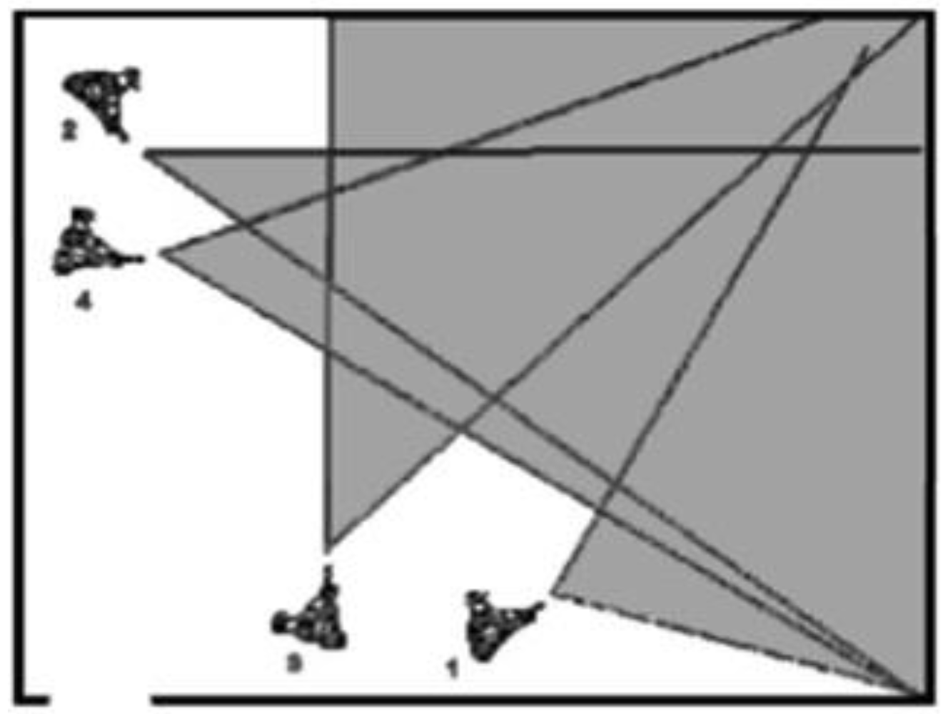
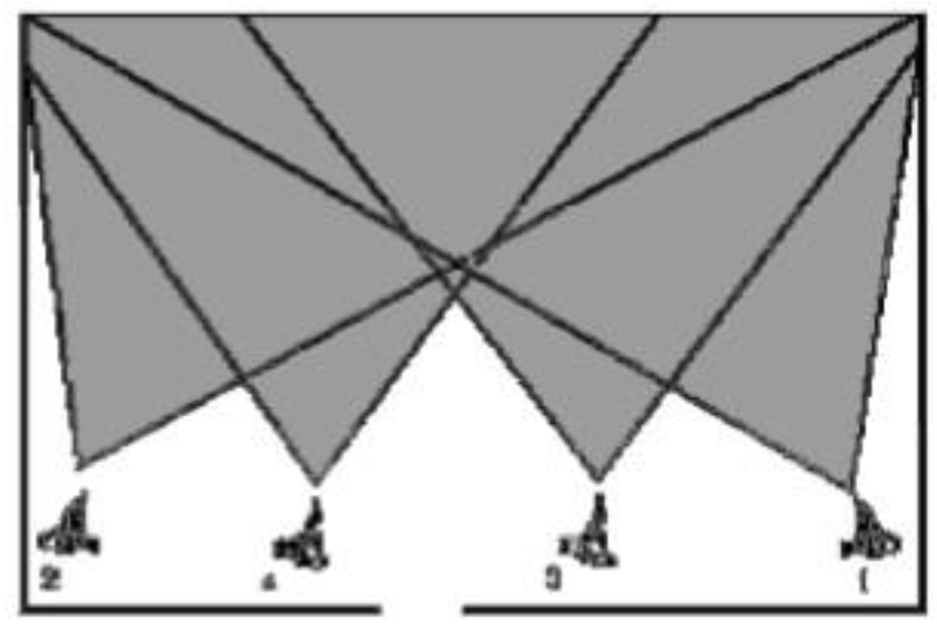
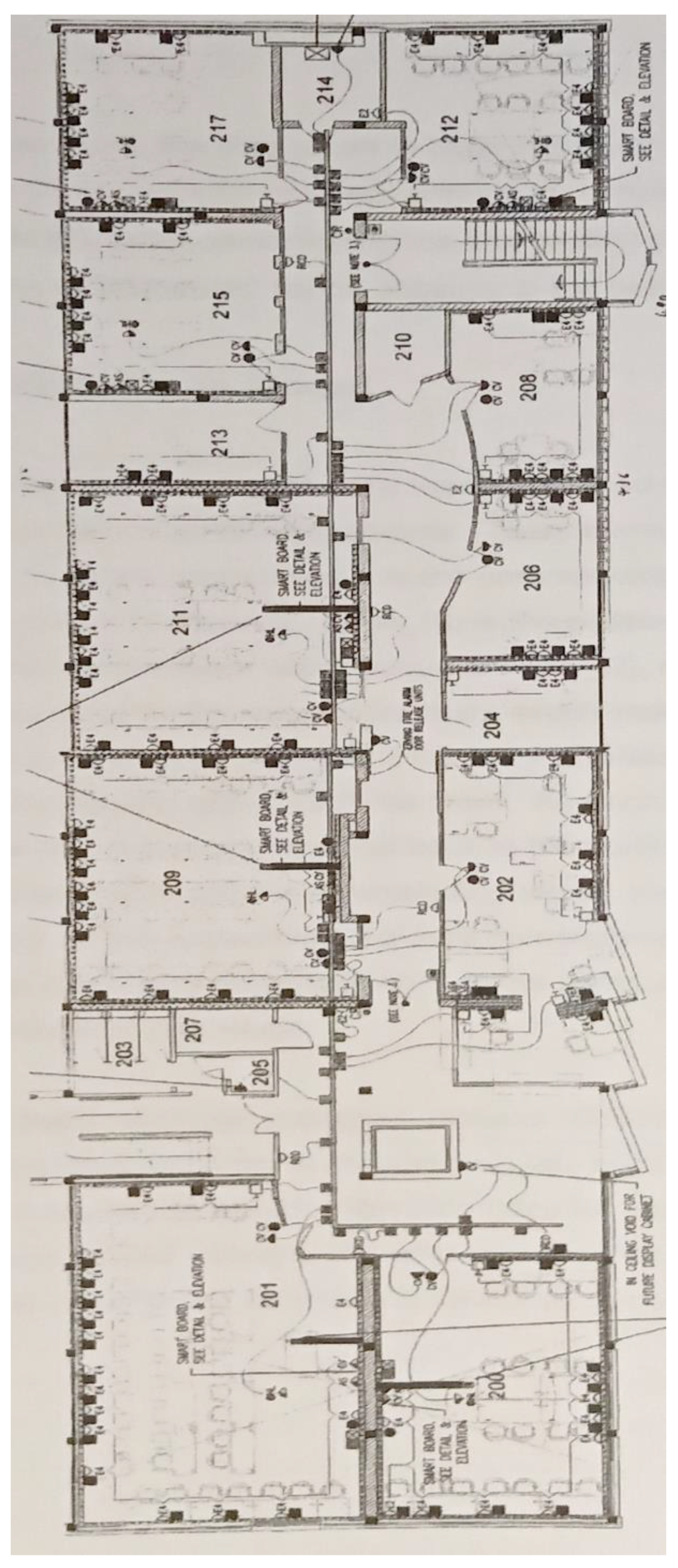
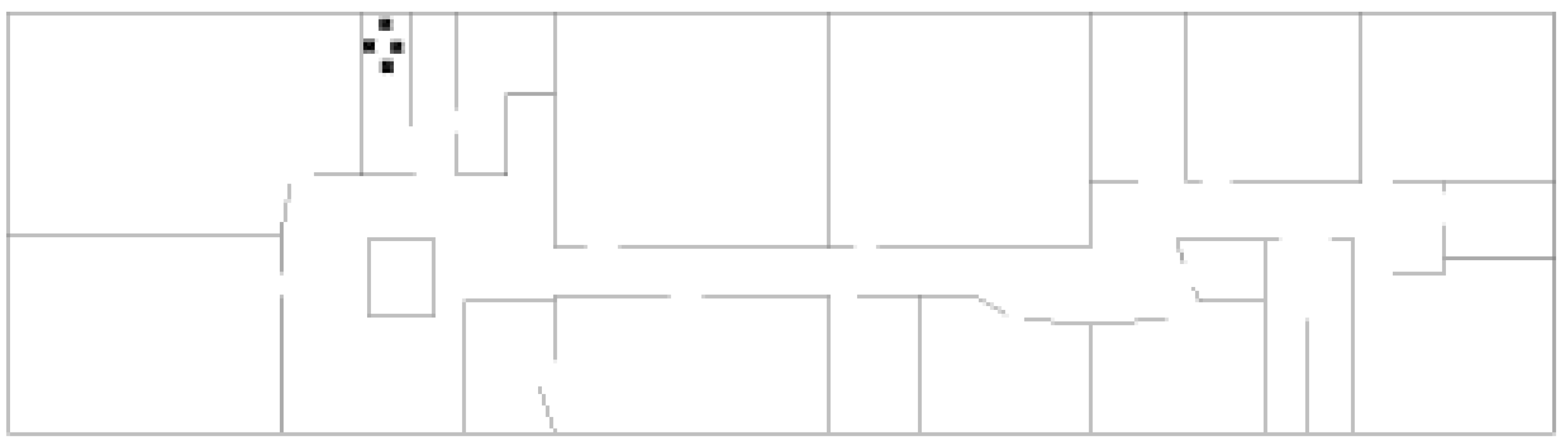
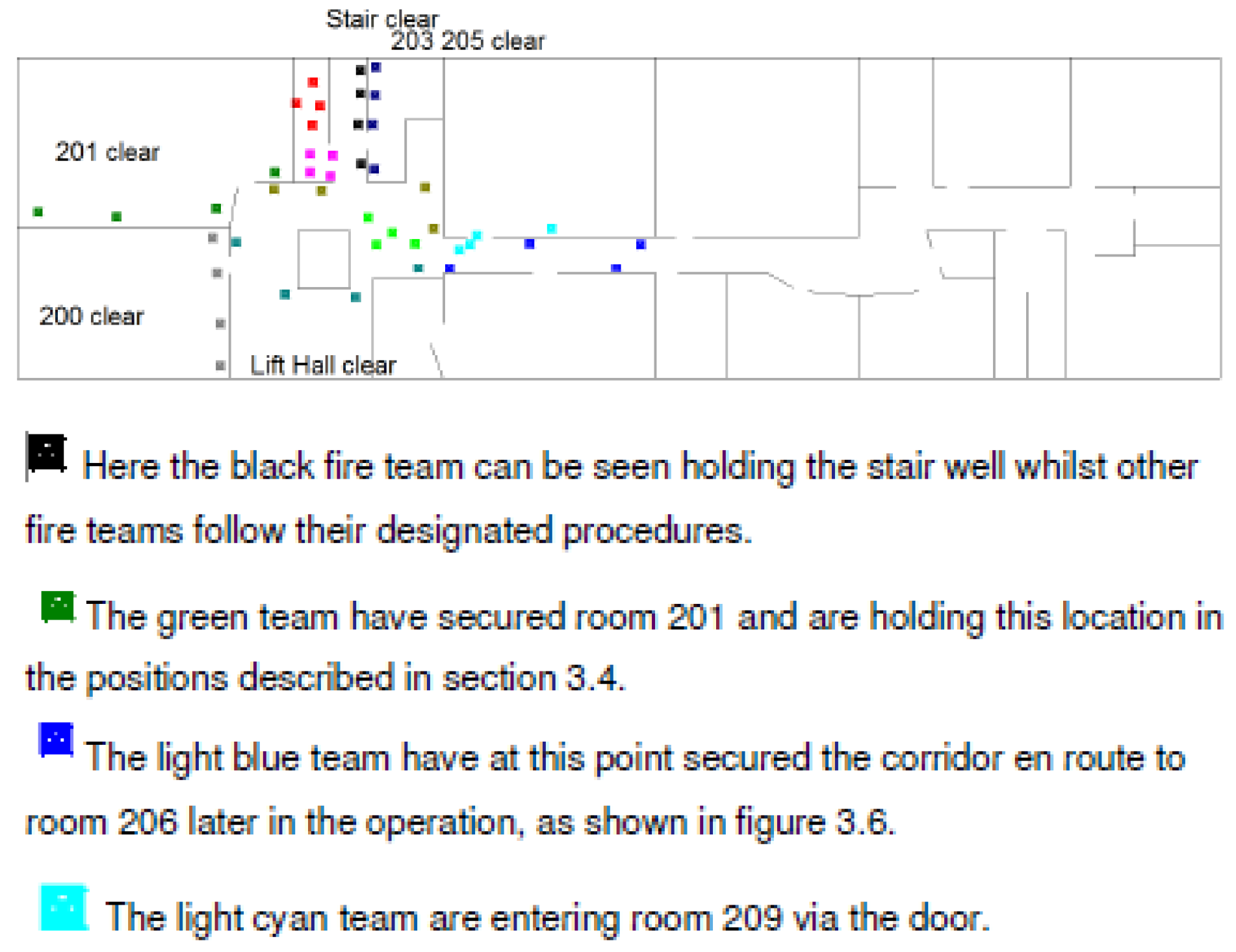
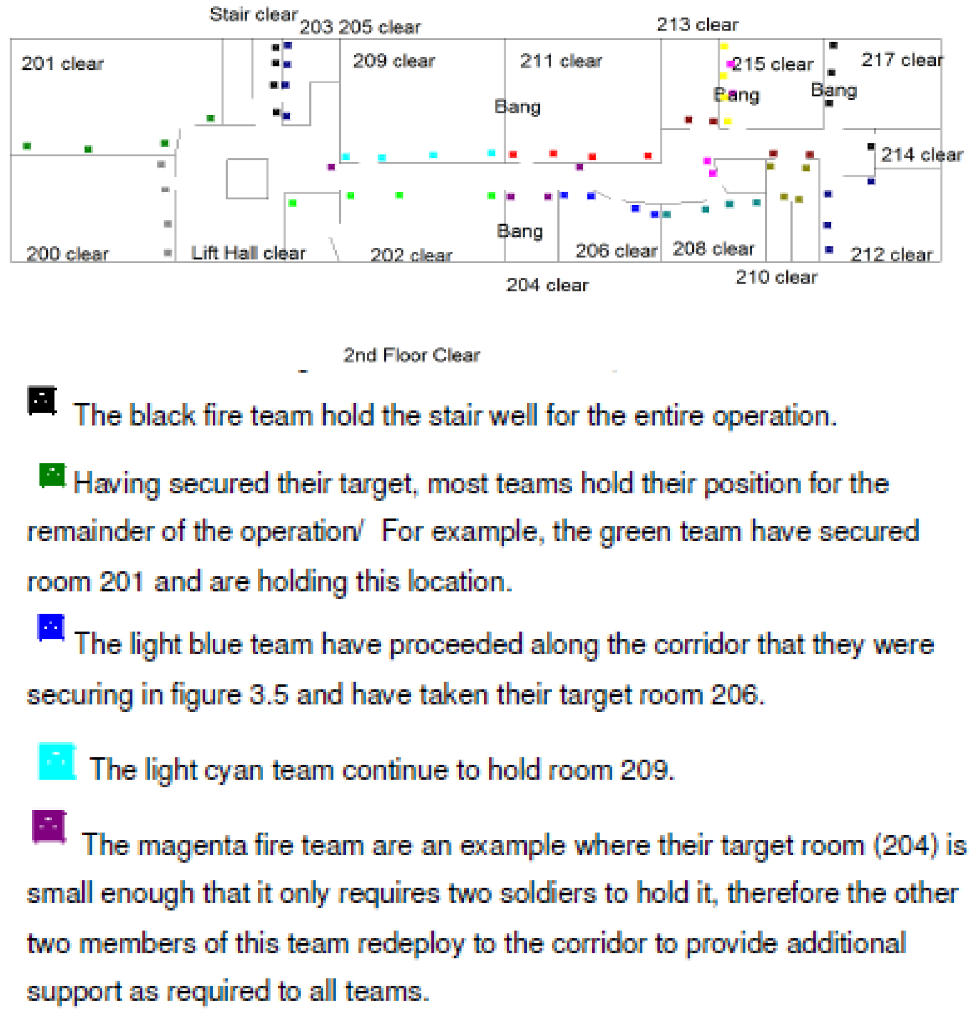
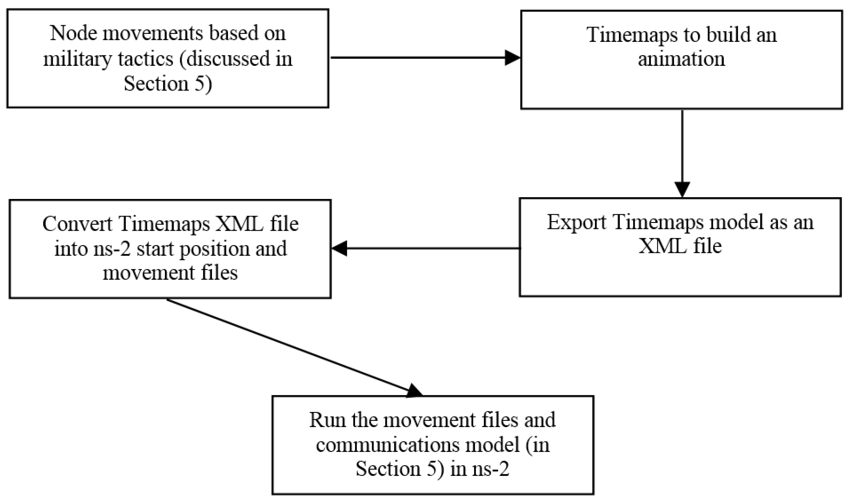
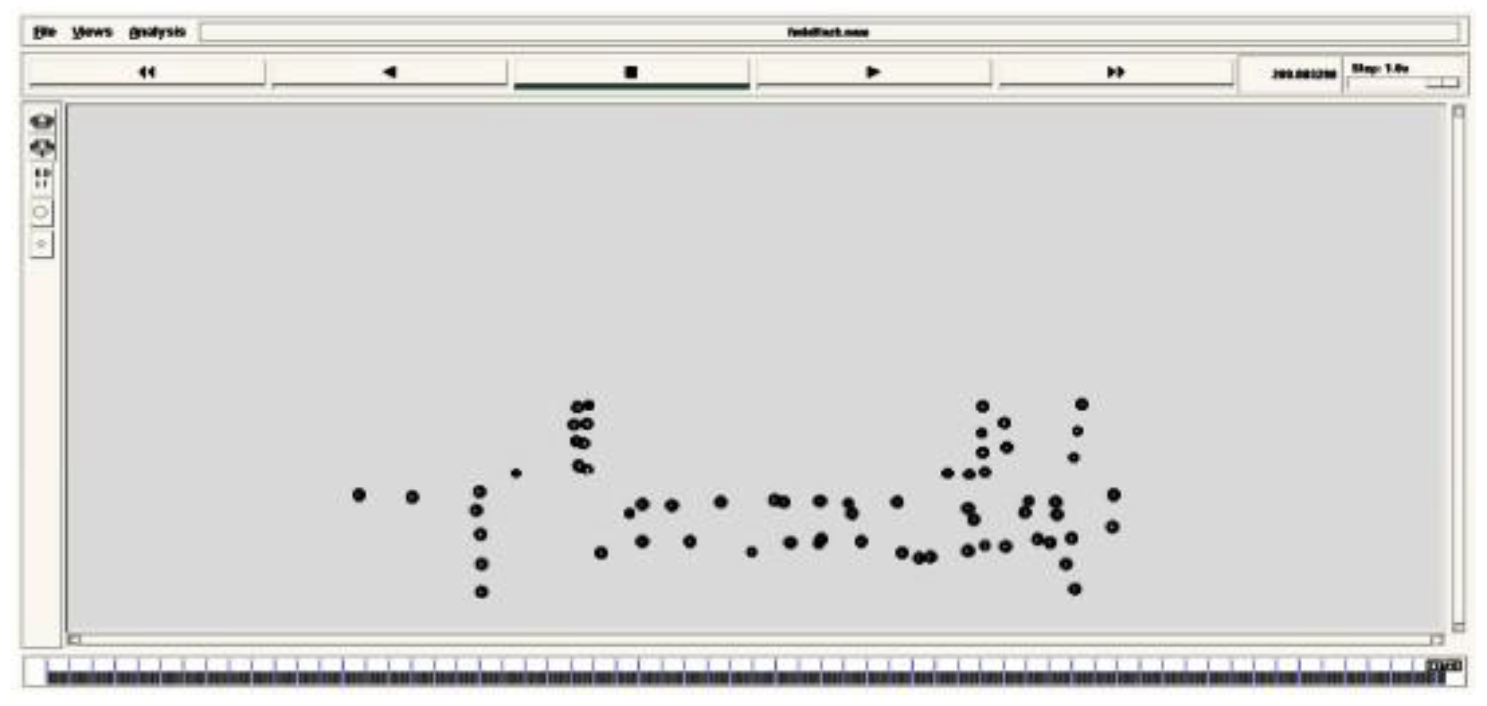
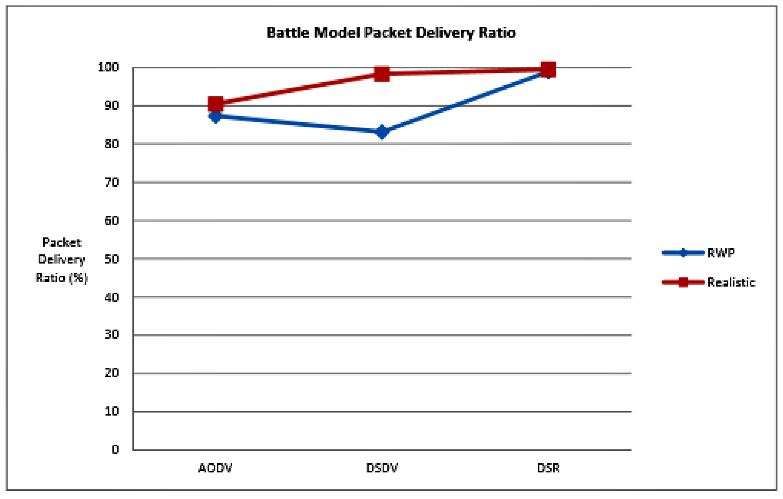
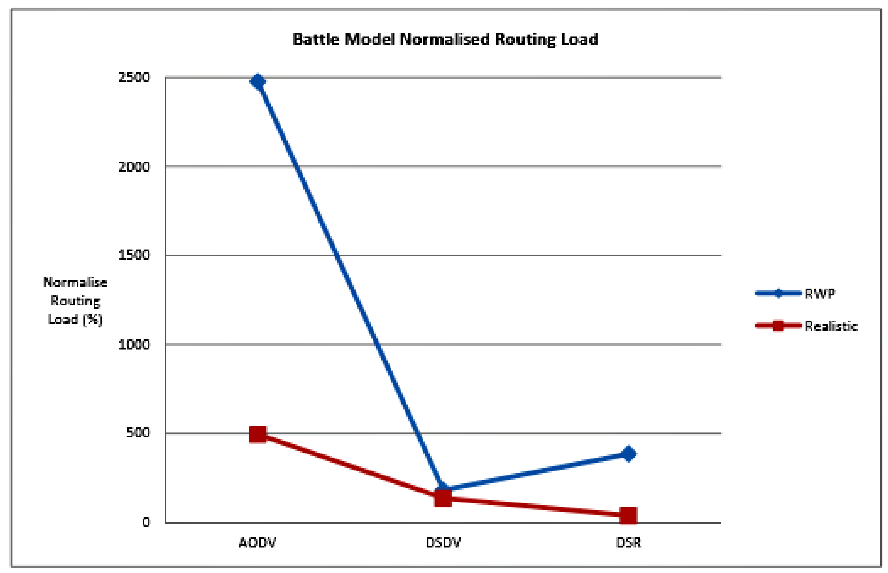
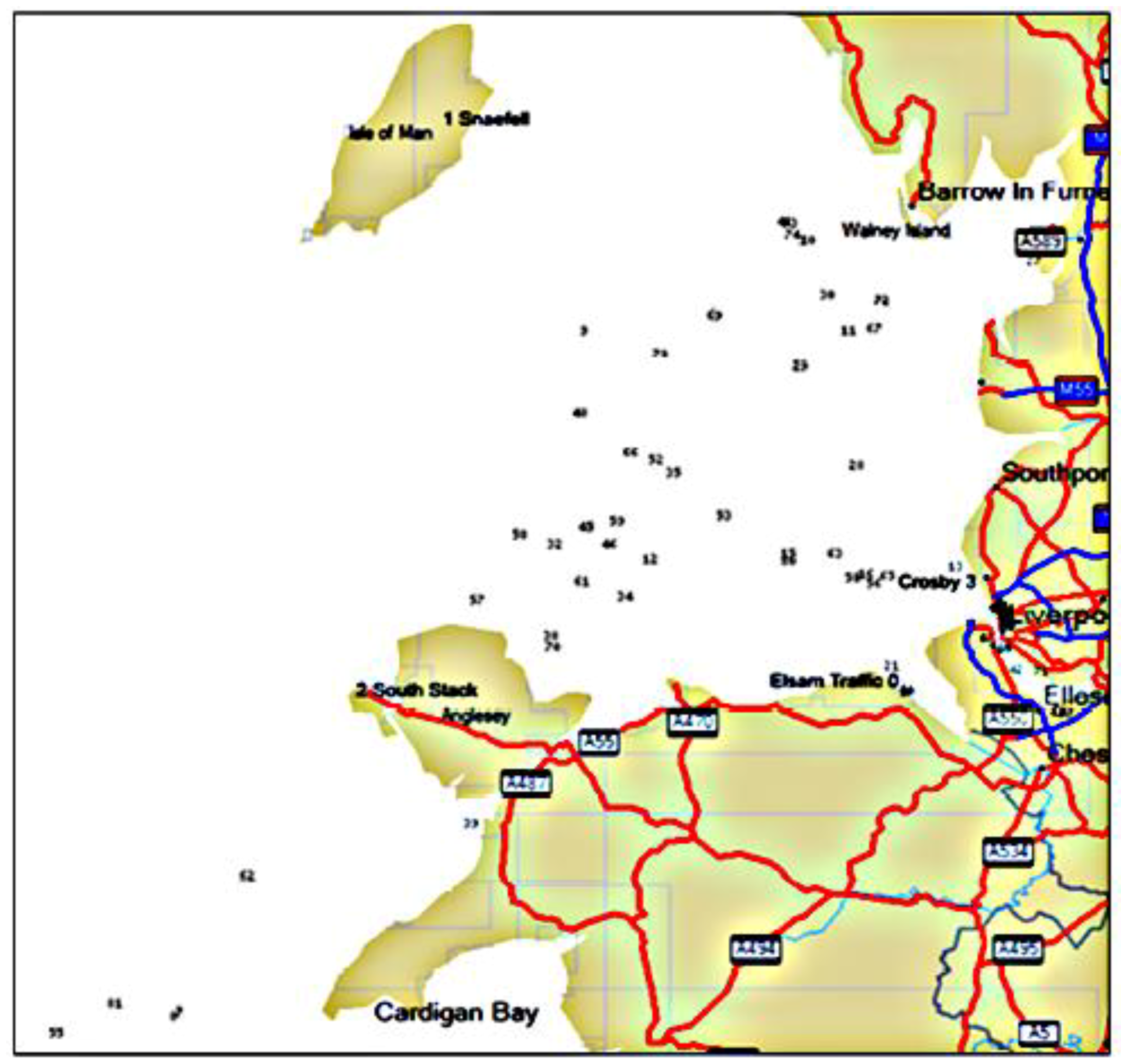
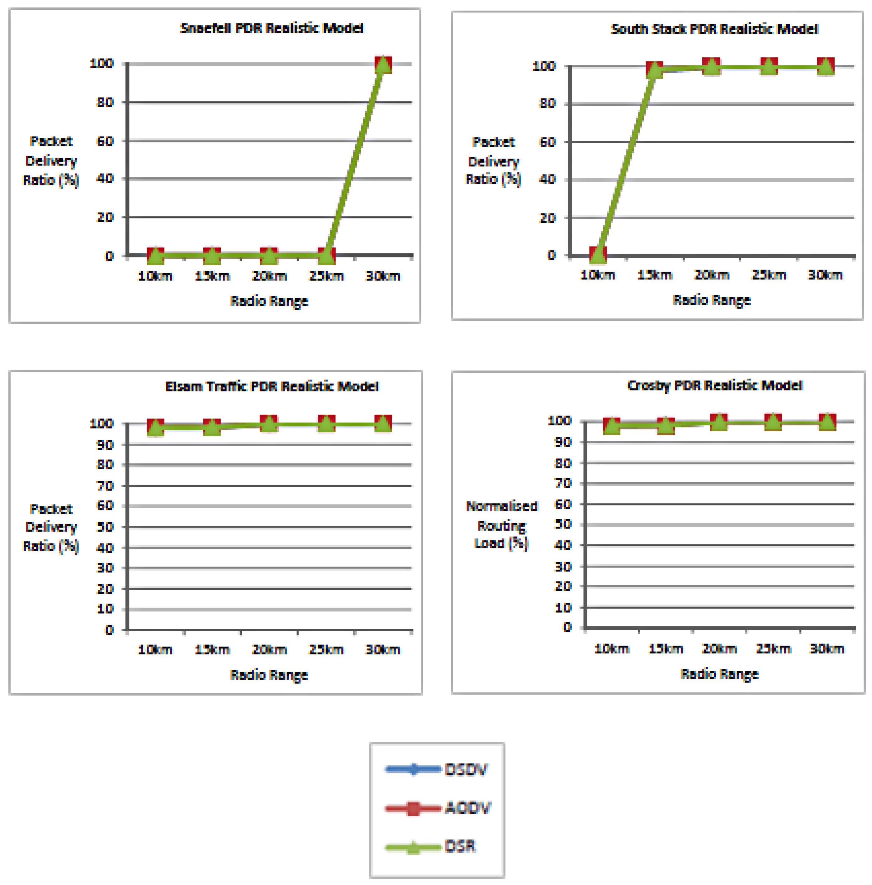
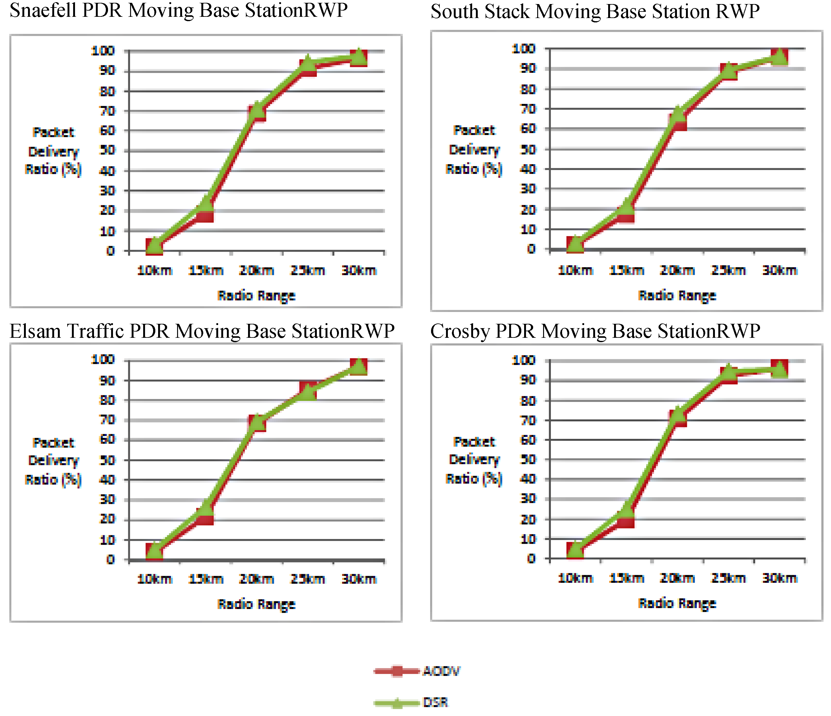
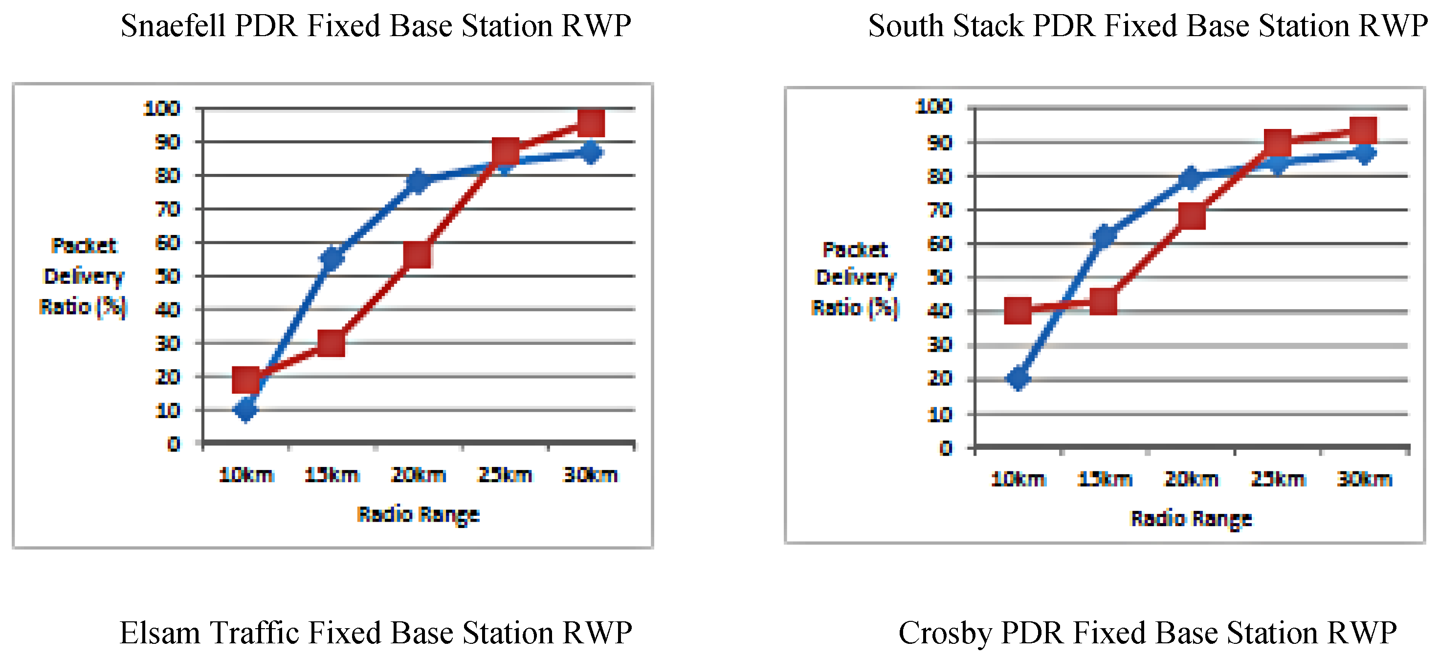
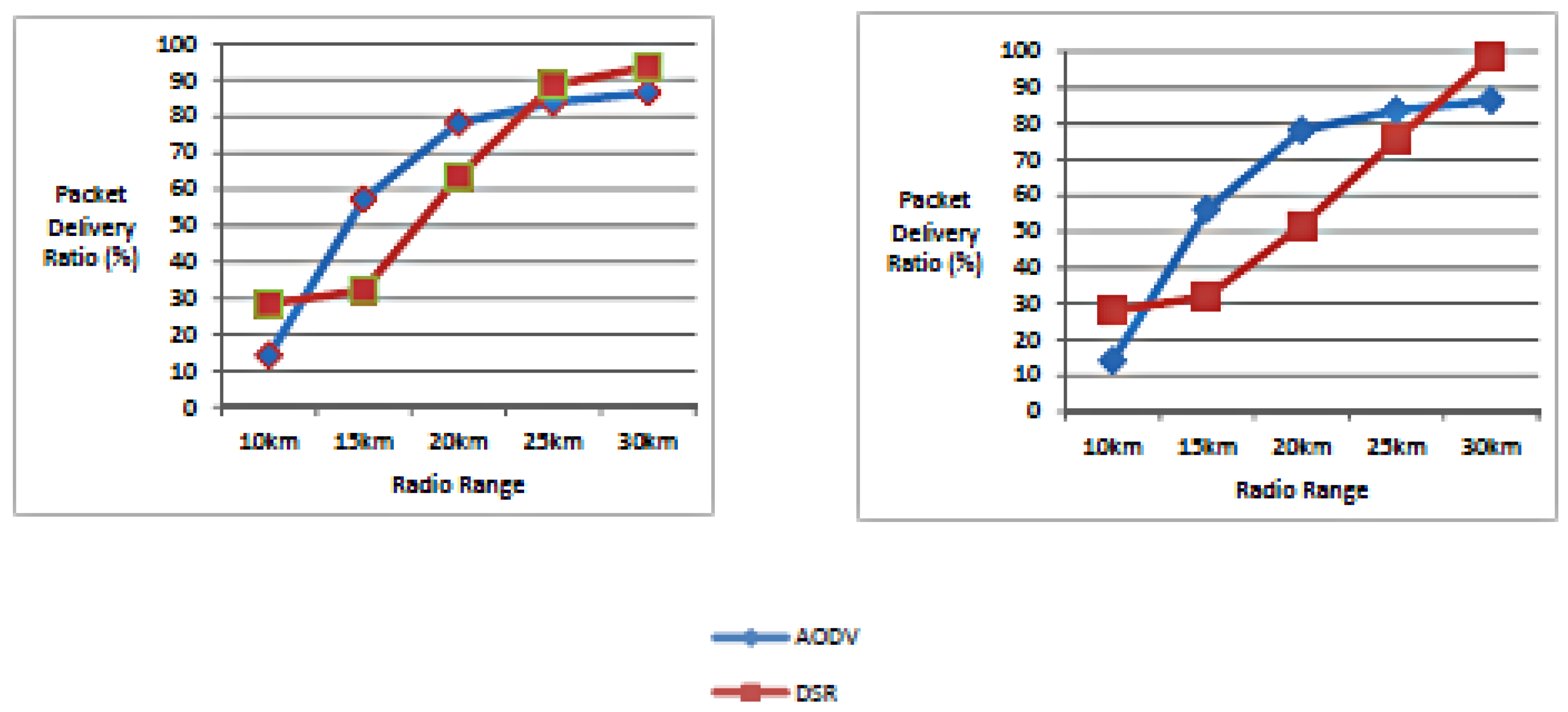
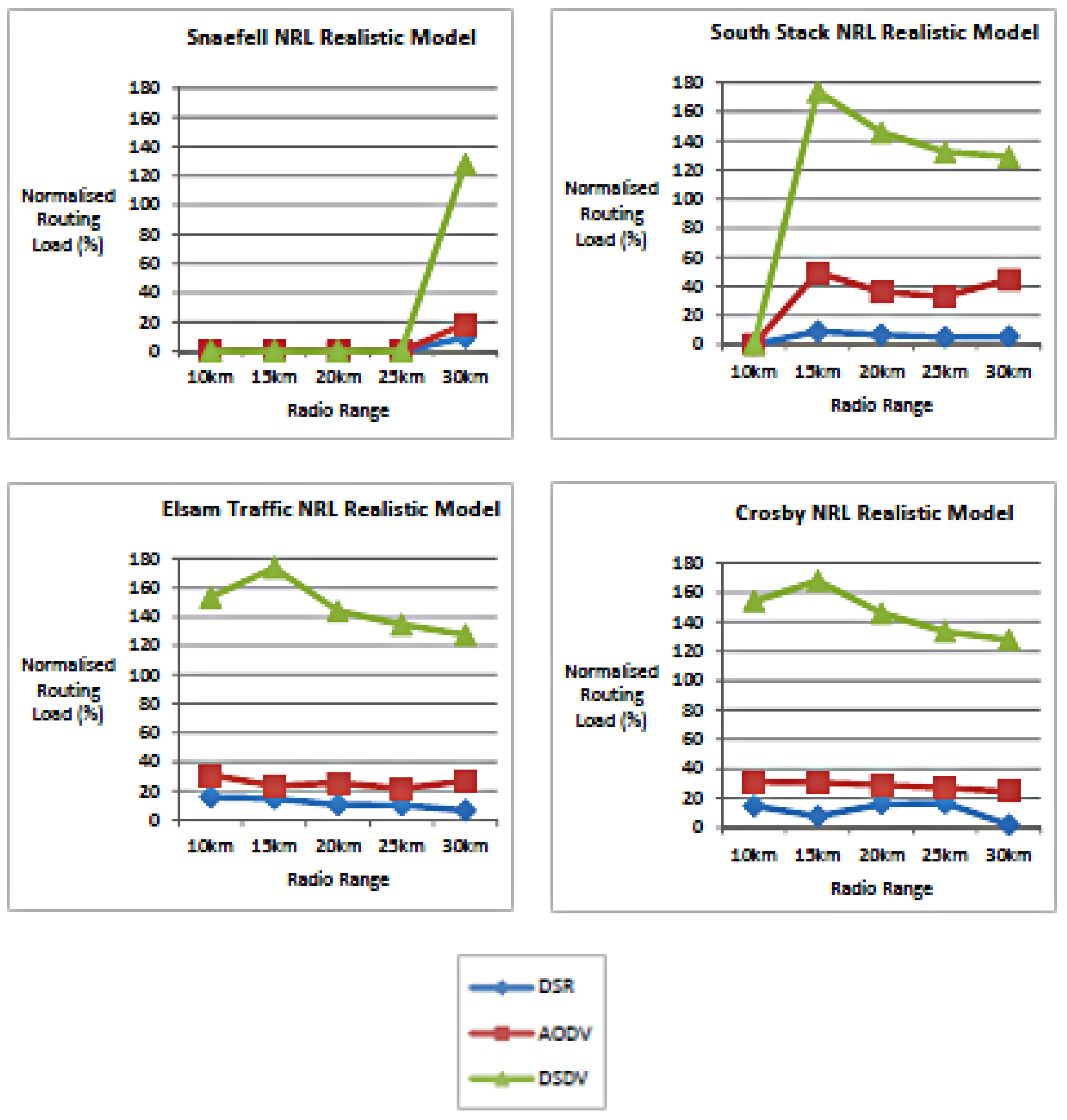
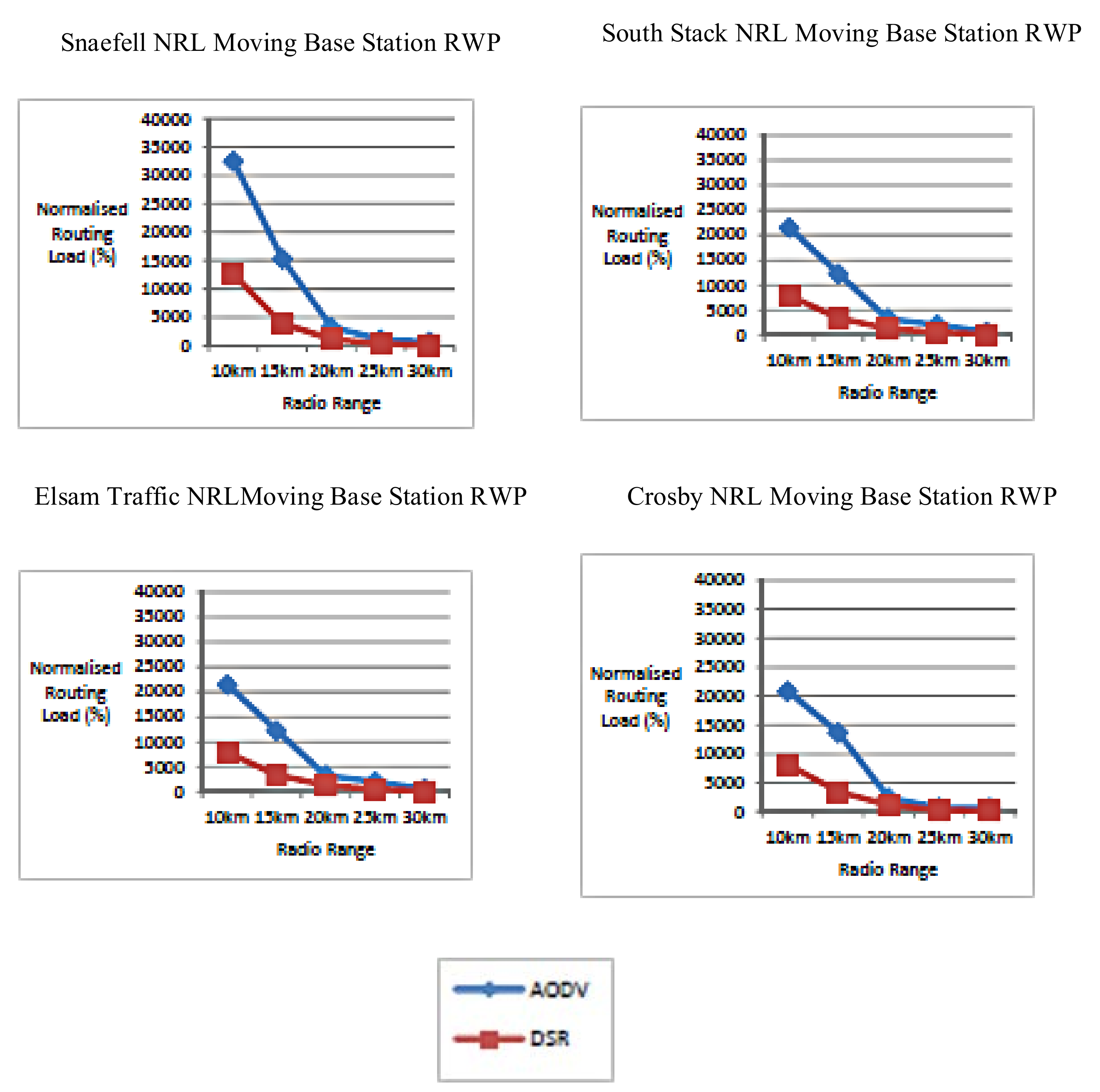
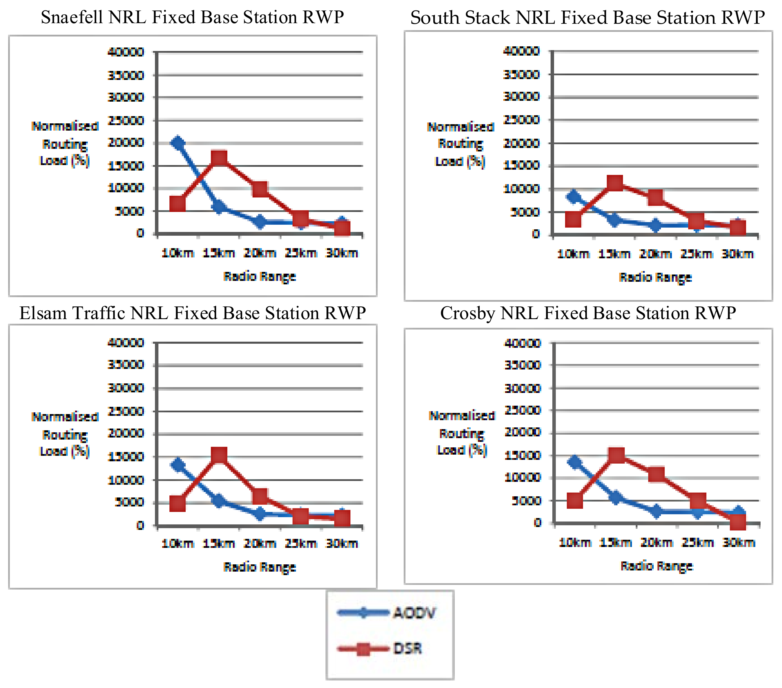
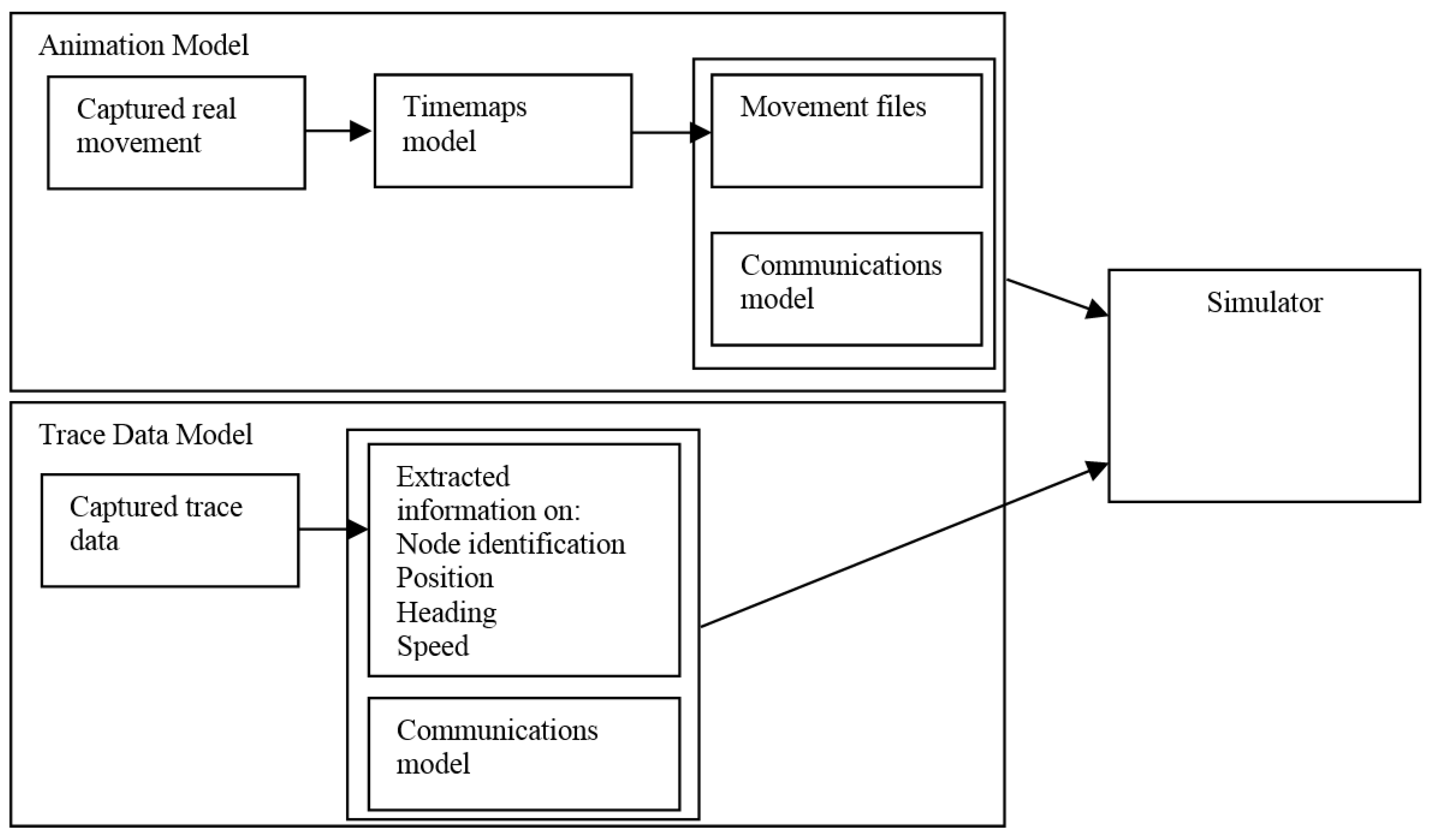
Table 1.
Key Information for a Node.
| Key information for a node is as follows: <class> corps </class> <stringattribute> <name>name</name> <stringtimepoint> <time>2454102.0 15.0 G 2007 1 1 0 0 15</time> <value>$node_(10)</value> </stringtimepoint> </stringattribute> <position> <positiontimepoint> <time>2454102.0 15.0 G 2007 1 1 0 0 15</time> <x> 220.967796</x> <y> 109.528819</y> </positiontimepoint> This translates into a single line in the ns-2 movement file: $ ns_ at 015.000000 “$node_(10) setdest 12.053934 11.875736 0.176657” |
© 2018 by the authors. Licensee MDPI, Basel, Switzerland. This article is an open access article distributed under the terms and conditions of the Creative Commons Attribution (CC BY) license (http://creativecommons.org/licenses/by/4.0/).
Share and Cite
MDPI and ACS Style
Pullin, A.; Pattinson, C.; Kor, A.-L. Building Realistic Mobility Models for Mobile Ad Hoc Networks. Informatics 2018, 5, 22. https://doi.org/10.3390/informatics5020022
AMA Style
Pullin A, Pattinson C, Kor A-L. Building Realistic Mobility Models for Mobile Ad Hoc Networks. Informatics. 2018; 5(2):22. https://doi.org/10.3390/informatics5020022
Chicago/Turabian StylePullin, Adrian, Colin Pattinson, and Ah-Lian Kor. 2018. "Building Realistic Mobility Models for Mobile Ad Hoc Networks" Informatics 5, no. 2: 22. https://doi.org/10.3390/informatics5020022
Note that from the first issue of 2016, this journal uses article numbers instead of page numbers. See further details here.