A Real-Time Optimization Framework for the Iterative Controller Tuning Problem

Abstract

We investigate the general iterative controller tuning (ICT) problem, where the task is to find a set of controller parameters that optimize some user-defined performance metric when the same control task is to be carried out repeatedly. Following a repeatability assumption on the system, we show that the ICT problem may be formulated as a real-time optimization (RTO) problem, thus allowing for the ICT problem to be solved in the RTO framework, which is both very flexible and comes with strong theoretical guarantees. In particular, we propose the use of a recently released RTO solver and outline a simple procedure for how this solver may be configured to solve ICT problems. The effectiveness of the proposed method is illustrated by successfully applying it to four case studies—two experimental and two simulated—that cover the tuning of model-predictive, general fixed-order and PID controllers, as well as a system of controllers working in parallel.

1. Introduction

The typical task of a controller consists in tracking a user-specified trajectory as closely as possible while observing certain additional specifications, such as stability, the satisfaction of safety limits and the minimization of expensive control action when it is not needed. 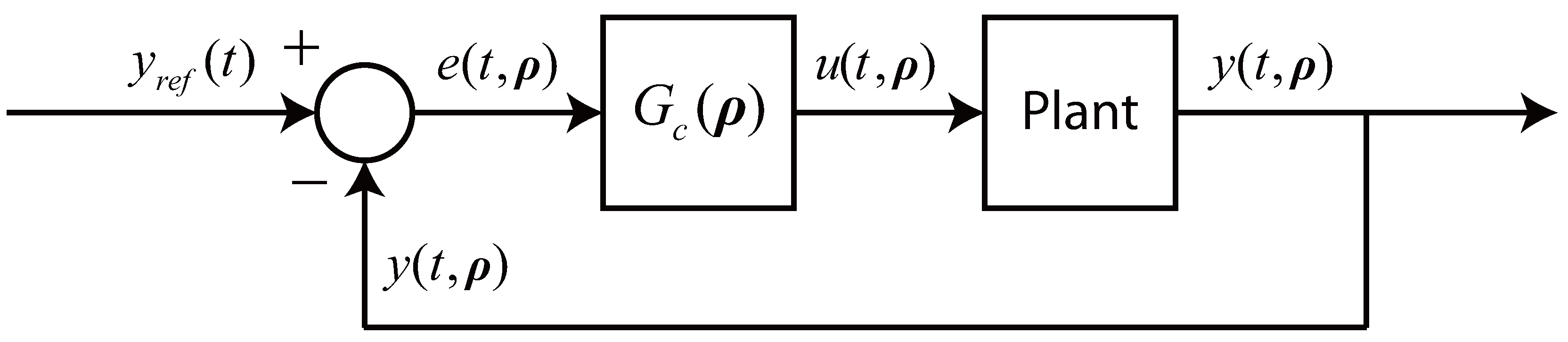Mathematically, we may define such a controller by the mapping $G_c(\mathit{\rho })$, where $\mathit{\rho }\in {\mathbb{R}}^{n_{\rho }}$ denote the parameters that dictate the controller’s behavior and represent decision variables (the “tuning parameters”) for the engineer intending to implement the controller in practice. In the simplest scenario, this often leads to a closed-loop system that may be described by the schematic in Figure 1. No assumptions are made on the nature of $G_c$, which may represent such controllers as the classical PID, the general fixed-order controller, or even the more advanced MPC (model-predictive control). To be even more general, $G_c$ may represent an entire system of such controllers—one would need, in this case, to simply replace $y_{ref}(t)$, $y(t,\mathit{\rho })$, $u(t,\mathit{\rho })$ and $e(t,\mathit{\rho })$ by their vector equivalents.

Figure 1. Qualitative schematic of a single-input-single-output system with the controller $G_c(\mathit{\rho })$. Elements such as disturbances and sensor dynamics, as well as any controller-specific requirements, are left out for simplicity. We use the notation $y(t,\mathit{\rho })$ to mark the (implicit) dependence of the control output on the tuning parameters ρ (likewise for the input and the error).

Figure 1. Qualitative schematic of a single-input-single-output system with the controller $G_c(\mathit{\rho })$. Elements such as disturbances and sensor dynamics, as well as any controller-specific requirements, are left out for simplicity. We use the notation $y(t,\mathit{\rho })$ to mark the (implicit) dependence of the control output on the tuning parameters ρ (likewise for the input and the error).

As with any set of decision variables, it should be clear that there are both good and bad choices of ρ, and in every application, some sort of design phase precedes the actual implementation and acts to choose a set of ρ that is expected to track the reference, $y_{ref}$, “well”, while meeting any additional specifications. The classic example for PID controllers is the Ziegler-Nichols tuning method [1], with methods such as model-based direct synthesis [2] and virtual reference feedback tuning [3] acting as more advanced alternatives. Though not as developed, both theoretical and heuristic approaches exist for the design of MPC [4] and general fixed-order controllers [5,6] as well.

In the majority of cases, the set of controller parameters obtained by these design methods will not be the best possible with respect to control performance. There are many reasons for this, with some of the common ones being:

• assumptions on the plant, such as linearity or time invariance, that are made at the design stage,
• modeling errors and simplifications,
• conservatism in the case of a robust design,
• time constraints and/or deadlines that give preference to a simpler design over an advanced one.

To improve the closed-loop performance of the system, some sort of data-driven adaptation of the parameters from their initial designed values, denoted here by ${\mathit{\rho }}_0$, may be done online following the acquisition of new data. These are generally classified as “indirect” and “direct” adaptations [7] depending on what is actually adapted—the model (followed by a model-based re-design of the controller) in the indirect variant or the controller parameters in the direct one. This paper investigates direct methods that attempt to optimize control performance by establishing a direct link between the observed closed-loop performance and the controller parameters, with the justification that such methods may be forced to converge—at least, theoretically—to a locally optimal choice, ${\mathit{\rho }}^{*}$, regardless of the quality or the availability of the model, which cannot be said for indirect schemes [8].

Many of these schemes attempt to minimize a certain user-defined performance metric (e.g., the tracking error) for a given run or batch by playing with the controller parameters as one would in an iterative optimization scheme—i.e., by changing the parameters between two consecutive runs, trying to discover the effect that this change has on the closed-loop performance (estimating the performance derivatives), and then using the derivative estimates to adapt the parameters further in some gradient-descent manner [9,10,11,12,13]. 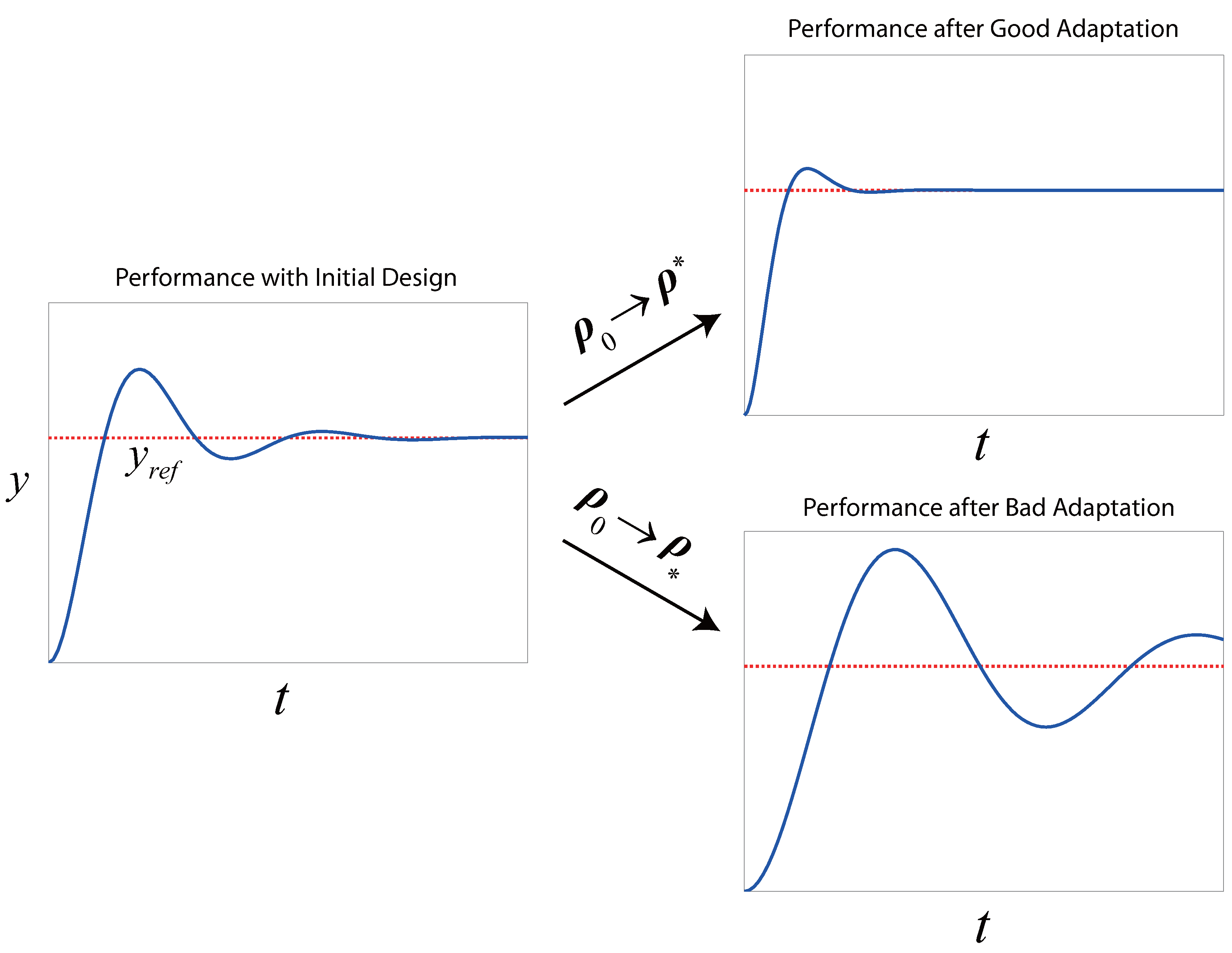This is essentially the iterative controller tuning (ICT) problem, whose goal is to bring the initial suboptimal set, ${\mathit{\rho }}_0$, to the locally optimal ${\mathit{\rho }}^{*}$ via iterative experimentation on the closed-loop system, all the while avoiding that the system become dangerously unstable from the adaptation (a qualitative sketch of this idea is given in Figure 2). A notable limitation of such methods, though rarely stated explicitly, is that the control task for which the controller is being adapted must be identical (or very similar) from one run to the next—otherwise, the concept of optimality may simply not exist, since what is optimal for one control task (e.g., the tracking of a step change) need not be so for another (e.g., the tracking of a ramp). A closely related problem where the assumption of a repeated control task is made formally is that of iterative learning control [14], although what is adapted in that case is the open-loop input trajectory, rather than the parameters of a controller dictating the closed-loop system.

Figure 2. The basic idea of iterative controller tuning. Here, a step change in the setpoint represents the repetitive control task. We use ${\mathit{\rho }}_{*}$ to denote a sort of “anti-optimum” that might be achieved with a bad adaptation algorithm.

Figure 2. The basic idea of iterative controller tuning. Here, a step change in the setpoint represents the repetitive control task. We use ${\mathit{\rho }}_{*}$ to denote a sort of “anti-optimum” that might be achieved with a bad adaptation algorithm.

We observe that, as the essence of these tuning methods consists in iteratively minimizing a performance function that is unknown, due to the lack of knowledge of the plant, the ICT problem is actually a real-time optimization (RTO) problem as it must be solved by iterative experimentation. Recent work by the authors [15,16,17] has attempted to unify different RTO approaches and to standardize the RTO problem as any problem having the following canonical form:

$$\begin{array}{cc}\hfill \underset{\mathbf{v}}{\mathrm{minimize}}& {\varphi }_p(\mathbf{v})\hfill \\ \hfill \mathrm{subject}\mathrm{to}& {\mathbf{G}}_p(\mathbf{v})⪯\mathbf{0}\hfill \\ & \mathbf{G}(\mathbf{v})⪯\mathbf{0}\hfill \\ & {\mathbf{v}}^L⪯\mathbf{v}⪯{\mathbf{v}}^U\hfill \end{array}$$

(1)

where $\mathbf{v}\in {\mathbb{R}}^{n_v}$ denote the RTO variables (RTO inputs) forced to lie in the relevant RTO input space defined by the lower and upper limits, ${\mathbf{v}}^L$ and ${\mathbf{v}}^U$, ${\varphi }_p$ denotes the cost function to be minimized, and ${\mathbf{G}}_p$ and $\mathbf{G}$ denote the sets of individual constraints, $g_p,g:{\mathbb{R}}^{n_v}\to \mathbb{R}$ (i.e., safety limitations, performance specifications), to be respected. We use the symbol ⪯ to denote componentwise inequality.

The subscript p (for “plant”) is used to indicate those functions that are unknown, or “uncertain”, and can only be evaluated by applying a particular ${\mathbf{v}}_k$ and conducting a single experiment (with k denoting the experiment/iteration counter), from which the corresponding function values may then be measured or estimated:

$$\begin{array}{c}{\widehat{\varphi }}_p({\mathbf{v}}_k)={\varphi }_p({\mathbf{v}}_k)+w_{\varphi ,k}\hfill \\ {\widehat{g}}_p({\mathbf{v}}_k)=g_p({\mathbf{v}}_k)+w_{g,k}\hfill \end{array}$$

(2)

with some additive stochastic error, w. Conversely, the absence of p indicates that the function is easily evaluated by algebraic calculation without any error present.

Owing to the generality of Problem (1), casting the ICT problem in this form is fairly straightforward and, as will be shown in this work, has numerous advantages, as it allows for a fairly systematic and flexible approach to controller tuning in a framework where strong theoretical guarantees are available. The main contribution of our work is thus to make this generalization formally and to argue for its advantages, while cautioning the potential user of both its apparent and hypothetical pitfalls.

Our second contribution lies in proposing a concrete method for solving the ICT problem in this manner. Namely, we advocate the use of the recently released open-source SCFO (“sufficient conditions for feasibility and optimality”) solver that has been designed for solving RTO problems with strong theoretical guarantees [17]. While this choice is undoubtedly biased, we put it forward as it is, to the best of our knowledge, the only solver released to date that solves the RTO problem (1) reliably, which is to say that it consistently converges to a local minimum without violating the safety constraints in theoretical settings and that it is fairly robust in doing the same in practical ones. Though quite simple to apply, the SCFO framework and the solver itself need to be properly configured, and so we guide the potential user through how to configure the solver for the ICT problem.

Finally, as the theoretical discussion alone should not be sufficient to convince the reader that there is a strong potential for solving the ICT problem as an RTO one, we finish the paper with a total of four case studies, which are intended to cover a diverse range of experimental and simulated problems and to demonstrate the general effectiveness of the proposed method, the difficulties that are likely to be encountered in application, and any weak points where the methodology still needs to be improved. Specifically, the four studies considered all solve the ICT problem for:

• the tracking of a temperature profile in a laboratory-scale stirred tank by an MPC controller,
• the tracking of a periodic setpoint for a laboratory-scale torsional system by a general fixed-order controller with a controller stability constraint,
• the PID tracking of a setpoint change for various linear systems (previously examined in [13,18]),
• the setpoint tracking and disturbance rejection for a five-input, five-output multi-loop PI system with imperfect decoupling and a hard output constraint.

In each case, we do our best to concretize the theory discussed earlier by showing how the resulting ICT problem may be formulated in the RTO framework, followed by the application of the SCFO solver with the proposed configuration.

2. The RTO Formulation of the Iterative Controller Tuning Problem

In this section, we go through the different components of the RTO problem (1) and state their ICT analogues, together with any assumptions necessary to make the links between the two clean. We then finish by reviewing the benefits and limitations of this approach.

2.1. The Cost Function ${\varphi }_p$ → The Control Performance Metric

The intrinsic driving force behind iteratively tuning a controller so that it performs “better” is the somewhat natural belief that there is some sort of deterministic link between the parameters and the observed performance. We qualify this via the following assumption, which was originally stated in the MPC context in [19] and then extended to the general controller in [20].

Assumption 1 (Repeatability). Let $\mathit{\rho }\in {\mathbb{R}}^{n_{\rho }}$ denote the tuning parameters of a controller and $J_k$ the observed value of the user-defined performance metric at run k for a fixed control task that is identical from run to run. The closed-loop process is repeatable with respect to performance if:

$$J_k=J({\mathit{\rho }}_k)+{\delta }_k$$

(3)

where ${\mathit{\rho }}_k$ are the parameters of the controller at run k, $J:{\mathbb{R}}^{n_{\rho }}\to \mathbb{R}$ is a purely deterministic relation between the performance metric and the parameters, and ${\delta }_k$ is the “non-repeatability noise”, a purely stochastic element that is independent of ${\mathit{\rho }}_k$.

In layman’s terms, the (unknown) function, J, is precisely the intrinsic link that we believe in, while ${\delta }_k$ is a representation of reality, which most often manifests itself by means of measurement noise and differs unpredictably from run to run. The discussion of the validity of such an assumption is deferred to the end of the section.

Comparing (2) and (3), both of which involve a deterministic function that is sampled with additive noise, we establish our first RTO → ICT connection:

$$\underset{\mathbf{v}}{\mathrm{minimize}}{\varphi }_p(\mathbf{v})\to \underset{\mathit{\rho }}{\mathrm{minimize}}J(\mathit{\rho })$$

(4)

A common general performance metric, given here in continuous form for the single-input-single-output (SISO) case, may be defined as:

$${\displaystyle J_k:={\lambda }_1{\int }_0^{t_b}{\left[y_{ref}(t)-y(t,{\mathit{\rho }}_k)\right]}^{2}dt+{\lambda }_2{\int }_0^{t_b}{u}^2(t,{\mathit{\rho }}_k)dt+{\lambda }_3{\int }_0^{t_b}{\dot{y}}^2(t,{\mathit{\rho }}_k)dt+{\lambda }_4{\int }_0^{t_b}{\dot{u}}^2(t,{\mathit{\rho }}_k)dt}$$

(5)

where $t_b$ denotes the total length of a single run and where the weights, $\mathit{\lambda }⪰\mathbf{0}$, may be set as needed to trade off between giving preference to tracking error, the control action, the smoothness of the output response, and the aggressiveness of the controller. Modifications that include other criteria, such as frequency weighting [10], or that modify the time interval for which the performance is analyzed by adding a “mask” [18], are of course possible as well.

2.2. The Uncertain Inequality Constraints ${\mathbf{G}}_p$ → Safety and Economic Constraints

Many control applications may have strict safety specifications that require a given output, $y(t,\mathit{\rho })$, to remain within a certain zone, defined by $\underline{y}$ and $\overline{y}$, throughout the length of the run:

$$\underline{y}\le y(t,\mathit{\rho })\le \overline{y},\forall t\in [0,t_b]$$

(6)

While it is not difficult to propose methods to enforce such behavior for the general controller, many of which would likely try to incorporate the constraints as setpoint objectives, such approaches remain largely ad hoc. This drawback has shifted particular emphasis to MPC as being the advanced controller to be able to deal with output constraints systematically [21], but even here no rigorous conditions for satisfying (6) are available for the general case where any amount of plant-model mismatch is admissible.

Since rigorous theoretical conditions are available for satisfying ${\mathbf{G}}_p(\mathbf{v})⪯\mathbf{0}$ in the RTO framework [15], we may exploit this advantage by casting the hard output constraints for the ICT problem in RTO form. To do this, we start by replacing the two semi-infinite constraints of Equation (6) by their equivalent finite versions:

$$\begin{array}{c}\underline{y}\le \underset{t\in [0,t_b]}{min}y(t,\mathit{\rho })\hfill \\ \underset{t\in [0,t_b]}{max}y(t,\mathit{\rho })\le \overline{y}\hfill \end{array}$$

At this point, we need to apply a version of Assumption 1 for the constraints. For a particular run, k, we assume that the closed-loop process is repeatable with respect to the control output range:

$$\begin{array}{c}\underset{t\in [0,t_b]}{min}y(t,{\mathit{\rho }}_k)=y_{min}({\mathit{\rho }}_k)+{\delta }_{min,k}\hfill \\ \underset{t\in [0,t_b]}{max}y(t,{\mathit{\rho }}_k)=y_{max}({\mathit{\rho }}_k)+{\delta }_{max,k}\hfill \end{array},$$

(7)

i.e., that the minimum and maximum values of the trajectory $y(t,{\mathit{\rho }}_k)$ observed for a given run k are (unknown) deterministic functions ($y_{min}$, $y_{max}$) of the parameters plus a stochastic element (${\delta }_{min,k}$, ${\delta }_{max,k}$).

Making the link with Equation (2), we may now restate the hard output constraints in RTO form as:

$${\mathbf{G}}_p(\mathbf{v})⪯\mathbf{0}\to \begin{array}{c}-y_{min}(\mathit{\rho })+\underline{y}\le 0\hfill \\ y_{max}(\mathit{\rho })-\overline{y}\le 0\hfill \end{array}$$

(8)

where the function values $y_{min}$ and $y_{max}$ can be measured for a given ρ with the additive errors ${\delta }_{min}$ and ${\delta }_{max}$.

Alternatively, it may occur that there are economic constraints with respect to the inputs. As an example, consider a reactor where one of the control inputs is the feed rate of a reagent. While effective for the purposes of control, the reagent may be expensive and so only a limited amount may be allotted per batch, with the constraint:

$${\displaystyle {\int }_0^{t_b}u(t,\mathit{\rho })dt\le {\overline{u}}_T}$$

imposed, where ${\overline{u}}_T$ is some user-defined limit. Following the same steps as above, we suppose that:

$${\displaystyle {\int }_0^{t_b}u(t,{\mathit{\rho }}_k)dt=u_T({\mathit{\rho }}_k)+{\delta }_{u,k}}$$

with $u_T$ the deterministic component and ${\delta }_u$ the non-repeatability noise, and make the connection:

$${\mathbf{G}}_p(\mathbf{v})⪯\mathbf{0}\to u_T(\mathit{\rho })-{\overline{u}}_T\le 0$$

It should be clear that extension to multiple-input-multiple-output (MIMO) cases is trivial, as this only adds more elements to ${\mathbf{G}}_p$.

2.3. The Certain Inequality Constraints $\mathbf{G}$ → Controller Specifications and Stability Considerations

In some controllers, analytically known inequality relations may need to be satisfied. One such example is the case of the MPC controller, where one may tune both the control and prediction horizons (m and n, respectively) with the built-in rule [21]:

$$m\le n$$

(9)

which, if we define ${\rho }_1\stackrel{\Delta }{=}m$ and ${\rho }_2\stackrel{\Delta }{=}n$, leads to the following link with Equation (1):

$$\mathbf{G}(\mathbf{v})⪯\mathbf{0}\to {\rho }_1-{\rho }_2\le 0$$

As another example, we may want to adapt the parameters of the discrete fixed-order controller:

$${\displaystyle G_c(\mathit{\rho })=\frac{{\rho }_1{z}^2+{\rho }_{2}z+{\rho }_3}{z^2+{\rho }_{4}z+{\rho }_5}}$$

(10)

but would like to limit our search to stable controllers only. Employing the Jury stability criterion [22], we generate the first four rows of the Jury table for the denominator of $G_c(\mathit{\rho })$:

$$\begin{array}{cccc}\mathrm{row}1:\hfill & 1& {\rho }_4& {\rho }_5\\ \mathrm{row}2:\hfill & {\rho }_5& {\rho }_4& 1\\ \mathrm{row}3:\hfill & 1-{\rho }_5^2& {\rho }_4-{\rho }_4{\rho }_5& 0\\ \mathrm{row}4:\hfill & {\rho }_4-{\rho }_4{\rho }_5& 1-{\rho }_5^2& 0\end{array}$$

from which the sufficient conditions for controller stability are obtained as:

$$\begin{array}{c}|{\rho }_5|<1\hfill \\ |{\rho }_4-{\rho }_4{\rho }_5|<|1-{\rho }_5^2|\hfill \end{array}\to \begin{array}{c}|{\rho }_5|\le 1-\epsilon \hfill \\ |{\rho }_4-{\rho }_4{\rho }_5|\le |1-{\rho }_5^2|-\epsilon \hfill \end{array}$$

(11)

with the constraint set on the right representing an implementable non-strict version with negligible conservatism for $\epsilon >0$ small. Controller stability may now be ensured in the RTO form with the correspondence:

$$\mathbf{G}(\mathbf{v})⪯\mathbf{0}\to \begin{array}{c}|{\rho }_5|-1+\epsilon \le 0\hfill \\ |{\rho }_4-{\rho }_4{\rho }_5|-|1-{\rho }_5^2|+\epsilon \le 0\hfill \end{array}$$

(12)

Finally, we note that nominal closed-loop stability constraints may also be incorporated in this manner. As a simple example, consider the unstable plant that is modeled as:

$$G(s)=\frac{1}{s-1}$$

and that is to be controlled by a PD controller with ${\rho }_1$ and ${\rho }_2$ the proportional and derivative gains, respectively:

$$G_c(\mathit{\rho })={\rho }_1+{\rho }_{2}s$$

From the analysis of the characteristic equation, $1+G{G}_c=0$, we have the stability condition, together with its implementable version:

$$\frac{1-{\rho }_1}{1+{\rho }_2}<0\to \frac{1-{\rho }_1}{1+{\rho }_2}\le -\epsilon$$

which, again, allows the correspondence:

$$\mathbf{G}(\mathbf{v})⪯\mathbf{0}\to \frac{1-{\rho }_1}{1+{\rho }_2}+\epsilon \le 0$$

(13)

Extensions to robust nominal stability follow easily and would simply involve a greater number of constraints.

2.4. The Box Constraints ${\mathbf{v}}^L⪯\mathbf{v}⪯{\mathbf{v}}^U$ → Controller Parameter Limits

Given the RTO-ICT correspondence of $\mathbf{v}\to \mathit{\rho }$, the box constraints of the RTO problem are simply the lower and upper limits, ${\mathit{\rho }}^L$ and ${\mathit{\rho }}^U$, on the adapted controller parameters. We note that certain limits will be obvious for certain controllers—e.g., the integral time should be superior to zero in a PI controller, while the prediction and control horizons of an MPC controller should be equal to or greater than one. In other cases, one may have to think a little before deciding on appropriate limits. In Section 3, an easy way to set parameter bounds for the general controller will be provided.

2.5. The ICT Problem in RTO Form: Summary

Having now gone through all the components of Problem (1) and having provided their ICT analogues, we may make certain remarks and observations.

To start with the positive, almost all of the possible desired specifications in a standard ICT problem are easily stated in RTO terms, although this is not surprising, given the generality of the formulation (1). Of particular interest with regard to this point are the constraint terms, as the flexibility of the RTO formulation has allowed for us to include limits on the control outputs and inputs, as well as any controller specifications, very easily. To the best of the authors’ knowledge, constraints are generally avoided in the majority (though not all [23]) of direct tuning formulations. This is likely because the most commonly used method—the gradient descent—is not well-equipped to deal with them (apart from certain simple kinds, such as the box constraints [19]). Casting the ICT problem in the RTO framework therefore allows us to ignore this limitation.

The other big advantage is that no assumptions are needed on the nature of the controller (or their number, if a system of controllers is considered)—it simply has to be something that can be parametrically tuned, and so one could adapt just about anything. Likewise, the standard restricting assumption of linearity is also not needed, even formally, as the black-box nature of the RTO formulation does not make use of such assumptions since it ignores the actual dynamic behavior of the closed loop and only considers the RTO inputs (the tuning parameters) and RTO outputs (performance, proximity to constraints), both of which are static quantities with a static map between them. As such, the methodology applies just as readily to nonlinear systems as it does to linear ones.

There are, however, points to be contested. The key linking element between RTO and ICT is Assumption 1, which is, at best, only an approximation and merits justification. The driving force behind this assumption is the fact that any deterministic controller with fixed tuning parameters, when applied repeatedly to a closed-loop process to perform the same control task, should always yield the exact same performance (and the exact same input/output trajectories) in the absence of non-repeatable effects such as input/measurement noise, process degradation and disturbances. Indeed, the absence of such effects implies that the ${\delta }_k$ term in Equation (3) is equal to zero and that the repeatability assumption holds exactly. For cases when these effects are minor and do not influence controller behavior significantly, we expect that a given controller will yield the same performance “more or less”, with variations being lumped into ${\delta }_k$ and the major deterministic trends being described by J. This neat way of decoupling the deterministic and stochastic components may not be valid when the non-repeatable effects become large and exert a significant influence on the controller behavior, however. As such, we may view this assumption as an approximation of reality that tends to perfection as the magnitude of the noise/degradation/disturbances in the closed-loop system tends to zero.

There is, as well, the issue of stability. Even with the direct incorporation of constraints in the RTO problem formulation (e.g., via Equations (12) or (13)), there is no true way to incorporate a real constraint on closed-loop stability, as stability is not a real-numbered value that can be measured following a closed-loop experiment (if it were, it would be trivial to include it as an uncertain constraint in ${\mathbf{G}}_p$). Unfortunately, this is a much bigger problem that is not limited to just ICT—one cannot, for the general unknown plant, ever guarantee stability via any means without making additional assumptions on the nature of the plant. The bright side is that any of the standard stability-guaranteeing methods are easily incorporated into the RTO formulation as certain constraints, $\mathbf{G}$, and may be used to limit the adaptations to those controllers that are at least nominally stable. Other workarounds could also be proposed—if the fear of having an unstable closed-loop system stems from having some control output leave its safe operating range, then one could simply introduce an output constraint on that quantity, which, as already shown, is easily integrated into the RTO formulation as ${\mathbf{G}}_p$.

3. The SCFO Solver and Its Configuration

Having now presented the formulation of the ICT problem as an RTO one, we go on to describe how Problem (1) may be solved. Although (1) is posed like a standard optimization problem, the reader is warned that it is experimental in nature and must be solved by iterative closed-loop experiments on the system—i.e., one cannot simply solve (1) by numerical methods, since evaluations of functions ${\varphi }_p$ and ${\mathbf{G}}_p$ require experiments. A variety of RTO (or “RTO-like”) methodologies, all of which are appropriate for solving (1), have been proposed over the years and may be characterized as being model-based (see, e.g., [24,25,26,27]), model-free [28,29], or as hybrids of the two [30,31]. In this work, we opt to use the SCFO solver recently proposed and released by the authors [15,16,17], as it is the only tool available to theoretically guarantee that:

• the RTO scheme converges arbitrarily close to a Karush-Kuhn-Tucker (KKT) point that is, in the vast majority of practical cases, a local minimum,
• the constraints ${\mathbf{G}}_p(\mathbf{v})⪯\mathbf{0}$ and $\mathbf{G}(\mathbf{v})⪯\mathbf{0}$ are never violated,
• the objective value is consistently improved, with ${\varphi }_p({\mathbf{v}}_{k+1})<{\varphi }_p({\mathbf{v}}_k)$ always,

with these properties enforced approximately in practice.

The basic structure of the solver may be visualized as follows:

$$\begin{array}{ccc}\begin{array}{c}\mathrm{Solver}\\ \mathrm{Configuration}\end{array}& & \\ \downarrow & & \\ \mathrm{SCFO}\mathrm{Solver}& ⟵& \mathrm{Measurements}\\ \downarrow & & \\ {\mathbf{v}}_{k+1}& & \end{array}$$

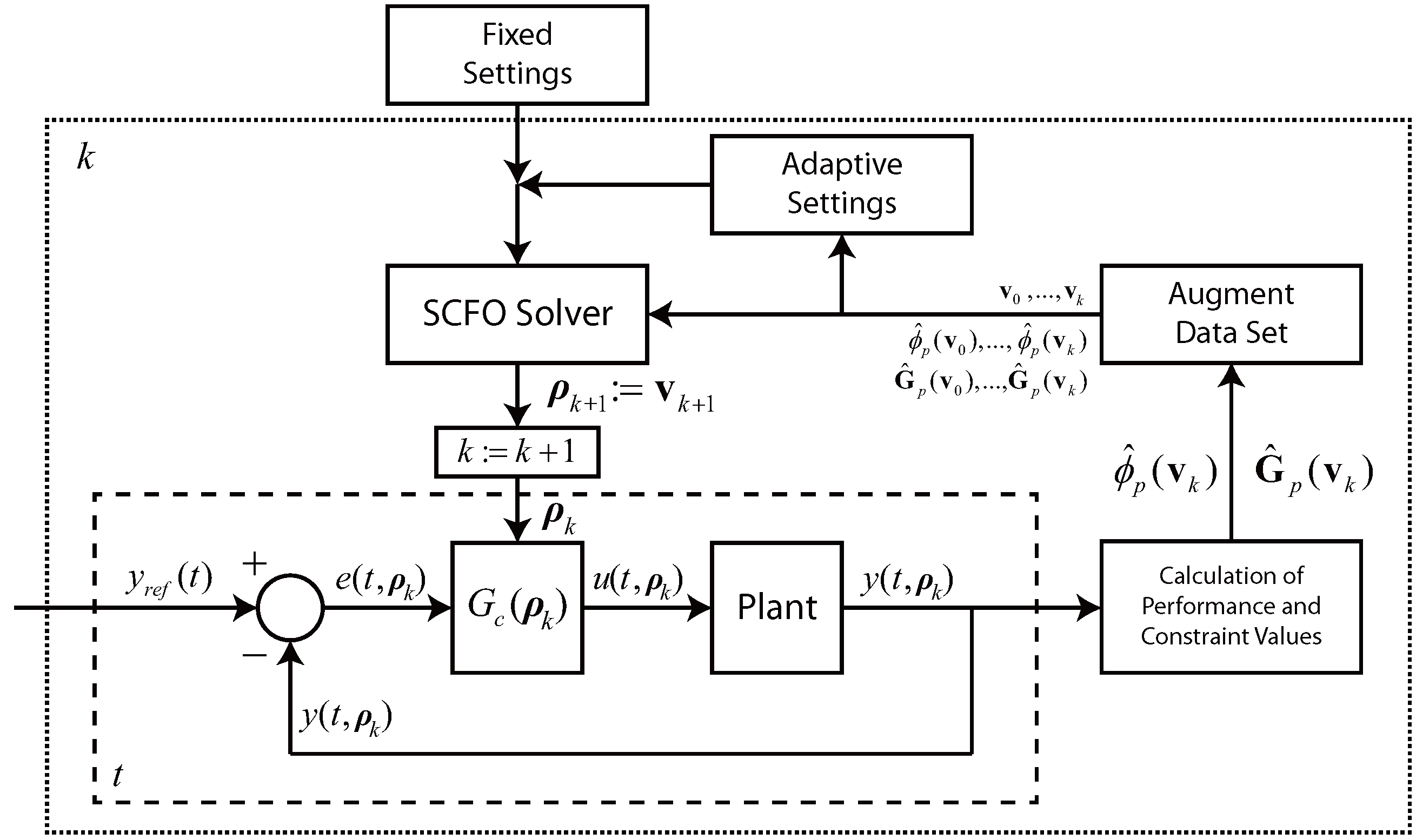
where the majority of the configuration is fixed once and for all, while the measurements act as the true iterative components, with the full set of measured data being fed to the solver at each iteration, after which it does all of the necessary computations and outputs the next RTO input to be applied. This is illustrated for the ICT context in Figure 3 (as an extension of Figure 1).

The natural price to pay for such simplicity of implementation is, not surprisingly, the complexity of configuration. Table 1 provides a summary of all of the configuration components, how they are set, and the justifications for these settings. Noting that most of these settings are relatively simple and do not merit further discussion, we now turn our focus to those that do.

Figure 3. The iterative tuning scheme, where the results obtained after each closed-loop experiment on the plant (denoted by the dashed lines) are sent to the RTO loop (denoted by the dotted box), which then appends these data to previous data and uses the full data set to prompt the SCFO solver, as well as to update any data-driven adaptive settings (we refer the reader to Table 1 for which settings are fixed and which are adaptive).

Figure 3. The iterative tuning scheme, where the results obtained after each closed-loop experiment on the plant (denoted by the dashed lines) are sent to the RTO loop (denoted by the dotted box), which then appends these data to previous data and uses the full data set to prompt the SCFO solver, as well as to update any data-driven adaptive settings (we refer the reader to Table 1 for which settings are fixed and which are adaptive).

Table 1. Summary of SCFO configuration settings for the ICT problem.

Solver Setting	Chosen As	Justification	Type
Initialization	$n_{\mathit{\rho }}+1$ closed-loop experiments	See Section 3.1	–
Optimization target	Scaled gradient descent	See Section 3.2	Adaptive
Noise statistics	Initial experiments at ${\mathit{\rho }}_0$	See Section 3.3	Fixed
Constraint concavity	None assumed	No reason for assuming this property in ICT context	Fixed
Constraint relaxations	None assumed	For simplicity (should be added if some constraints are soft)	Fixed
Cost certainty	Cost function is uncertain	The performance metric is an unknown function of ρ	Fixed
Structural assumptions	Locally quadratic structure	Recommended choice for general RTO problem [17]	Fixed
Minimal-excitation radius	$0.01\left({\mathit{\rho }}_1^U-{\mathit{\rho }}_1^L\right)$	Recommended choice for general RTO problem [17]	Fixed
Lower and upper limits, ${\mathbf{v}}^L$ and ${\mathbf{v}}^U$	Controller-dependent or set adaptively	See Section 3.4	Fixed/Adaptive
Lipschitz and quadratic bound constants	Initial data-driven guess followed by adaptive setting	See Section 3.5	Fixed/Adaptive
Scaling bounds	Problem-dependent; easily chosen	See [17]	Fixed
Maximal allowable adaptation step, $\Delta {\mathbf{v}}_{max}$	$0.1{\left({\mathit{\rho }}^U-{\mathit{\rho }}^L\right)}^T$	Recommended choice for general RTO problem [17]	Fixed

Table 1. Summary of SCFO configuration settings for the ICT problem.

Solver Setting	Chosen As	Justification	Type
Initialization	$n_{\mathit{\rho }}+1$ closed-loop experiments	See Section 3.1	–
Optimization target	Scaled gradient descent	See Section 3.2	Adaptive
Noise statistics	Initial experiments at ${\mathit{\rho }}_0$	See Section 3.3	Fixed
Constraint concavity	None assumed	No reason for assuming this property in ICT context	Fixed
Constraint relaxations	None assumed	For simplicity (should be added if some constraints are soft)	Fixed
Cost certainty	Cost function is uncertain	The performance metric is an unknown function of ρ	Fixed
Structural assumptions	Locally quadratic structure	Recommended choice for general RTO problem [17]	Fixed
Minimal-excitation radius	$0.01\left({\mathit{\rho }}_1^U-{\mathit{\rho }}_1^L\right)$	Recommended choice for general RTO problem [17]	Fixed
Lower and upper limits, ${\mathbf{v}}^L$ and ${\mathbf{v}}^U$	Controller-dependent or set adaptively	See Section 3.4	Fixed/Adaptive
Lipschitz and quadratic bound constants	Initial data-driven guess followed by adaptive setting	See Section 3.5	Fixed/Adaptive
Scaling bounds	Problem-dependent; easily chosen	See [17]	Fixed
Maximal allowable adaptation step, $\Delta {\mathbf{v}}_{max}$	$0.1{\left({\mathit{\rho }}^U-{\mathit{\rho }}^L\right)}^T$	Recommended choice for general RTO problem [17]	Fixed

3.1. Solver Initialization

Prior to attempting to solve Problem (1), it is strongly recommended that the problem be well-scaled with respect to both the RTO inputs and outputs. For the former, this means that:

$$v_1^U-v_1^L\approx v_2^U-v_2^L\approx ...\approx v_{n_v}^U-v_{n_v}^L\approx 1$$

where “≈” may be read as “on the same order of magnitude as”. For the RTO outputs, it is advised that both the cost and constraint functions are such that their values vary on the magnitude of ${10}^0$. Once this is done, one may proceed to initialize the data set.

As the solver needs to compute gradient estimates directly from measured data, it is usually needed to generate the $n_v+1$ measurements (whose corresponding RTO input values should be well-poised for linear regression) necessary for a rudimentary (linear) gradient estimate (see, e.g., [25,32]). In the case that previous measurements are already available (e.g., from experimental studies carried out prior to optimization), one may be able to avoid this step partially or entirely.

We will, for generality, assume the case where no previous data are available. We will also assume that the initial point, ${\mathbf{v}}_0:={\mathit{\rho }}_0$, has been obtained by some sort of controller design technique. In addition, we require that the initial design satisfy ${\mathbf{G}}_p({\mathbf{v}}_0)\prec \mathbf{0}$, $\mathbf{G}({\mathbf{v}}_0)\prec \mathbf{0}$, and ${\mathbf{v}}^L\prec {\mathbf{v}}_0\prec {\mathbf{v}}^U$—this is expected to hold intrinsically, since one would not start optimizing performance prior to having at least one design that is known to meet the required constraints with at least some safety margin. The next step is then to generate $n_v$ additional measurements, i.e., to run $n_v$ ($n_{\rho }$) closed-loop experiments on the plant.

A simple initialization method would be to perturb each controller parameter one at a time, as this would produce a well-poised data set with sufficient excitation in all input directions, thereby making the task of estimating the plant gradient possible. However, such a scheme could be wasteful, especially for ICT problems with many parameters to be tuned. One alternative would be to use smart, model-based initializations [25], but this would require having a plant model. In the case of no model, we propose to use a “smart” perturbation scheme that attempts to begin optimizing performance during the initialization phase, and refer the reader to the appendix for the detailed algorithm.

3.2. The Optimization Target

The target, ${\mathbf{v}}_{k+1}^{*}$, represents a nominal optimum provided by any standard RTO algorithm that is coupled with the SCFO solver and, as such, actually represents the choice of algorithm. This choice is important as it affects performance, with some of the results in [16] suggesting that coupling the SCFO with a “strong” RTO algorithm (e.g., a model-based one) can lead to faster convergence to the optimum. However, the choice is not crucial with respect to the reliability of the overall scheme, and so one does not need to be overly particular about what RTO algorithm to use, but should prefer one that generally guides the adaptations in the right direction.

For the sake of simplicity, the algorithm adopted in this work is the (scaled) gradient descent with a unit step size:

$${\mathbf{v}}_{k+1}^{*}={\mathbf{v}}_k-{\mathbf{H}}_k^{†}\nabla {\widehat{\varphi }}_p({\mathbf{v}}_k)$$

(14)

where both ${\mathbf{H}}_k$ and $\nabla {\widehat{\varphi }}_p({\mathbf{v}}_k)$ are data-driven estimates. We refer the reader to the appendix for how these estimates are obtained.

3.3. The Noise Statistics

Obtaining the statistics (i.e., the probability distribution function, or PDF) for the stochastic error terms δ in Equations (3) and (7) is particularly challenging in the ICT context. One reason for this is that these terms do not have an obvious physical meaning, as both Equations (3) and (7), which model the observed performance/constraint values as a sum of a deterministic and stochastic component, are approximations. Furthermore, even if this model were correct, the actual computation of an accurate PDF would likely require a number of closed-loop experiments on the plant that would be judged as excessive in practice.

As will be shown in the first two case studies of Section 4, some level of engineering approximation becomes inevitable in obtaining the PDF for an experimental system. The basic procedure advocated here is to carry out a certain (economically allowable) number of repeated experiments for ${\mathbf{v}}_0:={\mathit{\rho }}_0$ prior to the initialization step. In the case where each experiment is expensive (or time consuming) and the total acceptable number is low, one may approximate the δ term by modeling the observed values by a zero-mean normal distribution with a standard deviation equal to that of the data. If the experiments are cheap and a fairly large number (e.g., a hundred or more) is allowed, then the observed data may be offset by its mean and then fed directly into the solver (as the solver builds an approximate PDF directly from the fed noise data).

3.4. Lower and Upper Input Limits

Providing proper lower and upper limits ${\mathbf{v}}^L$ and ${\mathbf{v}}^U$ can be crucial to solver performance. As already stated, for the ICT problem these are simply ${\mathbf{v}}^L:={\mathit{\rho }}^L$ and ${\mathbf{v}}^U:={\mathit{\rho }}^U$, but, as these values may not be obvious for certain controller designs, the user may use adaptive limits that are redefined at each iteration k:

$$\begin{array}{c}{\mathit{\rho }}_k^L:={\mathit{\rho }}_k-\mathbf{0}.\mathbf{5}\hfill \\ {\mathit{\rho }}_k^U:={\mathit{\rho }}_k+\mathbf{0}.\mathbf{5}\hfill \end{array}$$

(15)

As the solver can never actually converge to an optimum that touches these limits, the resulting problem is essentially unconstrained with respect to them, thereby allowing us to configure the solver without affecting the optimality properties of the problem. We note that, while one could use very conservative choices and not adapt them (e.g., ${\mathit{\rho }}^L:=-\mathbf{1},\mathbf{000}$ and ${\mathit{\rho }}^U:=\mathbf{1},\mathbf{000}$), this is not recommended as it would introduce scaling issues into the solver’s subroutines.

3.5. Lipschitz and Quadratic Bound Constants

The solver requires the user to provide the Lipschitz constants (denoted by κ) for all of the functions ${\varphi }_p$, ${\mathbf{G}}_p$ and $\mathbf{G}$. These are implicitly defined as:

$${\displaystyle {\underline{\kappa }}_{\varphi ,i}<\frac{\partial {\varphi }_p}{\partial v_i}{|}_{\mathbf{v}}<{\overline{\kappa }}_{\varphi ,i},{\underline{\kappa }}_{p,i}<\frac{\partial g_p}{\partial v_i}{|}_{\mathbf{v}}<{\overline{\kappa }}_{p,i},{\underline{\kappa }}_i<\frac{\partial g}{\partial v_i}{|}_{\mathbf{v}}<{\overline{\kappa }}_i}$$

for all $\mathbf{v}\in \{\mathbf{v}:{\mathbf{v}}^L⪯\mathbf{v}⪯{\mathbf{v}}^U\}$. Quadratic bound constants (denoted by M) on the cost function are also required and are implicitly defined as:

$${\underline{M}}_{ij}<\frac{{\partial }^2{\varphi }_p}{\partial v_i\partial v_j}{|}_{\mathbf{v}}<{\overline{M}}_{ij},\forall \mathbf{v}\in \{\mathbf{v}:{\mathbf{v}}^L⪯\mathbf{v}⪯{\mathbf{v}}^U\}$$

For $\mathbf{G}$, which is easily evaluated numerically, we note that the choice is simple since one can, in many cases, compute these values prior to any implementation.

For ${\kappa }_{\varphi ,i}$, ${\kappa }_{p,i}$ and $M_{ij}$, the choice is a very difficult one. This is especially true for the ICT problem, where such constants have no physical meaning, a trait that may make them easier to estimate for some RTO problems [16]. When a model of the plant is available, one may proceed to compute these values numerically for the modeled closed-loop behavior and then make the estimates more conservative (e.g., by applying a safety-factor scaling) to account for plant-model mismatch.

For the pure model-free case, we have no choice but to resort to heuristic approaches. As a choice of ${\kappa }_{\varphi ,i}$, we thus propose the following (very conservative) estimate based on the gradient estimate for the initial $n_v+1$ points (23):

$${\overline{\kappa }}_{\varphi ,i},{\underline{\kappa }}_{\varphi ,i}:=\pm 10{\parallel \nabla {\widehat{\varphi }}_p\parallel }_{\infty },i=1,...,n_v$$

as we expect these bounds to be valid unless $\parallel \nabla {\widehat{\varphi }}_p{\parallel }_{\infty }$ is small, which, however, would indicate that we are probably close to a zero-gradient stationary point already and would have little to gain by trying to optimize performance further if this point were a minimum.

A similar rule is applied to estimate ${\kappa }_{p,i}$, with:

$${\overline{\kappa }}_{p,i},{\underline{\kappa }}_{p,i}:=\pm 2{\parallel \nabla {\widehat{g}}_p\parallel }_{\infty },i=1,...,n_v$$

where the estimate $\nabla {\widehat{g}}_p$ is obtained in the same manner as in Equation (23). The choice of 2, as opposed to 10, is made for performance reasons, as making ${\kappa }_{p,i}$ too conservative can lead to very slow progress in improving performance—this is expected to scale linearly, i.e., if the choice of $\pm 2\parallel \nabla {\widehat{g}}_p{\parallel }_{\infty }$ leads to a realization that converges in 20 runs, the choice of $\pm 10\parallel \nabla {\widehat{g}}_p{\parallel }_{\infty }$ may lead to one that converges in 100. Note, however, that this way of defining the Lipschitz constants does not have the same natural safeguard as it does for the cost, and it may happen that $\parallel \nabla {\widehat{g}}_p{\parallel }_{\infty }\approx 0$ at the initial point even though the gradient may be quite large in the neighborhood of the optimum. When this is so, an alternate heuristic choice is to set:

$${\overline{\kappa }}_{p,i},{\underline{\kappa }}_{p,i}:=\pm 2\frac{-{\underline{g}}_p}{v_i^U-v_i^L},i=1,...,n_v$$

where ${\underline{g}}_p$ denotes the smallest value that the constraint can take in practice, with ${\underline{g}}_p\le g_p(\mathbf{v}),\forall \mathbf{v}\in \{\mathbf{v}:{\mathbf{v}}^L⪯\mathbf{v}⪯{\mathbf{v}}^U\}$. Combining the two, one may then use the heuristic rule:

$${\overline{\kappa }}_{p,i},{\underline{\kappa }}_{p,i}:=\pm 2max\left(\parallel \nabla {\widehat{g}}_p{\parallel }_{\infty },\frac{-{\underline{g}}_p}{v_i^U-v_i^L}\right),i=1,...,n_v$$

However, it may still occur that this choice is not conservative enough. This lack of conservatism may be proven if a given constraint, $g_p(\mathbf{v})\le 0$, is violated for one of the runs, since sufficiently conservative Lipschitz estimates will usually guarantee that this is not the case (provided that the noise statistics are sufficiently accurate). As such, the following adaptive refinement of the Lipschitz constants is proposed to be done online when/if the constraint is violated with sufficient confidence:

$$g_p({\mathbf{v}}_k)\ge 3{\sigma }_g\to {\overline{\kappa }}_{p,i}:=2{\overline{\kappa }}_{p,i},{\underline{\kappa }}_{p,i}:=2{\underline{\kappa }}_{p,i}$$

where ${\sigma }_g$ represents the estimated standard deviation of the non-repeatability noise term, δ, for $g_p$.

For the quadratic bound constants M, which represent lower and upper bounds on the second derivatives of ${\varphi }_p$, we propose to use the estimate of the Hessian, ${\mathbf{H}}_k$, as obtained in Section 3.2 (see Appendix), together with a safety factor, η, to define the bounds at each iteration k as:

$${\overline{M}}_{ij},{\underline{M}}_{ij}:=H_{k,ij}\pm \eta \left|H_{k,ij}\right|$$

(16)

with η initialized as 1. Since such a choice may also suffer from a lack of conservatism, an adaptive algorithm for η is put into place. Since a common indicator of choosing M values that are not conservative enough is the failure to decrease the cost between consecutive iterations, the following law is proposed for any iterations where the solver applied the SCFO conditions but increased (with sufficient confidence) the value of the cost [17]:

• If ${\widehat{\varphi }}_p({\mathbf{v}}_k)-4{\sigma }_{\varphi }\ge \underset{i=0,...,k-1}{min}{\widehat{\varphi }}_p({\mathbf{v}}_i)$, then set $\eta :=\eta +1$;
• otherwise, set $\eta :=\eta -0.5$, with $\eta <0\to \eta :=0$,

where ${\sigma }_{\varphi }$ is the estimated standard deviation for the non-repeatability noise term in the measurement of $J_k$. The essence of this update law is to make M more conservative (by increasing η) whenever the performance is statistically likely to have increased in the recent adaptation and to relax the conservatism otherwise, though at only twice the rate that it would be increased. Such a scheme essentially ensures that the M constants become conservative enough to continually guarantee improved performance with an increasing number of iterations.

4. Case Studies

The proposed method was applied to four different problems, of which the first two are of particular interest, as they were carried out on experimental systems and demonstrate the reliability and effectiveness of the proposed approach when applied in settings where neither the plant nor the non-repeatability noise terms are known. Of these two, the first represents a typical batch scenario with fairly slow dynamics and time-consuming, expensive experiments for which an MPC controller is employed (Section 4.1), while the latter represents a much faster mechanical system, where the optimization of the controller parameters for a general fixed-order controller must be carried out quickly due to real-time constraints, but where a single run is inexpensive (Section 4.2).

The last two studies, though lacking the experimental element, are nevertheless of interest as they make a link with similar work carried out by other researchers (Section 4.3) and generalize the method to systems of controllers with an additional challenge in the form of an output constraint (Section 4.4). In both of these cases, we have chosen to simplify things by assuming to know the noise statistics of the relevant δ terms and to let the repeatability assumption hold exactly.

In each of the four studies, we have used the configuration proposed in Section 3 and so will not repeat these details here. However, we will highlight those components of the configuration that are problem-dependent and will explain how we obtained them for each case.

4.1. Batch-to-Batch Temperature Tracking in a Stirred Tank

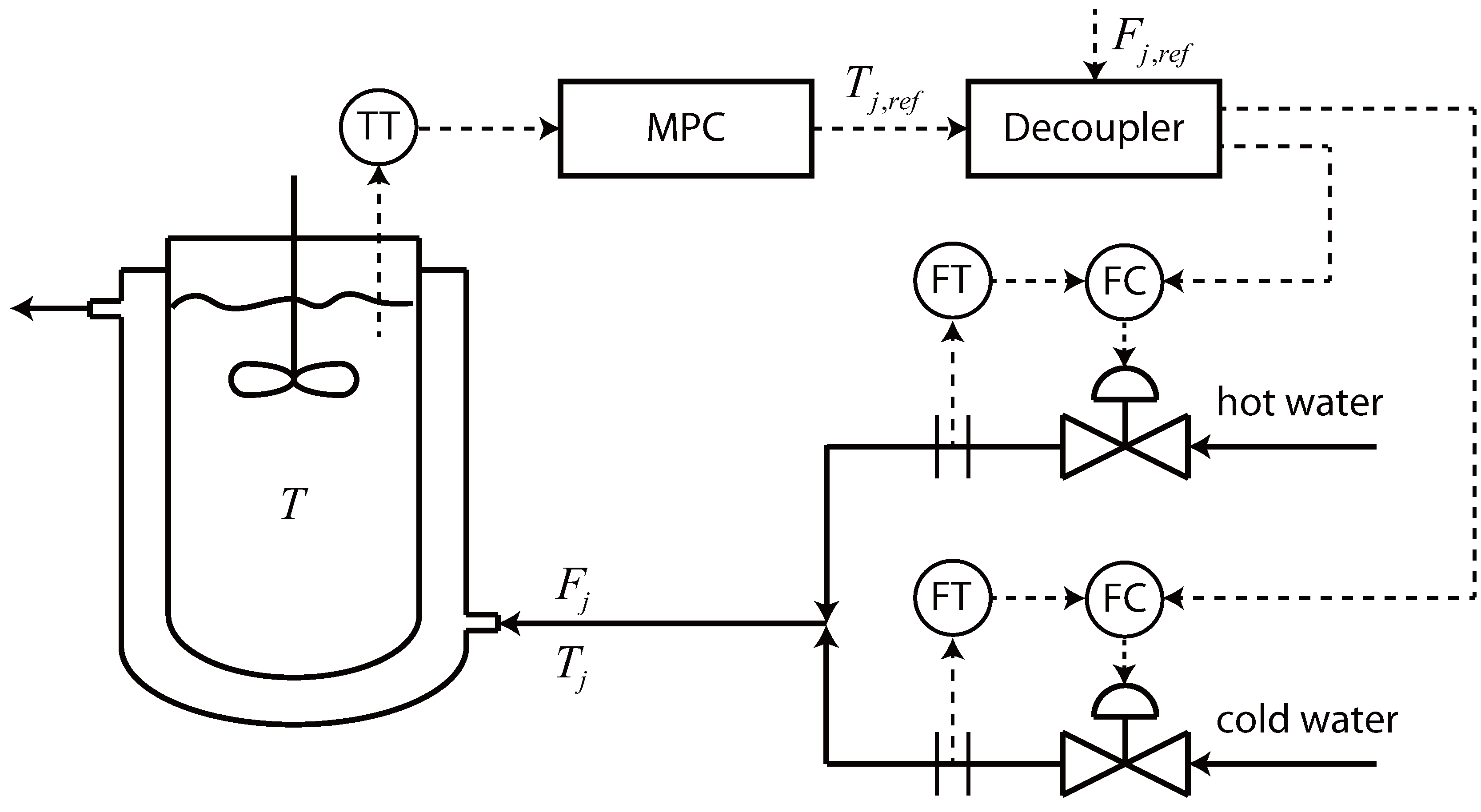
The plant in question is a jacketed stirred water tank, where a cascade system is used to control the temperature inside the tank by having an MPC controller manipulate the setpoint temperature of the jacket inlet, which is, in turn, tracked by a decoupled system of two PI controllers that manipulate the flow rates of the hot and cold water streams that mix to form the jacket inlet (Figure 4). As this system is essentially identical to what has been previously reported [33], we refer the reader to the previous work for all of the implementation details.

Figure 4. Schematic of the jacketed stirred tank and the cascade control system used to control the water temperature inside the tank. The reference ($F_{j,ref}$) for the water flow to the jacket ($F_j$) was fixed at 2 L/min.

Figure 4. Schematic of the jacketed stirred tank and the cascade control system used to control the water temperature inside the tank. The reference ($F_{j,ref}$) for the water flow to the jacket ($F_j$) was fixed at 2 L/min.

As the task of tracking an “optimal” temperature profile is fairly common in batch processes and the failure to do so well can lead to losses in product quality, a natural ICT problem arises in these contexts as it is desired that the temperature stay as close to the prescribed optimal setpoint trajectory as possible. In this particular case study, the controller that is tasked with this job is the MPC controller, whose tunable parameters include:

• the output weight that controls the trade-off between controller aggressiveness and output tracking,
• the bias update filter gain, which acts to ensure offset-free tracking,
• the control and prediction horizons that dictate how far ahead the MPC attempts to look and control,

all of which act to change the objective function at the heart of the MPC controller [33]. For this problem, we decided to vary the output weight between 0.1 and 10 (i.e., covering three orders of magnitude) and defined its logarithm as the first tunable variable, ${\rho }_1$. Our reason for choosing the logarithm, instead of the actual value, was due to the sensitivity of the performance being more uniform with respect to the magnitude difference between the priorities given to controller aggressiveness and output tracking (e.g., changing the output weight from 0.1 to 1.0 was expected to have a similar effect as changing it from 1.0 to 10). The bias update filter gain, defined as the second variable ${\rho }_2$, was forced to vary between 0 and 1 by definition. The control and prediction horizons, m and n, were both allowed to vary anywhere between 2 and 50 and, as this variance was on the magnitude of ${10}^2$, were divided by 100 so as to have comparable scaling with the other parameters, with ${\rho }_3\stackrel{\Delta }{=}m/100$ and ${\rho }_4\stackrel{\Delta }{=}n/100$. We note as well that the horizons were constrained to be integers, whereas the solver provided real numbers, and so any answer provided by the solver had to be rounded to the nearest integer to accommodate these constraints.

As this system was fairly slow/stable and controller aggressiveness was not really an issue and as there was no strong preference between using hot or cold water, the performance metric simply consisted of minimizing the tracking error (i.e., the general metric in Equation (5) with ${\lambda }_1:=1$ and ${\lambda }_2:={\lambda }_3:={\lambda }_4:=0$) over a batch time of $t_b=40$ min. The setpoint trajectory to be tracked consisted of maintaining the temperature at 52 °C for 10 min, cooling by 4 °C over 10 min, and then applying a quadratic cooling profile for the remainder of the batch. Each batch was initialized by setting the jacket inlet to 55 °C and starting the batch once the tank temperature rose to 52 °C.

The certain inequality constraint ${\rho }_3\le {\rho }_4$ was enforced as this was needed by definition—see Equation (9)—thereby contributing to yield the following ICT problem in RTO form:

$$\begin{array}{cc}\hfill \underset{\mathit{\rho }}{\mathrm{minimize}}& {\displaystyle \frac{1}{J_0}{\int }_0^{40}{\left[T_{ref}(t)-T(t,\mathit{\rho })\right]}^{2}dt}\hfill \\ \hfill \mathrm{subject}\mathrm{to}& {\rho }_3-{\rho }_4\le 0\hfill \\ & -1\le {\rho }_1\le 1\hfill \\ & 0\le {\rho }_2\le 1\hfill \\ & 0.02\le {\rho }_3\le 0.50\hfill \\ & 0.02\le {\rho }_4\le 0.50\hfill \end{array}\begin{array}{c}\left.\begin{array}{c}\hfill \end{array}\right\}{\varphi }_p(\mathbf{v})\hfill \\ \left.\begin{array}{c}\hfill \end{array}\right\}\mathbf{G}(\mathbf{v})⪯\mathbf{0}\hfill \\ \left.\begin{array}{c}\hfill \\ \hfill \\ \hfill \\ \hfill \end{array}\right\}{\mathbf{v}}^L⪯\mathbf{v}⪯{\mathbf{v}}^U\hfill \end{array}$$

(17)

where we scaled the performance metric by dividing by its initial value (thereby giving us a base performance metric value of 1, which was then to be lowered). We also note that in practice measurements were collected every 3 s, and so the integral of the squared error was evaluated discretely. The initial parameter set was chosen, somewhat arbitrarily, as ${\mathit{\rho }}_0:={[-0.70.50.30.3]}^T$.

Prior to solving (17), we first solved an easier problem where ${\rho }_3$ and ${\rho }_4$ were fixed at their initial values and only ${\rho }_1$ and ${\rho }_2$ were optimized over (these two parameters being expected to be the more influential of the four):

$$\begin{array}{cc}\hfill \underset{{\rho }_1,{\rho }_2}{\mathrm{minimize}}& {\displaystyle \frac{1}{J_0}{\int }_0^{40}{\left[T_{ref}(t)-T(t,{\rho }_1,{\rho }_2)\right]}^{2}dt}\hfill \\ \hfill \mathrm{subject}\mathrm{to}& -1\le {\rho }_1\le 1\hfill \\ & 0\le {\rho }_2\le 1\hfill \end{array}\begin{array}{c}\left.\begin{array}{c}\hfill \end{array}\right\}{\varphi }_p(\mathbf{v})\hfill \\ \left.\begin{array}{c}\hfill \\ \hfill \end{array}\right\}{\mathbf{v}}^L⪯\mathbf{v}⪯{\mathbf{v}}^U\hfill \end{array}$$

(18)

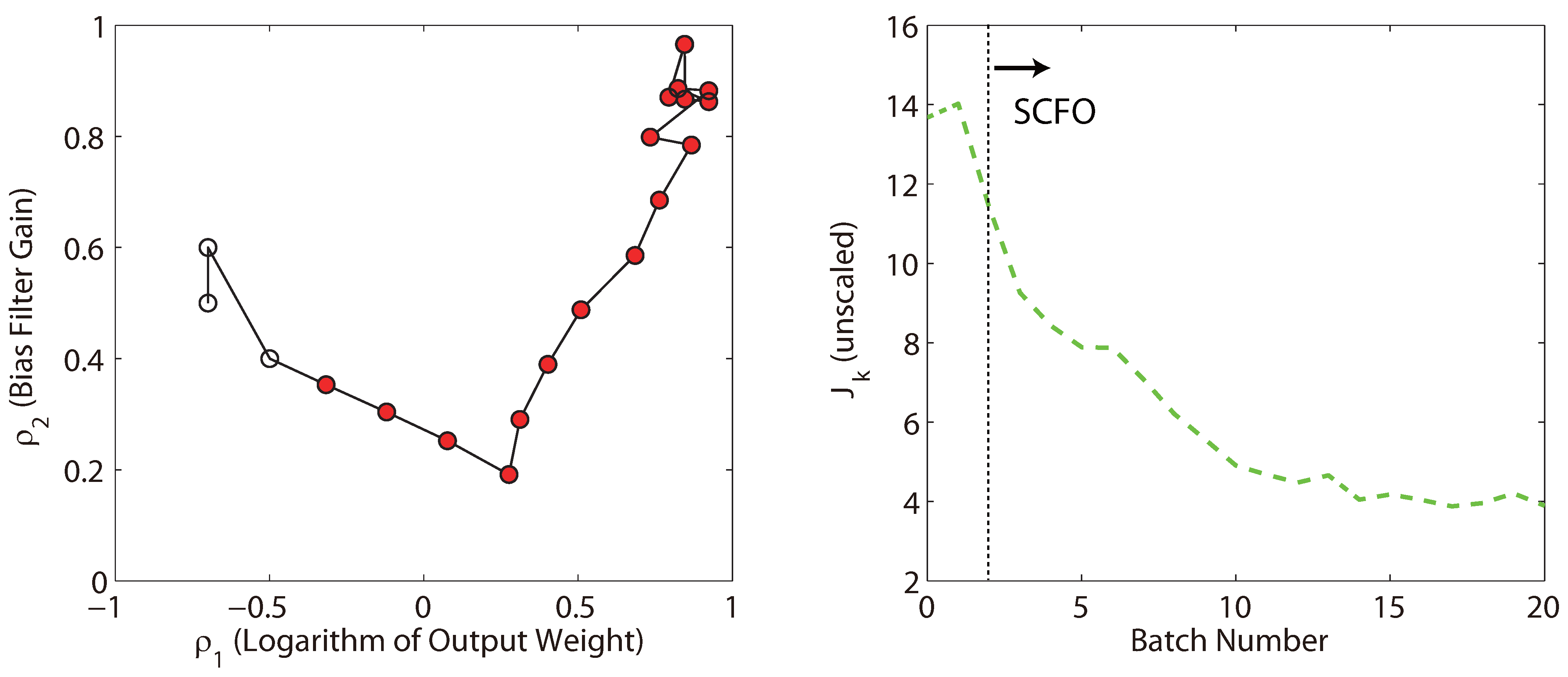
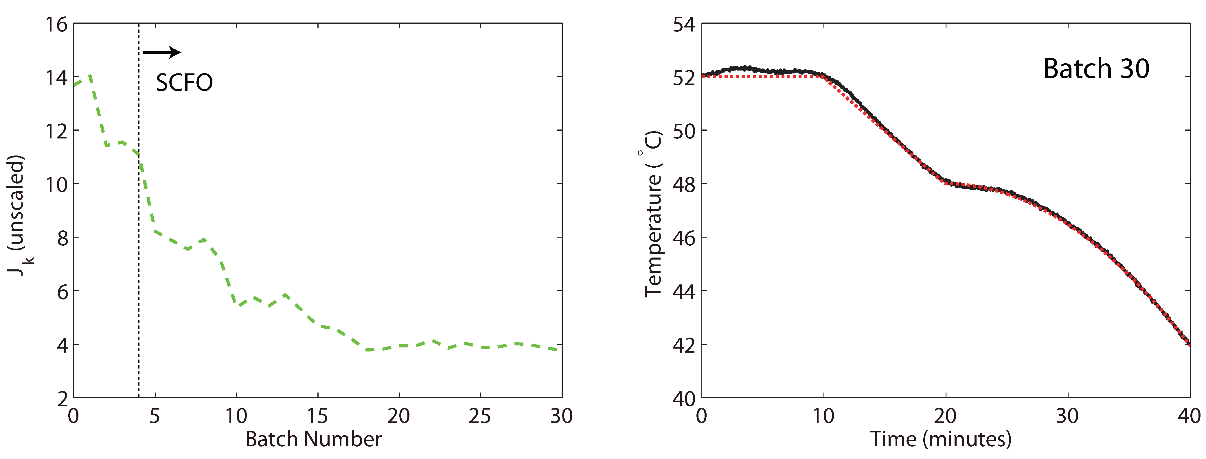
In order to approximate the non-repeatability noise term for the performance, a total of 8 batches were run with the initial parameter set ${\mathit{\rho }}_0$, with the (unscaled) performance metric values obtained for those experiments being: 13.45, 13.31, 13.46, 14.25, 13.80, 13.44, 13.72 and 13.98 (their mean then being taken as the scaling term, $J_0$). Rather than attempt to run more experiments, which, though it could have improved the accuracy of our approximation, would have required even more time (each batch already requiring 40 min, with an additional 20–30 min of inter-batch preparation), we chose to approximate the statistics of the non-repeatability noise term by a zero-mean normal distribution with the standard deviation of the data, i.e., 0.32.

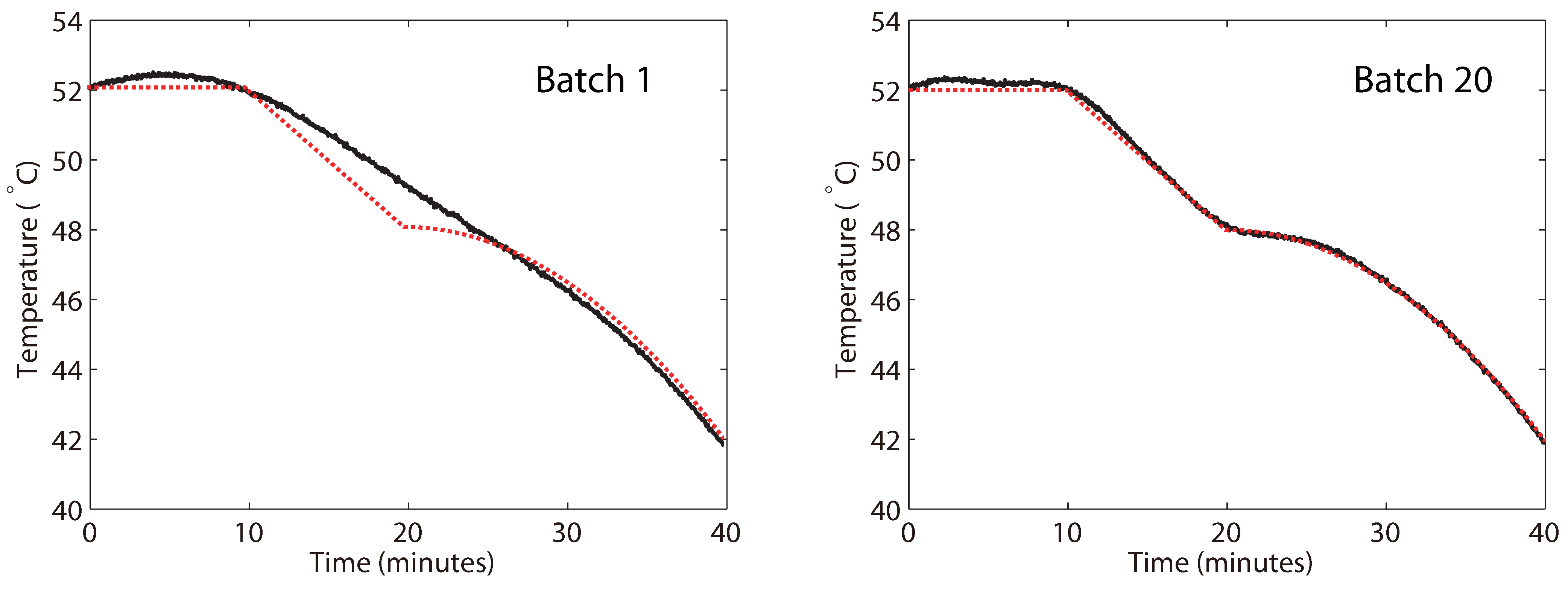
The map of the parameter adaptations and the values of the measured performance metric are given in Figure 5, with a visual comparison of the tracking before and after optimization given in Figure 6. It is seen that the majority of the improvement is obtained by about the tenth batch, with only minor improvements afterwards, and that monotonic improvement of the control performance is more or less observed.

Figure 5. The parameter adaptation plot (left) and the measured performance metric (right) for the solution of Problem (18). Hollow circles on the left indicate batches that were carried out as part of the initialization (prior to applying the solver). Likewise, the dotted vertical line on the right shows the iteration past which the parameter adaptations were dictated by the SCFO solver.

Figure 5. The parameter adaptation plot (left) and the measured performance metric (right) for the solution of Problem (18). Hollow circles on the left indicate batches that were carried out as part of the initialization (prior to applying the solver). Likewise, the dotted vertical line on the right shows the iteration past which the parameter adaptations were dictated by the SCFO solver.

Figure 6. The visual improvement in the temperature profile tracking from Batch 1 to Batch 20. The dotted (red) lines denote the setpoint, while the solid (black) lines denote the actual measured temperature.

Figure 6. The visual improvement in the temperature profile tracking from Batch 1 to Batch 20. The dotted (red) lines denote the setpoint, while the solid (black) lines denote the actual measured temperature.

We also note that the solution obtained by the solver is very much in line with what an engineer would expect for a system with slow dynamics such as this one, in that one should increase both the output weight so as to have better tracking and set the bias update filter gain close to its maximal value (both of these actions could have potentially negative effects for faster, less stable systems, however). As such, the solution is not really surprising, but it is still encouraging that a method with absolutely no knowledge embedded into it has been able to find the same in a relatively low number of experiments. It is also interesting to note that the non-repeatability noise in the measured performance metric originally puts us on the wrong track, as increasing the bias update filter gain does not improve the observed performance for Batch 1, though it probably should, and so the solver then spends the first 6 adaptations decreasing the bias filter gain in the belief that doing so should improve performance. However, it is able to recover by Batch 7 and to go in the right direction afterwards—this is likely due to the internal gradient estimation algorithm of the solver having considered all of the batches and having thereby decoupled the effects of the two parameters.

Problem (17) was then solved by similar means, though we used all of the data obtained previously to help “warm start” the solver. As the results were similar to what was obtained for the two-parameter case, we only give the measured performance metric values and the temperature profile at the final batch in Figure 7. We also note that the parameter values at the final batch were ${\mathit{\rho }}_{30}={[0.890.950.070.12]}^T$, from which we see that, while all four variables were clearly adapted and the solver chose to lower both the control and prediction horizons, any extra performance gains from doing this (if any) appear to have been marginal when compared to the simpler two-parameter problem. This is also in line with our intuition (i.e., that the output weight and bias filter gain are more important) and reminds us of a very important RTO concept: just because one has many variables that one can optimize over does not mean that one should, as RTO problems with more optimization variables are generally expected to converge slower and, as seen here, may not be worth the effort.

Figure 7. The measured performance metric for the solution of Problem (17), together with the tracking obtained for the final batch.

Figure 7. The measured performance metric for the solution of Problem (17), together with the tracking obtained for the final batch.

4.2. Periodic Setpoint Tracking in a Torsional System

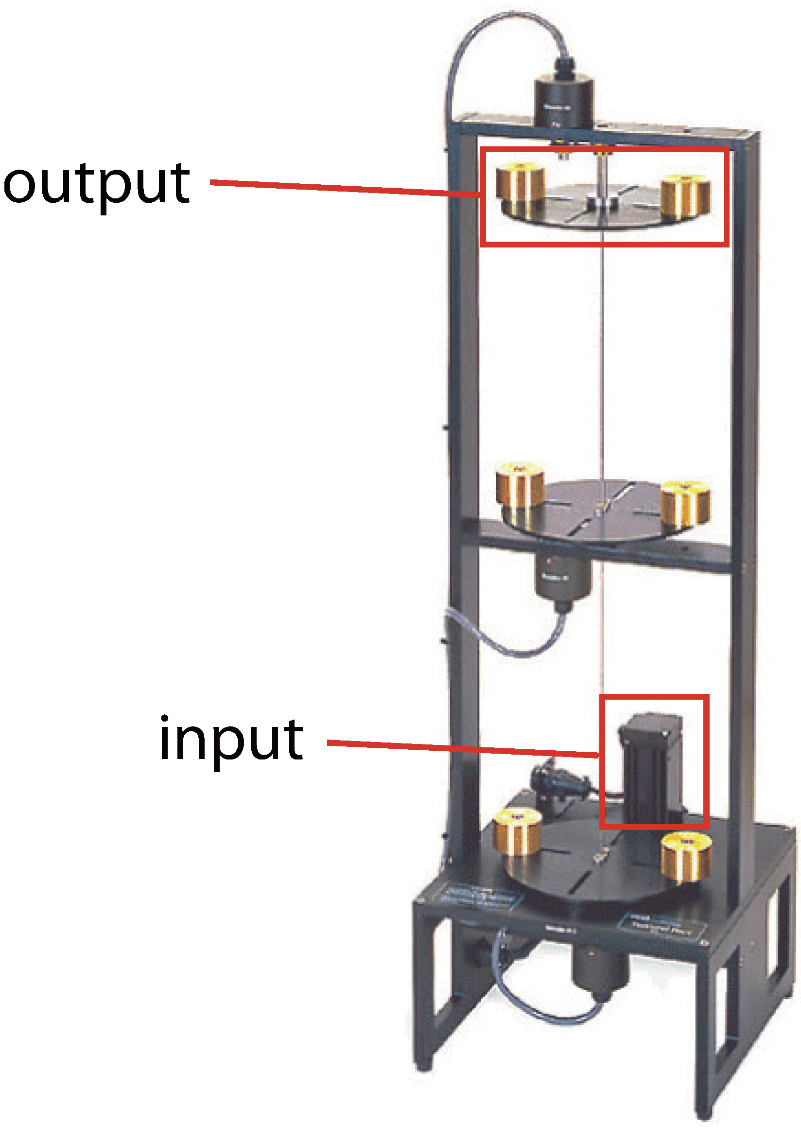
In this study, we consider the three-disk torsional system shown in Figure 8 (the technical details of which may be found in [34]). Here, the control input is defined as the voltage of the motor located near the bottom of the system, with the control output taken as the angular position of the top disk.

Figure 8. The ECP 205 torsional system.

Figure 8. The ECP 205 torsional system.

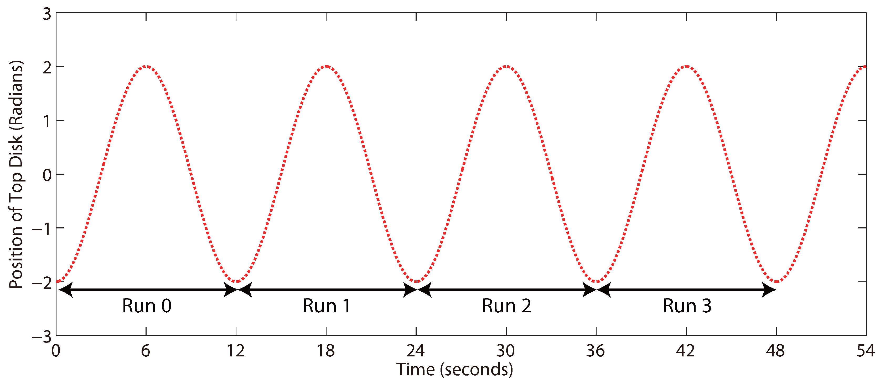
To define an ICT problem, we generalize the idea of a “run” or a “batch” as seen in the previous example and consider, instead, a “window” of a periodic sinusoidal trajectory defined by:

$${\displaystyle y_{ref}(t)=-2\cos \frac{\pi t}{6}}$$

with t given in seconds. As the same trajectory is repeated every 12 s, we can essentially consider each 12-second window as a “run” (or a “batch”), as shown in Figure 9, and adapt the relevant controller parameters in the sampling time period between two consecutive windows.

Figure 9. The generalization of “run-to-run” tuning to a system with a periodic setpoint trajectory. Only the setpoint is given here.

Figure 9. The generalization of “run-to-run” tuning to a system with a periodic setpoint trajectory. Only the setpoint is given here.

Not surprisingly, this presents a computational challenge, as the sampling time for this system is only 60 ms, which is, with the current version of the solver, insufficient—the solver needing at least a few seconds to provide a new choice of parameters. While a much simpler implementation that satisfies this real-time constraint has already been successfully carried out on the same system [20], we choose to apply the methodology presented in this paper by using a wait-and-synchronize approach. Here, the solver takes all of the available data and starts its computations, with no adaptation of the parameters being done until the solver’s computations are finished. Afterwards, the solver waits until these new parameters are applied and the results for the corresponding run obtained, after which the new data is fed into the solver and the cycle restarts. The noted drawback of this approach is that we have to wait, on average, 2–3 runs (24–36 s) for an adaptation to take place, although the positive side of this is that the resulting data is generally less noisy due to the repeated experiments.

The controller employed is the discrete fixed-order controller given in Equation (10), with the numerator and denominator coefficients being the (five) tuned parameters. The performance metric used is, again, a case of the general metric (5), but this time equal priority is given to tracking, controller aggressiveness, and the smoothness of the output trajectory, with ${\lambda }_1:={\lambda }_3:={\lambda }_4:=1$ and ${\lambda }_2:=0$.

As the poles of the controller are also being adapted (due to the adaptation of the denominator coefficients), controller stability constraints, as already derived in Equations (11) and (12), are added to the ICT problem (with a tolerance of $\epsilon :=0.01$):

$$\begin{array}{c}|{\rho }_5|-0.99\le 0\hfill \\ |{\rho }_4-{\rho }_4{\rho }_5|-|1-{\rho }_5^2|+0.01\le 0\hfill \end{array}$$

and are recast into differentiable form (as the solver requires $\mathbf{G}$ to be differentiable):

$$\begin{array}{c}{\rho }_5-0.99\le 0\hfill \\ -{\rho }_5-0.99\le 0\hfill \\ {\rho }_4-{\rho }_4{\rho }_5-(1-{\rho }_5^2)+0.01\le 0\hfill \\ -{\rho }_4+{\rho }_4{\rho }_5-(1-{\rho }_5^2)+0.01\le 0\hfill \end{array}$$

where we have used $|{\rho }_5|\le 0.99\Rightarrow |1-{\rho }_5^2|=1-{\rho }_5^2$ in the reformulation of the second set.

The adaptive limits of Equation (15) are used to constrain the individual parameters, thereby leading to the (adaptive) ICT-RTO problem:

$$\begin{array}{cc}\hfill \underset{\mathit{\rho }}{\mathrm{minimize}}& {\displaystyle \frac{1}{100}{\int }_0^{12}\left({\left[y_{ref}(t)-y(t,\mathit{\rho })\right]}^2+{\dot{u}}^2(t,\mathit{\rho })+{\dot{y}}^2(t,\mathit{\rho })\right)dt}\hfill \\ \hfill \mathrm{subject}\mathrm{to}& {\rho }_5-0.99\le 0\hfill \\ & -{\rho }_5-0.99\le 0\hfill \\ & {\rho }_4-{\rho }_4{\rho }_5-(1-{\rho }_5^2)+0.01\le 0\hfill \\ & -{\rho }_4+{\rho }_4{\rho }_5-(1-{\rho }_5^2)+0.01\le 0\hfill \\ & {\rho }_{k,1}-0.5\le {\rho }_1\le {\rho }_{k,1}+0.5\hfill \\ & {\rho }_{k,2}-0.5\le {\rho }_2\le {\rho }_{k,2}+0.5\hfill \\ & {\rho }_{k,3}-0.5\le {\rho }_3\le {\rho }_{k,3}+0.5\hfill \\ & {\rho }_{k,4}-0.5\le {\rho }_4\le {\rho }_{k,4}+0.5\hfill \\ & {\rho }_{k,5}-0.5\le {\rho }_5\le {\rho }_{k,5}+0.5\hfill \end{array}\begin{array}{c}\left.\begin{array}{c}\hfill \end{array}\right\}{\varphi }_p(\mathbf{v})\hfill \\ \left.\begin{array}{c}\hfill \\ \hfill \\ \hfill \\ \hfill \end{array}\right\}\mathbf{G}(\mathbf{v})⪯\mathbf{0}\hfill \\ \left.\begin{array}{c}\hfill \\ \hfill \\ \hfill \\ \hfill \\ \hfill \end{array}\right\}{\mathbf{v}}^L⪯\mathbf{v}⪯{\mathbf{v}}^U\hfill \end{array}$$

(19)

where we scale the performance metric by ${10}^2$ so as to make it vary on the magnitude of ${10}^0$.

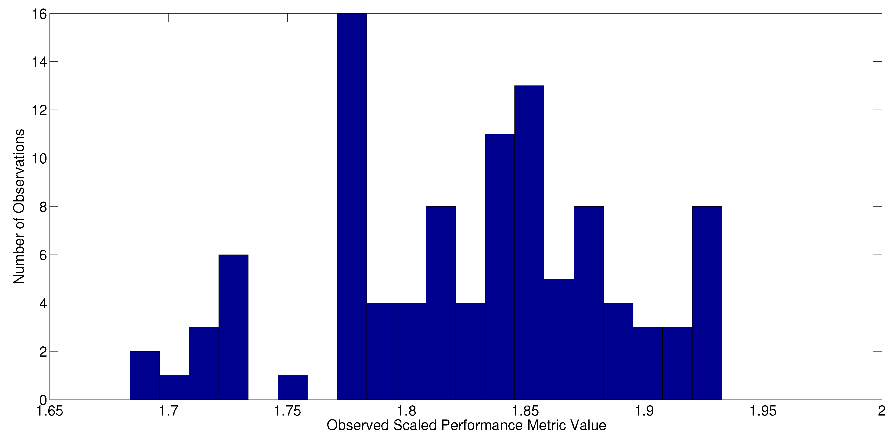
An initial parameter set of ${\mathit{\rho }}_0:={[1.002.77-2.601.000.50]}^T$ was chosen and corresponds to an ad hoc initial design found by a mix of both simulation and hand tuning. To estimate the noise statistics of the non-repeatability noise term in the performance metric, the system was operated at ${\mathit{\rho }}_0$ for 20 min, which produced a total of 100 performance metric measurements (see Figure 10). These were then offset by their mean to generate the estimated noise samples, with the latter being fed directly into the solver, which would then build an approximate distribution function for them.

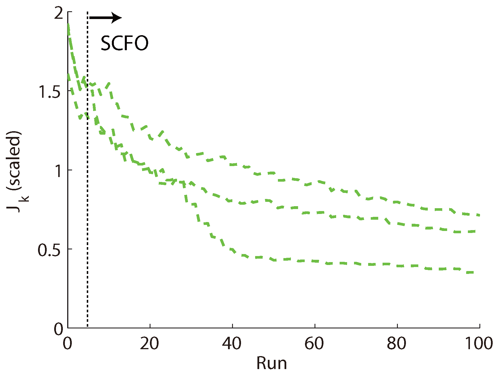
Problem (19) was solved a total of three times for 20 min of operation (100 runs), with the performance improvements for the three trials given in Figure 11 and the visual improvement for the middle case (“middle” with regard to the final performance metric value) given in Figure 12. We note the variability in convergence behavior for the three cases (both in terms of speed and the performance achieved after 100 runs), which was largely caused by the solver converging to different minima, but note as well that all three follow the same “reliable” trend, in that performance is always improved with a fairly consistent decrease in the metric value over the course of operation.

Figure 10. A twenty-bin histogram representation of the observed scaled performance metric values for a hundred runs with the initial parameter set (Problem (19)).

Figure 10. A twenty-bin histogram representation of the observed scaled performance metric values for a hundred runs with the initial parameter set (Problem (19)).

Figure 11. Performance improvement over 100 runs of operation for three different trials (dashed lines) of Problem (19).

Figure 11. Performance improvement over 100 runs of operation for three different trials (dashed lines) of Problem (19).

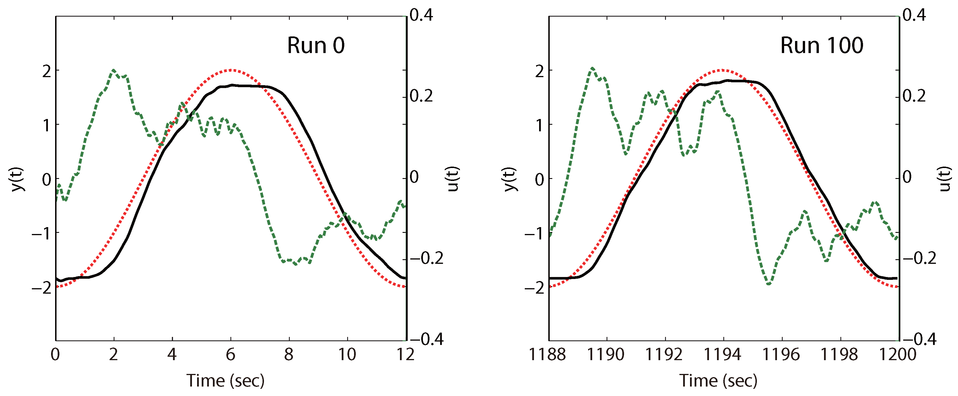
Figure 12. Difference in control input and output profiles between the first and final runs of Problem (19), with the dashed green line used to denote the input (motor voltage) values.

Figure 12. Difference in control input and output profiles between the first and final runs of Problem (19), with the dashed green line used to denote the input (motor voltage) values.

4.3. PID Tuning for a Step Setpoint Change

We consider the problem previously examined in [13,18], where the parameters of a PID controller are to be tuned for the closed-loop system given by:

$$Y(s)=\frac{G_{ref}(s)G_p(s)}{1+G_y(s)G_p(s)}{Y}_{ref}(s)$$

with the PID parameters $K_p$, ${\tau }_I$, and ${\tau }_D$ being used to define $G_{ref}(s)$ and $G_y(s)$ as:

$$\begin{array}{c}{G}_{ref}(s)=K_p\left({\displaystyle 1+\frac{1}{{\tau }_{I}s}}\right)\hfill \\ G_y(s)=K_p\left({\displaystyle 1+\frac{1}{{\tau }_{I}s}+{\tau }_{D}s}\right)\hfill \end{array}$$

and $G_p(s)$ being the plant, whose definition will be varied for study purposes. The case of a setpoint step change ($Y_{ref}(s)=1/s$) is considered, with only the tracking error to be minimized over a “masked” operating length, where a mask of $t_m$ is applied so as not to penalize for errors on the interval $t\in [0,t_m]$, as proposed in [18].

Since the controller gain, $K_p$, is expected to vary on a magnitude of about ${10}^0$, it does not need scaling and so we define ${\rho }_1\stackrel{\Delta }{=}{K}_p$. For both ${\tau }_I$ and ${\tau }_D$ we assume the possibility of greater variations, on the magnitude of ${10}^1$ (as has been suggested in both [13,18]), and thus define the scaled second and third parameters as ${\rho }_2\stackrel{\Delta }{=}{\tau }_I/10$ and ${\rho }_3\stackrel{\Delta }{=}{\tau }_D/10$. Since we do not know a priori what ${\mathit{\rho }}^L$ and ${\mathit{\rho }}^U$ for a PID controller should be, but do realize that both ${\tau }_I$ and ${\tau }_D$ should be positive, the adaptive definition of the lower and upper limits with the positivity constraints respected is chosen to yield the ICT problem in RTO form:

$$\begin{array}{cc}\hfill \underset{\mathit{\rho }}{\mathrm{minimize}}& {\displaystyle \frac{1}{J_0}{\int }_{t_m}^{t_b}{\left[y_{ref}(t)-y(t,\mathit{\rho })\right]}^{2}dt}\hfill \\ \hfill \mathrm{subject}\mathrm{to}& {\rho }_{k,1}-0.5\le {\rho }_1\le {\rho }_{k,1}+0.5\hfill \\ & max({\rho }_{k,2}-0.5,0.01)\le {\rho }_2\le {\rho }_{k,2}+0.5\hfill \\ & max({\rho }_{k,3}-0.5,0.01)\le {\rho }_3\le {\rho }_{k,3}+0.5\hfill \end{array}\begin{array}{c}\left.\begin{array}{c}\hfill \end{array}\right\}{\varphi }_p(\mathbf{v})\hfill \\ \left.\begin{array}{c}\hfill \\ \hfill \\ \hfill \end{array}\right\}{\mathbf{v}}^L⪯\mathbf{v}⪯{\mathbf{v}}^U\hfill \end{array}$$

(20)

where we scale the cost function by dividing by the performance metric value for the original parameter set.

As done in [13], the original parameter set is chosen as the set found by Ziegler-Nichols tuning. The following three studies are considered here:

$$\begin{array}{cccc}\hfill \mathrm{Study}1:& {\displaystyle G_p(s)=\frac{1}{1+20s}{e}^{-5s},}\hfill & t_m:=10,t_b=100,\hfill & {\mathit{\rho }}_0:={[4.060.930.23]}^T\hfill \\ \hfill \mathrm{Study}2:& {\displaystyle G_p(s)=\frac{1}{1+20s}{e}^{-20s},}\hfill & t_m:=50,t_b=300,\hfill & {\mathit{\rho }}_0:={[1.333.100.65]}^T\hfill \\ \hfill \mathrm{Study}3:& {\displaystyle G_p(s)=\frac{1}{{(1+10s)}^8},}\hfill & t_m:=140,t_b=500,\hfill & {\mathit{\rho }}_0:={[1.107.591.90]}^T\hfill \end{array}$$

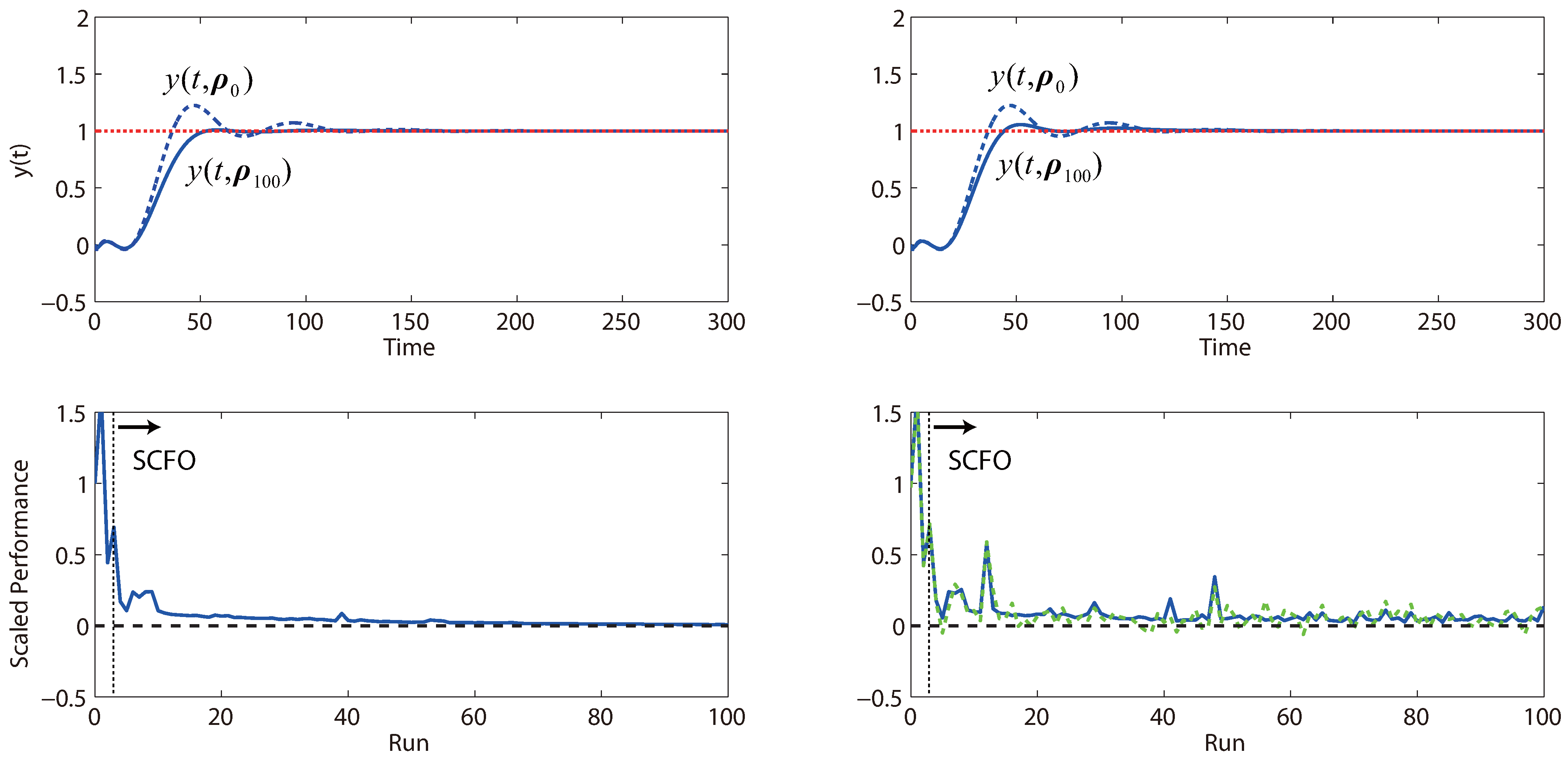
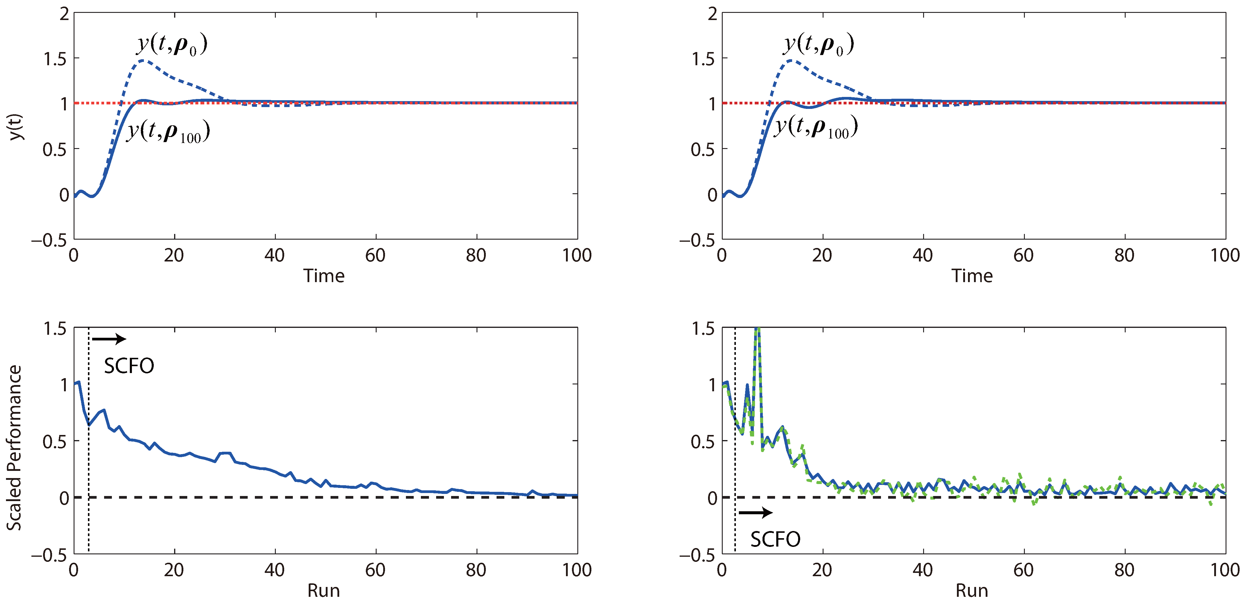
So as to study the effect of non-repeatability noise, each observed performance metric value is corrupted with an additive error from $\mathcal{N}(0,{(0.05J_0)}^2)$, i.e., by an additive error with a standard deviation that is chosen as 5% of the original performance metric value (assumed known for solver configuration). Noiseless scenarios were simulated as well.

Figure 13. Performance obtained by iterative tuning for both the noiseless (left) and noisy (right) cases of Study 1 of Problem (20), with the solid blue line used to denote the “true” performance of the closed-loop system and the green dashed line used to denote what is actually observed (and provided to the solver). In both cases, the SCFO solver brings the closed-loop performance metric value close to its global minimum of zero (marked by the black dashed line in the lower plots).

Figure 13. Performance obtained by iterative tuning for both the noiseless (left) and noisy (right) cases of Study 1 of Problem (20), with the solid blue line used to denote the “true” performance of the closed-loop system and the green dashed line used to denote what is actually observed (and provided to the solver). In both cases, the SCFO solver brings the closed-loop performance metric value close to its global minimum of zero (marked by the black dashed line in the lower plots).

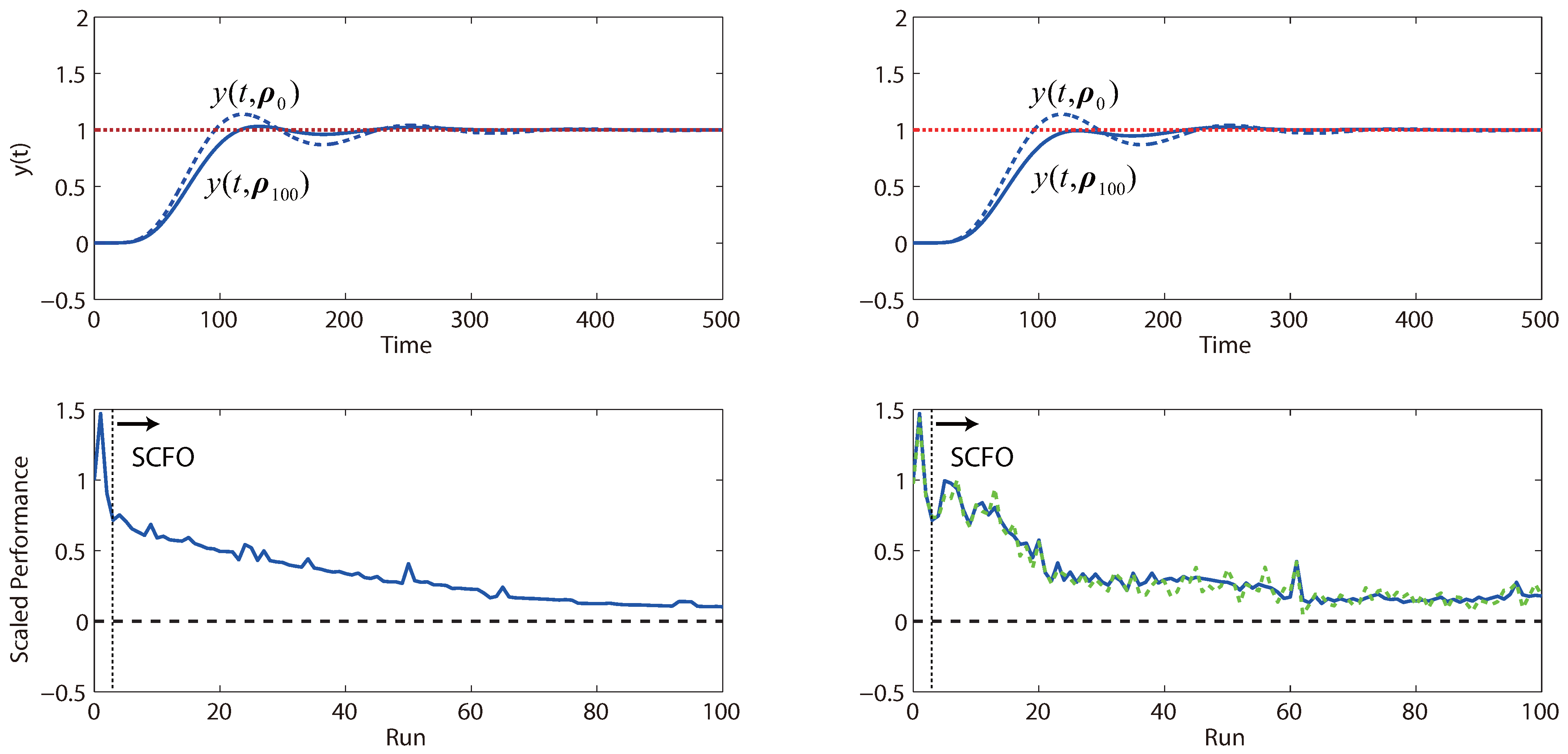
Figure 14. Performance obtained by iterative tuning for Study 2 of Problem (20).

Figure 14. Performance obtained by iterative tuning for Study 2 of Problem (20).

Figure 15. Performance obtained by iterative tuning for Study 3 of Problem (20).

Figure 15. Performance obtained by iterative tuning for Study 3 of Problem (20).

The results for the three studies are provided in Figure 13, Figure 14 and Figure 15. On the whole, we see that the solver reliably optimizes control performance in both the noiseless and noisy scenarios, even though we note that the rate of improvement can vary from problem to problem. For the noisy cases, we generally see more “bumps” in the convergence trajectory, which should not be surprising given (a) the added difficulty for the solver in estimating local derivatives and (b) the reduced conservatism in the estimation of the quadratic bound constants M, for which the safety factor η in Equation (16) is generally augmented less frequently when noise is present. However, for the latter point, we see that there is an upside with regard to convergence speed. Because the values of M tend to be less conservative in the presence of noise, the algorithm tends to take larger steps and progresses quicker towards the optimum, as is witnessed in both Figure 13 and Figure 15. We do note the occasional danger of performance worsening due to tuning, but this is almost always restricted to the earlier runs when the solver is relatively “data-starved”.

4.4. Tuning a System of PI Controllers for Setpoint Tracking and Disturbance Rejection

Here, we consider the following five-input, five-output dynamical system:

$$\begin{array}{ccc}\hfill {\ddot{y}}_1(t)+{\dot{y}}_1(t)+y_1(t)& =& u_1(t)-0.033u_3(t)-0.067u_4(t)-0.1u_5(t)\hfill \\ \hfill {\ddot{y}}_2(t)+0.1{\dot{y}}_2(t)+y_2(t)& =& 0.1u_1(t)+2u_2(t)+0.033u_3(t)-0.033u_5(t)\hfill \\ \hfill {\ddot{y}}_3(t)+5{\dot{y}}_3(t)+y_3(t)& =& 0.167u_1(t)+0.133u_2(t)+3u_3(t)+0.067u_4(t)+0.033u_5(t)\hfill \\ \hfill {\ddot{y}}_4(t)+2{\dot{y}}_4(t)+y_4(t)& =& 0.233u_1(t)+0.2u_2(t)+0.167u_3(t)+4u_4(t)+0.1u_5(t)\hfill \\ \hfill {\ddot{y}}_5(t)+3{\dot{y}}_5(t)+y_5(t)& =& 0.3u_1(t)+0.267u_2(t)+0.233u_3(t)+0.2u_4(t)+5u_5(t)\hfill \end{array}$$

(21)

While the user cannot be assumed to know the plant (21), we will assume that they have been able to properly decouple the system with the input-output pairings of $u_i\to y_i,i=1,...,5$ (as this is evidently the superior choice if one considers the relative gains). A system of five PI controllers is used for the pairings:

$$u_i(t)=K_{p,i}\left(e_i(t)+\frac{1}{{\tau }_{I,i}}{\int }_0^t{e}_i(t)dt\right),i=1,...,5$$

which, of course, is not perfect, since the decoupling is not either, and so what one controller does will inevitably affect the others.

The ICT problem that we define for this system consists of starting with all $y_i(0)=0$ and defining the setpoints of $y_1$, $y_3$ and $y_5$ as 1 (which makes this a tracking problem with respect to these outputs) and the setpoints of $y_2$ and $y_4$ as 0 (which makes it a disturbance rejection problem with respect to these two outputs). The total sum of squared tracking errors for all of the outputs is used as the performance metric, with the interval of $t\in [2,15]$ being considered in the metric computation (a “mask” of 2 time units being employed).

The first five tuning parameters are simply defined as the controller gains, with ${\rho }_i\stackrel{\Delta }{=}{K}_{p,i},i=1,...,5$. As in the previous example, we use a scaled version of the integral times to define the rest, with ${\rho }_{i+5}\stackrel{\Delta }{=}{\tau }_{I,i}/10,i=1,...,5$. Once again, as we do not know a priori what lower and upper limits should be set on these parameters (save the positivity of the ${\tau }_{I,i}$), adaptive inputs with the positivity limitation (as shown in the previous case study) are used.

Furthermore, we suppose the existence of a safety limitation in the form of a maximal value that $y_1$ is allowed to take, with the constraint $y_1(t)\le 1.2$ to be met at all times. Using the reformulation shown in Section 2.2, we may proceed to state this problem in RTO form as:

$$\begin{array}{cc}\hfill \underset{\mathit{\rho }}{\mathrm{minimize}}& {\displaystyle \frac{1}{J_0}\sum _{i=1}^5{\int }_2^{15}{\left[y_{i,ref}(t)-y_i(t,\mathit{\rho })\right]}^{2}dt}\hfill \\ \hfill \mathrm{subject}\mathrm{to}& y_{1,max}(\mathit{\rho })-1.2\le 0\hfill \\ & {\rho }_{k,1}-0.5\le {\rho }_1\le {\rho }_{k,1}+0.5\hfill \\ & {\rho }_{k,2}-0.5\le {\rho }_2\le {\rho }_{k,2}+0.5\hfill \\ & {\rho }_{k,3}-0.5\le {\rho }_3\le {\rho }_{k,3}+0.5\hfill \\ & {\rho }_{k,4}-0.5\le {\rho }_4\le {\rho }_{k,4}+0.5\hfill \\ & {\rho }_{k,5}-0.5\le {\rho }_5\le {\rho }_{k,5}+0.5\hfill \\ & max({\rho }_{k,6}-0.5,0.01)\le {\rho }_6\le {\rho }_{k,6}+0.5\hfill \\ & max({\rho }_{k,7}-0.5,0.01)\le {\rho }_7\le {\rho }_{k,7}+0.5\hfill \\ & max({\rho }_{k,8}-0.5,0.01)\le {\rho }_8\le {\rho }_{k,8}+0.5\hfill \\ & max({\rho }_{k,9}-0.5,0.01)\le {\rho }_9\le {\rho }_{k,9}+0.5\hfill \\ & max({\rho }_{k,10}-0.5,0.01)\le {\rho }_{10}\le {\rho }_{k,10}+0.5\hfill \end{array}\begin{array}{c}\left.\begin{array}{c}\hfill \\ \hfill \end{array}\right\}{\varphi }_p(\mathbf{v})\hfill \\ \left.\begin{array}{c}\hfill \end{array}\right\}{\mathbf{G}}_p(\mathbf{v})⪯\mathbf{0}\hfill \\ \left.\begin{array}{c}\hfill \\ \hfill \\ \hfill \\ \hfill \\ \hfill \\ \hfill \\ \hfill \\ \hfill \\ \hfill \\ \hfill \end{array}\right\}{\mathbf{v}}^L⪯\mathbf{v}⪯{\mathbf{v}}^U\hfill \end{array}$$

(22)

We note that this problem is a bit more challenging than the ones considered in the previous three studies due to the increased number of tuning parameters, and point out that, were the problem perfectly decoupled, we would be able to solve it as five two-parameter RTO problems in parallel. However, seeing as all of the parameters are intertwined, we have no choice but to optimize over all ten simultaneously—the expected price to pay being a slower rate of performance improvement obtained by the solver. Alternate strategies that are based on additional engineering knowledge, such as optimizing only the parameters of specific controllers or optimizing only the controller gains, could of course be proposed and are highly recommended.

As a somewhat arbitrary design, the initial set is chosen as ${\mathit{\rho }}_0:={\left[2222211111\right]}^T$. Like with the previous example, an additive measurement noise of $\mathcal{N}(0,{(0.05J_0)}^2)$ is added to corrupt the performance metric value that is observed for a given choice of tuning parameters. An additive measurement noise of $\mathcal{N}(0,{10}^{-4})$ is added to corrupt the observed values of $y_{1,max}$. Both sets of statistics are assumed to be known for the purposes of SCFO solver configuration. As before, the noiseless scenarios are also considered.

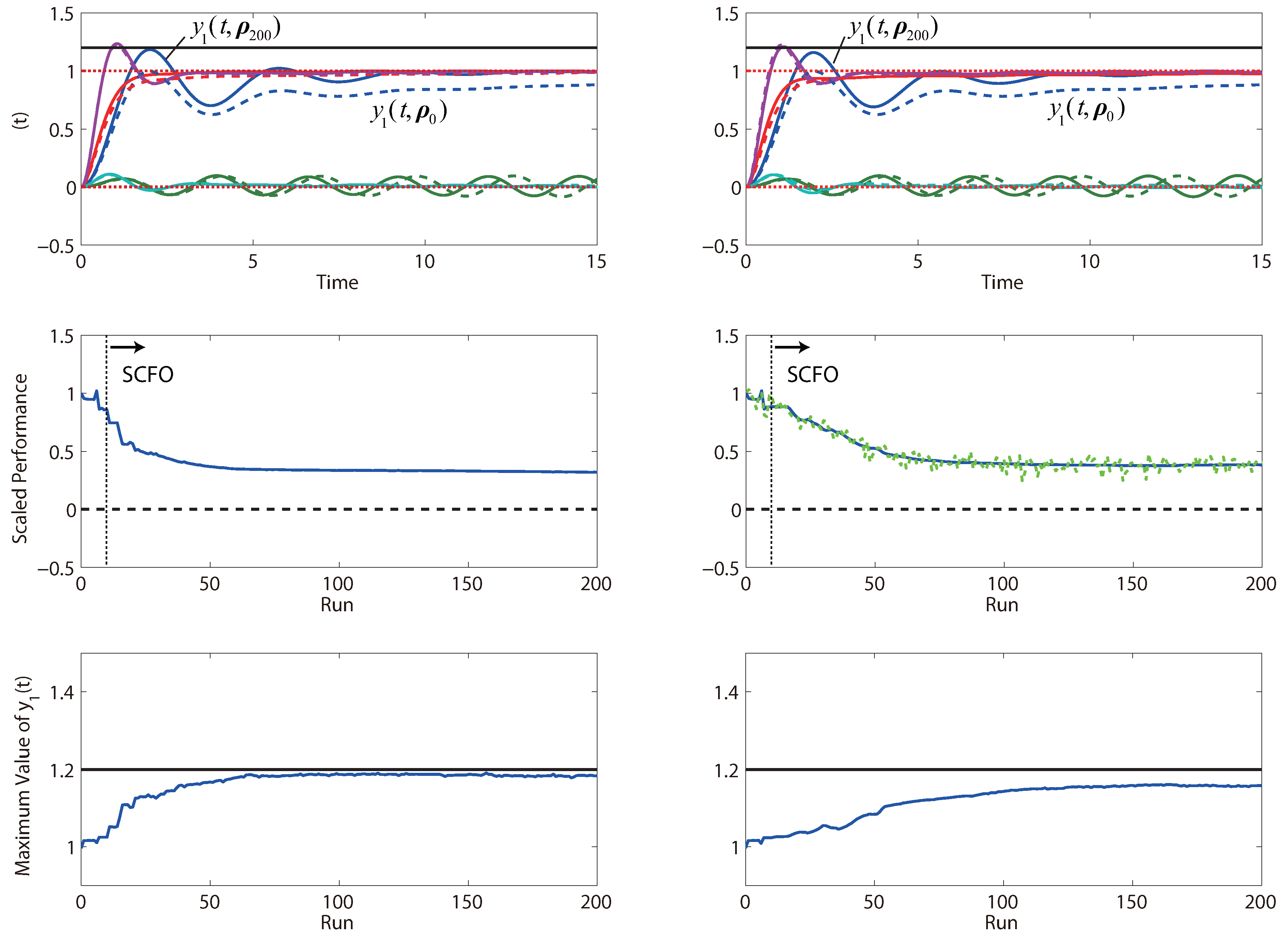
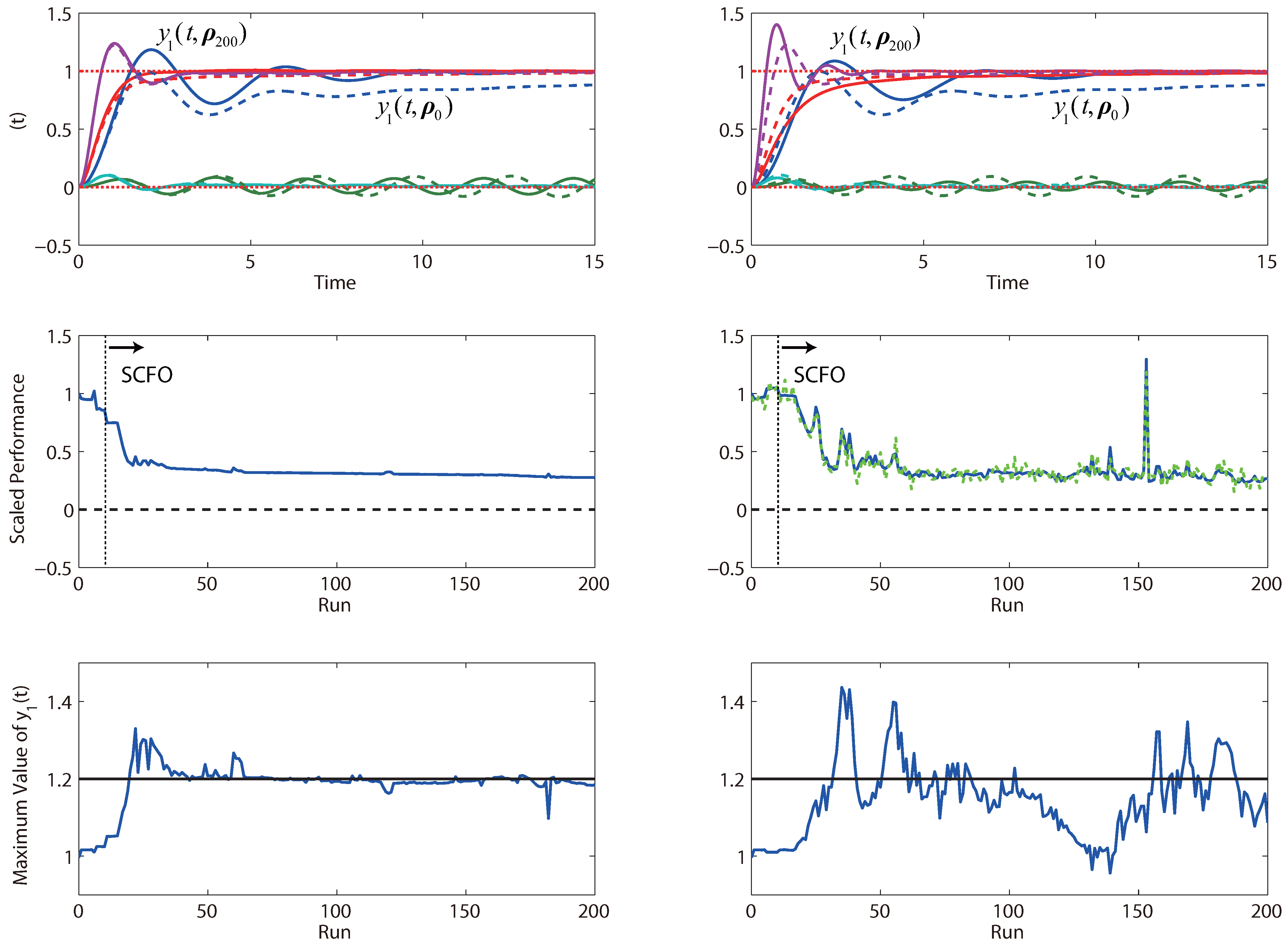
We present the results in Figure 16, which show that the solver is able to obtain significant performance improvements within 50 iterations for both the noiseless and noisy cases without once violating the output constraint on $y_1$. In this case, we see that the noise has the effect of slowing down convergence, which may be explained by the fact that the solver must take even more cautious steps so as not to violate the output constraint. Additionally, the performance that is observed after 200 iterations is a bit worse for the noisy case, which may be seen as being due to the back-off from the output constraint being larger (to account for the noise).

Figure 16. Performance obtained by iterative tuning for the system of PI controllers in Problem (22)—the noiseless case is given on the left and the noisy case on the right. For the output profiles, we note that the initial profiles are given as dashed lines, with the final profiles given by solid lines of the same color.

Figure 16. Performance obtained by iterative tuning for the system of PI controllers in Problem (22)—the noiseless case is given on the left and the noisy case on the right. For the output profiles, we note that the initial profiles are given as dashed lines, with the final profiles given by solid lines of the same color.

To test the effect of this constraint and to see if it is even necessary, we also run a simulation where the constraint is lifted from the problem statement. The results for this study are given in Figure 17 and show that not having the constraint in place certainly leads to runs where it is violated. This is not surprising, given that a lot of the performance improvement is obtained by tracking the setpoint of $y_1$ faster, which is easier to do once there is no constraint on its overshoot. It is also seen that the performance obtained after 200 iterations is generally better than what would be obtained with the constraint—this is, again, not surprising, as removing a limiting constraint should allow for greater performance gains. We do note that the noisy case is more bumpy without the constraint, which is expected, as there is less to limit the adaptation steps and more “daring” adaptations become possible. While some of the bumps may be quite undesired (particularly, the one noted just after the 150^th run), the algorithm remains, on the whole, reliable, as it keeps the performance metric at low values for the majority of the runs despite significant noise corruption.

Figure 17. Performance obtained by iterative tuning for the system of PI controllers in Problem (22) (without an output constraint).

Figure 17. Performance obtained by iterative tuning for the system of PI controllers in Problem (22) (without an output constraint).

5. Concluding Remarks

The goal of this paper has been to propose the idea of posing the iterative controller tuning (ICT) problem in the real-time optimization (RTO) framework, and it has been shown how one can easily formulate most ICT problems as RTO ones with the use of a repeatability assumption that, though only an approximation of reality in the presence of noise, disturbances, or degradation, appears to suffice for application purposes (at least, in the two experimental case studies considered here). A major advantage of this reformulation is that a number of previously unaddressed challenges in ICT, the majority of which take the form of constraints in the performance metric minimization problem, may be addressed in a fairly straightforward manner. To make the message more concrete, we have also shown how the ICT problem may be solved by the SCFO real-time optimization solver and have provided the reader with the necessary solver settings to do so. Four case studies have shown the method to work very well for a diverse range of problems.

Though we hope to have convinced the reader that the method proposed makes for a strong candidate for solving general ICT problems in practice, its potential drawbacks should be clear:

• No solution has been proposed for how to treat the case where the repeatability assumption is not a good approximation of reality. Instead of hoping that the approximation suffices in practice, it would be beneficial to propose alternatives that would still allow one to use the RTO framework to deal with the problem. In particular, one could attempt to make the repeatability assumption on the input and output trajectories rather than making it directly on the performance metric. This could allow one to establish a closer link between the lack of repeatability and the input/output noise in the control system.
• Although the proposed configuration has been shown to be largely successful here, many of the elements involved still remain heuristic in nature. Either improving on these heuristics or finding ways to avoid them are desired.
• The method is currently limited to solving ICT problems where the control task remains the same, which may significantly limit its domain of applicability. It would be interesting to attempt to extend it to cases where the control tasks were similar, rather than identical, and then somehow penalize the method based on the degree of similarity (e.g., one could attempt to lump non-similarity into the noise element δ of the repeatability assumption).

We finish by noting that an abstract advantage of the RTO-ICT formulation is that we are now able to attack the ICT problem from two directions—that of control and that of RTO. For the former, we note that the proposed method applies very few control principles (unlike other direct tuning methods [9,10], which make heavy use of control theory). While this is, in some sense, an advantage—as it allows us to use the proposed method to tune almost any controller for almost any system—there is undoubtedly something lost due to the “black-box veil” that the RTO formulation places on the problem, and incorporating additional knowledge for specific controllers would very likely allow for further improvements to the techniques discussed here. At the same time, the RTO methods themselves are in a fairly nascent stage theoretically. Many improvements to both RTO theory and solution methods are expected to appear in the coming years, which could only improve on the results presented here and make the solution of the ICT problem both faster and more reliable.