An MINLP Model that Includes the Effect of Temperature and Composition on Property Balances for Mass Integration Networks

Abstract
:1. Introduction
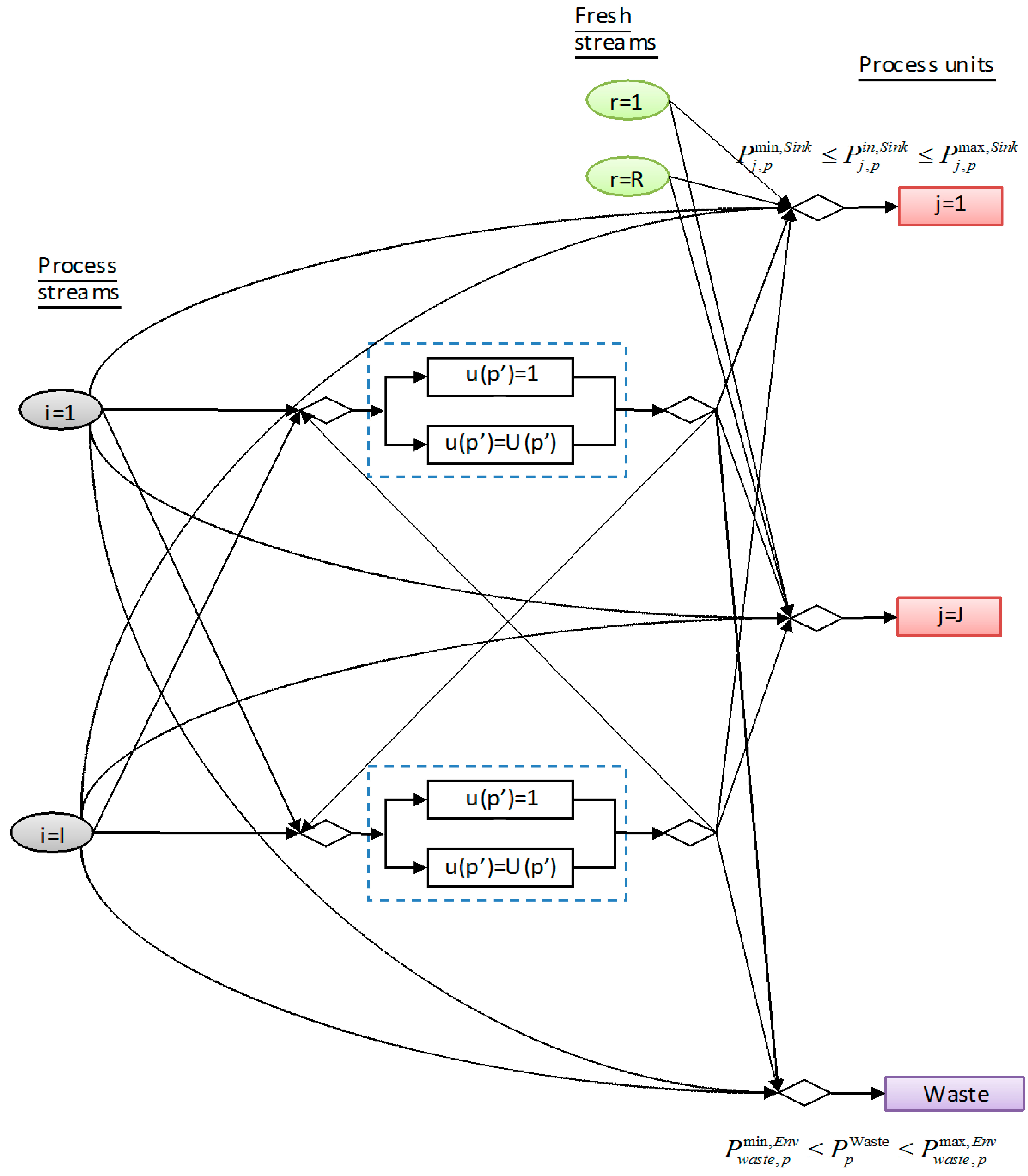
2. Problem Statement
3. Model Formulation

3.1. Splitting of Process Streams
3.2. Splitting of Fresh Streams
3.3. Mass Balance at Inlet of Process Interceptors
3.4. Property Balance at Inlet of Property Interceptors

| Property | Operator |
|---|---|
| Composition | ψz(z) = z |
| Toxicity | ψTox(Tox) = Tox |
| Chemical Oxygen Demand | ψCOD(COD) = COD |
| pH | ψpH(pH) = 10pH |
| Density | |
| Viscosity | ψμ(μ) = log (μ) |
3.5. Energy Balances at the Inlet of Property Interceptors
3.6. Property Interceptors
3.7. Stream Splitting at the Outlet of Each Property Interceptor
3.8. Mass Balance for Process Sinks
3.9. Property Balance for Process Sinks
3.10. Energy Balance for Process Sinks
3.11. Mass Balance for Waste Stream
3.12. Property Balance in Waste Stream
3.13. Energy Balance in Waste Stream
3.14. Constraints
3.15. Modification of Properties
3.16. Properties as a Function of Temperature
4. Methodology for Estimation of Parameters
- (1)
- From the set of data, Equation (31) is used to obtain the parameter values. Temperature, , concentration ψZ(PX) and the uncorrected property operator are independent variables.
- (2)
- To estimate the parameters, takes the value for the property operator p(T) for the original process streams.
- (3)
- With the calculated parameters, the equation is implemented into the MINLP model.
4.1. Viscosity
4.2. Density
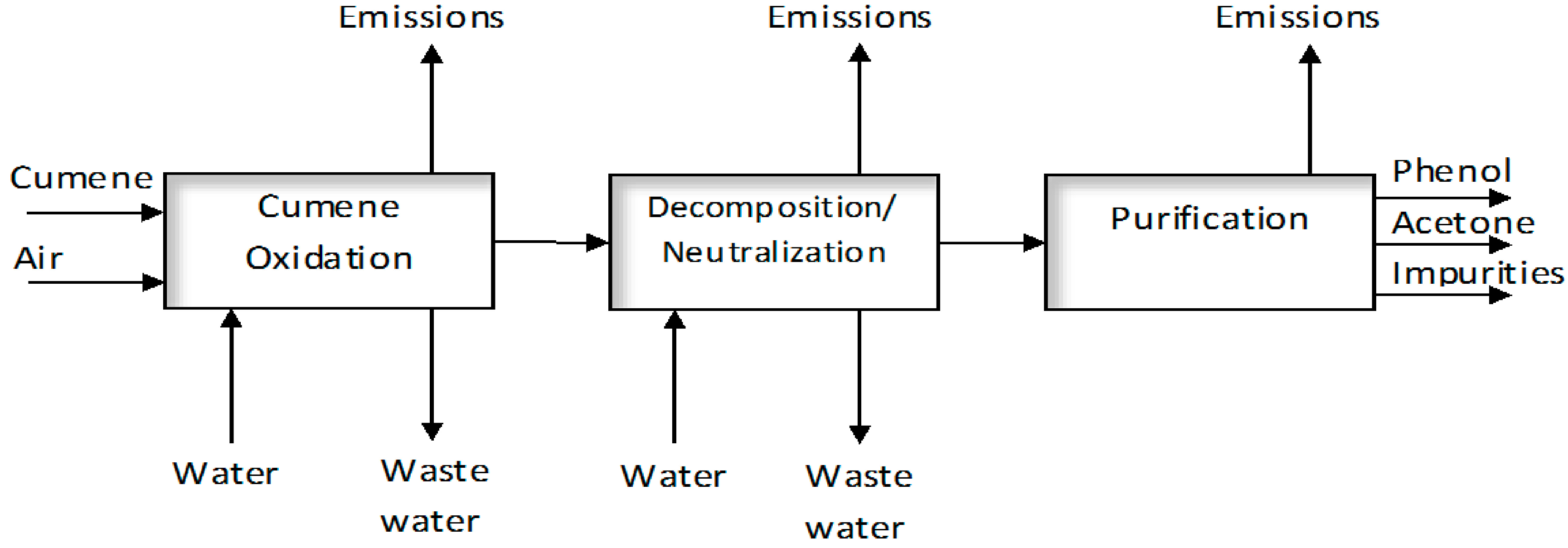
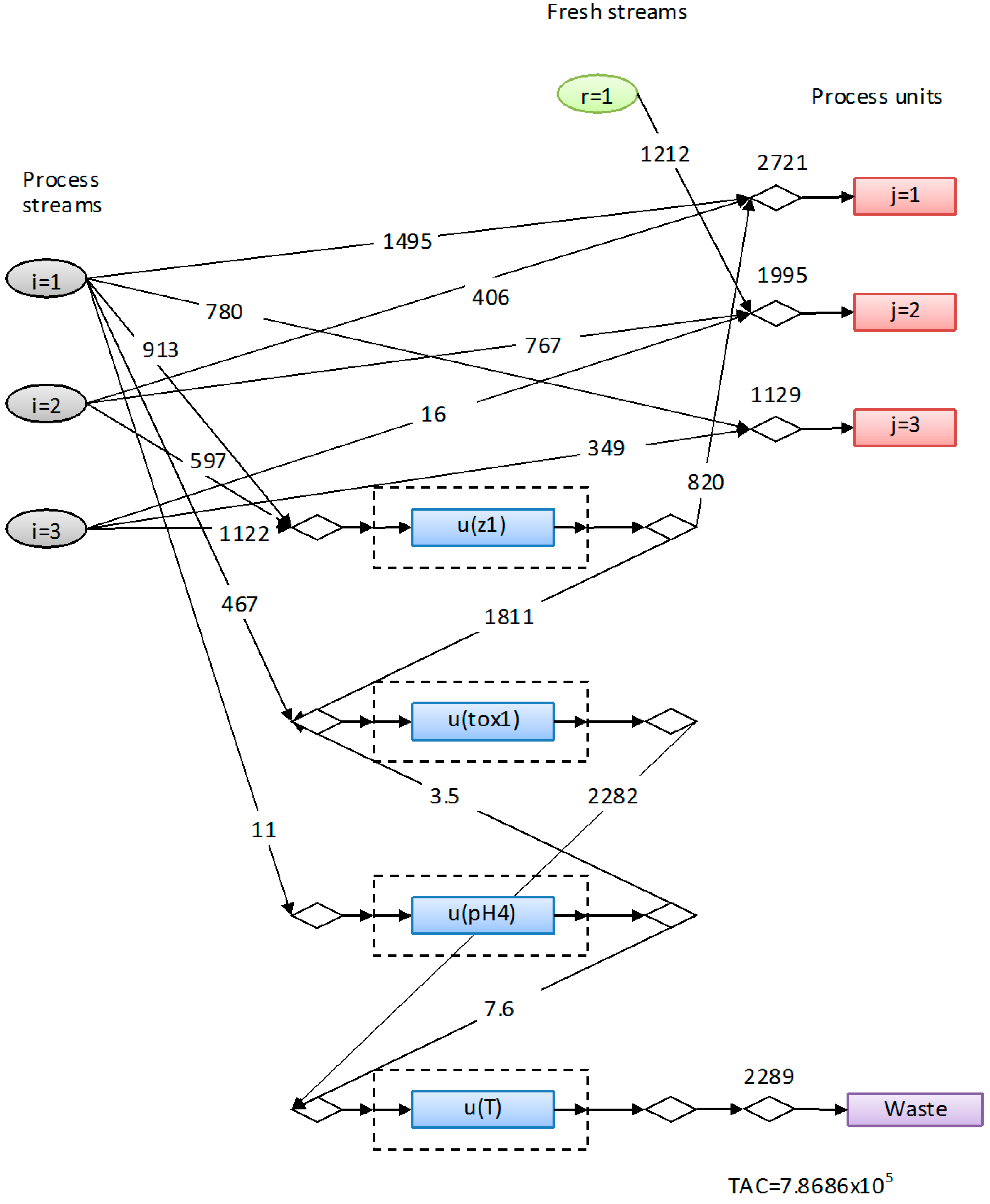
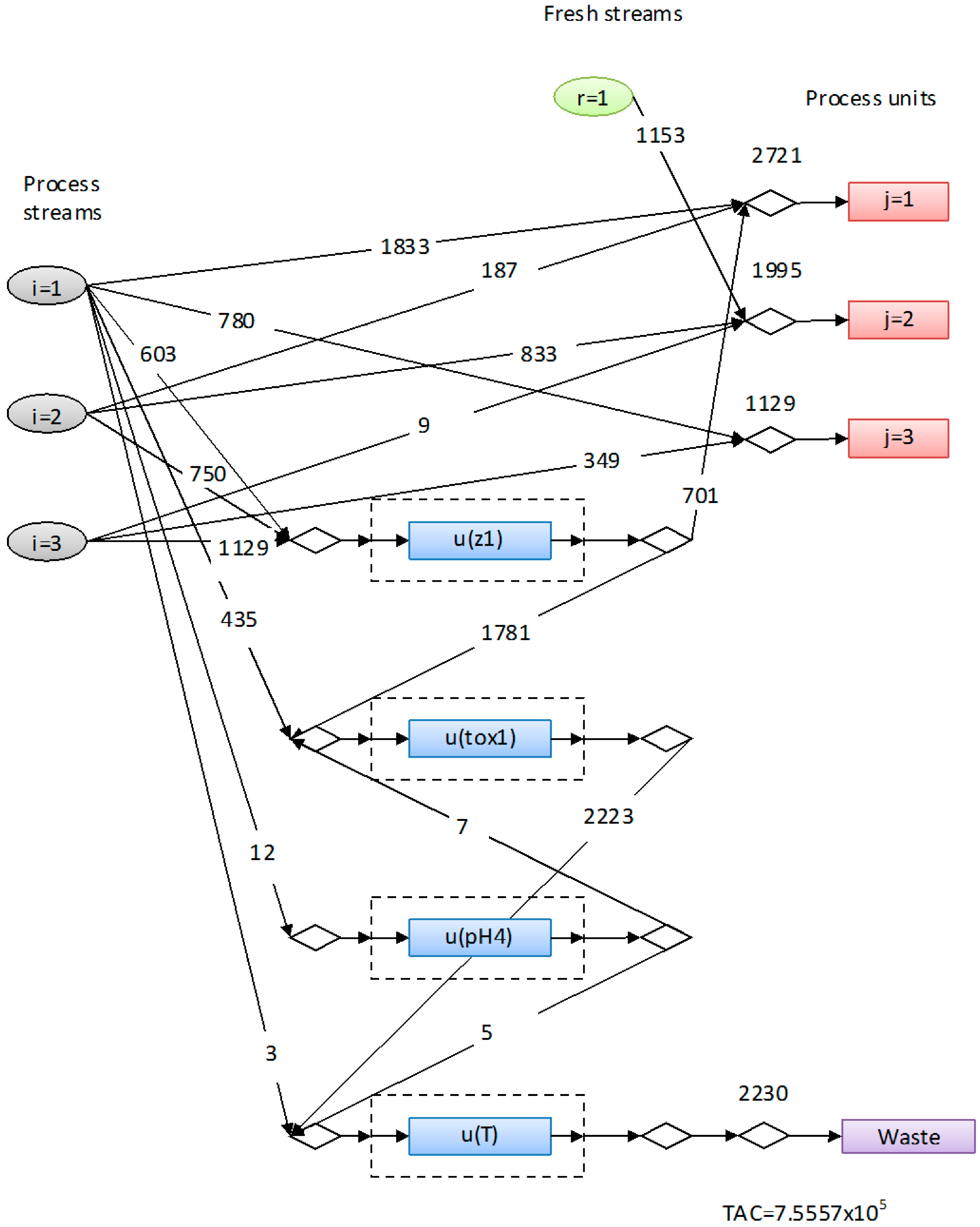
5. Case Study

| Stream | Flow (kg/h) | Z | Tox (%) | COD (mgO2/L) | pH | ρ* (kg/m3) | µ* (cP) | T (K) | Cp** (kJ/kg K) |
|---|---|---|---|---|---|---|---|---|---|
| R1 | - | 0 | 0 | 0 | 7.0 | 994.0 | 0.913 | 298.15 | 4.1845 |
| R2 | - | 0.010 | 0.1 | 0.010 | 7.1 | 986.1 | 0.743 | 308.15 | 4.1575 |
| W1 | 3666 | 0.016 | 0.3 | 0.187 | 5.4 | 947.1 | 0.382 | 348.15 | 4.1601 |
| W2 | 1769 | 0.024 | 0.5 | 48.450 | 5.1 | 958.8 | 0.442 | 338.15 | 4.1363 |
| W3 | 1487 | 0.220 | 1.5 | 92.100 | 4.8 | 1022.1 | 0.745 | 313.15 | 3.7280 |
| Stream | Flow (kg/h) | Zmax | Toxmax (%) | CODmax (mgO2/L) | pH max | ρmax (kg/m3) | µmax (cP) |
|---|---|---|---|---|---|---|---|
| G1 | 2721 | 0.013 | 2 | 100 | 8.0 | 1270 | 1.202 |
| G2 | 1995 | 0.011 | 2 | 100 | 7.8 | 1113 | 2.230 |
| G3 | 1129 | 0.100 | 2 | 100 | 8.2 | 1315 | 1.260 |
| Waste | - | 0.005 | 0.001 | 75 | 9.0 | - | - |
| Sink/Waste | Flow (kg/h) | pHmin | ρmin (kg/m3) | µmin (cP) |
|---|---|---|---|---|
| G1 | 2721 | 5.3 | 816 | 0.2 |
| G2 | 1995 | 5.4 | 771 | 0.2 |
| G3 | 1129 | 5.2 | 839 | 0.2 |
| Waste | - | 5.5 | - | - |
| Sink/Waste | Tmin (K) | Tmax (K) |
|---|---|---|
| G1 | 333.15 | 353.15 |
| G2 | 303.15 | 348.15 |
| G3 | 298.15 | 338.15 |
| Waste | 290.15 | 308.15 |
| Property | αu,m | ($/kg) |
|---|---|---|
| u(z1) | 0.98 | 0.0143 |
| u(z2) | 0.85 | 0.0073 |
| u(Tox1) | 1.00 | 0.0216 |
| u(Tox2) | 0.90 | 0.0165 |
| u(COD1) | 0.80 | 0.0143 |
| u(COD2) | 0.55 | 0.0071 |
| u(pH1) | 0.50 | 0.1389 |
| u(pH2) | 0.30 | 0.0397 |
| u(pH3) | −0.50 | 0.1433 |
| u(pH4) | −0.30 | 0.0419 |
| Compound | Ac | Bc | Cc |
|---|---|---|---|
| Water | 5.8221 | −0.01033 | 0.0000162 |
| Phenol | 1.0809 | 0.003375 | 0 |
| p(T) | C1,p(T) | C2,p(T) | C3,p(T) | C4,p(T) |
|---|---|---|---|---|
| Viscosity | −2.6816 | 786.50 | 0.18400 | −2.0699 × 10⁻⁵ |
| Density | 6.8632 × 10⁻⁴ | 1.0715 × 10⁻⁶ | −1.9655 × 10⁻⁴ | −3.9471 × 10⁻⁴ |

| Z | Tox (%) | COD (mgO2/L) | pH | ρ (kg/m3) | µ (cP) | T (K) | |
|---|---|---|---|---|---|---|---|
| G1 | 0.013 | 0.4978 | 22.549 | 5.30 | 953.3 | 0.4220 | 341.28 |
| G2 | 0.011 | 0.2043 | 19.515 | 6.79 | 980.7 | 0.6740 | 313.57 |
| G3 | 0.079 | 0.6707 | 28.577 | 5.29 | 968.3 | 0.4558 | 338.15 |
| Waste | 0.005 | 0.0010 | 39.828 | 5.50 | 985.1 | 0.7441 | 308.15 |

| Source | G1 | G2 | G3 | Waste |
|---|---|---|---|---|
| Aspen | 953.64 | 981.01 | 968.81 | 985.20 |
| Model with p(z,T) | 953.29 | 980.68 | 968.34 | 985.12 |
| Error, % | 0.04 | 0.033 | 0.049 | 0.01 |
| Model, no p(z,T) | 958.72 | 980.36 | 969.10 | 956.22 |
| Error, % | 0.53 | 0.07 | 0.03 | 2.94 |
| Source | G1 | G2 | G3 | Waste |
|---|---|---|---|---|
| Aspen | 0.4208 | 0.6686 | 0.4506 | 0.7414 |
| Model with p(T) | 0.4220 | 0.6740 | 0.4558 | 0.7441 |
| Error, % | 0.29 | 0.80 | 1.17 | 0.37 |
| Model, no p(T) | 0.4297 | 0.6898 | 0.4694 | 0.4526 |
| Error, % | 2.12 | 3.17 | 4.18 | 38.95 |
6. Conclusions
Acknowledgments
Author Contributions
Nomenclature
| A,B,C | empirical parameters |
| COD | chemical oxygen demand |
| CostFresh | cost of fresh sources |
| CostInt | cost of property interceptor |
| CP | heat capacity |
| d | stream flowrate |
| F, f | flowrate of fresh sources |
| G, g | flowrate of process sinks |
| HV | operating hours per year |
| p, p' | any property |
| q | flowrate from interceptors |
| R, r | Flowrate of fresh sources |
| sink | process sink |
| source | fresh or stream source |
| T | temperature |
| TAC | total annual cost |
| Tox | toxicity |
| x | mole fraction |
| W, w | flowrate of process streams |
| waste | waste discharged to the environment |
| Y | Boolean variable |
| y | binary variable |
| z | pollutant concentration |
Sets
| I | process streams |
| J | sinks |
| M | properties to be treated |
| R | fresh sources |
| Up | treatment units for each property |
Subindices
| i | process stream |
| j | sink |
| r | fresh source |
Superscripts
| C | corrected |
| In | inlet |
| Int | interceptor |
| max | maximum |
| min | minimum |
| Out | outlet |
| UnC | uncorrected |
Greek symbols
| α | separation efficiency of property interceptor |
| Ψ | property operator |
| ρ | density |
| μ | viscosity |
Conflicts of Interest
References
- Hohmann, E.C. Optimum Networks for Heat Exchange. Ph.D. Thesis, University of Southern California, Los Angeles, CA, USA, 1971. [Google Scholar]
- Linnhoff, B.; Flower, J.R. Synthesis of heat exchanger networks: I. Systematic generation of energy optimal networks. AIChE J. 1978, 24, 633–642. [Google Scholar]
- Umeda, T.; Itoh, J.; Shiroko, K. Heat-exchanger system synthesis. Chem. Eng. Prog. 1978, 74, 70–76. [Google Scholar]
- El-Halwagi, M.M.; Manousiouthakis, V. Synthesis of mass exchange networks. AIChE J. 1989, 35, 1233–1244. [Google Scholar]
- Wang, Y.P.; Smith, R. Wastewater minimization. Chem. Eng. Sci. 1994, 49, 981–1006. [Google Scholar] [CrossRef]
- Dhole, V.R.; Ramchandani, N.; Tainsh, R.A.; Wasilewski, M. Make your process Water pay for itself. Chem. Eng. 1996, 103, 100–103. [Google Scholar]
- El-Halwagi, M.M.; Hamad, A.A.; Garrison,, G.W. Synthesis of waste interception and allocation networks. AIChE J. 1996, 42, 3087–3101. [Google Scholar]
- El-Halwagi, M.M.; Spriggs, H.D. Solve design puzzles with mass integration. Chem. Eng. Prog. 1998, 94, 25–44. [Google Scholar]
- Polley, G.T.; Polley, H.L. Design better water reuse networks. Chem. Eng. Prog. 2000, 96, 47–52. [Google Scholar]
- Foo, D.C.Y. State-of-the-art review of pinch analysis techniques for water network synthesis. Ind. Eng. Chem. Res. 2009, 48, 5125–5159. [Google Scholar] [CrossRef]
- Galan, B.; Grossmann, I.E. Optimal design of distributed wastewater treatment networks. Ind. Eng. Chem. Res. 1998, 37, 4036–4048. [Google Scholar] [CrossRef]
- Lee, S.; Grossmann, I.E. Global optimization of nonlinear generalized disjunctive programming with bilinear equality constraints: Applications to process networks. Comput. Chem. Eng. 2003, 27, 1557–1575. [Google Scholar] [CrossRef]
- Karuppiah, R.; Grossmann, I.E. Global optimization for the synthesis of integrated water systems in chemical processes. Comput. Chem. Eng. 2006, 20, 650–673. [Google Scholar] [CrossRef]
- Savelski, M.J.; Bagajewicz, M.J. On the optimality conditions of water utilization systems in process plants with single contaminants. Chem. Eng. Sci. 2000, 55, 5035–5048. [Google Scholar] [CrossRef]
- Savelski, M.J.; Bagajewicz, M.J. Algorithmic procedure to design water utilization systems featuring a single contaminant in process plants. Chem. Eng. Sci. 2001, 56, 1897–1911. [Google Scholar] [CrossRef]
- Tan, R.R.; Ng, D.K.S.; Foo, D.C.Y.; Aviso, K.B. A superstructure model for the synthesis of single-contaminant water networks with partitioning regenerators. Process Saf. Environ. Prot. 2009, 87, 197–205. [Google Scholar] [CrossRef]
- Teles, J.; Castro, P.M.; Novals, A.Q. LP-based solution strategies for the optimal design of industrial water networks with multiple contaminants. Chem. Eng. Sci. 2008, 63, 376–394. [Google Scholar] [CrossRef]
- Shelley, M.D.; El-Halwagi, M.M. Component-less design of recovery and allocation systems: A functionality-based clustering approach. Comput. Chem. Eng. 2000, 24, 2081–2091. [Google Scholar] [CrossRef]
- Qin, X.; Gabriel, F.; Harell, D.; El-Halwagi, M. Algebraic techniques for property integration via componentless design. Ind. Eng. Chem. Res. 2004, 43, 3792–3798. [Google Scholar] [CrossRef]
- El-Halwagi, M.M.; Glasgow, I.M.; Qin, X.Y.; Eden, M.R. Property integration: Componentless design techniques and visualization tools. AIChE J. 2004, 50, 1854–1869. [Google Scholar]
- Eljack, F.T.; Abdelhady, A.F.; Eden, M.R.; Gabriel, F.; Qin, X.; El-Halwagi, M.M. Targeting optimum resource allocation using reverse problem formulations and property clustering techniques. Comput. Chem. Eng. 2005, 29, 2304–2317. [Google Scholar] [CrossRef]
- Eljack, F.; Eden, M.; Kazantzi, V.; Qin, X.; El-Halwagi, M.M. Simultaneous process and molecular design—A property based approach. AIChE J. 2007, 53, 1232–1239. [Google Scholar] [CrossRef]
- Foo, D.C.Y.; Kazantzi, V.; El-Halwagi, M.M.; Manan, A. Surplus diagram and cascade analysis techniques for targeting property-based material reuse network. Chem. Eng. Sci. 2006, 61, 2626–2642. [Google Scholar] [CrossRef]
- Ponce-Ortega, J.M.; Hortua, A.C.; El-Halwagi, M.M.; Jiménez-Gutiérrez, A. A property-based optimization of direct recycle networks and wastewater treatment processes. AIChE J. 2009, 55, 2329–2344. [Google Scholar]
- Ponce-Ortega, J.M.; El-Halwagi, M.M.; Jiménez-Gutiérrez, A. Global optimization for the synthesis of property-based recycle and reuse networks including environmental constraints. Comput. Chem. Eng. 2010, 34, 318–330. [Google Scholar]
- Ponce-Ortega, J.M.; Nápoles-Rivera, F.; El-Halwagi, M.M.; Jiménez-Gutierrez, A. An optimization approach for the synthesis of recycle and reuse water integration networks. Clean Technol. Environ. Policy 2012, 14, 133–151. [Google Scholar]
- Nápoles-Rivera, F.; Ponce-Ortega, J.M.; El-Halwagi, M.M.; Jiménez-Gutiérrez, A. Global optimization of mass and property integration networks with in-plant property interceptors. Chem. Eng. Sci. 2010, 65, 4363–4377. [Google Scholar]
- Nápoles-Rivera, F.; Ponce-Ortega, J.M.; El-Halwagi, M.M.; Jiménez-Gutiérrez, A. Global optimization of wastewater integration networks for processes with multiple contaminants. Environ. Prog. Sustain. Energy 2012, 31, 449–458. [Google Scholar]
- El-Halwagi, M.M. Pollution Prevention through Process Integration: Systematic Design Tools; Elsevier Academic Press: San Diego, CA, USA, 1997. [Google Scholar]
- El-Halwagi, M.M. Process Integration; Elsevier Academic Press: San Diego, CA, USA, 2006. [Google Scholar]
- El-Halwagi, M.M. Sustainable Design through Process Integration: Fundamentals and Applications to Industrial Pollution Prevention, Resource Conservation, and Profitability Enhancement; Butterworth-Heinemann/Elsevier: Amsterdam, The Netherlands, 2012. [Google Scholar]
- Duhne, C.R. Viscosity-temperature correlations for liquids. Chem. Eng. 1979, 86, 83–91. [Google Scholar]
- Kheireddine, H.; Dadmohammadi, Y.; Deng, C.; Feng, X.; El-Halwagi, M.M. Optimization of direct recycle networks with the simultaneous consideration of property, mass, and thermal effects. Ind. Eng. Chem. Res. 2011, 50, 3754–3762. [Google Scholar] [CrossRef]
© 2014 by the authors; licensee MDPI, Basel, Switzerland. This article is an open access article distributed under the terms and conditions of the Creative Commons Attribution license (http://creativecommons.org/licenses/by/3.0/).
Share and Cite
Jiménez-Gutiérrez, A.; Sandate-Trejo, M.D.C.; El-Halwagi, M.M. An MINLP Model that Includes the Effect of Temperature and Composition on Property Balances for Mass Integration Networks. Processes 2014, 2, 675-693. https://doi.org/10.3390/pr2030675
Jiménez-Gutiérrez A, Sandate-Trejo MDC, El-Halwagi MM. An MINLP Model that Includes the Effect of Temperature and Composition on Property Balances for Mass Integration Networks. Processes. 2014; 2(3):675-693. https://doi.org/10.3390/pr2030675
Chicago/Turabian StyleJiménez-Gutiérrez, Arturo, María Del Carmen Sandate-Trejo, and Mahmoud M. El-Halwagi. 2014. "An MINLP Model that Includes the Effect of Temperature and Composition on Property Balances for Mass Integration Networks" Processes 2, no. 3: 675-693. https://doi.org/10.3390/pr2030675