Article

Parallel Solution of Robust Nonlinear Model Predictive Control Problems in Batch Crystallization

1
School of Chemical Engineering, Purdue University, 480 Stadium Mall Drive, West Lafayette, IN 47907, USA
2
Department of Chemical Engineering, Texas A&M University, 3122 TAMU, College Station, TX 77843, USA
*
Author to whom correspondence should be addressed.
Processes 2016, 4(3), 20; https://doi.org/10.3390/pr4030020
Submission received: 6 May 2016 / Revised: 20 June 2016 / Accepted: 22 June 2016 / Published: 30 June 2016
(This article belongs to the Special Issue Algorithms and Applications in Dynamic Optimization)

Abstract

:
Representing the uncertainties with a set of scenarios, the optimization problem resulting from a robust nonlinear model predictive control (NMPC) strategy at each sampling instance can be viewed as a large-scale stochastic program. This paper solves these optimization problems using the parallel Schur complement method developed to solve stochastic programs on distributed and shared memory machines. The control strategy is illustrated with a case study of a multidimensional unseeded batch crystallization process. For this application, a robust NMPC based on min–max optimization guarantees satisfaction of all state and input constraints for a set of uncertainty realizations, and also provides better robust performance compared with open-loop optimal control, nominal NMPC, and robust NMPC minimizing the expected performance at each sampling instance. The performance of robust NMPC can be improved by generating optimization scenarios using Bayesian inference. With the efficient parallel solver, the solution time of one optimization problem is reduced from 6.7 min to 0.5 min, allowing for real-time application.

Graphical Abstract

1. Introduction

Nonlinear model predictive control (NMPC) is an advanced control technique based on an online solution of a nonlinear optimal control problem at each sampling instance using new measurements and updated state estimates. The quality of NMPC depends on the accuracy of the underlying model. Despite the high fidelity of using nonlinear models based on first principles, there are still uncertainties associated with external and internal disturbances. Although the inherent robust Input-to-State Stability (ISS) of NMPC can be proven for ideal NMPC [1,2], the assumption that the existence of uncertainties do not change the feasibility (e.g., no state and input constraints) is not valid for many applications. Even if robust stability is valid, it is of limited use in analyzing the robust performance, especially for batch processes.
Several approaches have been proposed to take uncertainty into consideration in the design of NMPC algorithms. The most widely-studied approach is to solve a min–max optimization at each sampling instance to minimize the performance index of the worst-case while satisfying the state and input constraints for a set of uncertainty realizations [3]. One concern about this approach is that the nominal performance is sacrificed as the min–max optimization often chooses a very conservative control strategy. Huang et al. [4] proposes to minimize the expected value of the performance index based on multiple uncertainty scenarios. Nagy and Braatz [5] minimizes a weighted sum of expected value and variance of the performance index. While all of these approaches can be implemented within a feedback framework, this feedback is not considered in the NMPC optimization formulation itself. By contrast, Magni et al. [6] optimizes the control laws instead of the control steps at each sampling step. However, if the form of the control law is overly complex, this approach may not be computationally feasible. Recently, several other methods including multi-stage NMPC [7], Riccati differential equations [8] and a relaxation-based approach [9] were reported.
If we represent the uncertainties with a set of scenarios, the multi-scenario-based robust NMPC problem can be viewed as a large-scale stochastic program. The problem size becomes too large to be solved efficiently online by a serial solver, driving the need for parallel algorithms. For stochastic programs, an efficient parallel algorithm often exploits the structure at problem formulation level (e.g., Bender decomposition, Lagrangian decomposition, Lagrangian relaxation, progressive hedging) or at linear algebra level. Although the parallelization of the first class can be easily implemented, the convergence rate is typically slow, especially for nonlinear problems. In contrast, the second class of approaches can retain the fast convergence properties of the original host algorithms. For this class, interior-point methods are popular because the structure of the linear system remains the same at each iteration. The linear systems derived using interior-point methods for stochastic programming problems have the block-bordered-diagonal form, and they can be decomposed using the Schur complement method [10]. When the number of first stage variables is small, this approach has almost perfect strong scaling. However, when the number of first stage variables is large, forming and solving the dense Schur complement becomes a computational bottleneck.
In order to deal with stochastic programs with large first-stage dimensionality, many approaches have been proposed. Kang et al. [11] uses a preconditioned conjugate gradient (PCG) procedure to solve the Schur system with an automatic L-BFGS preconditioner. This approach avoids both forming and factorizing the Schur complement explicitly. Lubin et al. [12] forms the Schur system as a by-product of a sparse factorization and factorizes the Schur system in parallel. Cao et al. [13] performs adaptive clustering of scenarios inside-the-solver and forms a sparse compressed representation of the large Karush–Kuhn–Tucker(KKT) system as a preconditioner. The matrix that needs to be factorized in this approach is much smaller than the full-space KKT system and more sparse than the Schur system.
In addition to the parallel solution of the KKT system, a scalable parallel algorithm also requires parallel evaluations of the nonlinear programming (NLP) functions and gradients, and parallel implementations of all other linear algebra operations (e.g., vector-vector operations and matrix-vector multiplications). While the latter is easy for many parallel architectures, the former is not. There is, to the best knowledge of the author, no efficient modeling language supporting parallel evaluations of functions and gradients for general NLP problems. However, for structured problems such as stochastic programs, Kang et al. [11] and Zavala et al. [10] build a single AMPL [14] model instance for each scenario and evaluate all these instances in parallel. Several packages (e.g., PySP [15], StochJuMP [16]) have also been developed to support the parallel evaluation of functions and gradients for structured NLP problems.
This paper solves optimization problems arising from robust NMPC using the parallel algorithm developed to solve stochastic programs. This paper is organized as follows: Section 2 presents both the NMPC and robust NMPC approaches. Section 3 describes one parallel algorithm to solve large-scale stochastic programs based on the Schur complement method. Section 4 illustrates this approach with a case study of a batch crystallization process, and compares the performance of robust NMPC with open-loop control and nominal NMPC. Final conclusions are presented in Section 5.

2. Problem Formulations

This section demonstrates the problem formulations in the context of batch processes, while the solution strategy described in Section 3 can also be applied to continuous processes.

2.1. NMPC Formulation

For a batch process in the interval [ t 0 , t f ], the optimal control problem solved online at a sampling instance t k is of the following form:
min u ( t ) J ( z ( t ) , u ( t ) , p ) ,
s . t . d z ( t ) d t = f ( z ( t ) , u ( t ) , p ) ,
y ( t ) = c ( z ( t ) , u ( t ) , p ) ,
z ( t k ) = z ^ ( t k ) ,
g ( z ( t ) , u ( t ) , p ) 0 , t [ t k , t f ] ,
where J is the objective function, t is the time, z ( t ) is the vector of n z state variables, u denotes the vector of n u input variables, p represents the vector of n p uncertainty parameters, and y ( t ) is the vector of n y output variables. The initial state values z ^ ( t k ) of the process are estimated using moving horizon estimation (MHE) from the historical measurement of y ( t ) , t [ t 0 , t k ] . The function f describes the system dynamics and the function g represents the constraints on the inputs and state variables. After solving the above optimal control problem, the input trajectory in the interval [ t k , t k + 1 ) is injected in the plant. The optimization process is repeated with the updated estimation of z ^ ( t k + 1 ) at the next sampling instance t k + 1 .
For batch processes, the objective function usually only depends on the product quality at the end of the process. Therefore, one popular expression of the objective function is:
y ( t f ) y s e t Π 2 ,
where Π is a weight matrix, and y s e t is the setpoint. We want the product quality at the end of the batch process to be as close to the setpoint as possible.

2.2. MHE Formulation

NMPC requires the initial value of the states z ^ ( t k ) , but often not all states can be measured. Therefore, we need to estimate those unmeasured state variables from available measurements. At each sampling instance t k , before solving the optimal control problem (1), we solve the state estimation problem of the following form:
min p , w ( t ) t 0 t k w ( t ) R 2 d t + i = 1 k y ( t i ) y m ( t i ) W 2 + p p r e f Z 2 ,
s . t . d z ( t ) d t = f ( z ( t ) , u ( t ) , p ) + w ( t ) ,
y ( t ) = c ( z ( t ) , p ) ,
z ( t 0 ) = z 0 ˜ ,
z ( t ) 0 , t [ t 0 , t k ] ,
where y m ( t i ) is the vector of measured values at sampling instance t i , w is the vector of model noise, p r e f is the vector of reference value for p, and R, W and Z are weighting matrices. In the objective function, we want the predicted output to fit the measurements, the predicted parameter to be close to the reference, and the model noise to be small. Here, we assume the initial state value at t 0 is available; otherwise, z 0 ˜ is also a variable and a term penalizing the deviation of z 0 ˜ from reference should also be included in the objective function.

2.3. Robust NMPC Formulation

Despite the high fidelity obtained with nonlinear models based on first principles, there are still uncertainties associated with external and internal disturbances. A decision made without a consideration of these uncertainties might not only result in low-quality products but also carry the risk of violating some safety constraints. In order to deal with the parameter uncertainties, robust NMPC minimizes the expected or worst-case performance. For a batch process controlled by robust NMPC minimizing the expected performance, we solve with the following objective instead of (2):
E ( y ( t f ) y s e t Π 2 ) ,
where E represents the expected value with respect to uncertain parameters p, and p follows a known distribution on the set P R n p .
To solve this problem numerically, one method is to assume that p has a finite number of realizations p 1 , . . . , p S , with probability ξ 1 , . . . , ξ S . S : = { 1 . . S } is the scenario set and S is the number of scenarios. With this assumption, the objective function can be formulated as the following:
E ( y ( t f ) y s e t Π 2 ) = s S ξ s y s ( t f ) y s e t Π 2 .
Then, we can derive the following extensive form of the robust NMPC problems and also drop ξ s from the notation by defining Π ξ s Π :
min u ( t ) s S y s ( t f ) y s e t Π 2 ,
d z s ( t ) d t = f ( z s ( t ) , u ( t ) , p s ) ,
y s ( t ) = c ( z s ( t ) , u ( t ) , p s ) ,
z s ( t k ) = z ^ ( t k ) ,
g ( z s ( t ) , u ( t ) , p s ) 0 ,
t [ t k , t f ] , s S ,
where z s is a vector of states corresponding to p = p s . The control profile u needs to be determined before the realization of p is known. Hence, we can view u as the first stage variables and z s and y s as the second stage variables.
In many cases, the number of possible realizations of p is infinite. To deal with that situation, a number of scenarios are generated using Monte Carlo sampling. Although Equation (5) is no longer exact, it is often a good approximation when the number of scenarios is sufficiently large. This method is called the sample average approximation (SAA) method. The optimal value from the extensive form problem (6) converges to that of the original problem with objective function (4) with probability 1 as S [17].
If we want to minimize the worst-case performance index instead of expected performance at each sampling instance, we can replace the objective function (6a) with the following equations:
min u ( t ) , w o r s t w o r s t ,
s . t . w o r s t y s ( t f ) y s e t Π 2 .

2.4. Efficient Optimization via the Simultaneous Approach

The above optimization problems are all differential-algebraic equation (DAE) constrained optimization problems. The simultaneous method can be used to reformulate these DAE-constrained problems by discretizing the DAE system using collocation methods [18]. As an example of the simultaneous approach, we consider the formulation for robust NMPC with expected performance as the objective. The time domain [ t k , t f ] is partitioned into n e stages with length h i , i = 1 , . . . , n e , where i = 1 n e h i = t f t k , while each stage is discretized using n c collocation points. The problem after discretization is of the following form:
min u i , j , z s i , j , y s i , j , z ˙ s i , j s S y s n e , n c y s e t Π 2 ,
s . t . z s i , j = z s i + h i k = 1 n c w j , k z ˙ s i , j ,
z ˙ s i , j = f ( z s i , j , u i , j , p s ) ,
y s i , j = c ( z s i , j , u i , j , p s ) ,
z s 1 : = z ^ ( t k ) ,
z s i + 1 : = z s i , n c ,
g ( z s i , j , u i , j , p s ) 0 ,
i = 1 , . . . , n e , j = 1 , . . . n c , s S ,
where w are the coefficients from the Radau collocation method. If we view u i , j as first stage variables, and z s i , j , y s i , j , and z ˙ s i , j as second stage variables, the above problem fits the problem formulation of two-stage stochastic programs.

3. Efficient Parallel Schur Complement Method for Stochastic Programs

The robust NMPC problem formulation discussed in the paper match the structure of stochastic programming problems. A general extensive form of two-stage stochastic programs is of the form:
min f 0 ( x 0 ) + s S f s ( x s , x 0 ) ,
s . t . c 0 ( x 0 ) = 0 , ( λ 0 )
c s ( x 0 , x s ) = 0 , ( λ s )
x 0 0 , ( ν 0 )
x s 0 , ( ν s )
s S ,
where x 0 R n 0 are the first stage variables, λ 0 m 0 and ν 0 n 0 are the dual variables for the first stage equality constraints and the bounds, x s n s are the second stage variables for scenario s, and λ s m s and ν s n s are the dual variables for the second stage equality constraints and the bounds. The total number of variables is n : = n 0 + s S n s and the total number of equality constraints is m : = m 0 + s S m s .
In our implementation, instead of solving the original stochastic program of the form in (9), we solve the problem (10) by duplicating the first stage variables x 0 as x 0 , s , s S :
min f 0 ( x 0 , 1 ) + s S f s ( x s , x 0 , s ) ,
s . t . c 0 ( x 0 , 1 ) = 0 , ( λ 0 )
c s ( x s , x 0 , s ) = 0 , ( λ s )
x 0 , 1 0 , ( ν 0 )
x s 0 , ( ν s )
x 0 , s = x 0 , ( σ s )
s S ,
where the equality and bound constraints previously applied on x 0 only transfer to that of x 0 , 1 to prevent redundant constraints.
Without Equation (10f), the above formulation can be decomposed into S independent sub-problems. The Lagrangian function of subproblem 1 is defined as
L 1 ( x 0 , 1 , x 1 , λ 1 , λ 0 , ν 1 , ν 0 ) = f 0 ( x 0 , 1 ) + f 1 ( x 1 , x 0 , 1 ) + λ 1 T c 1 ( x 0 , 1 , x 1 ) + λ 0 T c 0 ( x 0 , 1 ) ν 1 T x 1 ν 0 T x 0 , 1 ,
and the Lagrangian function for the remaining subproblem s, s { 2 . . S } is defined as:
L s ( x 0 , s , x s , λ s , ν s ) = f s ( x s , x 0 , s ) + λ s T c s ( x 0 , s , x s ) ν s T x s .
The Lagrangian of the whole problem (10) can be formulated as:
L ( x , λ , ν , σ ) = s S L s + σ s T ( x 0 , s x 0 ) .
If we use an interior-point method to solve the problem (10), typically the dominant computational cost is the solution of the KKT system. Given the structure of problem (10), the KKT system has the following arrowhead form:
K 1 B 1 K 2 B 2 K S B S B 1 T B 2 T B S T K 0 Δ w 1 Δ w 2 Δ w S Δ w 0 = r 1 r 2 r S r 0 ,
where
Δ w 0 T : = [ Δ x 0 T ] , Δ w 1 T : = [ Δ x 1 T , Δ x 0 , 1 T , Δ λ 1 T , Δ λ 0 T , σ 1 T ] , Δ w s T : = [ Δ x s T , Δ x 0 , s T , Δ λ s T , σ s T ] , s { 2 . . S } r 0 T : = s S σ s , r 1 T = x 1 L 1 + ν 1 μ i n X 1 1 e T , c 1 T , c 0 T , x 0 , 1 x 0 T , r s T = x s L s + ν s μ i n X s 1 e T , c s T , x 0 , s x 0 T , s { 2 . . S } K 0 : = 0 n 0 , K 1 : = W 1 H 0 , 1 T A 1 A 0 0 H 0 , 1 W 0 , 1 T 1 0 I A 1 T T 1 T 0 0 0 A 0 T 0 0 0 0 0 I 0 0 0 , K s : = W s H 0 , s , s T A s 0 H 0 , s , s W 0 , s T s I A s T T s T 0 0 0 I 0 0 , s { 2 . . S } B 1 : = 0 0 0 0 I , , B s : = 0 0 0 I , s { 2 . . S } W s : = H s + X s 1 V s , s { 1 . . S } , W 0 , 1 : = H 0 , 1 + X 0 , 1 1 V 0 , 1 , W 0 , s : = H 0 , s , s { 2 . . S }
where c s = c s ( x s , x 0 , s ) , A s = x s c s ( x s , x 0 , s ) , T s = x 0 , s c s ( x s , x 0 , s ) , H s = x s x s 2 L s , H 0 , s = x 0 , s x 0 , s 2 L s , H 0 , s , s = x 0 , s x s 2 L s .
Assuming that all K s are of full rank, we can show with the Schur complement method that the solution of the Equation (14) is equivalent to that of the following system:
( K 0 s S B s T K s 1 B s ) : = Z Δ w 0 = r 0 s S B s T K s 1 r s : = r Z ,
K s Δ w s = r s B s Δ w 0 , s S .
The system (16) can be solved in three steps. The first step is to form Z and r Z by adding the contribution from each scenario s. This step requires the factorizations of one sparse matrix K 1 of size n 1 + 2 n 0 + m 1 + m 0 and S 1 sparse matrix K s of size n s + 2 n 0 + m s . Besides a total of S factorizations of block matrices, this step also requires a total of ( S + 1 ) n 0 backsolves. The second step is to solve the Equation (16a) to get the direction of first stage variables Δ w 0 . This step requires one factorization and one backsolve of the dense matrix Z. With Δ w 0 , the third step is to compute Δ w s from Equation (16b). This step requires a total of S backsolves of the block sparse matrix. A straightforward implementation of these three steps leads to the explicit Schur complement method.
Using the Schur complement method, both step 1 and step 3 can be easily parallelized. When n 0 is relatively small, the cost of factorizing matrix Z in step 2 is negligible, and the efficiency of parallelizing step 1 and step 3 can be close to one if the size of each block is close to each other. In addition, the memory requirement of the parallel Schur complement method is much smaller for each node than solving the system (14) in serial since the information of each block can be stored at each node.
One advantage of using the formulation (10) is that the Schur complement matrix is positive definite (P.D.) if the original KKT system and each K s block satisfies the inertia condition for descent [11,19]. This property enables the use of a PCG procedure to solve the Schur system [11], leading to the implicit Schur complement method. This approach avoids both the explicit formation and factorization of the dense Schur complement matrix. Therefore, this approach is more efficient when n 0 is relatively large.
Another advantage of using formulation (10) is that it facilitates the software development process. Equation (15) indicates that the KKT system of the whole problem can be constructed from the Jacobian, Hessian, and function evaluations of subblocks. In other words, the whole model can be constructed by generating one model representation (e.g., AMPL file) for each subblock and setting appropriate suffixes in each model file to identify first stage variables. Therefore, the model evaluation can be performed in parallel. The specialty of formulation (10) is that the Hessian and Jacobian for the subblocks can be used directly. For example, the Jacobian evaluated for subproblem s, s { 2 . . S } , is x s , x 0 , s c s ( x s , x 0 , s ) T = [ A s T , T s T ] . For the formulation (10), x s , x 0 , s c s ( x s , x 0 , s ) T can be used directly in Equation (15) without splitting into A s T and T s T and the remaining matrices in Equation (15) can be obtained straightforwardly from each model representation.

4. Performance of Robust NMPC on Batch Crystalization

In this section, we illustrate the performance of an implementation of robust NMPC with a batch crystallization process.

4.1. Case Study: Multidimensional Unseeded Batch Crystallization Model

This section describes briefly a multidimensional unseeded batch crystallization model of K H 2 P O 4 - H 2 O system. The details can be found in Mesbah et al. [20], Acevedo and Nagy [21], Cao et al. [22]. If we only consider the length L and the width W of crystals, using the population balance model (PBM) and method of moments (MOM), the batch crystallization model can be expressed as the following system of differential algebraic equations:
d μ 00 d t = B ,
d μ 10 d t = G 1 μ 00 ,
d μ 01 d t = G 2 μ 00 ,
d μ 11 d t = G 1 μ 01 + G 2 μ 10 ,
d μ 20 d t = 2 G 1 μ 10 ,
d C d t = 2 ρ c k v G 1 ( μ 11 μ 20 ) ρ c k v G 2 μ 20 ,
G 1 = k g 1 S g 1 ,
G 2 = k g 2 S g 2 ,
B = k b S b ,
S = C C s ( T ) C s ( T ) ,
C s ( T ) = c T 2 + d T + e ,
where μ i j is the cross-moment, C is the solute concentration, B is the nucleation rate, G 1 and G 2 are the growth rates along L and W, respectively, S is the relative supersaturation, C s is the saturation concentration, k g 1 , k g 2 , g 1 , g 2 , and k b are kinetic parameters, ρ c is the density of the solution, c, d, and e are polynomial coefficient describing the relationship between saturation concentration and temperature, and k v is a constant volumetric shape factor. The temperature T is the control in this system. Two important indexes of crystals are mean length ( M L ) and aspect ratio ( A R ), which can be determined with the following equations:
M L = μ 01 μ 00 ,
A R = μ 01 μ 10 .
The nominal kinetic parameters are available in Acevedo and Nagy [21], Cao et al. [22], Gunawan et al. [23] and Majumder and Nagy [24].

4.2. Numerical Results

The kinetic parameters in this model are subject to large uncertainties. For the purpose of this case study, we assume that k b , b, k g 1 , g 1 , k g 2 and g 2 follow uniform distributions on the interval [ 3.494 · 10 6 5.494 · 10 6 ] #/ cm 3 min, [ 2.03 2.05 ] , [ 0.06726 0.07926 ] cm/min, [ 1.47 1.49 ] , [ 0.5445 0.6645 ] cm/min, [ 1.73 1.75 ] . We also assume that measurements of M L , A R and C are available and the measurement noise corresponding to M L , A R and C follows truncated normal distributions on the interval [ 12 12 ] μm, [ 0.2 0.2 ] , and [ 0.008 0.008 ] g / cm 3 . The mean values of the original normal distribution are all zero, and the standard deviations are 6 μm, 0.1, and 0.004 g / cm 3 , respectively.
The setpoint we keep is A R s e t = 2.9 and M L s e t = 200 μ m, which is selected using the Pareto front line reported in Cao et al. [22]. The following cost function is used as the objective function in the NMPC and to evaluate the performance of a specific test simulation:
c o s t = 100 ( A R ( t f ) A R s e t ) 2 + ( M L ( t f ) M L s e t ) 2 .
We assume that the batch process lasts for 90 minutes and there are 18 sampling and control steps. The total number of first stage variables is small enough that the explicit Schur complement method is still efficient. For practical considerations, we also assume the batch process is also subjected to the following constraints so that the temperature profile is within the operation range and certain yield is guaranteed:
T m i n < = T ( t ) < = T m a x ,
R m a x < = d T ( t ) d t < = 0 ,
C ( t f ) C m a x < = 0 .
For the numerical results shown later, T m a x is 45 °C, T m i n is 5 °C, R m a x is 4 °C/min, and C m a x is 0.237 g/ cm 3 .
Table 1 shows the robust performance of different control strategies when exact information is available. For each control strategy, we test the robust performance over 100 scenarios generated from the uncertain parameter distributions, and we will refer to these as test scenarios. For the case of ideal NMPC, we assume that the state of the system is perfectly known, and the controller performance is estimated using exact information from each test scenario. Both the open-loop and nominal NMPC perform the optimization using nominal values for the parameters. For the two robust formulations, exact min–max and exact min–expected, we need to select scenarios for the multi-scenario optimization. We refer to these as optimization scenarios. In Table 1, we show results for the exact case where the optimization scenarios are the same as the test scenarios. Later, in this section (and in Table 2), we will consider the more realistic case when the optimization scenarios are not the same as the test scenarios. While we assume that ideal NMPC knows the exact value of state variables, both nominal NMPC and two robust formulations use MHE to estimate unknown state variables.
Although the ideal NMPC knows the true value of the uncertain parameters, it cannot achieve the setpoint for several test scenarios. The worst-case performance for the ideal NMPC with exact parameters is 499, which is the lower bound of the worst-case performance of all other control strategies. The deviation of the product quality from the setpoint using open-loop control stategy is very large. Because of the feedback mechanism, performance of nominal NMPC improves significantly compared with the open-loop control. By considering uncertainty in the design of NMPC, the performance of exact min–max NMPC is much better than that of nominal NMPC in terms of the average, standard deviation and worst-case c o s t evaluated by 100 test scenarios. However, the robust NMPC sacrifices the performance when the uncertain parameters are all at their nominal values. Compared with the reduction in the worst-case c o s t , the nominal c o s t is still small. It is interesting to observe that the performance of exact min–expected NMPC is much worse than that of exact min–max NMPC and nominal NMPC, even in terms of average c o s t . The reason is that, although the control minimizes the expected cost at each sampling instance, the optimization formulation does not explicitly consider feedback. One advantage of robust NMPC methods minimizing worst-case or expected performance is that they can fulfill all input and state constraints for all optimization scenarios, which is not guaranteed with nominal NMPC. For this application, although there is constraint violation using nominal NMPC for several test scenarios, the violation is small.
Figure 1 shows that the optimal temperature profiles obtained using nominal NMPC and robust NMPC methods. It is clear that the input profiles from three methods are quite different.
The results of robust NMPC shown in Table 1 are ideal in that the test scenarios are the same as the the optimization scenarios. We now show results for the more realistic case when they are not the same. Therefore, we generate a new set of optimization scenarios from the uncertain parameter distributions. Table 2 shows the robust performance of robust NMPC using different numbers of optimization scenarios. In theory, increasing the number of optimization scenarios makes the uncertainty distribution considered in the optimization a better approximation of the true uncertainty distribution. Since the number of test scenarios are limited, many other factors (e.g., similarity of optimization scenarios and testing scenarios) also influence the robust performance. For min–expected NMPC, increasing the number of optimization scenarios from 50 to 100 changes the performance slightly. In contrast, increasing the number of optimization scenarios from 50 to 100 significantly improves the performance of min–max NMPC. This shows that min–max NMPC is more sensitive to the number of optimization scenarios. The performance of both robust formulations using a new set of 100 optimization scenarios is close to the performance of using exactly test scenarios as optimization scenarios as shown in Table 1, indicating that 100 optimization scenarios appear to be sufficient for this case study.
The size of the problem solved in Table 2 with 100 optimization scenarios is very large. It has 434,219 variables and 434,200 constraints. Table 3 shows the solution time of solving the optimization problem at step t = 0 . The total time is composed of both the time constructing the model and the time solving the NLP. The Schur-complement method implemented not only solves the problem in parallel, but also builds and evaluates the model in parallel. It gains 14 times speedup on a computer with 25 cores compared with its own serial implementation. Our solver using a full-factorization method similar to Ipopt takes 6.7 min to solve the problem while the parallel Schur complement solver only requires half a minute, allowing for real-time application of this control strategy.
Uncertain parameters can be estimated using MHE. However, in the presence of significant noise and large uncertainties, point estimation results might not be accurate. Nevertheless, we can use Bayesian inference to update the posterior distributions of uncertainties and generate optimization scenarios according to the posterior distribution instead of prior distribution at each sampling instance. Specifically, the posterior distribution is:
f ( p | y m ) = f ( y m | p ) f ( p ) f ( y m ) f ( y m | p ) f ( p ) ,
where f ( p ) is the prior probability density before y m is observed, f ( y m | p ) is the probability density of observing y m with a given p, and f ( y m ) is the probability density of observing y m , which can be viewed as a constant. For a given p, we can get a corresponding y ( p ) from simulation. Therefore, f ( y m | p ) is equivalent to f ( y m | y ( p ) ) and can be computed according to the measurement error distribution. With this information, Markov chain Monte Carlo (MCMC) can be used to generate a set of scenarios based on the posterior distribution.
Table 4 illustrates that the performance of robust NMPC with Bayesian inference is better than robust NMPC with scenarios generated from the prior distribution alone. This is because the posterior distribution takes the measurements into consideration and therefore is more accurate than the prior distribution. Specifically, the performance of robust min–max NMPC with 25 optimization scenarios from Bayesian inference is close to the ideal performance. Increasing the number of optimization scenarios from 25 to 50 slightly deteriorates the performance because it now considers some scenarios that have very low probability.

5. Conclusions

In conclusion, this paper solves the optimization problems arising from robust NMPC using the parallel algorithm developed to solve stochastic programs in distributed and shared memory machines. The optimization problem resulting from robust NMPC at each sampling instance can be viewed as a large-scale stochastic program. Using an interior-point method to solve this problem results in a KKT system of the arrowhead form, and these linear systems can be decomposed using the Schur complement method, which can be implemented in parallel.
Using a case study of a multidimensional unseeded batch crystallization process, we show that robust min–max NMPC provides better robust performance compared with open-loop optimal control, nominal NMPC, and robust NMPC minimizing the expected performance at each sampling instance. We further improve the performance by generating optimization scenarios using Bayesian inference. The efficient parallel framework can dramatically reduce both the time to build the model and the time to solve the optimization problem, and thus allows for real time application.

Acknowledgments

The authors gratefully acknowledge the financial support provided to Yankai Cao and partial financial support provided to Carl Laird by the National Science Foundation (CAREER Grant CBET# 0955205).

Author Contributions

Yankai Cao and Carl Laird conceived the research; Jia Kang provided the NLP solver; Zoltan Nagy provided the case study; Yankai Cao wrote the paper; Carl Laird revised the final document.

Conflicts of Interest

The authors declare no conflict of interest.

References

  1. Jiang, Z.P.; Wang, Y. Input-To-State stability for discrete-time nonlinear systems. Automatica 2001, 37, 857–869. [Google Scholar] [CrossRef]
  2. Magni, L.; Scattolini, R. Robustness and robust design of MPC for nonlinear discrete-time systems. In Assessment and Future Directions of Nonlinear Model Predictive Control; Springer: Berlin Heidelberg, Germmany, 2007; pp. 239–254. [Google Scholar]
  3. Scokaert, P.; Mayne, D. Min-Max feedback model predictive control for constrained linear systems. IEEE Trans. Autom. Control 1998, 43, 1136–1142. [Google Scholar] [CrossRef]
  4. Huang, R.; Patwardhan, S.C.; Biegler, L.T. Multi-Scenario-Based robust nonlinear model predictive control with first principle models. Comput. Aided Chem. Eng. 2009, 27, 1293–1298. [Google Scholar]
  5. Nagy, Z.K.; Braatz, R.D. Robust nonlinear model predictive control of batch processes. AIChE J. 2003, 49, 1776–1786. [Google Scholar] [CrossRef]
  6. Magni, L.; De Nicolao, G.; Scattolini, R.; Allgöwer, F. Robust model predictive control for nonlinear discrete-time systems. Int. J. Robust Nonlinear Control 2003, 13, 229–246. [Google Scholar] [CrossRef]
  7. Lucia, S.; Finkler, T.; Engell, S. Multi-Stage nonlinear model predictive control applied to a semi-batch polymerization reactor under uncertainty. J. Process Control 2013, 23, 1306–1319. [Google Scholar] [CrossRef]
  8. Telen, D.; Houska, B.; Logist, F.; Van Derlinden, E.; Diehl, M.; Van Impe, J. Optimal experiment design under process noise using Riccati differential equations. J. Process Control 2013, 23, 613–629. [Google Scholar] [CrossRef] [Green Version]
  9. Streif, S.; Kögel, M.; Bäthge, T.; Findeisen, R. Robust Nonlinear Model Predictive Control with Constraint Satisfaction: A relaxation-based Approach. In Proceedings of the 19th IFAC World Congress, Cape Town, South Africa, 24–29 August 2014; pp. 11073–11079.
  10. Zavala, V.M.; Laird, C.D.; Biegler, L.T. Interior-Point decomposition approaches for parallel solution of large-scale nonlinear parameter estimation problems. Chem. Eng. Sci. 2008, 63, 4834–4845. [Google Scholar] [CrossRef]
  11. Kang, J.; Cao, Y.; Word, D.P.; Laird, C. An interior-point method for efficient solution of block-structured NLP problems using an implicit Schur-complement decomposition. Comput. Chem. Eng. 2014, 71, 563–573. [Google Scholar] [CrossRef]
  12. Lubin, M.; Petra, C.; Anitescu, M. The parallel solution of dense saddle-point linear systems arising in stochastic programming. Optim. Methods Softw. 2012, 27, 845–864. [Google Scholar] [CrossRef]
  13. Cao, Y.; Laird, C.; Zavala, V. Clustering-Based Preconditioning for Stochastic Programs. Comput. Optim. Appl. 2015, 64, 379–406. [Google Scholar] [CrossRef]
  14. Gay, D.M.; Kernighan, B. AMPL: A Modeling Language for Mathematical Programming, 2nd ed.; Cengage Learning: Boston, MA, USA, 2002; Volume 2. [Google Scholar]
  15. Watson, J.P.; Woodruff, D.L.; Hart, W.E. PySP: Modeling and solving stochastic programs in Python. Math. Program. Comput. 2012, 4, 109–149. [Google Scholar] [CrossRef]
  16. Huchette, J.; Lubin, M.; Petra, C. Parallel algebraic modeling for stochastic optimization. In Proceedings of the 1st First Workshop for High Performance Technical Computing in Dynamic Languages, New Orleans, Louisiana, 16–21 November 2014; pp. 29–35.
  17. Shapiro, A.; Dentcheva, D.; Ruszczynski, A. Lectures on Stochastic Programming: Modeling and Theory; SIAM-Society for Industrial and Applied Mathematics: Philadelphia, PA, USA, 2014; Volume 16. [Google Scholar]
  18. Cuthrell, J.E.; Biegler, L.T. On the optimization of differential-algebraic process systems. AIChE J. 1987, 33, 1257–1270. [Google Scholar] [CrossRef]
  19. Forsgren, A.; Gill, P.E.; Wright, M.H. Interior methods for nonlinear optimization. SIAM Rev. 2002, 44, 525–597. [Google Scholar] [CrossRef]
  20. Mesbah, A.; Nagy, Z.; Huesman, A.; Kramer, H.; Van den Hof, P. Real-time control of industrial batch crystallization processes using a population balance modeling framework. IEEE Trans. Control Syst. Technol. 2012, 20, 1188–1201. [Google Scholar] [CrossRef]
  21. Acevedo, D.; Nagy, Z.K. Systematic classification of unseeded batch crystallization systems for achievable shape and size analysis. J. Cryst. Growth 2014, 394, 97–105. [Google Scholar] [CrossRef]
  22. Cao, Y.; Acevedo, D.; Nagy, Z.K.; Laird, C.D.; School of Chemical Engineering, Purdue University, West Lafayette, IN, USA. Unpublished work. 2015.
  23. Gunawan, R.; Ma, D.L.; Fujiwara, M.; Braatz, R.D. Identification of kinetic parameters in multidimensional crystallization processes. Int. J. Modern Phys. B 2002, 16, 367–374. [Google Scholar] [CrossRef]
  24. Majumder, A.; Nagy, Z.K. Prediction and control of crystal shape distribution in the presence of crystal growth modifiers. Chem. Eng. Sci. 2013, 101, 593–602. [Google Scholar] [CrossRef]
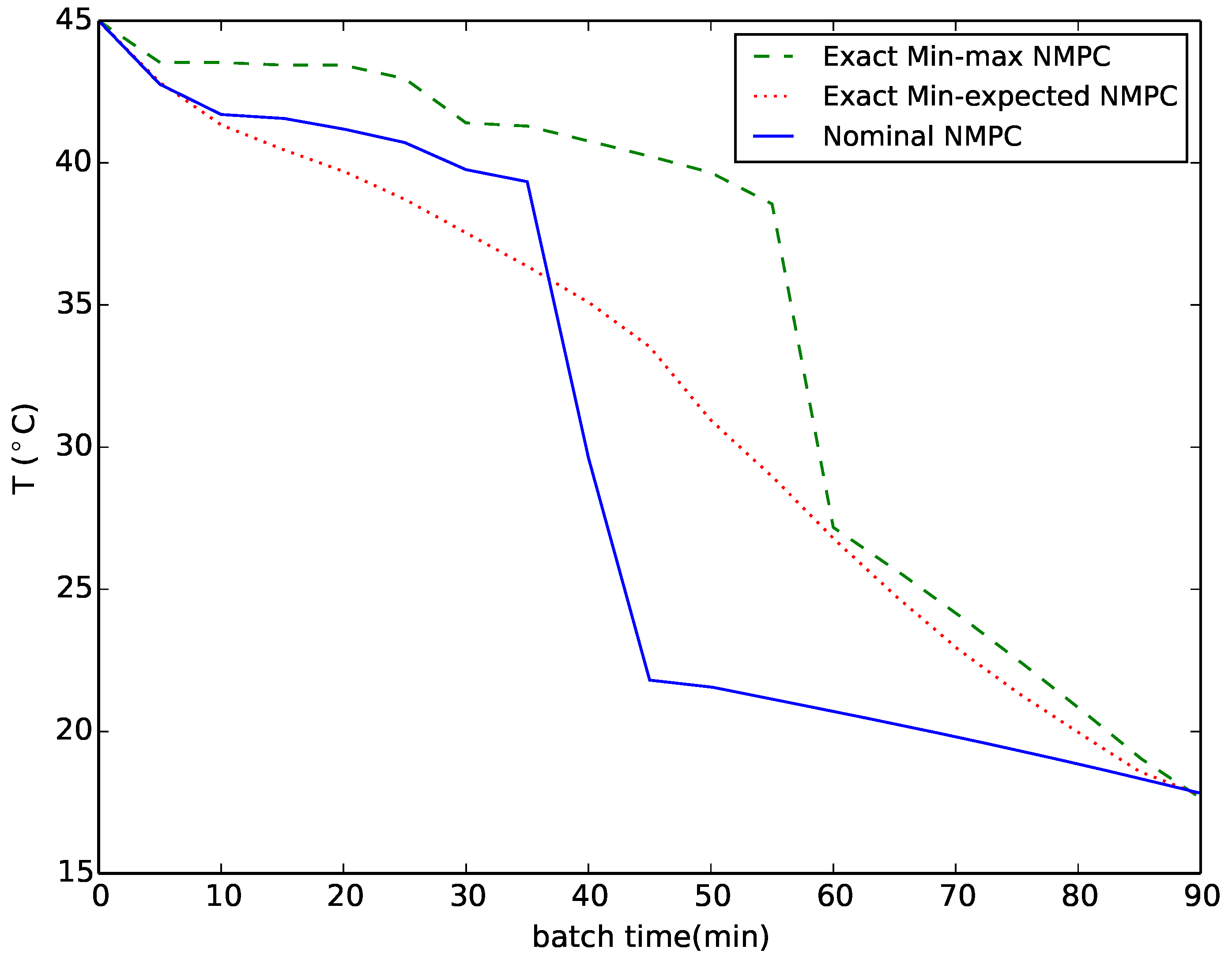
Figure 1. Optimal temperature profile for nominal NMPC (nonlinear model predictive control) and robust NMPC.
Processes 04 00020 g001
Table 1. The robust performance (value of c o s t ) of different control strategies evaluated using 100 test scenarios and exact information.
Control StrategiesNominalAverageStandard DeviationWorst-Case
Ideal 2 × 10 4 3066499
Open-loop 2 × 10 4 1672231339
Nominal NMPC0.293159955
Exact Min–max NMPC3278113677
Exact Min–expected NMPC12991691076
Table 2. The robust performance of the robust NMPC using different numbers of scenarios evaluated using 100 test scenarios.
TypeSNominalAverageStandard DeviationWorst-Case
Min–max2515991701062
50131021781129
751395156946
1002580120767
Min–expected252189138902
50111001721085
7512991691064
10012991691074
Table 3. The solution time of solving a robust optimization problem with 100 optimization scenarios.
# ProcessorsFull FactorizationSchur Complement Method
Time(s)Time(s)Speedup
Building Model144.364.2-
2-34.81.8
5-14.94.3
10-8.67.5
20-6.310.2
25-4.713.7
Solving NLP1406426.9-
2-216.32.0
5-90.84.7
10-51.08.4
20-35.811.9
25-30.014.2
Table 4. Robust performance of min–max NMPC with different numbers of optimization scenarios from Bayesian inference evaluated using 100 simulations.
TypeSNominalAverageStandard DeviationWorst-Case
Min–max121874120744
25136196584
501171114655
Min–expected121781141943
251284145949
501184145934