Article

Development of Chemical Process Design and Control for Sustainability

1
Department of Chemical and Biomedical Engineering, West Virginia University, Morgantown, WV 26506, USA
2
U.S. Environmental Protection Agency, Office of Research and Development, National Risk Management Research Laboratory, Cincinnati, OH 45268, USA
*
Author to whom correspondence should be addressed.
Processes 2016, 4(3), 23; https://doi.org/10.3390/pr4030023
Submission received: 11 April 2016 / Revised: 14 June 2016 / Accepted: 19 July 2016 / Published: 25 July 2016

Abstract

:
This contribution describes a novel process systems engineering framework that couples advanced control with sustainability evaluation for the optimization of process operations to minimize environmental impacts associated with products, materials and energy. The implemented control strategy combines a biologically-inspired method with optimal control concepts for finding more sustainable operating trajectories. The sustainability assessment of process operating points is carried out by using the U.S. EPA’s Gauging Reaction Effectiveness for the ENvironmental Sustainability of Chemistries with a multi-Objective Process Evaluator (GREENSCOPE) tool that provides scores for the selected indicators in the economic, material efficiency, environmental and energy areas. The indicator scores describe process performance on a sustainability measurement scale, effectively determining which operating point is more sustainable if there are more than several steady states for one specific product manufacturing. Through comparisons between a representative benchmark and the optimal steady states obtained through the implementation of the proposed controller, a systematic decision can be made in terms of whether the implementation of the controller is moving the process towards a more sustainable operation. The effectiveness of the proposed framework is illustrated through a case study of a continuous fermentation process for fuel production, whose material and energy time variation models are characterized by multiple steady states and oscillatory conditions.

Graphical Abstract

1. Introduction

Chemical industries have transformed the quality of human life rapidly by the chemical and physical transformation of ecological goods and services to higher economic value products, mostly without considering if those transformation routes or methods were more or less sustainable. In addition, renewability, scarcity and the impact of these material and energy resources were not accounted for during their use. Such contributions resulted in the development of practices based on critical materials (precious metal catalysts, fossil fuel based chemical precursors, heavy metals, persistent substances, etc.). The absence of sustainable economic practices has led to negative impacts on the environment and society from the release of persistent, toxic and hazardous substances to the air, water and land. In addition, unsustainable practices led to the fabrication of products without an adequate or responsible consideration of end-of-use and/or disposal. An early consideration of these aspects would make products feasible for their recycling, recovery or biodegradability.
Fortunately, this situation is changing since society, government and industry have realized that sustainable practices have the potential for obtaining economic benefits without harming the environment and human health. Many private and public initiatives started implementing a practice of sustainable development. Some of these components are related to energy saving or energy efficiency concepts, the use of renewable energy, etc. [1]. Other aspects are focused on material management approaches by the minimization of feedstock needs per unit of valuable product(s), reuse, recycling, renewable materials, etc. In particular, with the progress in understanding sustainability, the incorporation of sustainability into chemical process design, optimization and control has become a research highlight in process systems engineering recently [2].
Since sustainability is a holistic approach, belonging to an entire system beyond the manufacturing facility, sustainability assessment beyond the process can be carried out to decide which design alternative is more sustainable by performing life cycle assessment (LCA) considerations for identifying the greater life cycle impact contributing stages. However, the process manufacturing stage is where engineers have the opportunity to directly change process and product aspects that can improve indirectly the sustainability of the entire product life cycle [3]. In all of the life cycle product stages shown in Figure 1 occur fluctuation, variations and/or disturbances on the flow of energy, material and money that have to be measured, modified or kept at certain desired values in order to have a feasible business. Therefore, system control and optimization approaches play an important role in keeping the desired status quo of feasibility at macro (supply chain) and micro levels (product manufacturing). In addition, if that system status is sustainability performance and if this sustainability performance value needs to be improved or kept at a desired value, control and optimization for sustainability can be implemented.
Conventionally, process control and optimization approaches have been developed for achieving some economic objectives or cost minimization directly or indirectly. However, under sustainable development, not only economic aspects should be considered, social (safety, hazard free), environmental (pollution prevention and regulatory control), energy, material and economic performance aspects of the processes and products must be evaluated, optimized and controlled in order to meet sustainability goals. In addition, these process control approaches should act against unexpected instabilities when the process becomes unstable over time and/or due to changes in feed composition and flow rate, temperature and pressure. Process control and optimization should be able to perform transitions to different desired operating conditions and states to meet company and consumer demands, economics, process and product specifications (consumer or customer specifications), new environmental regulations, safety, managing low-dose chronic events, etc. Many researchers and engineers have contributed in an effort to develop systematic methodologies for sustainable process design, online/offline optimal search for sustainable operating conditions, as well as control strategies with the ability of improving the sustainability performance of chemical processes. In the last two decades, several emerging fields have been proposed in the area of sustainable design and optimization, such as process integration [4], process intensification [5], multi-objective optimization [6,7,8,9] and real-time operation along with sustainable corporate-scale management [10,11]. One common way to incorporate sustainability indicators (environmental and social aspects) into process design and optimization is to treat such indicators as constraints in the problem objective of maximizing profitability or minimizing the cost of the operations. For example, when minimum environmental risks/impacts related to non-routine and routine releases were considered, the optimal trade-off between cost and environmental impacts was obtained by employing the ε-constraint method, assuming the environmental impact targets were within ranges imposed by a selected amount defined by ε [12].
In addition, a hierarchical design procedure was proposed to synthesize economically-efficient separation processes, taking into consideration environmental factors as constraints [13]. Recently, a modular approach for sustainable chemical process design was developed through the integration of quantitative economics and environmental indicators with qualitative indicators in social aspects [14]. Compared to the aforementioned methods, multi-objective optimization schemes have a higher potential to obtain the optimal trade-off between conflicting economic and environmental objectives. For example, a global optimization method for sustainable design was developed, in which a large-scale algae processing network was simultaneously optimized in terms of minimizing the unit cost- and global warming potential-associated indicators [9]. Additionally, a multi-objective genetic algorithm was used to solve a single objective mixed integer nonlinear programming problem related to environmental impacts [6].
Noting the importance of taking process control into consideration at the design stage, some contributions have been made to the integration of sustainable process design and control by decomposition techniques. Specifically, a complex constrained optimization problem was formulated that included design, controllability, sustainability and economic aspects. This problem was decomposed into several sequential sub-problems to minimize its large computation cost [15,16]. Another study demonstrated the sustainability benefits of the integration of process design and plant-wide control for a continuous process of mono-isopropyl amine manufacturing [17]. In addition, several tools have been developed for control structure selection employing energy-related and sustainability concepts, as well as the thermodynamic property of exergy, such as the relative exergy array (REA), exergy eco-efficiency factor (EEF) and relative exergy destroyed array (REDA) [18]. However, research in sustainable process control for chemical processes is not yet as established as sustainable design and optimization. There are only a few reported studies on process operations employing sustainability-oriented control strategies. In particular, a method integrating deterministic dynamic optimization with optimal control was proposed to address the sustainability of a batch reactor [10,11]. Another application of deterministic optimal control strategies was reported to improve energy efficiency in manufacturing processes [19]. In these two studies, only utilities-related environmental impacts were considered. This limitation can be attributed to the lack of effective strategies that can integrate process sustainability aspects into the advanced controller framework, considering the conflicting nature of sustainable indicators (e.g., economics vs. environment) [20].
As a step forward to address this gap in the research and development fields, here, we propose a novel framework for process systems that integrates an advanced process control strategy with sustainability assessment tools. The developed framework is employed to identify and assess the optimal process operation in terms of sustainability performance. Specifically, a set of steady-state alternatives for the chemical process is generated through the implementation of the advanced biomimetic control strategy, and the obtained process operating points are evaluated employing the indicators from the GREENSCOPE assessment tool [21] in efficiency, environmental, energy and economic aspects. Such a comprehensive assessment of sustainability performance provides information on quantifying the benefits that the implementation of the biomimetic controller brings towards achieving a more sustainable process operation. The developed framework is applied to a fermentation process for bioethanol production. The problem’s objective function is formulated to minimize the differences between product concentration and reactor temperature (as key state variables) and their set points. The sustainability performance of the process after the controller implementation is then evaluated through selected GREENSCOPE indicators. The outline of the rest of this paper is as follows: the sustainability assessment tools and indicators are presented in the next section, followed by the advanced controller development and algorithm. These tools provide a general framework for optimizing and controlling chemical processes in terms of sustainability. Then, the proposed approach is implemented for the case study of a fermentation process involving Zymomonas mobilis. The paper is closed with conclusions.

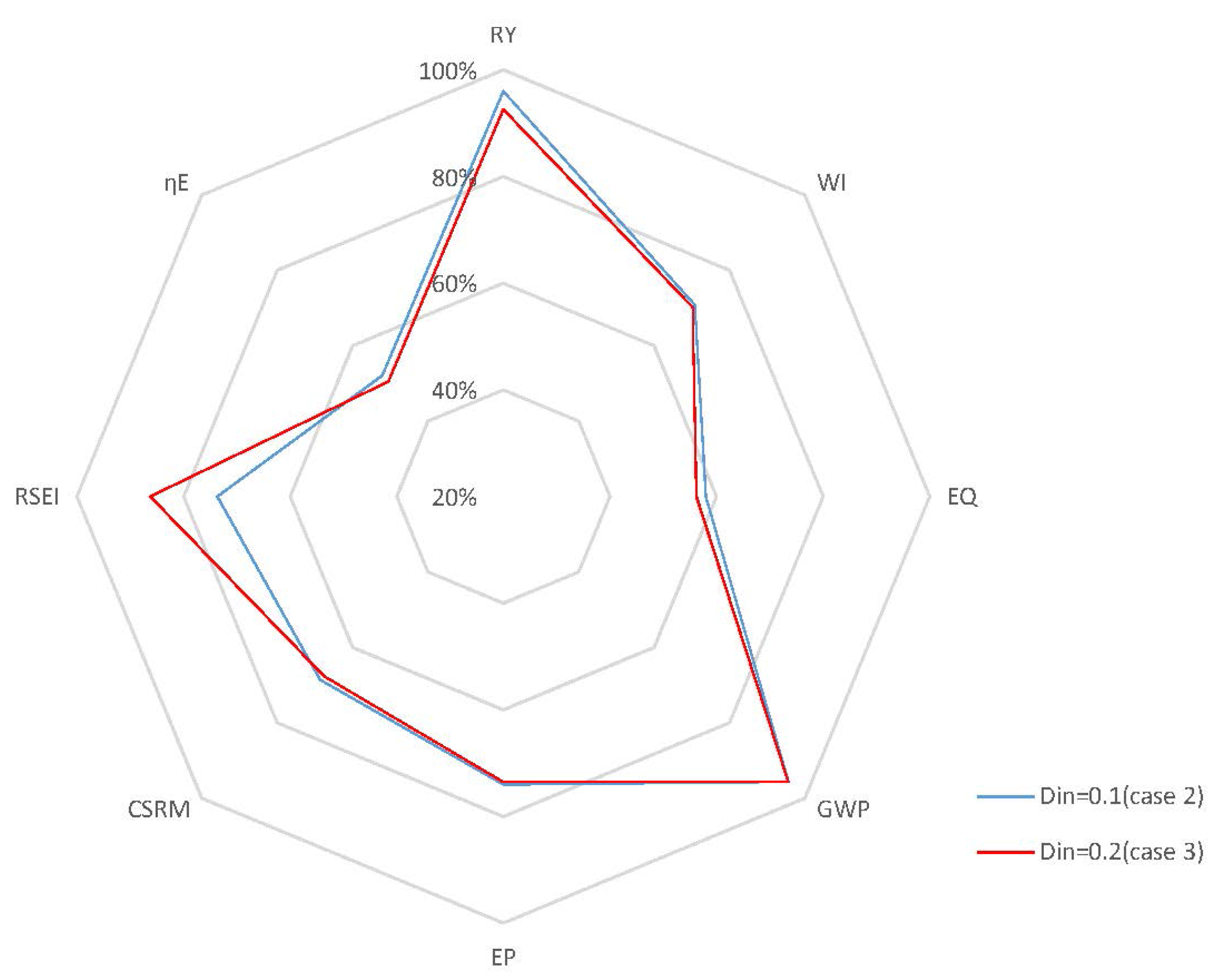
2. Process Sustainability Assessment and Design

As stated by the green chemistry and engineering principles [22,23], chemical processes and products that reduce or eliminate the use and generation of hazardous substances should be developed by preventing waste, performing real-time analysis and control for pollution and accident prevention, maximizing mass, energy, space and time efficiency, etc. [3]. In addition, when a more sustainable performance is achieved, this must be ensured under any type of beyond the gate (front-edge changes) and/or process stage perturbations.
As mentioned above, society, government and industry have created initiatives regarding the implementation in practice of sustainable development. However, it is often unclear what the effects (positive or negative) of these new practices would be in the environment. In order to offer a more comprehensive and quantitative description of environmental, social and economic effects, the U.S. EPA has proposed a tool called GREENSCOPE [21] (Gauging Reaction Effectiveness for the ENvironmental Sustainability of Chemistries with a multi-Objective Process Evaluator) to support decision makers when developing, designing and evaluating sustainable processes and products. The GREENSCOPE tool allows for quantifying process sustainability and life cycle inventory (LCI) generation with about 140 indicators in four main areas: material efficiency (26), energy (14), economics (33) and environment (66). These indicators are capable of transmitting and translating process performance, feedstocks, utilities, equipment and output information into a sustainability measurement scale. GREENSCOPE is designed to directly provide process-specific data into life cycle assessment databases for conducting LCAs. As mentioned before, LCI is an important step in the development of LCAs, which determine environmental effects throughout a product’s life cycle stages.
GREENSCOPE can be applied to equipment or process units, as well as to the entire process or bench scale, allowing for a direct comparison between several processes manufacturing the same product, but employing different raw materials, reaction processes and separation technologies and producing different byproducts. In addition, the designer or the researcher can implement this methodology to evaluate the sustainability performance after making process modifications.
A biodiesel production case study demonstration using GREENSCOPE was performed [21,24] to provide decision makers guidance on using this assessment and design tool, from sustainability indicators [25] and their data entries [26] to sustainability evaluation outcomes and the related life cycle inventory generation. The tool can then show which indicators have improved and where additional opportunities for improvement exist. The indicator scores describe product and process performance on a sustainability measurement scale, determining whether chemical products and processes are more or less sustainable. The scale for measuring sustainability is developed according to the identification and use of the best possible target (100% of sustainability) and a worst-case scenario (0% of sustainability) as reference states [25], in other words, as the upper and lower bounds of a sustainability measurement scale. This sustainability scale allows the transformation of the process performance indicator scores to a dimensionless form using the worst and best scenarios [27,28] as follows:
P e r c e n t   S c o r e =   | A c t u a l W o r s t | | B e s t W o r s t | × 100 %
This equation helps to visualize and compare the sustainability assessment results of each indicator during the process or product analysis. In other words, this sustainability assessment describes how well the system under consideration makes use of mass and energy inputs to manufacture a valuable product, meeting social and environmental needs, while maximizing its economic benefits.

3. Novel Advanced Control Approach

Many biological systems have been a source of inspiration for advanced control methods because of the success of these systems in solving difficult problems encountered in nature. In this section, an advanced biomimetic control approach to address the challenges involved in chemical processes is briefly described. This approach is the combination of a biologically-inspired multi-agent-based algorithm with optimal control concepts for the calculation of optimal trajectories of individual agents. The multi-agent-based algorithm is essentially inspired by the ants’ rule of pursuit idea [29], which is shown schematically in Figure 2. As per this ants’ rule, the first ant is supposed to find food by walking around at random. This pioneer ant would then trace a wiggly path back to the nest and start “group recruitment”. The subsequent ants (or agents) would follow one after the other, straightening the trail a little starting from the original path until the agents’ paths converge to a line connecting the nest and the food source, despite the individual ant’s lack of sense of geometry. Thus, by cooperating in large numbers, ants (or agents) accomplish tasks that would be difficult to achieve individually. This is an excellent example of how biological systems can efficiently solve problems encountered in nature by cooperative behavior.
This idea serves as inspiration for the development of a novel optimal control approach for chemical systems to reach the optimal operating point in terms of sustainability. To translate this idea into an optimal control algorithm, we first define a chemical system with a dynamic model represented by ordinary differential equations and differential-algebraic equations. This dynamic model corresponds to a relationship between the state and control/input variables. The agent’s “home” is the initial conditions for each variable while the “food” stands for the desired operating point of the system. The solution of the optimal control problem for each agent gives the trajectories of these variables to connect home to food through an optimized control action. Next, we assume there is an available initially feasible trajectory pair for the state and control variables, which is obtained through prior knowledge of the system. This trajectory corresponds to Agent 0 (a0) or the leader’s trajectory for the initialization of the algorithm. In addition, two important parameters that define the leader-follower local interactions need to be specified, the pursuit time, Δ, and the sampling time, δ.
The initial conditions for each state variable of the follower are the follower’s trajectory points based on the discretization by the sampling time, δ. The final destination for the follower agent is obtained from the leader’s trajectory discretization based on the sampling time, δ, as well as the pursuit time, Δ, explained in Figure 3. The initial conditions and the final destinations are provided to the optimal control solver, in this case dynopt, for the computation of the optimal trajectories. Specifically, dynopt is a set of MATLAB functions that use the orthogonal collocation on finite elements method for the determination of optimal control trajectories. The inputs of this toolbox are the dynamic process model, the objective function to be minimized and the set of equality and inequality constraints. The outputs from this toolbox are the optimal control laws and state trajectories. For the first step calculation, the optimal control trajectories of each follower are computed numerically using dynopt by looking at the leader’s position at Δ time units as the current target. The obtained control law is then applied for δ time units, before repeating the procedure outlined in Figure 3. The developed algorithm employs dynopt to solve the intermediate problems associated with the local interaction of the agents to generate the state and the optimal control trajectories.

4. New Approach for Process Modeling and Advanced Control for Sustainability

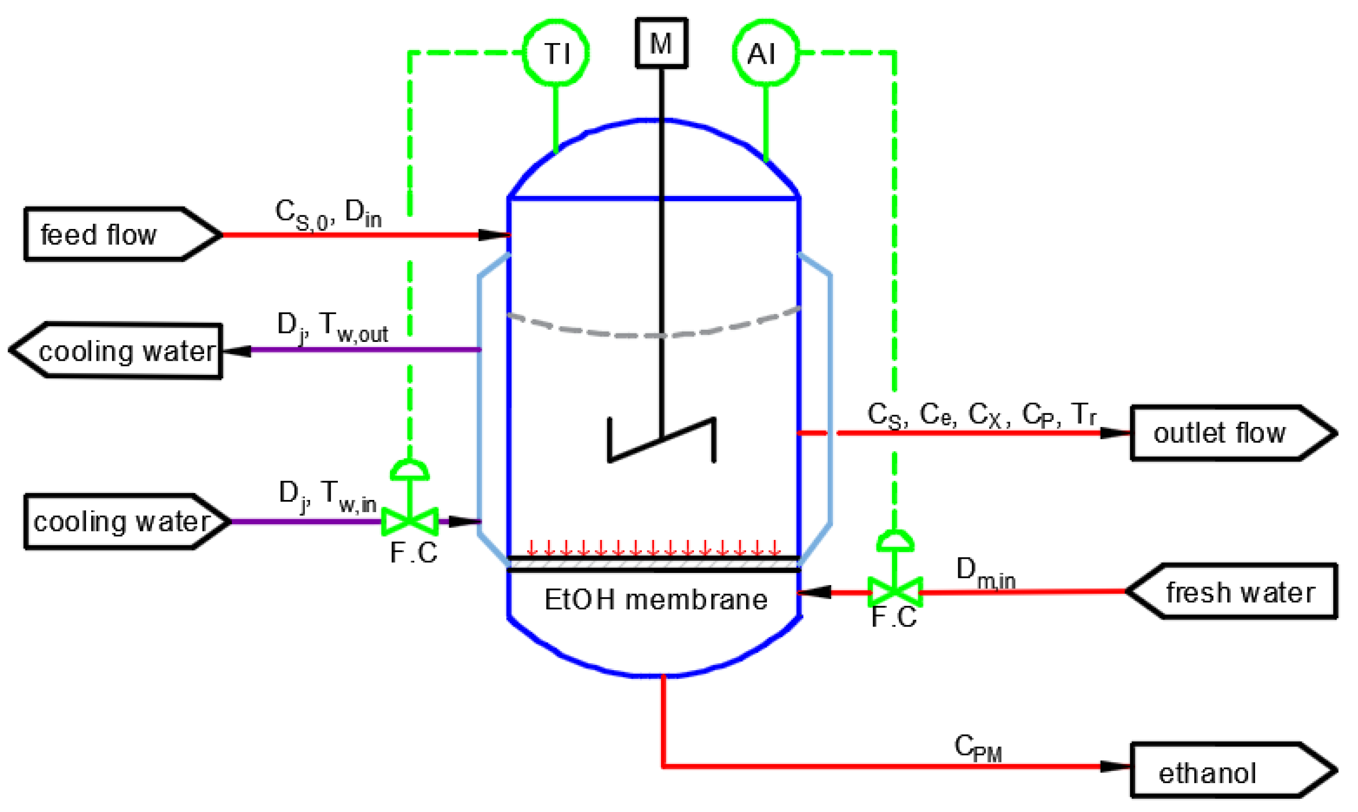
4.1. Bioethanol Manufacturing Process Model

Ethanol derived from renewable sources, such as corn, sugar cane and beets is a potential sustainable fuel to control and decrease air pollution from internal combustion engines and reduce the dependence on fossil fuels. Herein, we consider a process model for a homogeneous, perfectly-mixed continuous culture fermentor for ethanol production equipped with an ethanol-selective removal membrane and a cooling jacket for temperature control. A schematic diagram of the fermentation reactor is shown in Figure 4. The reactor is modeled as a continuous stirred tank (CSTR) with constant substrate feed flow. The outlet flow from the reactor contains the product, the unreacted substrate, as well as biomass. Biomass plays the role of catalyst for substrate conversion and is the product of fermentation, while the substrate is a solution of glucose for feeding the micro-organism (in this case, Zymomonas mobilis). Moreover, ethanol is the desired product of the process and an inhibitor for the enzymatic reactions. To prevent end-product inhibition and improve the productivity and efficiency of the fermentation process, an in situ ethanol-removal membrane is used so that the ethanol is removed as it is being produced.
The ethanol fermentation process involves living microorganisms and has two main reactions: (1) microbial growth reaction, in which a certain amount of substrate is consumed for the growth of biomass under favorable environmental conditions (temperature, pH, etc.); and (2) metabolite reaction, in which substrate (referred to as reactant) is converted into product through the catalytic action of enzymes. For process design and control purposes, several models for fermentation processes are available in the literature based on the kinetic expressions of different complexity [30,31,32,33]. For example, cellular components, enzymes and proteins can be used to express the process kinetics. However, typical models consider only the kinetic expressions of fermentation for constant temperature conditions. The proposed mathematical model here takes into consideration the temperature effect on kinetics parameters, mass and heat transfer, in addition to the kinetic equations modified from the indirect inhibition structural model developed in the literature [34,35].
In this structural model, it is assumed that the inhibition effect of ethanol is on the formation of a key component (that includes RNA and proteins in biomass), instead of directly on fermentation. To accurately describe the formation rate of the key component at low ethanol concentrations and under substrate-limited conditions, the formation rate expression for the key component [34,35] is a function of substrate concentration, given by:
r e = f ( C P ) f ( C S ) C e
A Monod-type equation is taken for f ( C S ) :
f ( C S ) = C S K S + C S
The function f ( C p ) is empirically described by a second-order polynomial of the following form:
f ( C P ) = k 1 k 2 C P + k 3 C P 2
The expressions for biomass growth rate and substrate consumption rate can be taken from the classic maintenance model [36], where the biomass growth rate is defined as:
r X = μ C X
in which μ , as the specific growth rate, can be expressed as follows:
μ = μ m a x · C S ( K S + C S )
In addition, the substrate consumption rate can be written as:
r S = ( 1 Y s x ) r X + m s C X
in which the first term accounts for the growth of biomass, while the second term for the maintenance of biomass.
The expression for the maximum specific growth rate, μ m a x , involves the ratio of the key component to biomass and the temperature effect:
μ m a x = P · C e C X · f ( T )
in which P is a correction factor and f ( T ) can be obtained by fitting a set of experimental data from the literature [37] to the following equation:
f ( T ) = A 1 · e E a 1 R T A 2 · e E a 2 R T
The dynamic mass balances for the key component, biomass and substrate are expressed by:
d C e d t = ( k 1 k 2 C P + k 3 C p 2 ) C S C e ( K S + C S ) + D i n C e , 0 D o u t C e
d C X d t = P · f ( T ) · C S C e K S + C S + D i n C X , 0 D o u t C X
d C S d t = ( P Y s x ) · f ( T ) · C S C e ( K S + C S ) m s C X + D i n C S , 0 D o u t C S
As the product flows out of the system through the fermentor and the membrane, mass balances are derived for the product in both compartments and are given by:
d C P d t = ( P Y p x ) · f ( T ) · C S C e ( K S + C S ) + m p C X + D i n C P , 0 D o u t C P ( α V F ) ( C P C P M )
d C P M d t = ( α V M ) ( C P C P M ) + D m , i n C P M , 0 D m , o u t C P M
in which:
α = A M · P M
Using the overall mass balances for the fermentor and membrane, the outlet dilution rates for both compartments are respectively defined as:
D o u t = D i n α · ( C P C P M ) V F · ρ r
D m , o u t = D m , i n + α · ( C P C P M ) V M · ρ r
Moreover, the energy balances for the reactor and the cooling jacket are the following:
d T r d t = D i n ( T i n T r ) + r S · Δ H ρ r · c p , r K T A T · ( T r T j ) V F ρ r · c p , r
d T j d t = D j ( T w , i n T j ) + K T A T · ( T r T j ) V j ρ w · c p , w
Thus, the derived mathematical model for the fermentation process is represented by a set of seven ordinary differential equations for key component, biomass, substrate, product and temperature and two algebraic equations of outlet dilution rates. Table 1 provides the parameter values of the model and the initial operating conditions used in this Zymomonas mobilis fermentation problem (see all variables’ definitions and units in the Nomenclature section).

4.2. Case Study: Fermentation for Bioethanol Production System

For the Zymomonas mobilis fermentation process addressed here, sustained oscillations of biomass, substrate and product profiles have been widely reported [38,39]. An effective controller is therefore required to eliminate oscillations and to take the process to an optimal operating steady state. However, the design and implementation of a high-performance control algorithm for this fermentation process in terms of productivity and sustainability is a challenging task, mainly due to its highly nonlinear dynamics. To address these challenges, this section introduces a new process control for the sustainability framework that combines the biomimetic control strategy detailed above with the GREENSCOPE sustainability assessment tool. In the performed case studies, the purpose of the implemented biomimetic controller is to keep key state variables at their set points through the optimization of the control actions. Thus, in this case, the objective function is formulated to minimize the differences between product concentration and temperature (as key state variables) and their set points. The sustainability performance of the process after the controller implementation can then be evaluated through selected GREENSCOPE indicators shown in the Appendix (see Table A1 for indicator details). Specifically, the obtained GREENSCOPE indicator scores provide information on whether the implementation of the biomimetic controller for the fermentation process enables a more sustainable process operation when compared to a benchmark.

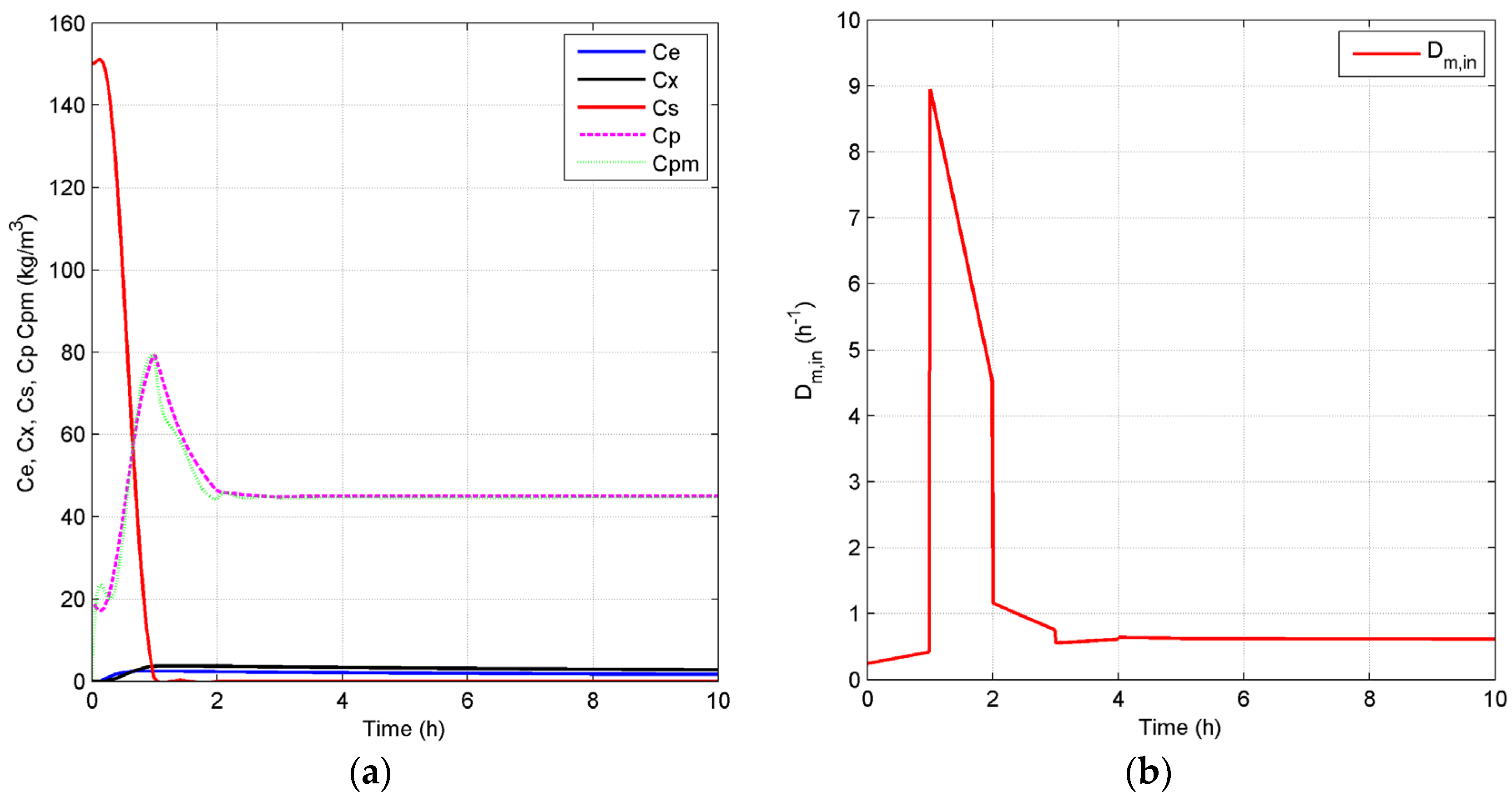
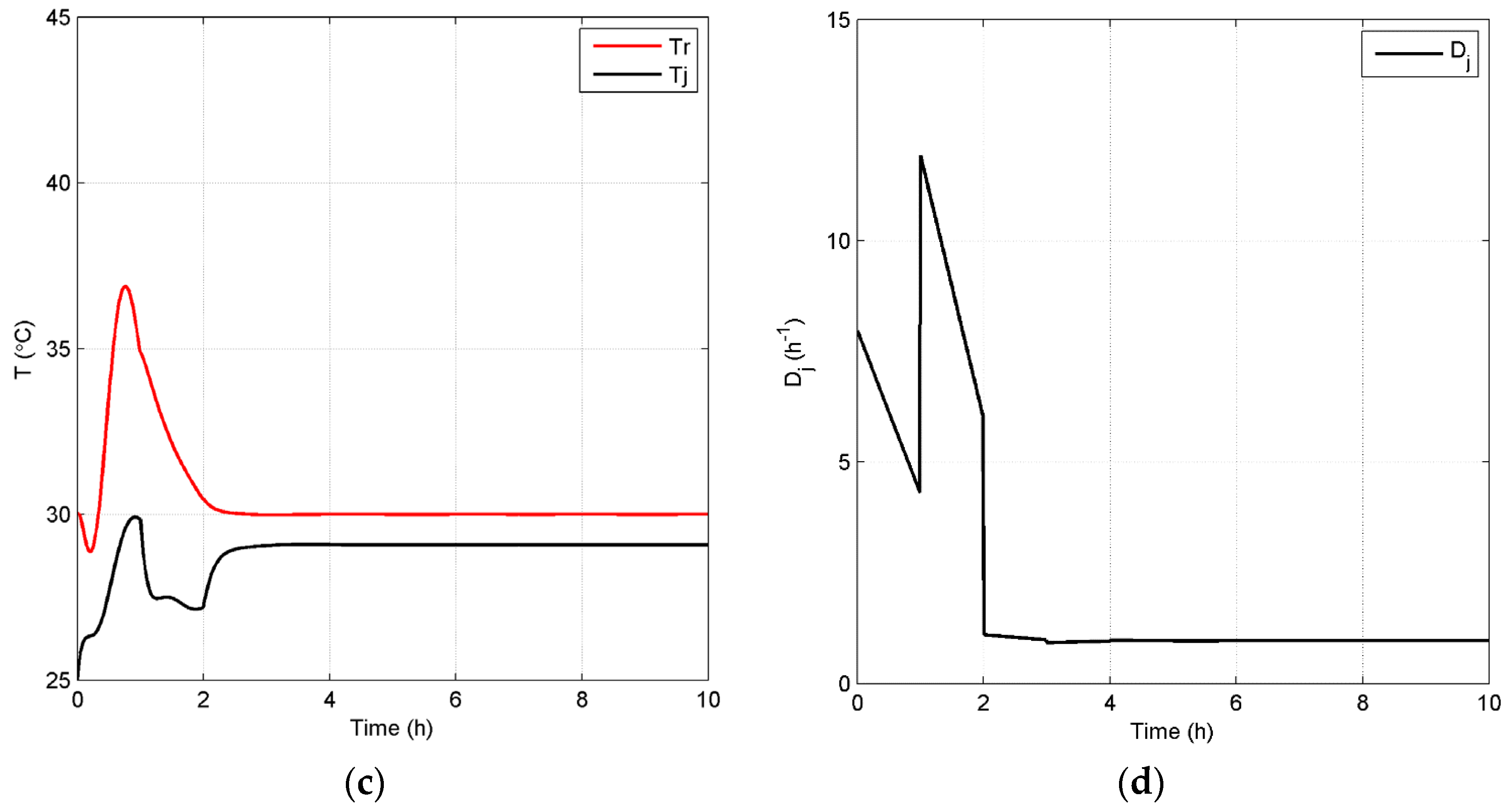
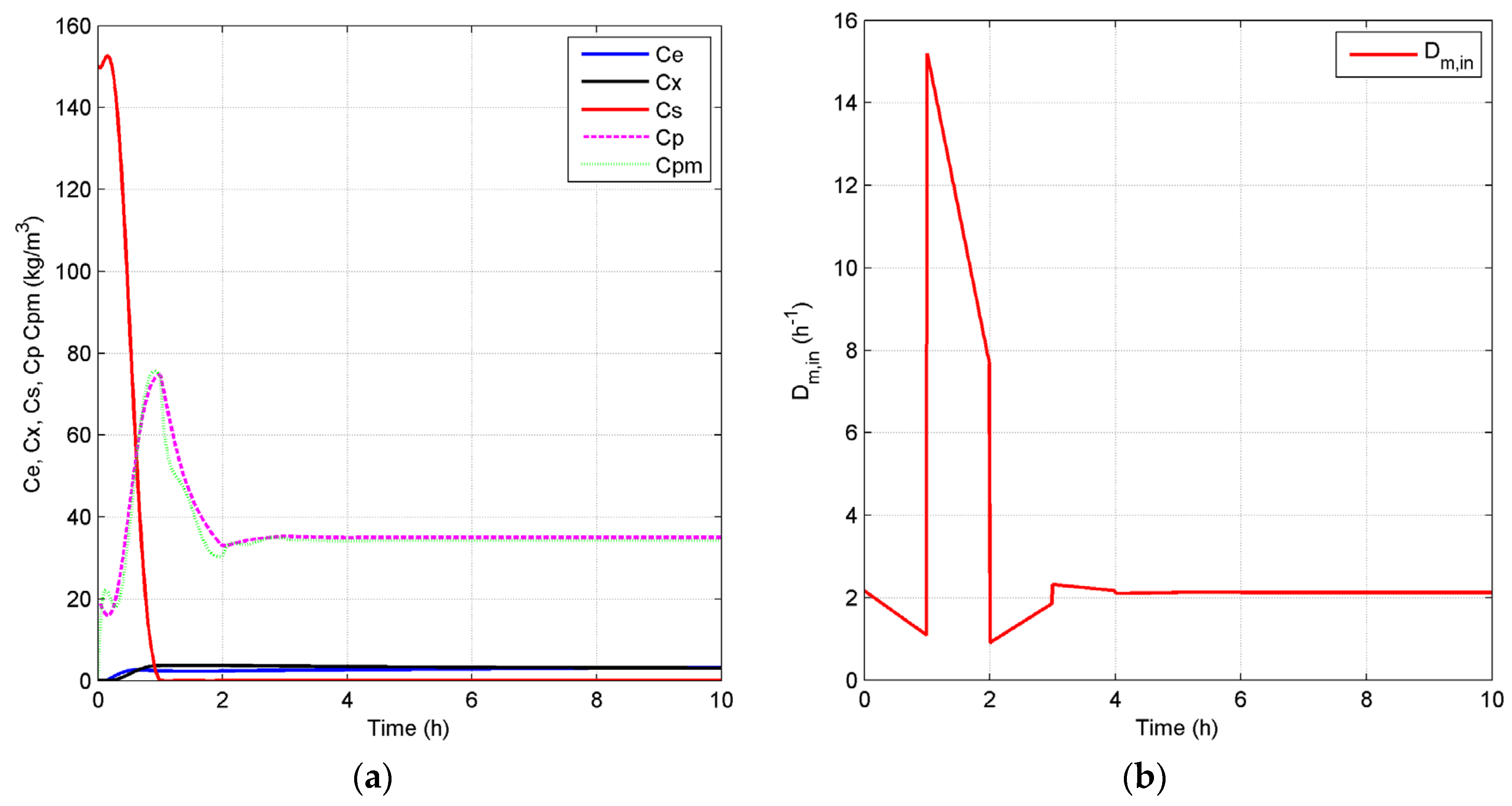
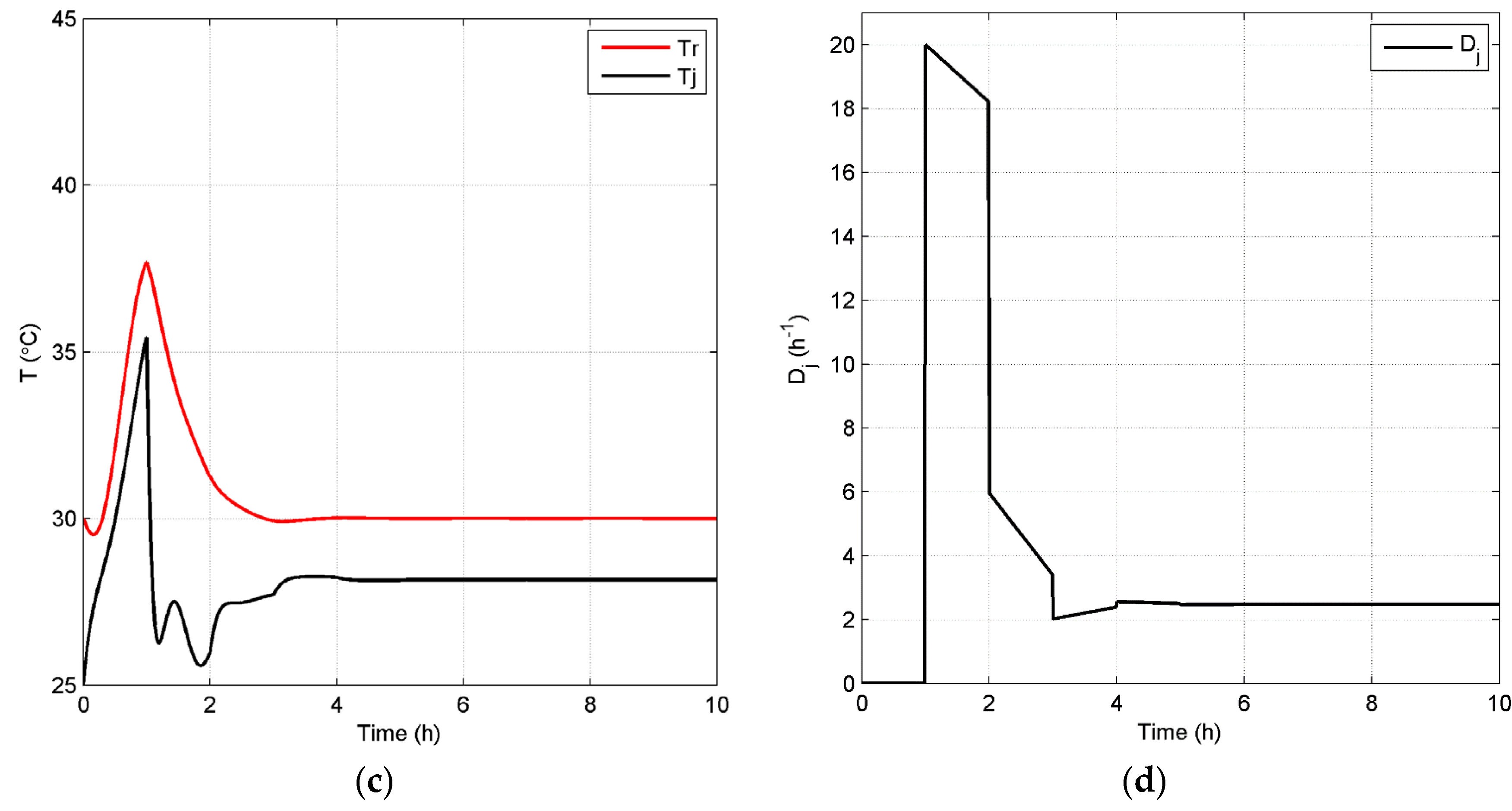
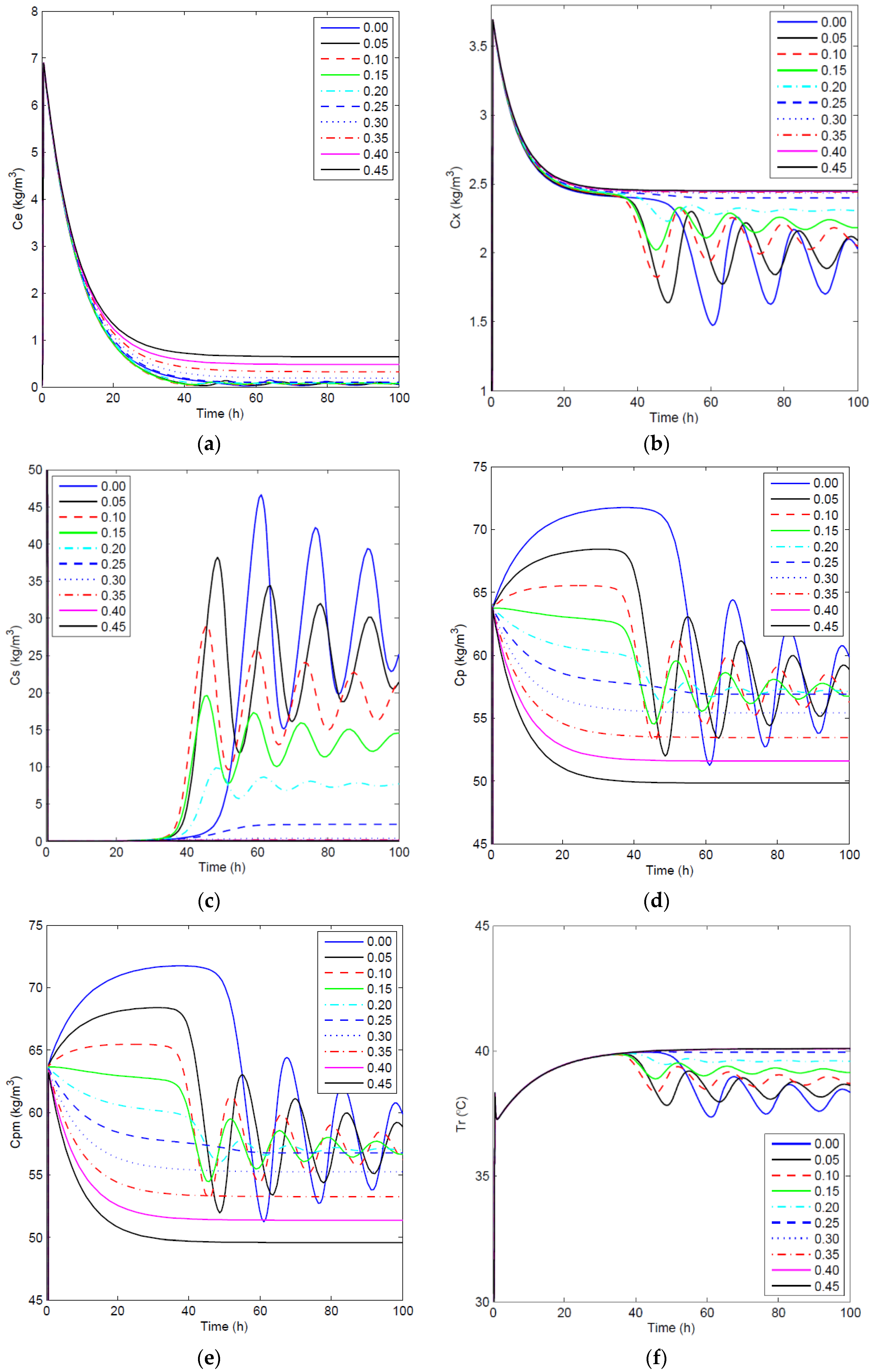
4.2.1. Open-Loop Dynamics of Fermentation Process

Before the implementation of the process control for the sustainability framework, it is worth analyzing the dynamics of the fermentation process. In agreement with the literature, the results of open-loop simulations in Figure 5 show that oscillations are more prone to occur at high ethanol concentrations due to the end-product inhibition effect. Ethanol has great impact on the cell membrane composition and inhibits enzymatic reactions. Temperature, as another important operating variable, not only affects the activity of biomass, but indicates the energy consumed by the process affecting its economic performance. Thus, an attractive control strategy consists of regulating the concentration of product and the reactor temperature at optimal operating points in terms of process sustainability and productivity. The present study is an extension of previous work regarding the fermentation process that had a strategy of controlling product concentration through manipulating D i n [27]. In this paper, the membrane dilution rate, D m , i n , as well as the cooling water flow rate, D j , are chosen as the manipulated variables for the regulation of ethanol concentration, C P , and fermentor temperature, T r , respectively. It is shown below that using D m , i n as the manipulated variable is an efficient way to stabilize the system and improve the productivity of the reactor.
To analyze the effect of D m , i n on the fermentation process, open-loop simulations were completed in which D m , i n varied from 0 to 0.45 h−1, and D j was set to zero. For these simulations, the system was integrated using the ode 15 s solver in MATLAB (Version 8.3, MathWorks, Inc., Natick, MA, USA) for the given differential and algebraic equations that were solved simultaneously. Figure 5 shows the concentration profiles of the key component, biomass, substrate, product in the fermentor and membrane sides, as well as temperature profiles in the fermentor for the open-loop simulations with different membrane dilution rates. As expected, a higher D m , i n can efficiently reduce or even eliminate the oscillatory behavior of the concentrations and can enhance the substrate conversion rate. This can be explained by the reduction of the end-product inhibition when more ethanol is removed through the ethanol-selective membrane at the cost of using more fresh water. It is important to note that this fermentation process has multiple equilibrium states as a consequence of autocatalytic reactions [40]. To obtain an optimal steady-state operating condition in terms of sustainability and examine the effectiveness of the proposed biomimetic controller, an open-loop case is chosen as the benchmark, and then, higher and lower set points are used for closed-loop simulations. Through the comparison of the GREENSCOPE indicators for the benchmark and closed-loop simulations, a systematic decision can be made in terms of moving the process operation in the right direction towards a more sustainable steady state.

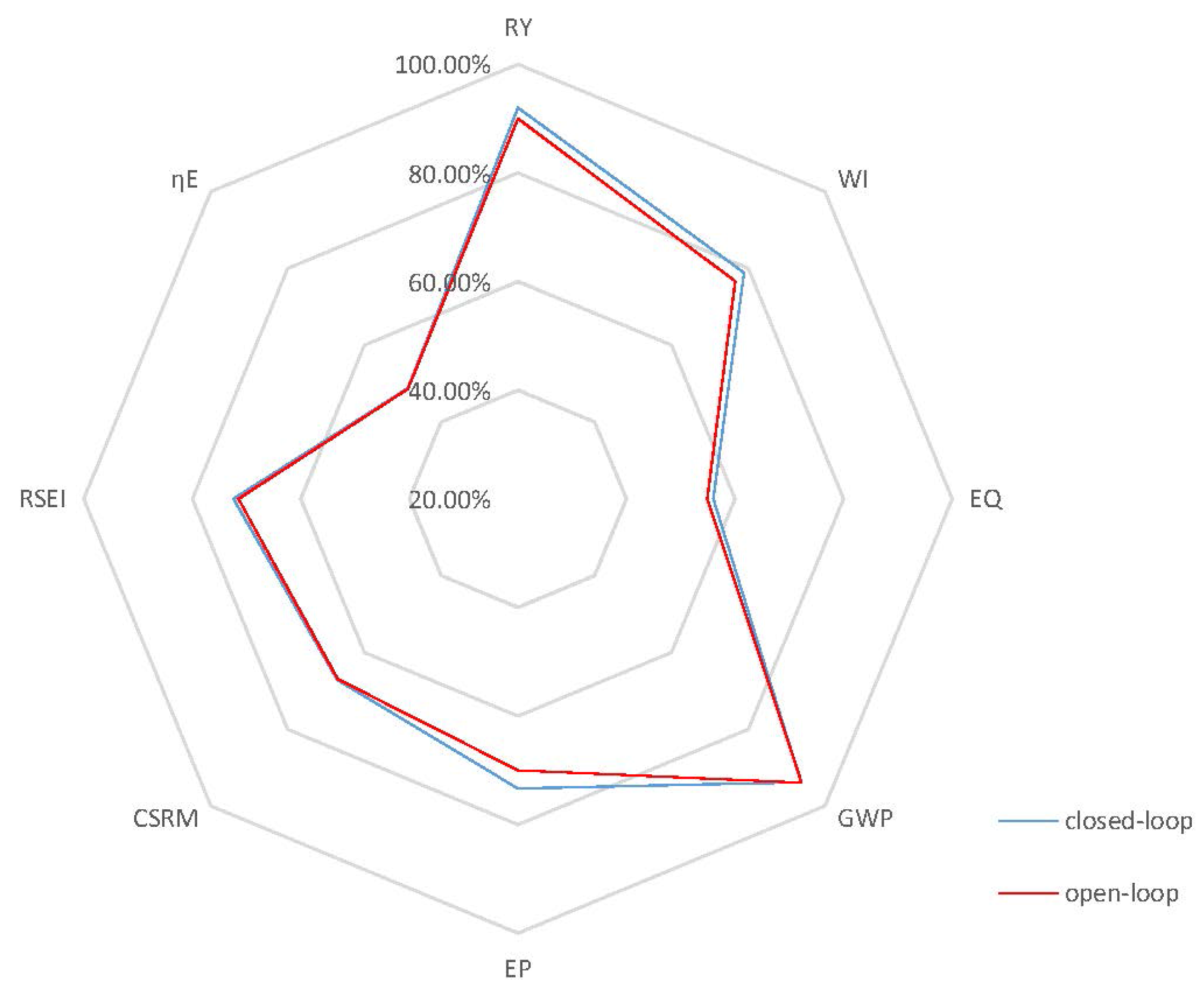
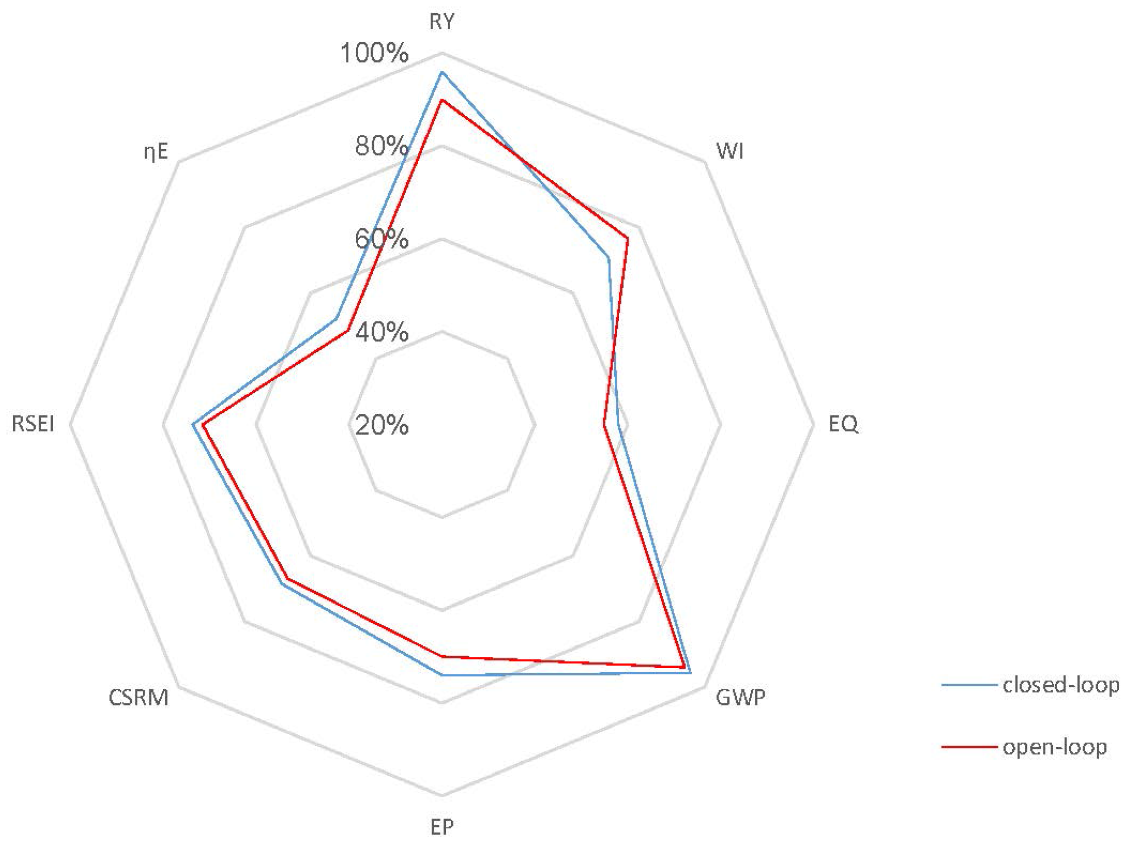
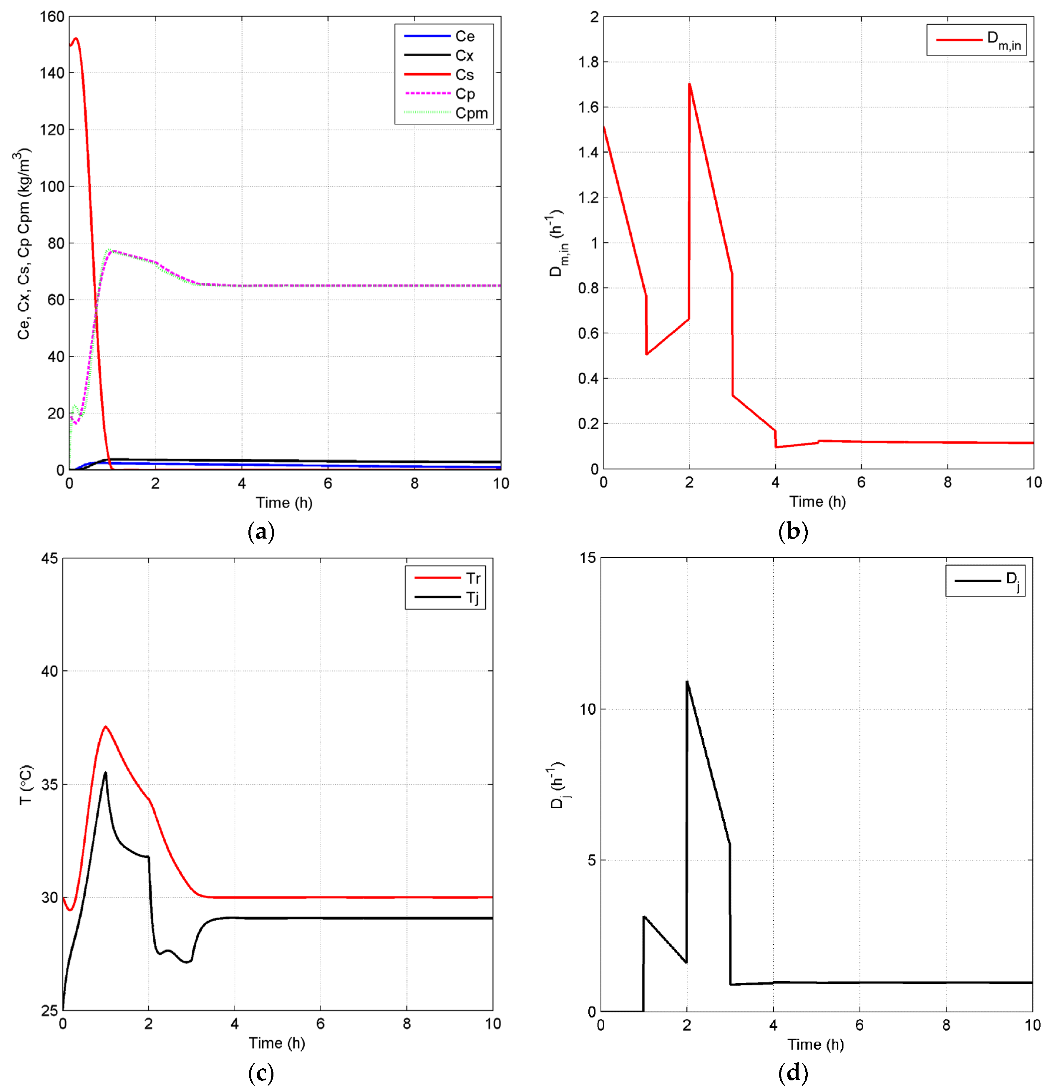
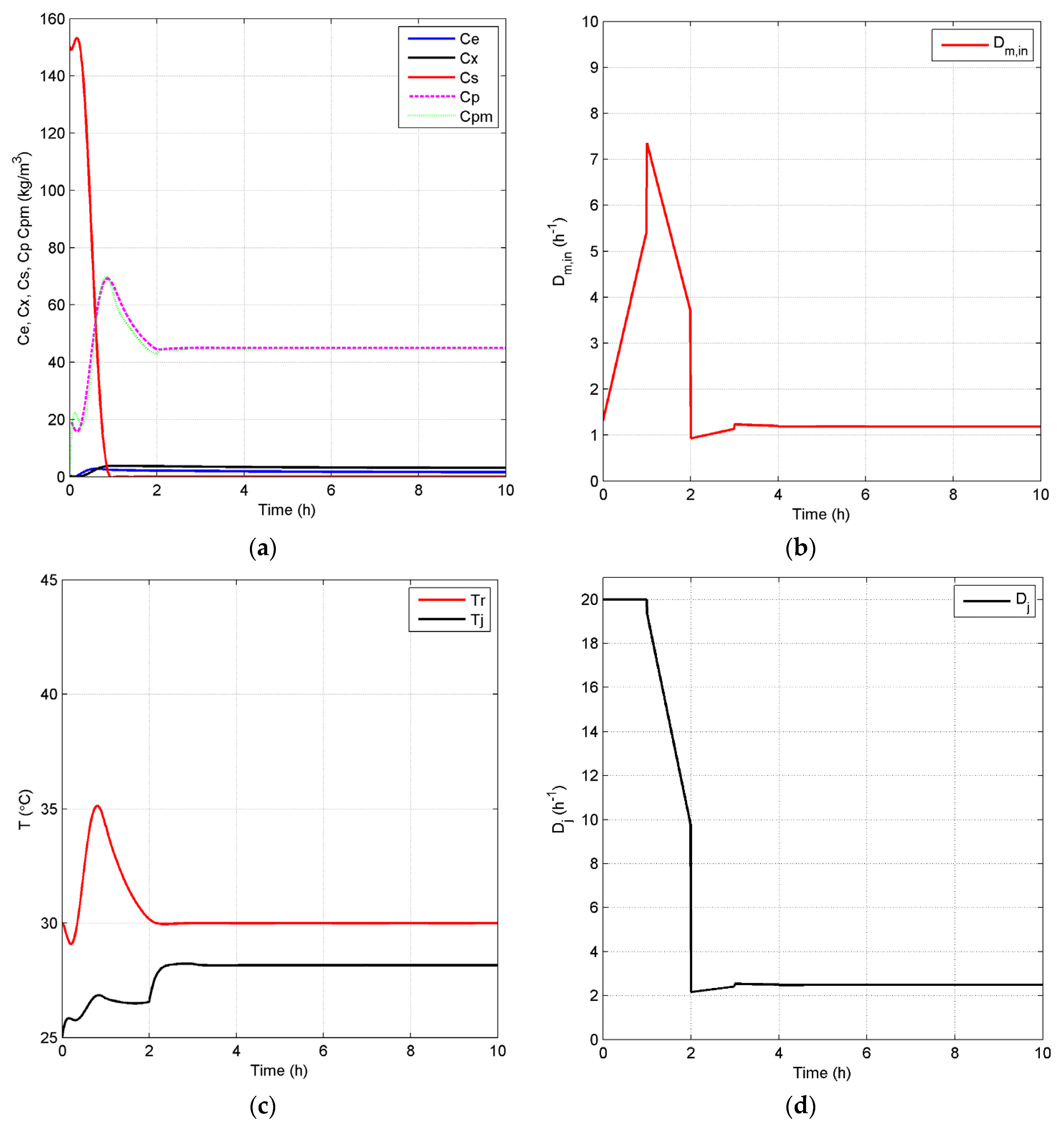
4.2.2. Closed-Loop Results and Discussion

Four case studies are presented here to evaluate the implementation of this novel process control for sustainability framework. The first two cases are designed to demonstrate the effectiveness of the implementation of the proposed controller by its ability to take the system to higher and lower set points when compared to the benchmark within the shortest response time possible. These cases use an initial D i n value of 0.1 h−1. The new achieved steady states are evaluated and compared in terms of sustainability using selected GREENSCOPE indicators. Based on the results of the first two cases, Cases 3 and 4 are then performed to locate the optimal steady-state operation for a higher D i n of 0.2 h−1, which corresponds to a higher volumetric productivity for the fermentor. For all simulations, the parameter values in Table 1 are kept constant.
Case 1: In case 1, the open-loop simulation with D m , i n of 0.20 h−1 is chosen as the benchmark since it represents the highest achievable product concentration with reduced oscillations, as it approaches the steady state. In particular, for this case, the dynamic behavior in Figure 5 shows oscillations of mid-range amplitudes within 80 h before the system finally achieves its steady state at around 100 h. It is important to note that there is still some substrate left in the reactor at steady state as depicted in the substrate profile of Figure 5. This can be explained by the fact that the environmental conditions in this case, such as temperature and ethanol concentration, are not favorable for a high substrate conversion rate. Thus, there should be some room for improvement of process performance by the implementation of an effective control strategy in terms of efficiency and productivity, if the system is optimized to convert all substrate into product. To attain this goal of increasing the process efficiency, a higher set point for the controlled variable, C P , of 65 kg/m3, when compared to the steady-state product concentration of the benchmark case, 57.16 kg/m3, is used. In addition, an optimal temperature value, 30 °C, for T r is employed in the closed-loop simulation. Both open-loop and closed-loop simulations start at the same initial points, and the inlet dilution rate, D i n , is kept at 0.1 h−1. Figure 6 depicts the closed-loop simulation results for the concentrations of key component, biomass, substrate, product and temperature, as well as the input profiles. Note that, with the implementation of the proposed biomimetic control strategy, the original oscillations are eliminated, and merely a trace of substrate unreacted, 0.043 kg/m3, is left in the reactor. However, in terms of sustainable performance, the radar plot of Figure 7 shows that the controller implementation only slightly improves three GREENSCOPE indicators in three categories (efficiency, economic, and environmental), reaction yield (RY), water intensity (WI) and economic potential (EP), towards a more sustainable process operation. In addition to Table A1 in the Appendix, more details regarding indicator definition (qualitative and quantitative), data inputs and best and worst case reference values can be found elsewhere [25,26,27]. Another key aspect is the steady-state biomass concentration is 2.50 kg/m3 in the closed-loop simulation, which is higher than the open-loop simulation, 2.31 kg/m3. This higher value means that more substrate is consumed for biomass growth, rather than for producing ethanol in the new scenario. This fact explains why some of the other indicators, such as resource energy efficient (ηE) and specific resources material costs (CSRM), do not show improvement even though the substrate conversion rate increased by 5.1%.
Case 2: As discussed above, ethanol concentration and temperature have a great effect on the living biomass, and thus, controlling the reaction environment at optimal conditions can enable higher fermentation process efficiency. Based on the fact that a lower product concentration may reduce the effect of product inhibition, we define a lower value of C P = 45 kg/m3 as the set point for the closed-loop scenario and keep the set point of T r at 30 °C in Case 2. Figure 8 shows the concentration and temperature profiles, as well as the input profiles for the closed-loop simulation. Compared to the results in Figure 6a, Figure 8a shows that the system reaches the steady state in this case in a shorter time and with a lower substrate concentration of 0.03 kg/m3. In addition, the steady state D m , i n increases to 0.61 h−1, which means that more ethanol is removed by the membrane to keep a lower ethanol concentration in the reactor. All GREENSCOPE indicators except water intensity (WI) in Figure 9, such as reaction yield (RY), environmental quotient (EQ), environmental potential (EP), specific raw material costs (CSRM), specific energy intensity (RSEI) and resource energy efficiency (ηE), demonstrate the higher degree of sustainability for the closed-loop scenario. This improvement of sustainability performance can be attributed to the elimination of oscillations and removal of the inhibition effect by the product after the implementation of the biomimetic control strategy.
Case 3: It is documented that fermentation processes are characterized by the conflict between the yield of the desired product and the productivity of the reactor, which are both important performance indicators from a stakeholders’ commercial point of view [40]. Operating points that correspond to a good trade-off between yield and productivity may be achieved, if the fermentation process is optimized by manipulating D i n . In our previous work, it was shown that a high D i n generates high productivity, but with a low yield due to the end-product inhibition [27]. One advantage of using D m , i n as a manipulated variable, however, is reducing the coupling between yield and productivity. Based on this information, for this case study, a closed-loop simulation with D i n of 0.2 h−1 is studied, where the set points are kept at the same values as in Case 2. Figure 10 presents the concentrations of key component, biomass, substrate, product and temperature, as well as the input profiles for the closed-loop simulation in this case. When compared to the results of Case 2, which are depicted in Figure 8, the closed-loop scenario in this case shows that the manipulation of D m , i n effectively enables the system to achieve a high conversion rate even at high D i n . The residual substrate concentration in the fermentor is now 0.075 kg/m3, which is slightly higher than that in Case 2 (0.03 kg/m3). The GREENSCOPE indicators in Figure 11 demonstrate that the specific energy intensity indicator (RSEI) becomes more sustainable, and the environment and economic indicators for Case 2 and Case 3 overlap each other. Moreover, efficiency indicators for Case 3 are slightly less sustainable than that of Case 2 due to the relatively lower substrate conversion rate.
Case 4: From the performance of the cases above, it is shown that a relatively lower set point for C P will bring benefits to the process in terms of sustainability due to the reduction of the end-product inhibition. In addition, it is important to note that lower set points for C P should be reachable based on the open-loop dynamic analysis presented above. In this case, to locate the optimal value for C P in terms of sustainability, the set point of C P is set at 35 kg/m3 in the closed-loop simulation with D i n of 0.2 h−1, and then, the process performance is compared to that of Case 3. Figure 12 shows the concentrations of the key component, biomass, substrate, product and temperature, as well as the input profiles for this closed-loop simulation. The radar plot of Figure 13 shows that most selected GREENSCOPE indicators do not change except water intensity (WI), which reduces its score. This can be explained by the fact that there is little room for improvement in terms of sustainability when compared to Case 3, which has a fermentation process with a high level of efficiency. Therefore, the system has reached its limitation in terms of the optimal C P set point without compromising the process sustainability.

5. Conclusions

This study successfully demonstrated a novel approach for process systems to achieve sustainable operations through the application of an advanced control strategy combined with sustainability assessment tools. The effectiveness of the developed framework was highlighted via a case study of a bioethanol production process. In this case study, closed-loop scenarios were performed with a fixed product concentration and optimal temperature set points. The steady states of the process were assessed through selected indicators of the GREENSCOPE sustainability assessment tool in four categories (efficiency, environmental, economics and energy). The obtained indicator results from GREENSCOPE were used to guide the selection of the fermentation process case with the most sustainable performance. Thus, the proposed framework, if applied to chemical processes, can provide systematic guidelines for decision makers to determine the process optimal operating points based on the obtained indicator results, which show whether the implementation of the advanced biomimetic controller can improve the system’s sustainable performance. As future work, the incorporation of the GREENSCOPE indicators into the controller objective function will be analyzed. Additionally, a Pareto-optimal analysis to facilitate the design of a controller with multiple and conflicting objectives is currently under investigation.

Acknowledgments

The authors gratefully acknowledge the financial support from West Virginia University and the U.S. D.O.E through Award # DE-FE0012451. The authors thank Lakshmi N. Sridhar for the guidance and discussions on the fermentation process model. Disclaimer: The views expressed in this contribution are those of the authors solely and do not necessarily reflect the views or policies of the U.S. EPA.

Author Contributions

This paper is a collaborative work among the authors. S.L. performed all simulations and wrote Section 3, Section 4 and Section 5 of the paper. G.M. developed the biomimetic control algorithm and helped with writing Section 3. G.J.R.-M. wrote Section 1 and Section 2 and helped with the analysis and supervision of the research work and verification of the GREENSCOPE evaluation results. F.V.L. helped with the paper writing and oversaw all technical aspects of the research work.

Conflicts of Interest

The authors declare no conflict of interest.

Nomenclature

VariablesDefinition/Units
A1/A2Exponential factors in the Arrhenius equation
AMArea of membrane (m2)
AIAnalysis indicator
ATHeat transfer area (m2)
CiConcentration of component i (kg/m3)
cp,rHeat capacity of the reactants (kJ/kg/K)
cp,wHeat capacity of cooling water (kJ/kg/K)
DinInlet fermentor dilution rate (h−1)
DjCooling water flow rate (h−1)
DoutOutlet fermentor dilution rate (h−1)
Dm,inInlet membrane dilution rate (h−1)
Dm,outOutlet membrane dilution rate (h−1)
Ea1/Ea2Active energy (kJ/mol)
KSMonod constant (kg/m3)
KTHeat transfer coefficient (kJ/h/m2/K)
k1Empirical constant (h−1)
k2Empirical constant (m3/kg·h)
k3Empirical constant (m6/kg2·h)
msMaintenance factor based on substrate (kg/kg·h)
mpMaintenance factor based on product (kg/kg·h)
MMixer
MWMolecular weight (g/mole)
PMMembrane permeability (m/h)
PCorrection factor
riProduction rate of component i (kg/m3)
RGas constant
TITemperature indicator
TjTemperature of cooling water (K)
Tw,inInlet temperature of cooling water (K)
TrTemperature of the reactants (K)
VFFermentor volume (m3)
VMMembrane volume (m3)
VjCooling jacket volume (m3)
YsxYield factor based on substrate (kg/kg)
YpxYield factor based on product (kg/kg)
Greek Symbols
ρ r Reactants density (kg/m3)
ρ w Cooling water density (kg/m3)
μ Specific growth rate (h−1)
μ m a x Maximum specific growth rate (h−1)
Δ H Reaction heat of fermentation (kJ/kg)
Subscripts
eKey component inside the fermentor
e,0Inlet key component to the fermentor
PProduct (ethanol) inside the fermentor
P,0Inlet product to the fermentor
PMProduct (ethanol) inside the membrane
PM,0Inlet product to membrane
SSubstrate inside the fermentor
S,0Inlet substrate to the fermentor
XBiomass inside the fermentor
X,0Inlet biomass to the fermentor

Appendix A

Table A1. Selected GREENSCOPE indicators and their reference values.
CategoryIndicatorFormulaUnitSustainability Value
Best Case (100%)Worst Case (0%)
EfficiencyReaction Yield (RY) R Y = M a s s   o f   p r o d u c t T h e o r e t i c a l   m a s s   o f   p r o d u c t kg/kg1.00
Water Intensity (WI) W I = V o l u m e   o f   f r e s h   w a t e r   c o n s u m e d S a l e s   r e v e n u e   o r   v a l u e   a d d e d m3/$00.1
EnvironmentalEnvironmental Quotient (EQ) E Q = T o t a l   m a s s   o f   w a s t e M a s s   o f   p r o d u c t × U n f r i e n d l i n e s s   q u o t i e n t m3/kg02.5
Global Warming Potential (GWP) G W P = T o t a l   m a s s   o f   C O 2   e q u i v a l e n t s M a s s   o f   p r o d u c t kg/kg0Any waste released has a potency factor at least equal to 1
EconomicEconomic Potential (EP) E P = R e v e n u e R a w   m a t e r i a l   c o s t s U t i l i t y   c o s t s $/(kg product)1.50
Specific Raw Material Cost (CSRM) C S R M = R a w   m a t e r i a l   c o s t s M a s s   o f   p r o d u c t $/kg00.5
EnergySpecific Energy Intensity (RSEI) R S E I = N e t   e n e r g y   u s e d   a s   p r i m a r y   f u e l   e q u i v a l e n t M a s s   o f   p r o d u c t kJ/kg0100
Resource Energy Efficiency (ηE) η E = E n e r g y   c o n t e n t   o f   t h e   p r o d u c t T o t a l   m a t e r i a l i n p u t   e n e r g y kJ/kJ01

References

  1. U.S. Department of Energy. Office of Energy, Efficiency & Renewable Energy. Available online: http://energy.gov/eere/office-energy-efficiency-renewable-energy (accessed on 4 December 2015).
  2. Bakshi, B.R. Methods and Tools for Sustainable Process Design. Curr. Opin. Chem. Eng. 2014, 6, 69–74. [Google Scholar] [CrossRef]
  3. Ruiz-Mercado, G.J.; Gonzalez, M.A.; Smith, R.L. Expanding Greenscope Beyond the Gate: A Green Chemistry and Life Cycle Perspective. Clean Technol. Environ. Policy 2014, 16, 703–717. [Google Scholar] [CrossRef]
  4. El-Halwagi, M.M. Pollution Prevention through Process Integration: Systematic Design Tools; Academic Press: San Diego, CA, USA, 1997. [Google Scholar]
  5. Stankiewicz, A.I.; Moulijn, J.A. Process Intensification: Transforming Chemical Engineering. Chem. Eng. Prog. 2000, 96, 22–34. [Google Scholar]
  6. Li, C.; Zhang, X.; Zhang, S.; Suzuki, K. Environmentally Conscious Design of Chemical Processes and Products: Multi-Optimization Method. Chem. Eng. Res. Des. 2009, 87, 233–243. [Google Scholar] [CrossRef]
  7. Baños, R.; Manzano-Agugliaro, F.; Montoya, F.; Gil, C.; Alcayde, A.; Gómez, J. Optimization Methods Applied to Renewable and Sustainable Energy: A Review. Renew. Sustain. Energy Rev. 2011, 15, 1753–1766. [Google Scholar] [CrossRef]
  8. Wang, B.; Gebreslassie, B.H.; You, F. Sustainable Design and Synthesis of Hydrocarbon Biorefinery Via Gasification Pathway: Integrated Life Cycle Assessment and Technoeconomic Analysis with Multiobjective Superstructure Optimization. Comput. Chem. Eng. 2013, 52, 55–76. [Google Scholar] [CrossRef]
  9. Gong, J.; You, F. Global Optimization for Sustainable Design and Synthesis of Algae Processing Network for CO2 Mitigation and Biofuel Production Using Life Cycle Optimization. AIChE J. 2014, 60, 3195–3210. [Google Scholar] [CrossRef]
  10. Rossi, F.; Manenti, F.; Mujtaba, I.M.; Bozzano, G. A Novel Real-Time Methodology for the Simultaneous Dynamic Optimization and Optimal Control of Batch Processes. Comput. Aided Chem. Eng. 2014, 33, 745–750. [Google Scholar]
  11. Rossi, F.; Manenti, F.; Pirola, C.; Mujtaba, I. A Robust Sustainable Optimization & Control Strategy (Rsocs) for (Fed-) Batch Processes Towards the Low-Cost Reduction of Utilities Consumption. J. Clean. Prod. 2016, 111, 181–192. [Google Scholar]
  12. Stefanis, S.K.; Pistikopoulos, E.N. Methodology for Environmental Risk Assessment of Industrial Nonroutine Releases. Ind. Eng. Chem. Res. 1997, 36, 3694–3707. [Google Scholar] [CrossRef]
  13. Chen, H.; Shonnard, D.R. Systematic Framework for Environmentally Conscious Chemical Process Design: Early and Detailed Design Stages. Ind. Eng. Chem. Res. 2004, 43, 535–552. [Google Scholar] [CrossRef]
  14. Othman, M.R.; Repke, J.U.; Wozny, G.; Huang, Y.L. A Modular Approach to Sustainability Assessment and Decision Support in Chemical Process Design. Ind. Eng. Chem. Res. 2010, 49, 7870–7881. [Google Scholar] [CrossRef]
  15. Nordin, M.Z.; Jais, M.D.; Hamid, M.K.A. Sustainable Integrated Process Design and Control for a Distillation Column System. Appl. Mech. Mater. 2014, 625, 470–473. [Google Scholar] [CrossRef]
  16. Zakaria, S.A.; Zakaria, M.J.; Hamid, M.K.A. Sustainable Integrated Process Design and Control for a Continuous-Stirred Tank Reactor System. Appl. Mech. Mater. 2014, 625, 466–469. [Google Scholar] [CrossRef]
  17. Ojasvi; Kaistha, N. Continuous Monoisopropyl Amine Manufacturing: Sustainable Process Design and Plantwide Control. Ind. Eng. Chem. Res. 2015, 54, 3398–3411. [Google Scholar] [CrossRef]
  18. Letcher, T.; Scott, J.; Patterson, D.A. Chemical Processes for a Sustainable Future; Royal Society of Chemistry: Cambridge, UK, 2014. [Google Scholar]
  19. Zhu, Q.; Lujia, F.; Mayyas, A.; Omar, M.A.; Al-Hammadi, Y.; Al Saleh, S. Production Energy Optimization Using Low Dynamic Programming, a Decision Support Tool for Sustainable Manufacturing. J. Clean. Prod. 2015, 105, 178–183. [Google Scholar] [CrossRef]
  20. Siirola, J.J.; Edgar, T.F. Process Energy Systems: Control, Economic, and Sustainability Objectives. Comput. Chem. Eng. 2012, 47, 134–144. [Google Scholar] [CrossRef]
  21. Ruiz-Mercado, G.J.; Smith, R.L.; Gonzalez, M.A. Greenscope.Xlsm Tool. Version 1.1; U.S. Environmental Protection Agency: Cincinnati, OH, USA, 2013. [Google Scholar]
  22. Anastas, P.T.; Warner, J.C. Green Chemistry: Theory and Practice; Oxford University Press: Oxford, UK, 2000. [Google Scholar]
  23. Anastas, P.T.; Zimmerman, J. Design through the 12 Principles of Green Engineering. IEEE Eng. Manag. Rev. 2007, 3. [Google Scholar] [CrossRef]
  24. Ruiz-Mercado, G.J.; Gonzalez, M.A.; Smith, R.L. Sustainability Indicators for Chemical Processes: III. Biodiesel Case Study. Ind. Eng. Chem. Res. 2013, 52, 6747–6760. [Google Scholar] [CrossRef]
  25. Ruiz-Mercado, G.J.; Smith, R.L.; Gonzalez, M.A. Sustainability Indicators for Chemical Processes: I. Taxonomy. Ind. Eng. Chem. Res. 2012, 51, 2309–2328. [Google Scholar] [CrossRef]
  26. Ruiz-Mercado, G.J.; Smith, R.L.; Gonzalez, M.A. Sustainability Indicators for Chemical Processes: II. Data Needs. Ind. Eng. Chem. Res. 2012, 51, 2329–2353. [Google Scholar] [CrossRef]
  27. Lima, F.V.; Li, S.; Mirlekar, G.V.; Sridhar, L.N.; Ruiz-Mercado, G.J. Modeling and Advanced Control for Sustainable Process Systems. In Sustainability in the Design, Synthesis and Analysis of Chemical Engineering Processes; Ruiz-Mercado, G.J., Cabezas, H., Eds.; Elsevier: Cambridge, MA, USA, 2016. [Google Scholar]
  28. Smith, R.L.; Ruiz-Mercado, G.J.; Gonzalez, M.A. Using Greenscope Indicators for Sustainable Computer-Aided Process Evaluation and Design. Comput. Chem. Eng. 2015, 81, 272–277. [Google Scholar] [CrossRef]
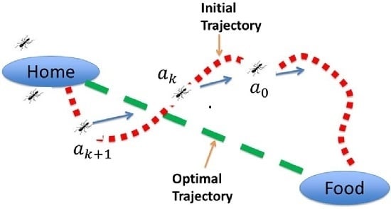
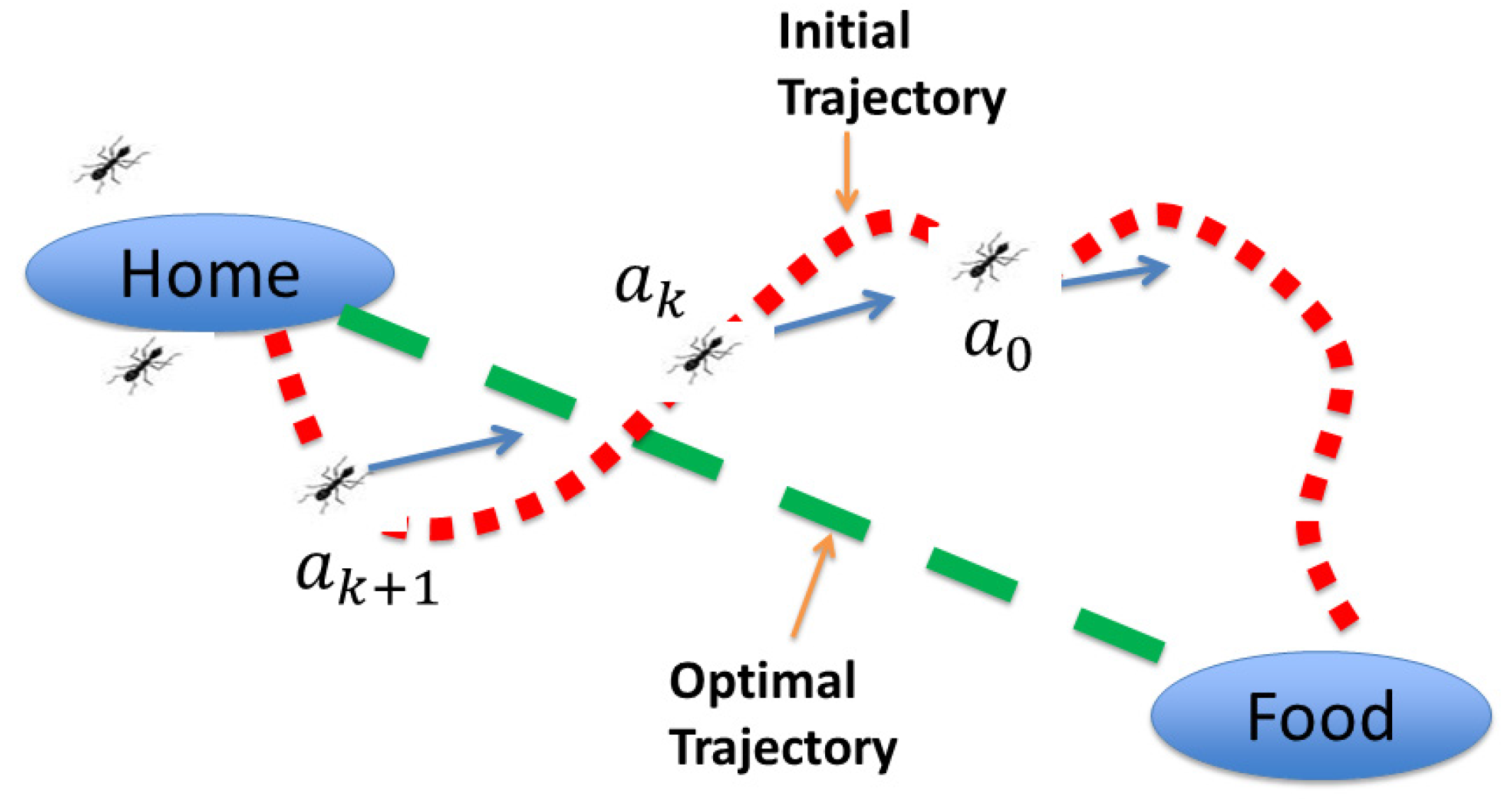
  29. Bruckstein, A.M. Why the Ant Trails Look So Straight and Nice. Math. Intell. 1993, 15, 59–62. [Google Scholar] [CrossRef]
  30. Humphrey, A.E. Fermentation Process Modeling: An Overview. Ann. N.Y. Acad. Sci. 1979, 326, 17–33. [Google Scholar] [CrossRef]
  31. Ghommidh, C.; Vaija, J.; Bolarinwa, S.; Navarro, J. Oscillatory Behaviour Ofzymomonas in Continuous Cultures: A Simple Stochastic Model. Biotechnol. Lett. 1989, 11, 659–664. [Google Scholar] [CrossRef]
  32. Jarzębski, A.B. Modelling of Oscillatory Behaviour in Continuous Ethanol Fermentation. Biotechnol. Lett. 1992, 14, 137–142. [Google Scholar] [CrossRef]
  33. Daugulis, A.J.; McLellan, P.J.; Li, J. Experimental Investigation and Modeling of Oscillatory Behavior in the Continuous Culture of Zymomonas Mobilis. Biotechnol. Bioeng. 1997, 56, 99–105. [Google Scholar] [CrossRef]
  34. Jöbses, I.M.L.; Egberts, G.T.C.; Luyben, K.C.A.M.; Roels, J.A. Fermentation Kinetics of Zymomonas Mobilis at High Ethanol Concentrations: Oscillations in Continuous Cultures. Biotechnol. Bioeng. 1986, 28, 868–877. [Google Scholar] [CrossRef] [PubMed]
  35. Jöbses, I.M.L.; Roels, J.A. The Inhibition of the Maximum Specific Growth and Fermentation Rate of Zymomonas Mobilis by Ethanol. Biotechnol. Bioeng. 1986, 28, 554–563. [Google Scholar] [CrossRef] [PubMed]
  36. Pirt, S. The Maintenance Energy of Bacteria in Growing Cultures. Proc. R. Soc. Lond. B: Biol. Sci. 1965, 163, 224–231. [Google Scholar] [CrossRef]
  37. Huang, S.Y.; Chen, J.C. Analysis of the Kinetics of Ethanol Fermentation with Zymomonas-Mobilis Considering Temperature Effect. Enzyme Microb. Technol. 1988, 10, 431–439. [Google Scholar] [CrossRef]
  38. Mahecha-Botero, A.; Garhyan, P.; Elnashaie, S.S.E.H. Non-Linear Characteristics of a Membrane Fermentor for Ethanol Production and Their Implications. Nonlinear Anal. Real Word Appl. 2006, 7, 432–457. [Google Scholar] [CrossRef]
  39. Wang, H.; Zhang, N.; Qiu, T.; Zhao, J.; He, X.; Chen, B. Analysis of Hopf Points for a Zymomonas Mobilis Continuous Fermentation Process Producing Ethanol. Ind. Eng. Chem. Res. 2013, 52, 1645–1655. [Google Scholar] [CrossRef]
  40. Georges, B.; Dochain, D. On-Line Estimation and Adaptive Control of Bioreactors; Elsevier: New York, NY, USA, 1990. [Google Scholar]
Figure 1. Framework for performing a life cycle analysis of a chemical product.
Processes 04 00023 g001
Figure 2. Schematic representation of the ant’s rule of pursuit.
Processes 04 00023 g002
Figure 3. General structure of the algorithm for the advanced control approach [27]. CL: control law; OCP: optimal control problem.
Processes 04 00023 g003
Figure 4. Schematic diagram of the fermentation reactor.
Processes 04 00023 g004
Figure 5. Open-loop simulations: concentration profiles of key component (a), biomass (b), substrate (c) and product in the fermentor (d), the membrane side (e) and the temperature profile (f) for different D m , i n values.
Processes 04 00023 g005
Figure 6. Closed-loop simulation profiles (Case 1): concentrations (a), Dm,in (b), temperatures of the fermentor and jacket (c) and Dj (d).
Processes 04 00023 g006
Figure 7. Radar plot with GREENSCOPE (Gauging Reaction Effectiveness for the ENvironmental Sustainability of Chemistries with a multi-Objective Process Evaluator) indicators for the closed-loop and open-loop simulations (Case 1).
Processes 04 00023 g007
Figure 8. Closed-loop simulation profiles (Case 2): concentrations (a), Dm,in (b), temperatures of the fermentor and jacket (c) and Dj (d).
Processes 04 00023 g008aProcesses 04 00023 g008b
Figure 9. Radar plot with GREENSCOPE indicators for the closed-loop and open-loop simulations (Case 2).
Processes 04 00023 g009
Figure 10. Closed-loop simulation profiles (Case 3): concentrations (a), Dm,in (b), temperatures of the fermentor and jacket (c) and Dj (d).
Processes 04 00023 g010
Figure 11. Radar plot with GREENSCOPE indicators for closed-loop simulations with different D i n (Case 3).
Processes 04 00023 g011
Figure 12. Closed-loop simulation profiles (Case 4): concentrations (a), Dm,in (b), temperatures of the fermentor and jacket (c) and Dj (d).
Processes 04 00023 g012aProcesses 04 00023 g012b
Figure 13. Radar plot with GREENSCOPE indicators for the closed-loop and open-loop simulations (Case 4).
Processes 04 00023 g013
Table 1. Parameter values for the fermentation process model.
A1 = 0.6225KS = 0.5 kg/m3
A2 = 0.000646KT = 360 kJ/(m2∙K∙h)
AT = 0.06 m2ms = 2.16 kg/(kg∙h)
AM = 0.24 m2mP = 1.1 kg/(kg∙h)
Ce,0 = 0 kg/m3P=4.54
Cx,0 = 0 kg/m3PM = 0.1283 m/h
CS,0 = 150.3 kg/m3VF = 0.003 m3
CP,0 = 0 kg/m3VM =0.0003 m3
CPM,0 = 0 kg/m3Vj = 0.00006 m3
cp,r = 4.18 kJ/(kg∙K)Ysx = 0.0244498 kg/kg
cp,w = 4.18 kJ/(kg∙K)YPx = 0.0526315 kg/kg
Ea1 = 55 kJ/molTin = 30 °C
Ea2 = 220 kJ/molTw,in = 25 °C
k1 = 16.0 h−1H = 220 kJ/mol
k2 = 0.497 m3/(kg∙h)ρr = 1080 kg/m3
k3 = 0.00383 m6/(kg2∙h)ρw = 1000 kg/m3

