Incorporating Enhanced Decision-Making Capabilities into a Hybrid Simulator for Scheduling of Batch Processes

Abstract

A simulation model can accurately capture the details of product recipes in a batch process. By incorporating enhanced capabilities for making key assignment decisions in the simulation executive a model can mimic the experiential knowledge and rules employed in operating a process. As the process complexity and problem size increase using the mathematical programming (MP) techniques to generate schedules becomes increasingly difficult. A simulation run typically takes very little computation time and generates a schedule that is verifiable. Moreover, the model can be used to explore a wide range of parametric space to evaluate alternate policies and the impact of process uncertainties. Although there is no guarantee of optimality, the quality of schedules thus generated is very good and can be deployed in operations. In this paper the decision-making capabilities of the BATCHES simulator are presented with its application to a set of scheduling problems reported extensively in the literature. The results show that ‘smart’ simulation can be used effectively for a large set of scheduling problems.

1. Introduction

A schedule predicts the start and end times, and in some cases the batch size, of each task processed on each piece of equipment in a process for the specified performance measures used in creating that schedule. Often the actual start and end times do not match exactly with the predicted values because of process uncertainties. Typically, a schedule is used as a guide by plant operations personnel who adhere to the sequence of tasks. If the process starts deviating from the predicted schedule, at some point it becomes necessary to generate a new schedule or to undertake an ad hoc adjustment.

Scheduling is critical in improving the productivity of multiproduct and multipurpose batch processes. Over the past 30 years, the scheduling problem has been studied extensively in academia and industry, and across a range of industry sectors such as discrete manufacturing and process industries [1,2,3]. A significant portion of the past work uses mixed integer programming (MIP) for solving the scheduling problem using discrete-time or continuous-time formulation. Although the MIP-based methods guarantee optimality, often the underlying process is simplified so that the problem can be solved in a reasonable amount of time. Some of the inherent complexities simply cannot be handled, such as uncertainties in parameters, while some simplifications are necessary in order to control the problem size, such as the granularity of the discrete time.

Additionally, the scheduling applications can be broadly divided into two categories, off-line or real-time. Typically, in off-line applications the time available to find a solution can be fairly large, of the order of several hours or days. The real-time scheduling problems often arise due to the need to modify or reschedule a previously-generated schedule in order to compensate for the deviations in the actual process trajectory. The time available for solving the real-time, rescheduling problems is often very limited, of the order of an hour or less. In such cases, mathematical programming (MP)-based formulations may not be able to provide timely solutions.

The limitations of mathematical programming techniques in handling complexities and providing timely solutions provide an opportunity to apply other techniques, such as simulation-based methodologies. Simulation has been used extensively in designing batch processes [4,5]. However, simulation has not been extensively used in addressing scheduling problems, mainly because of the inherently myopic view that this technique takes in making assignment decisions. Thus, at any point in time when a simulator has to decide whether to assign a particular piece of equipment to perform a particular task, it has knowledge only of the current state of the process and has no mechanism to evaluate a priori the impact of the decision on a global performance measure, such as an objective function. Such a mechanism would provide the criteria for making or not making a certain decision which, in turn, would affect the schedule. Simulation, coupled with heuristics, has been applied to discrete systems. However, in general the characteristics of batch processes are very complex compared to discrete systems. The complexities preclude the use of discrete event simulation based systems in applications related to batch processes. A simulation-based framework applied to batch processes, as reported by Chu et al. [6,7], augments the underlying MP-based formulations, and has similar limitations as stated earlier.

The following are some of the commercially available simulators for batch processes: Batch Process Developer [8], suite of products by Intelligen, Inc. [9], gPROMS [10], and BATCHES [11]. DynoChem [12] is designed for simulating single unit operations used in batch processes. None of these simulators, other than BATCHES, has the ability to dynamically assign a task to a piece of equipment, a key functionality required for solving scheduling problem. The BATCHES simulator [12,13] will be used for solving the scheduling problems discussed in this paper.

One of the key steps in the formulation of scheduling problems for batch processes is the modeling of the underlying recipes. The state-task network (STN) [14] or a more generalized resource-task network (RTN) [15] is often used by the MP-based frameworks to model recipes. BATCHES provides modeling constructs that are similar to ANSI/ISA-88 standards [16] to model recipes of various products. These constructs, discussed later, allow very detailed recipe specifications to be incorporated into a model. In addition, the simulator uses a combined discrete and dynamic simulation executive which was developed specifically to meet the special needs of multiproduct and multipurpose batch processes. New capabilities to facilitate improved assignment decisions have been added to the simulator with the view of addressing scheduling problems.

In this paper we demonstrate the use of the simulation methodology of BATCHES to solve a set of five scheduling problems which has been studied extensively in the literature. Some of the problems have been modified to suit the limitations of the simulation technique. As we observed for this limited set of problems the simulation method provides very good, sometimes identical results, within a small fraction of computation time. The objective of the paper is not to use simulation for each formulation discussed in the literature, but merely to demonstrate that simulation is a viable technique for solving scheduling problems. Therefore, a set of five representative problems was selected from the literature to illustrate specific capabilities of the BATCHES simulator. The details of the MP formulations and descriptions of underlying process for these examples are available in the paper by Susarla et al. [17].

In the first two sections, the key differences in building process models and the approach to solving scheduling problem using the simulation and mathematical programming techniques are discussed. The subsequent sections compare the results for the five examples from the literature. In the description, the word “simulator” implies the BATCHES simulator.

2. Process Modeling

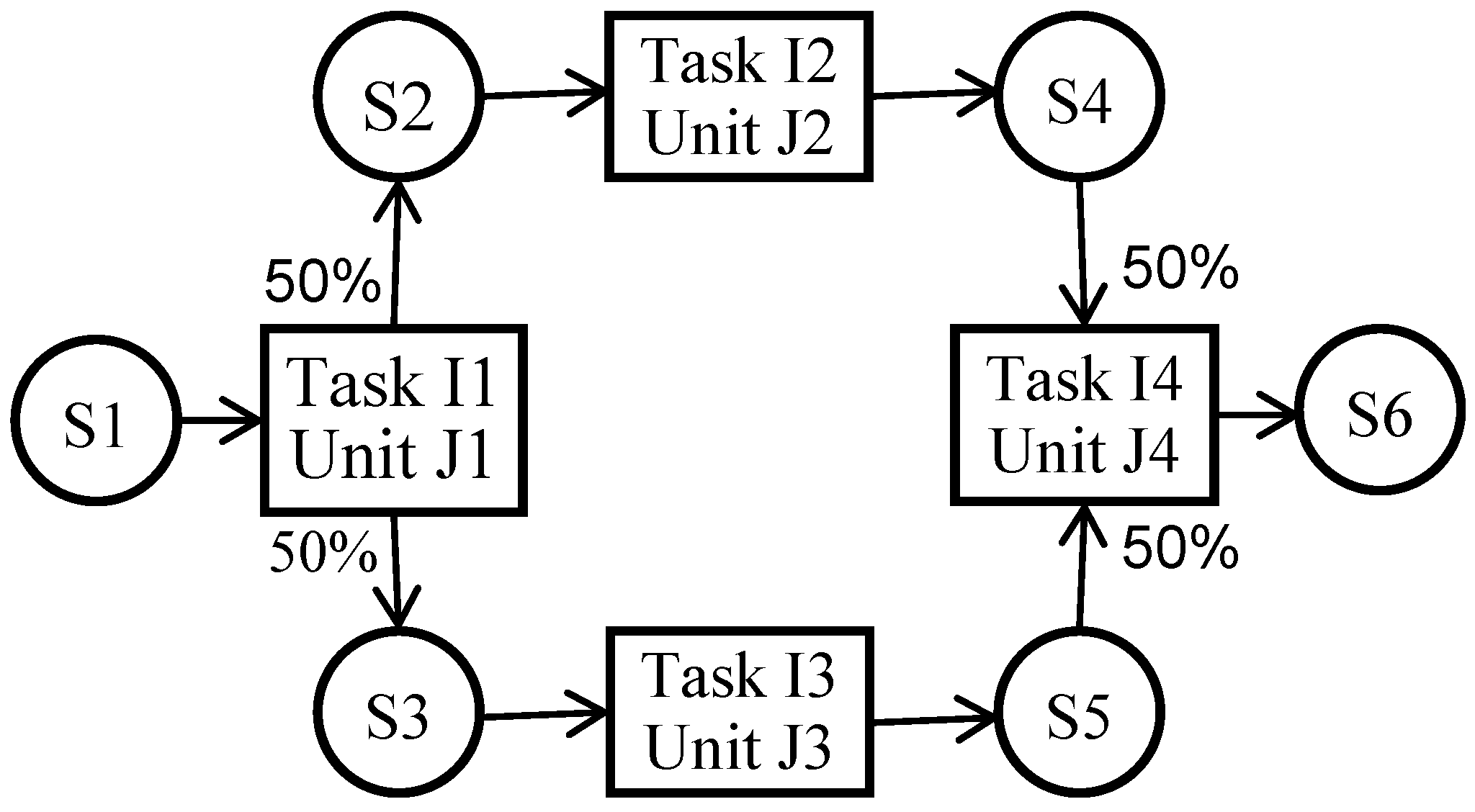
The mathematical programming formulations of the problems considered in this paper use state-task networks to model the process recipes. As an example, the STN for the recipe used in Example 1 (discussed later) is shown in Figure 1. In general, a STN consists of tasks with material storage states upstream and downstream of each task. The tasks model the transformations and account for the processing times. Most of the times the transfer of material between a storage state and task is assumed to be instantaneous. As shown in Figure 1, a batch of task I1 is split in half and goes to states S2 and S3, while materials from states S4 and S5 are mixed in equal proportions to make a batch of task I4. A dedicated piece of equipment is available to perform each task. In the MP formulations storage states are influenced by a storage policy associated with each state. The policies typically used are unlimited intermediate storage (UIS), limited intermediate storage (LIS), no intermediate storage (NIS), unlimited wait (UW), limited wait (LW), and zero wait (ZW). For the UIS and LIS policies, a physical unit(s) is(are) available in the process, while for the UW, LW, and ZW policies the material is typically held in the upstream equipment until it can be emptied downstream in a suitable unit.

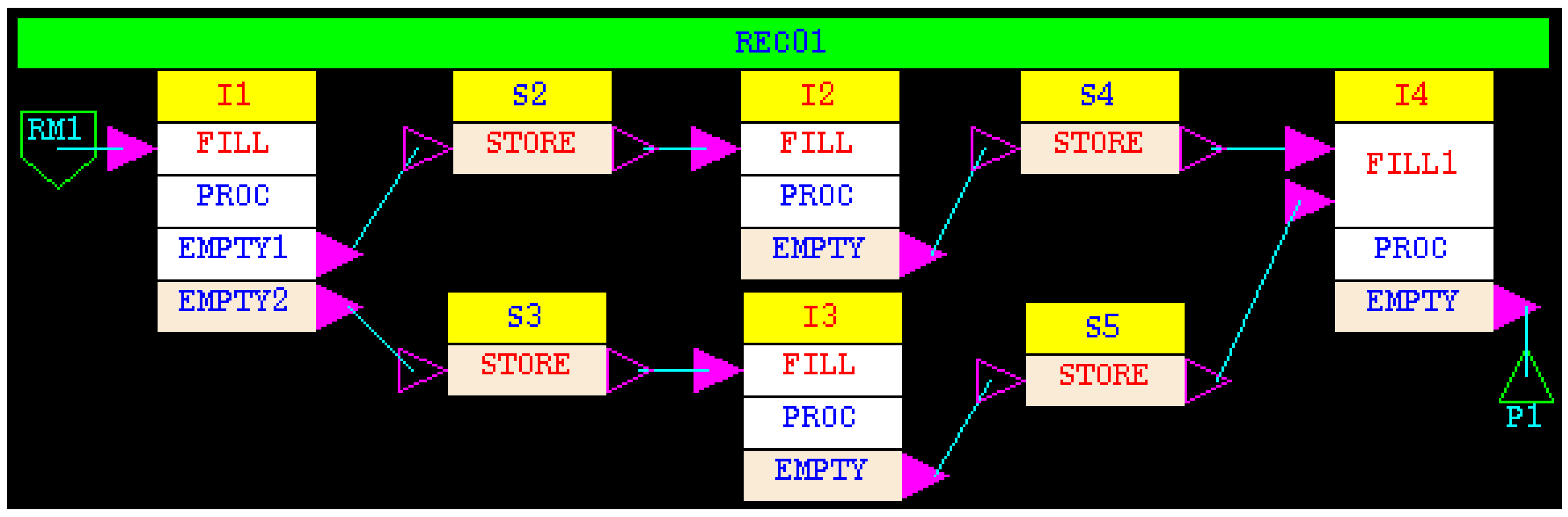
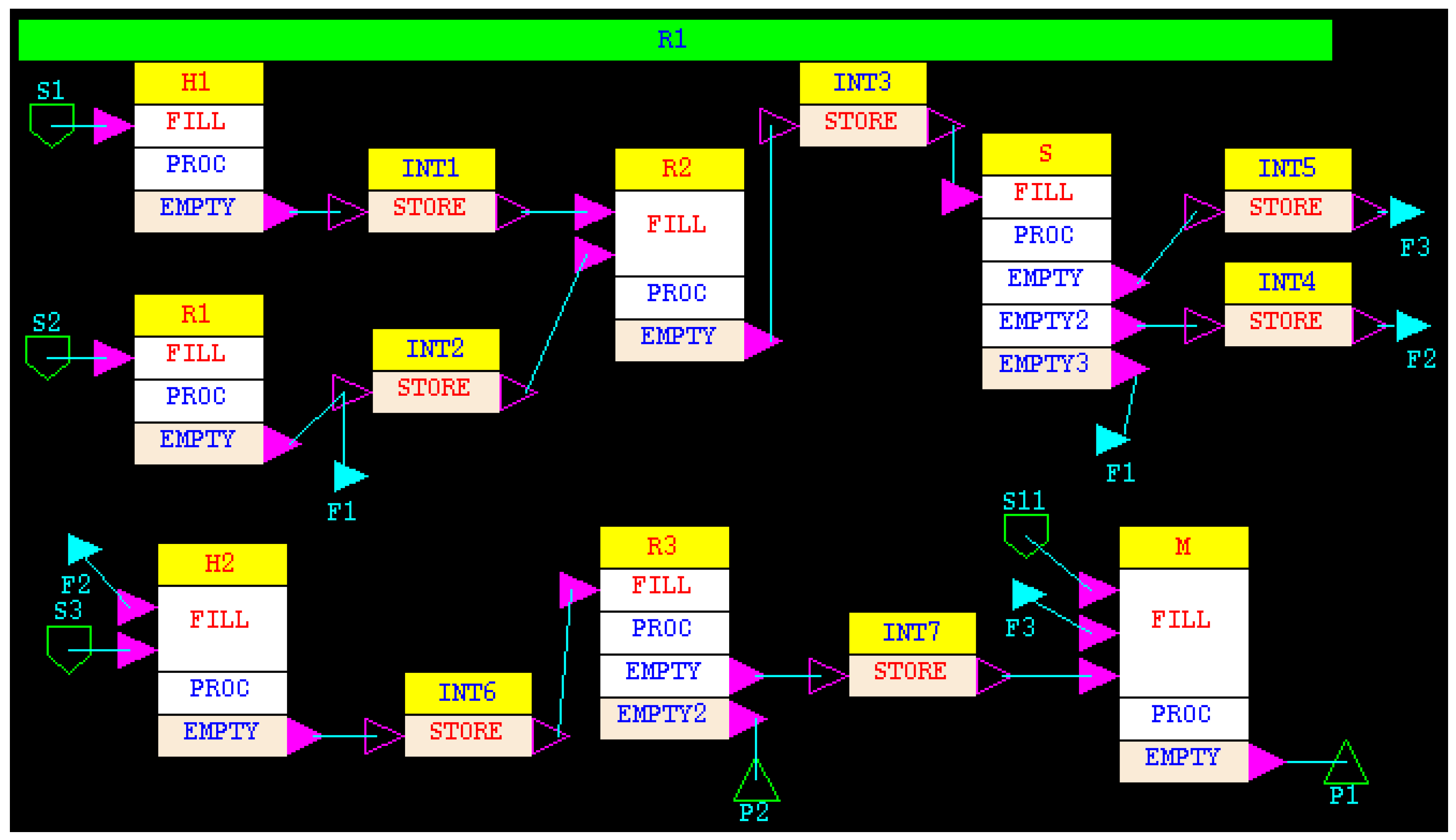
In the simulation model, a recipe is modeled as a recipe network and the processing units are modeled as an equipment network. A recipe consists of tasks and each task, in turn, consists of subtask(s). Each task in a STN has a corresponding task in the recipe network. In addition, for a physical storage tank, which exists when the storage policy is UIS or LIS, there is a corresponding task in the recipe network. The recipe network shown in Figure 2 is used for modeling the STN shown in Figure 1 with physical storage tank. A task in the STN is modeled as a series of three subtasks, FILL, PROC, and EMPTY to represent the three separate steps during the execution of a task, namely filling, processing, and emptying. If a batch is split multiple ways, there is an emptying subtask for each split. Similarly, if materials from more than one upstream states are mixed, then the filling subtask has corresponding number of inputs. Of course, the duration associated with each transfer is zero, while the duration of the PROC subtask corresponds to the task duration. The storage task which models the UIS or LIS policy is modeled as consisting of one subtask with decoupled input and output (hollow input and output symbols on subtask STORE). Thus, tasks S2, S3, S4, and S5 in Figure 2 correspond to the storage states S2, S3, S4, and S5 in the STN shown in Figure 1. Raw material RM1 represents state S1, indicating material is always available. Sink P1 represents state S6, indicating that material can be emptied at any time subtask EMPTY of task I4 starts. The NIS, UW, LW, and ZW policies are modeled naturally in the recipe network by not having a storage task. For example, if there is no intermediate storage after task I3, the output from the EMPTY subtask would go directly to the FILL subtask of I4. However, in STN such storage states are artefacts of the associated framework. Thus, a recipe network represents the actual process recipe more accurately.

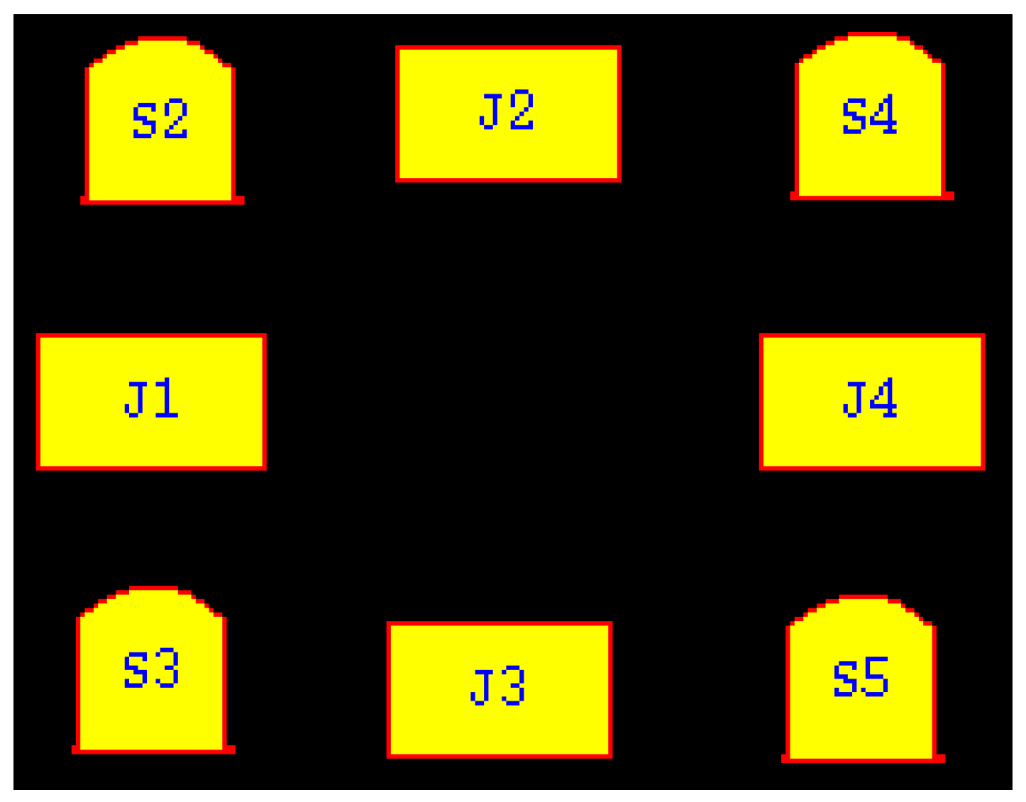
The equipment network for Example 1 is shown in Figure 3. In this example, for each storage state and ‘process’ task of the STN, there is one piece of equipment in the equipment network. The equipment parameters such as volume are specified in the equipment network. In addition any connectivity constraints are also shown graphically in the equipment network. When there are no connectivity constraints, the equipment network is merely a set of icons representing the units in a given process, for example, the equipment network in Figure 3. For each task in a recipe network there is at least one unit suitable to perform that task. In multipurpose processes, a unit or a set of parallel units can be used for performing multiple tasks. In such cases, the tasks that are performed on those units have the same list of suitable units.

The GUI of the simulator is used for building the equipment and recipe networks.

2.1. Making a Simulation Run

A task in a recipe can either be an independent task or a dependent task. If an input to a task pulls upstream material, such as from a raw material or a storage state, then it is an independent task. An input that pulls material is displayed as a solid triangle in the recipe network. If an upstream output pushes material into a task, the receiving task is a dependent task. An input that accepts pushed material is displayed as a hollow triangle in the recipe network.

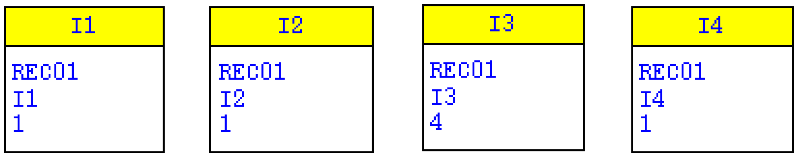
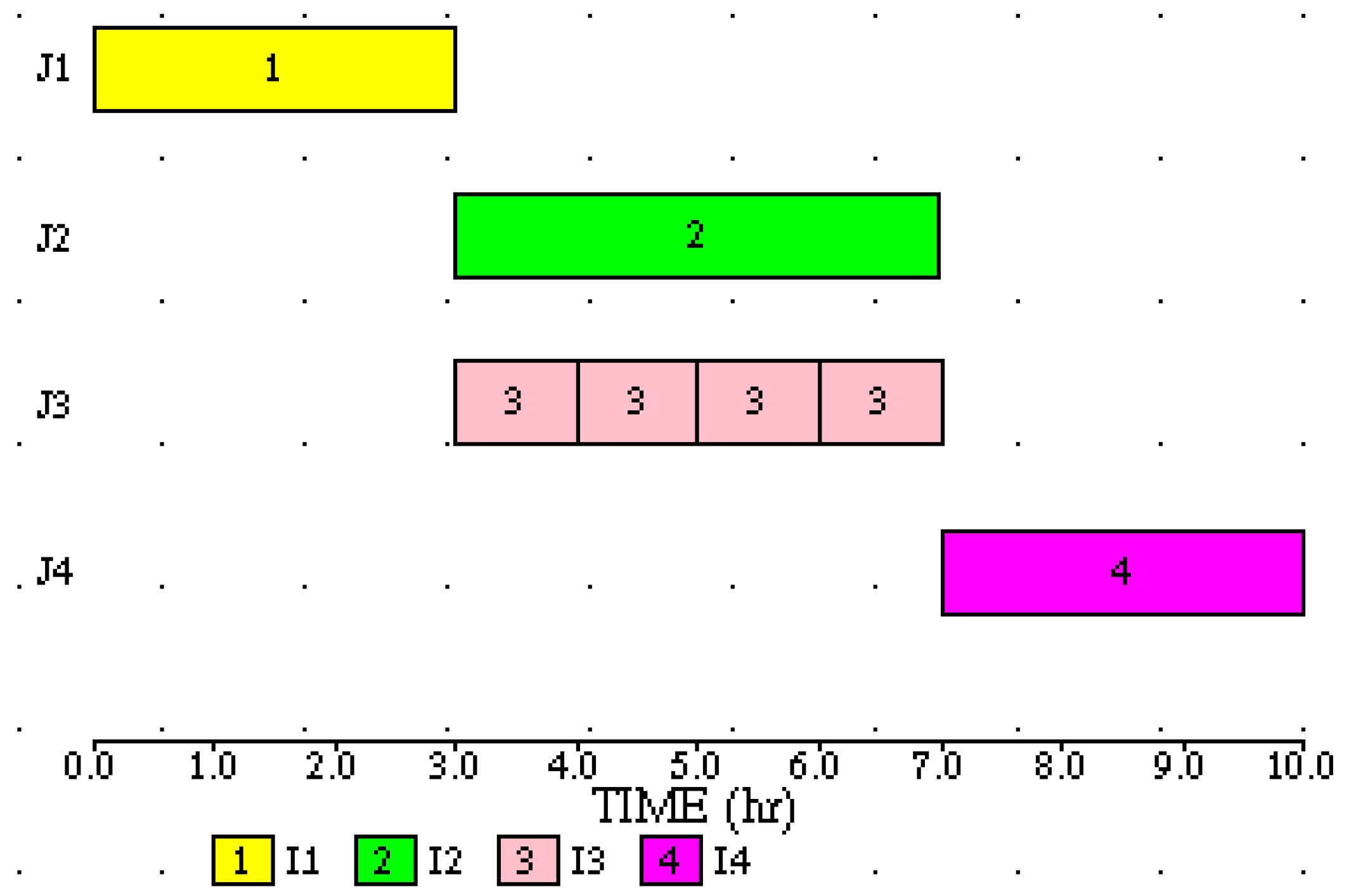
In simulation, processing directives are used for initiating independent tasks. As the name suggests, the processing directives broadly define how much material should be produced or how many batches of independent tasks should be initiated. For example, for the recipe shown in Figure 2 the simplest processing directive would be “Make n batches of task I1 of recipe REC01”. Note that I2, I3, and I4 are also independent tasks because they pull material from upstream storage tasks. Thus, processing directives must be specified for initiating those tasks. Four processing directives for starting the four tasks are shown in Figure 4. Each directive (yellow box) has the time at which it starts, and individual directives act in parallel. An entry in a processing directive (white box) identifies the task to be initiated and the number of batches to be produced of that task. As shown in the example, one batch each of I1, I2, and I4 is initiated, and four batches of I3 are initiated. A task is assigned to a unit only if it is available at a given time and the specified amount of material is available in an upstream unit.

As the simulation marches in time, the assignments of units to the independent tasks are made through the processing directives. The assignments to dependent tasks are made through queues of requests created by upstream subtasks pushing material downstream. Once a task is assigned to a unit, its execution is governed by the specified recipe.

The key results generated during a simulation run are the material balance, equipment utilization and the Gantt chart. Of course, a Gantt chart is the schedule created by the simulator.

One of the input parameters for a simulation run is the end of simulation time. If the simulation end time is too large, all the required number of batches are completed before the end time, and the result of interest is the makespan, that is, the time required to process the specified batches. If the end time is the intended scheduling time horizon, for example, one day, then the result of interest is the amount produced in the specified time.

2.2. Quality of Schedule

Typically, for scheduling applications the desired time horizon is specified for a simulation run, such as one day or one week. If the selling price, in $/kg, for each of the useful product streams, and processing cost, in $/kg, for each of the waste streams is provided, the simulator computes the total revenues for a run. In addition, if the usage costs for all the resources are provided, such as $/h for each equipment, operator, and utility and $/kg for each raw material, then the simulator also computes the total profit for a run. Furthermore, by using activity based costing the simulator calculates profit/kg for each product. Thus, total profit for a simulation run becomes the key performance measure to evaluate the quality of schedule it generates. In the absence of costing data total amount of useful products and waste streams produced are used to evaluate the schedule quality. Often, the optimization formulations use profit as the objective function.

A good measure of the quality of a schedule is the utilization of resources, typically equipment. If a stage in a process is utilized close to 100% then most likely there is no slack available in the process, and the amount produced would be the maximum possible from the process. The only way to get more production would be by making modifications to the process, such as modifying cycle times or adding/deleting equipment. Of course, making process modifications is beyond the scope of scheduling problems. Often a Gantt gives a good visual confirmation of units reaching peak utilization. The simulator also generates percent utilization for each unit, which can be used as a quantitative measure of the quality of schedule.

Since optimization using simulation is an iterative process, with no guarantee of global optimum, the number of ‘what ifs’ could skyrocket depending on the parametric space to be explored. Experiential knowledge becomes crucial in limiting the search space. Often the user has a good idea about the typical sequences in which to make products, or the number of batches to initiate in order to produce the desired amount of a product, and so on. Thus, within a limited number of runs a good quality schedule can be obtained. The greatest advantage of a simulation-based approach is that the underlying process can be very accurately modeled, thereby the schedule produced will be very accurate and reliable, though not necessarily optimal.

In this paper, we have used simulation in scheduling processes for which an optimum solution has already been generated. Therefore, the quality of the simulated schedule can be easily determined by comparing it to the optimum solution. Additionally, the corresponding Gantt chart shows, visually, the quality of the simulation generated schedule.

3. Limitations of Simulation-Based Scheduling

In the MILP formulations batch size is often a decision variable with defined upper and lower bounds. It is often coupled with a linear processing time dependency, for example:

Processing time = α + β∙M

where M is the batch size and α and β are constants. This means that for each batch the amount produced, as well as duration, can be changed. Changing batch size for each batch is not impossible, but tedious to achieve in a simulation run. Typically, the size of each batch is determined by the recipe specifications. However, through processing directives it is possible to specify the size of a batch, overriding the recipe. This is equivalent to specifying the start time and batch size for each batch initiated through processing directives. This amounts to specifying the schedule and using the simulator to test if it will work. In typical scheduling applications, the simulator should generate the start time (the schedule) for each batch on each piece of equipment based on the recipe specifications.

For the linear processing time dependency the average throughput of a unit or a stage, given by M/(α + β∙M), is maximum when M is maximum, or at the upper bound. Thus, by producing batches of sizes smaller than the maximum possible size, the throughput of a stage or the process itself could be reduced. This is typically justifiable only to exploit short-term scheduling.

During simulation, unless modified through processing directives, the batch sizes can be computed to fully occupy the available unit. Therefore, if the units suitable for a task have different sizes, the amount of material and the cycle times for that task in each unit would be different. Therefore, simulation should be used with caution for short-term scheduling and the possibility of changing the batch sizes should also be considered.

During plant operation, changing the size of each batch is difficult to implement due to practical considerations. Normally, the operating recipes, particularly batch size, are not altered on the fly because that could potentially affect numerous operating parameters and may result in previously unknown trajectories and deviations, and some time in failed batches. For simple tasks, such as mixing, it may be feasible to change batch sizes on the fly without significantly affecting the overall process.

4. Enhanced Decision-Making Capabilities of the Simulator

The simulator uses the combined discrete and dynamic methodology to march in time. The trajectory of a process is marked by points in time at which the state of the process changes instantaneously, called discontinuities. Between discontinuities the simulator solves the set of differential/algebraic equations associated with the process dynamics models that best describes the physical/chemical change taking place in the subtasks of all active units. A state variable associated with a dynamics model can be used to define a state event condition. A state event is triggered when a certain variable crosses a specified threshold in a particular direction. The time of occurrence of a state event is not known a priori. For the other type of events, called time events, the time of occurrence is known a priori. At each discontinuity, marked by one or multiple events occurring at that time, the simulation executive scans through all processing directives currently active to decide whether any idle unit can be assigned to perform specified tasks. Note that a sequence of tasks to be initiated is specified in a directive, and each task, in turn, has a list of suitable units. The following functionalities are available in the simulator to solve scheduling problems presented in this paper: equipment assignment logic option, size-dependent material requirements, and queue priorities. These functionalities are discussed in the following sections.

4.1. Equipment Assignment Logic Option

By default the assignment of equipment to a task is made strictly based on the availability of a piece of equipment. Such an assignment logic is very myopic and greedy. Once a unit is assigned to a task it is released only after the assigned task is completed. Thus, if material is not available for the assigned task, the unit must wait until the material becomes available. Moreover, when it is assigned to a task, the unit cannot be assigned to any other task.

An alternative assignment logic option is available, which if specified, requires the executive to perform additional checks prior to assigning equipment to a task. This option stipulates that a piece of equipment should be assigned only if it is available and sufficient material is available upstream to fulfil the material requirement specifications for all inputs to the filling subtask. This option plays an important role when parallel units have different sizes and when multiple tasks are competing for the same set of units. For example, suppose unit A1 needs 100 kg and a parallel unit A2 needs 75 kg to fill. If both A1 and A2 are idle at a given time, but only 75 kg is available upstream, then the simulator will assign unit A2 if the new logic is specified in the recipe model. Using the default logic it would assign unit A1 and wait until the additional 25 kg becomes available upstream.

4.2. Size Dependent Material Requirement

For a subtask that pulls upstream material the simulator provides a range of options to determine how much material to pull, for example, specified mass or a specified fraction (1 means entire upstream batch). To accommodate the possibility that the downstream equipment items could be of different size and as a consequence the material required may depend of the equipment assigned to the task, an additional option for material specification is available. This option, if selected, directs the simulation executive to compute the mass required based on equipment volume and material density. As explained above, the new material specification coupled with the new assignment logic option can result in improved assignment decisions.

4.3. Queue Priorities

In the simplest case, the requests for assigning a unit to a task generated through processing directives are kept as an ordered list in a queue using the first-in-first-out (FIFO) rule. The FIFO rule can be improved through the specification of priority, a positive integer, associated with a processing directive entry. The primary queuing criterion is based on the priorities, and within the same priority the FIFO rule is used. Thus, the higher the priority, the closer to the top of the queue the associated request is placed. At each discontinuity, the simulation executive reviews the entries in each queue, beginning with the top entry, to determine whether a unit could be assigned to the task associated with each entry. Typically, a set of parallel units has one queue associated with it, and all requests for tasks which can be performed on that set reside in that queue.

The priorities play a crucial role in determining the order of unit assignment, particularly when a set of parallel units is suitable for multiple tasks, typical of multipurpose processes. As a general guideline, the priority of a task which is downstream of a competing task should be higher. The rationale being that if the downstream material is not processed then it could potentially back up a process. Therefore, if material is available to perform two tasks that can be performed on a unit that is available at a given time, then it would be assigned first to the task with higher priority (the downstream task). Intuitively, the use of priorities for conflict resolution is similar to the logic that might be used in practice.

5. Scheduling Examples

In this Section five processes used for testing various MP-based formulations of scheduling problems are discussed. For each process there may be several formulations based on storage policy, operating policy and so on. Collectively there are more than 30 published papers addressing the scheduling of these five processes. The intent of this paper is to illustrate the use of simulation in scheduling these processes. Therefore, the results for only one sample case for each process are presented. For the ease of comparison, we have chosen those cases for which Gantt charts have been shown in the paper by Susarla et al. [17]. The headings in this section match with the section headings in the reference. References to other works are also available in the paper by Susarla et al. [17].

To save space, only the recipe diagrams of the processes are given in various figures. The STNs are given in the Susarla paper [17]. The task and storage states in an STN have tasks with same names in the recipe network. Additionally, in all examples default equipment networks are used, that is, one icon for each unit and no connectivity constraints. The figures of equipment network are not given in the paper. The UIS storage policy is used in the simulation.

The simulation runs were made on an HP 15 TouchSmart laptop, IntelCore [email protected] GHz processor, running the Ubuntu 12.04 64-bit operating system.

5.1. Example 1

The STN and recipe network for this example are shown in Figure 1 and Figure 2. The key process parameters are given in

Table 1. Key process parameters for Example 1.

Task	Unit	α	β	M, kg
I1	J1	1.666	0.03335	40
I2	J2	2.333	0.08335	20
I3	J3	0.667	0.0666	5
I4	J4	2.667	0.00833	40

. A batch of task I1 is split in half and sent to the storage states.

Processing directives were set to make one batch each of tasks I1, I2, and I4, and four batches of I3 because each batch of I1 results in four batches of I3. All four batches of I3 and a batch of I2 are needed to make a batch of I4.

A time horizon of 10.0 h is specified for the simulation run.

In the specified time horizon 40 kg P1 is produced, which is the same as the amount produced by the best solution using MP. The task-based Gantt chart for the simulation run is shown in Figure 5. The traces of levels in storage units show that they lie within the specified bounds.

The simulation run took 0.031 s (user + sys values from the Linux time command). The CPU times for the MILP formulations for this problem are not reported.

The Gantt chart shows that it is not possible to produce any more material in the specified time horizon. Therefore, this is an optimal solution confirmed. This is also confirmed by the amount produced by simulation to be the same as the amount produced by the optimal solution.

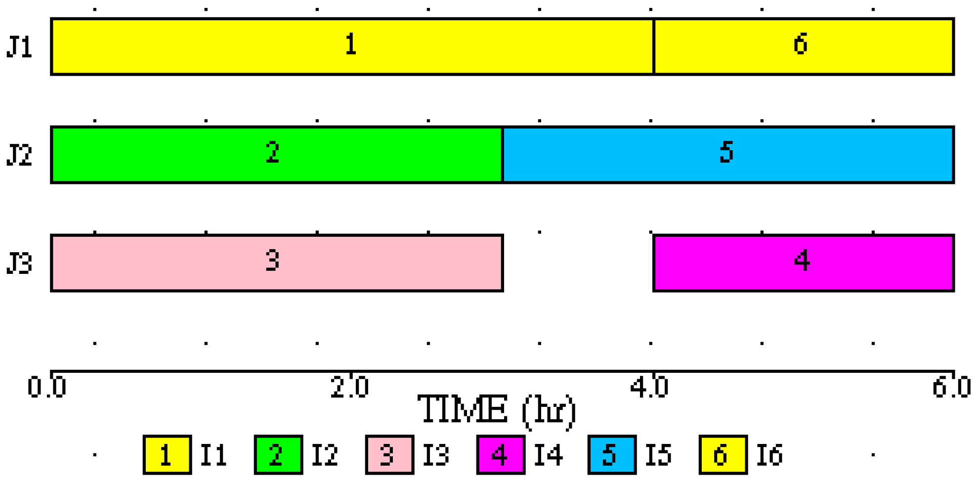
5.2. Example 2

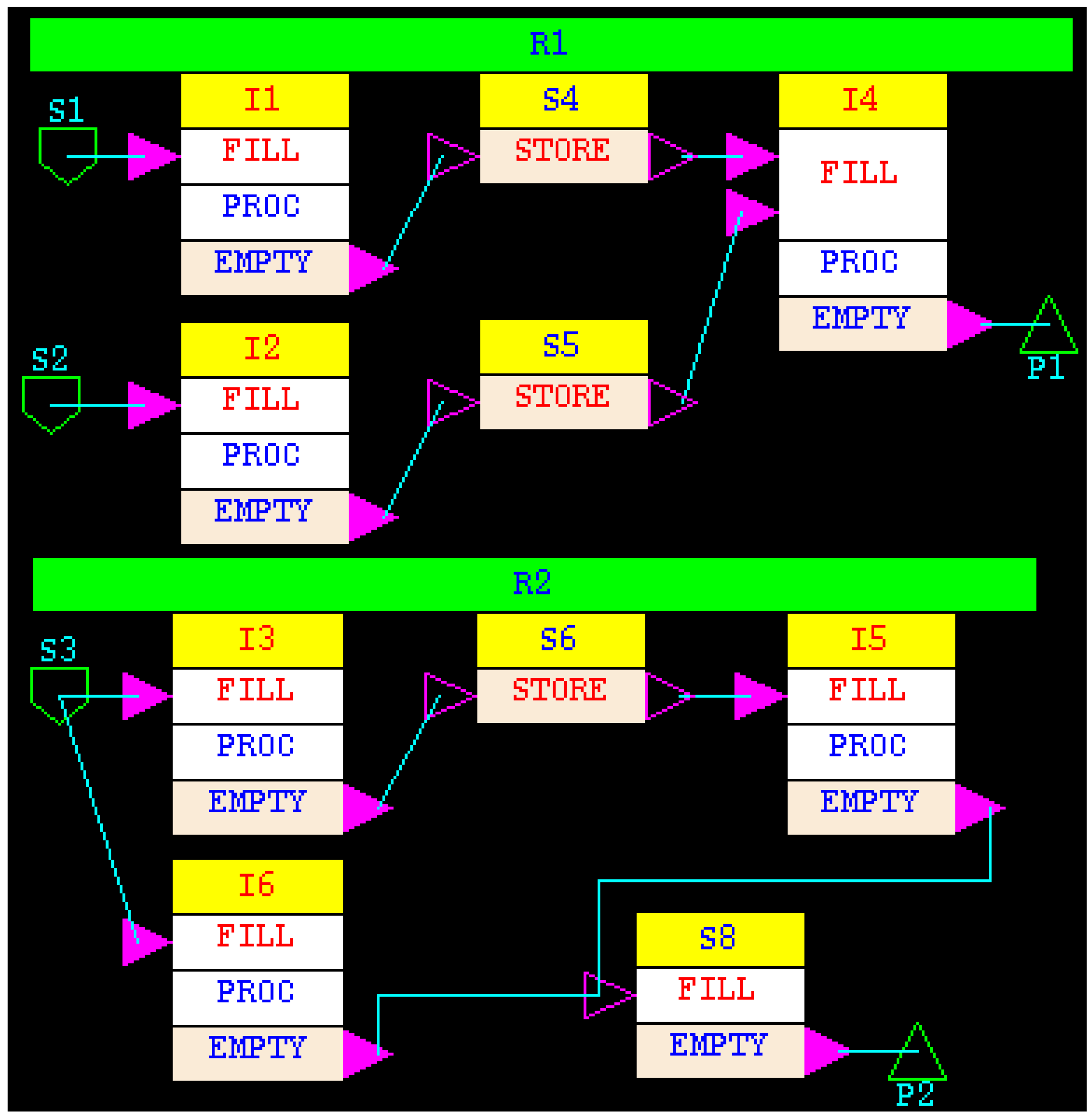
The recipe networks for this example are shown in Figure 6. The key process parameters are given in

Table 2. Key process parameters for Example 2.

Recipe	Task	Unit	α	β	M, kg
R1	I1	J1	1.666	0.0778	30
	I2	J2	2.333	0.0667	10
	I4	J3	0.667	0.0033325	40
R2	I3	J3	0.669	0.0777	30
	I5	J2	1.332	0.0556	30
	I6	J1	1.5	0.025	20

. In this process, two recipes are manufactured, producing two products P1 and P2. Each unit in the process is suitable to perform two tasks.

The two independent tasks I1 and I2 of recipe R1 are parallel so they should be started as close to each other as possible. Therefore, a priority of two was assigned to the processing directives for starting I1 and I2. Consequently, since I6 competes with I1 for unit J1, a priority of one was assigned to the processing directive for starting I6. Task I4 is a downstream task and competes with I3 for unit J3. Therefore, priorities of two and one were assigned to their respective processing directives so that I4 will get preference over I3, thereby unblocking the upstream material. Similarly, I5 is a downstream task and competes with I2 for unit J2. Therefore priority of three was assigned to I5 so that gets preference over I2. A time horizon of 6.0 h was specified for the simulation run.

In the specified time horizon, 50 kg P1 and 40 kg P2 are produced, which are the same as the amounts produced by the best solution using MP. The task-based Gantt chart for the simulation run is shown in Figure 7. The best solution using MP assumes that material in storage task S5 is allowed to flow through into task I4, thereby rendering ineffective the storage constraint, or ignoring the storage tank. Thus, task I4 would start in J3 at time 3.0 h and wait in J3 until J1 finishes I1 at time 4.0 h. One way to accomplish this in the simulation is to treat S5 as UIS, thereby releasing J2 as soon as task I2 is completed and allow material to wait in S5 until time 4.0 h. The traces of levels in storage units show that they within the specified bounds. To ignore storage, the recipe network must be modified to reflect the actual operation.

The simulation run took 0.039 s (user + sys values from the Linux time command). The CPU times for the MILP formulations for this problem are not reported.

The Gantt chart shows that there is no slack time on both J1 and J2. Therefore, it would not be possible to produce any more material, and the schedule is optimal. This is also confirmed by the amount produced by simulation of the two products to be the same as the amount produced by the optimal solution.

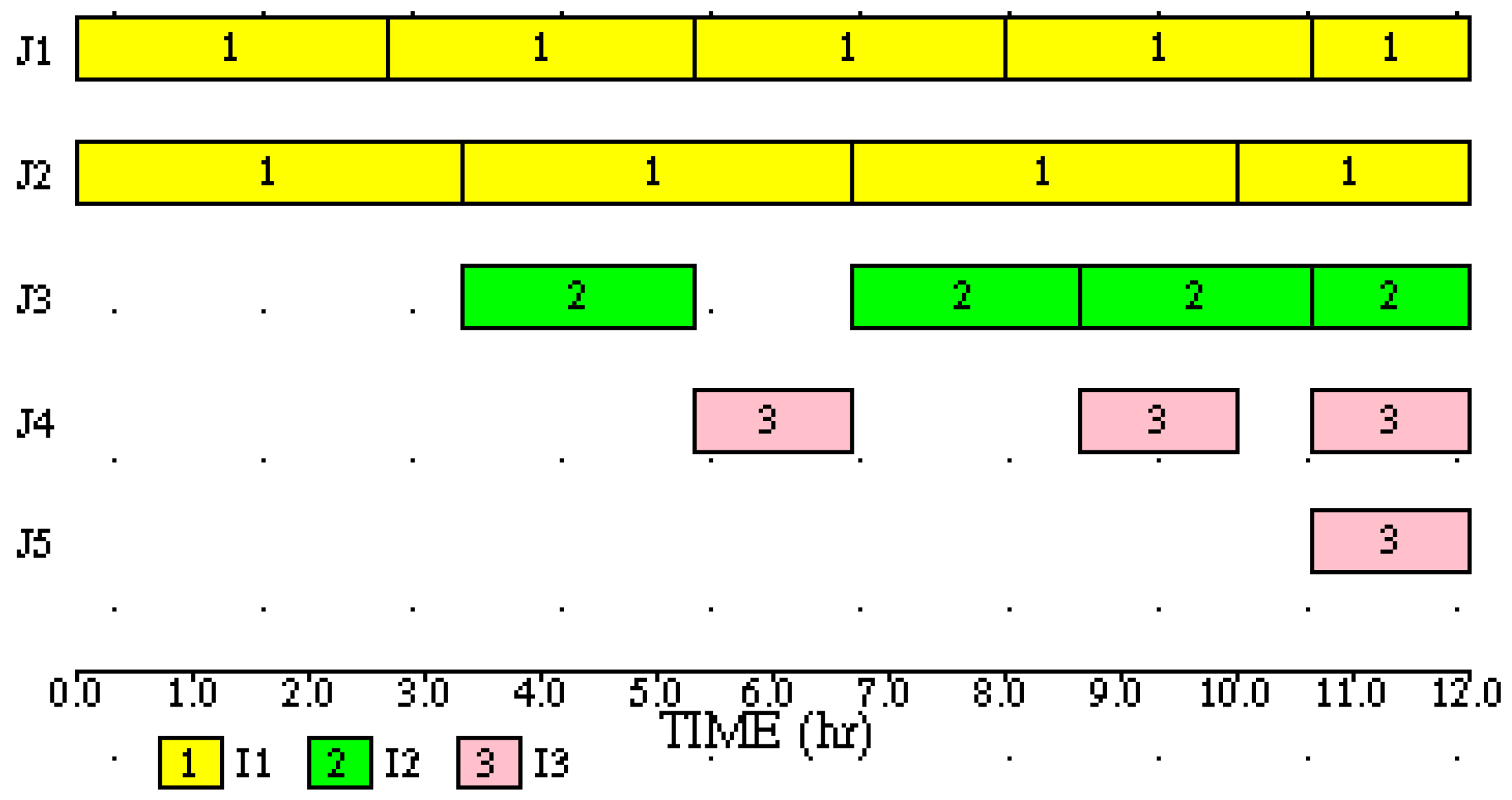
5.3. Example 3

The recipe network for this example is shown in Figure 8. The key process parameters are given in

Table 3. Key process parameters for Example 3.

Task	Unit	α	β	M, kg
I1	J1	1.333	0.01333	100
	J2	1.333	0.01333	150
I2	J3	1.0	0.005	200
I3	J4	0.667	0.00445	150
	J5	0.667	0.00445	150

. Two units are suitable to perform task I1 and two to perform task I3. The two units suitable for task I1 have different sizes. A storage tank is available between tasks I1 and I2, and another between tasks I2 and I3.

Processing directives were specified to initiate the three independent tasks I1, I2, and I3. For tasks I2 and I3, a unit was assigned only when the required amount becomes available in the upstream intermediate storage tanks. Since the input to task I1 is from a raw material, the batches in units J1 and J2 are initiated without delay. The batches in downstream stages are staggered because material is not always available to start them without delays.

A time horizon of 12.0 h was used in this example. The Gantt chart is shown in Figure 8. The schedule generated by the simulation model is similar to the optimum schedule. However, the optimizer was able to adjust batch sizes, and consequently the duration of each batch, so as to fit complete batches in the given time horizon. In the simulation, since the batch sizes could be adjusted, the total amount produced of product P1 is 600.0 kg compared to 692.665 kg in the optimum solution. However, in the simulation at the end there is 200.0 kg in equipment J3 and 50.0 kg in S2.

The simulation run took 0.045 s (user + sys values from the Linux time command). Some of the MILP formulations did not converge in 10,000 CPU s while some solutions took 5403 CPU s. The appropriate logic used to assign equipment in the simulation was sufficient to schedule this process.

The Gantt chart in Figure 9 shows that there is no slack time on both J1 and J2. Therefore, it would not be possible to produce any more material.

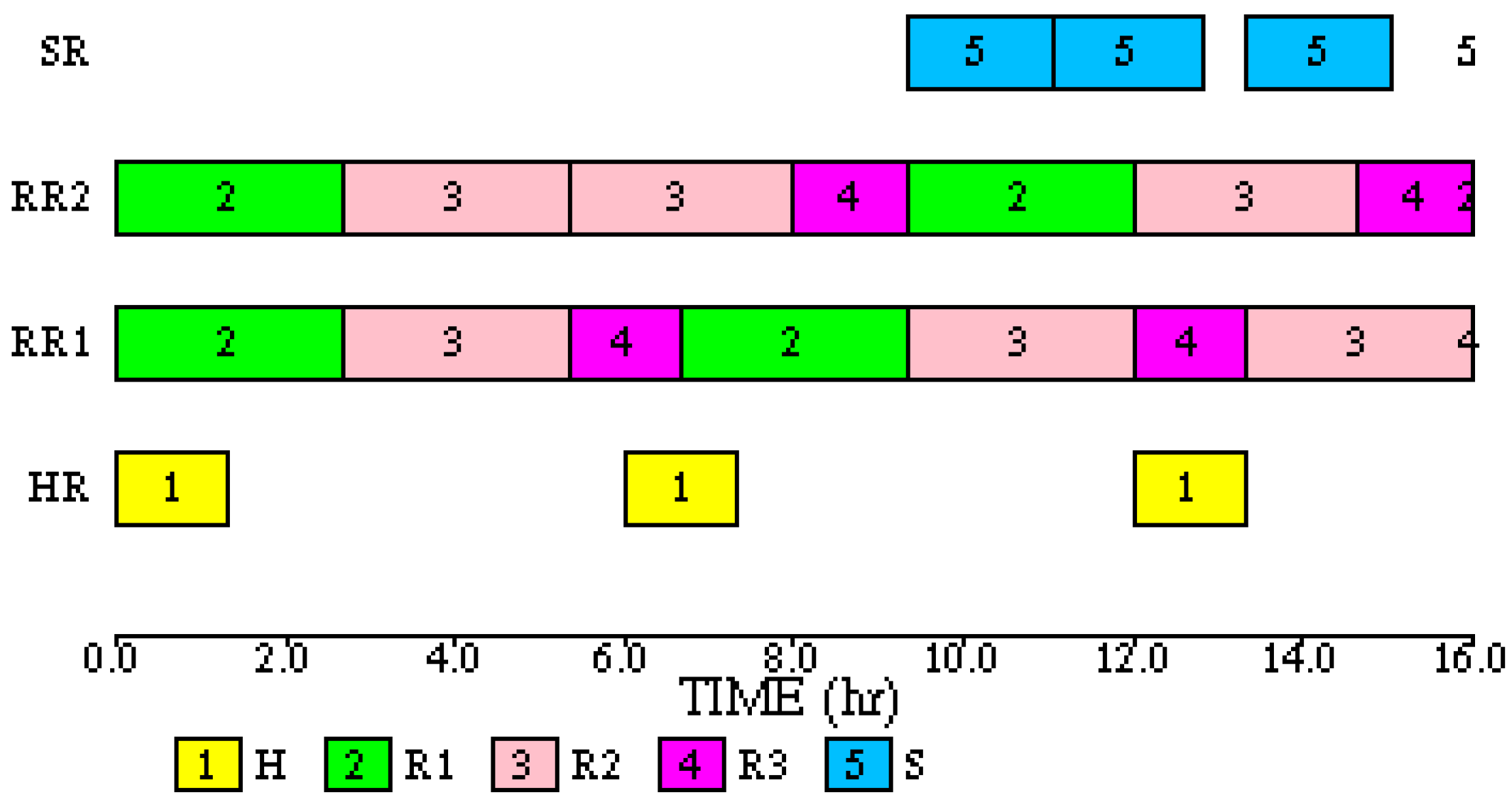
5.4. Example 4

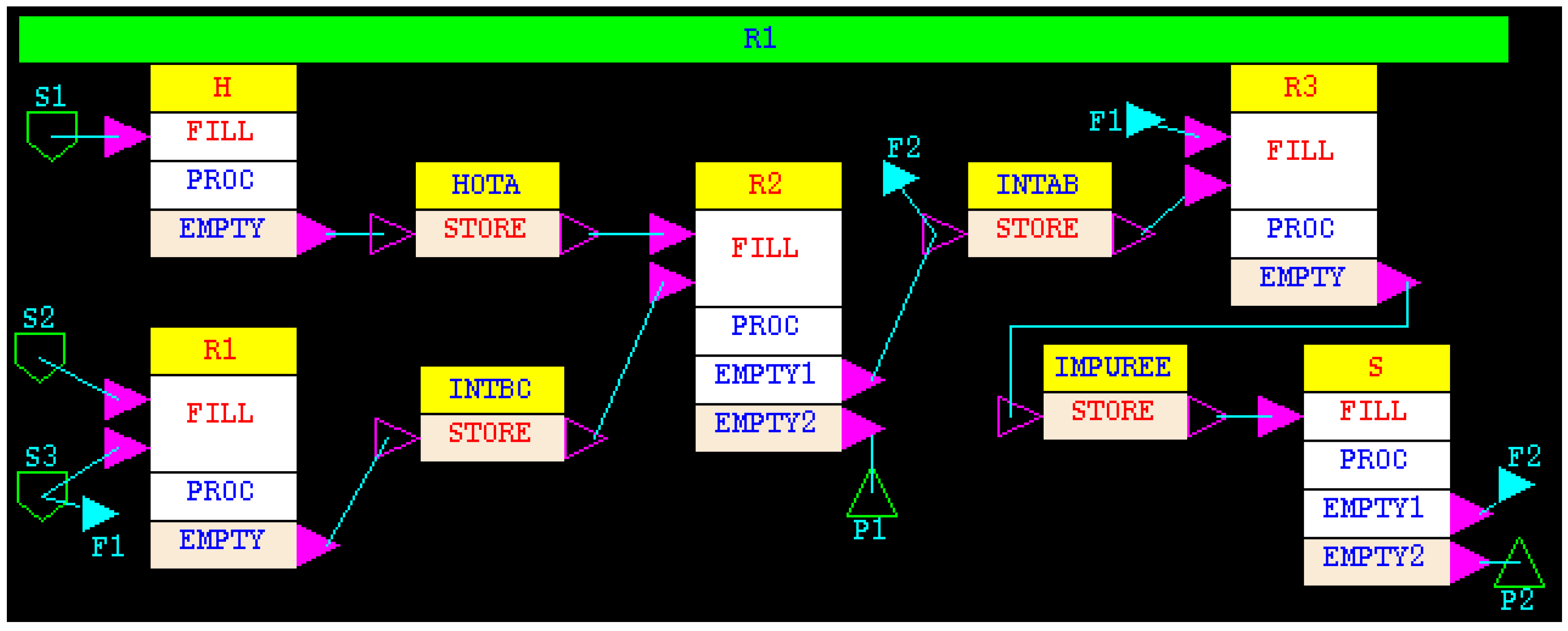
The recipe network for this example is shown in Figure 10. The key process parameters are given in

Table 4. Key process parameters for Example 4.

Task	Unit	α	β	M, kg	Input from (%)	Output to (%)
H	H	0.667	0.00667	100
R1	RR1	1.334	0.02664	50	S2: 50.0
	RR2	1.334	0.01665	80	S3: 50.0
R2	RR1	1.334	0.02664	50	HOTA: 40.0	INTAB: 60.0
	RR2	1.334	0.01665	80	INTBC: 60.0	P1: 40.0
R3	RR1	0.667	0.01332	50	S3: 20.0
	RR2	0.667	0.00833	80	INTAB: 80.0
S	SR	1.3342	0.00666	200		INTBC: 10.0 P2: 90.0

. Two reactors, RR1 and RR2, are suitable to perform tasks R1, R2, and R3. The reactors are of different size.

Two finished products are produced in this process, P1 and P2, which is lower quality P1. In addition to being multipurpose, there is recycling of the one of the streams from the last separation task S.

Processing directives were specified to initiate tasks R1, R2, R3, H and S. In addition, the priority of three was assigned for task R3, two for R2, and one for R1. A reactor was assigned to R2 only if enough material was available in INTBC and HOTA storage tanks. Similarly, a reactor was assigned to R3 only if enough material was available in INTAB storage tank. Thus, if material was available for R3, it was given preference over R2 and R1. If R3 could not be initiated and there was enough material for R2, then it was given preference over R1. Task R1 was initiated only when neither R2 nor R3 could be initiated. In the beginning when there is no intermediate material, both reactors are assigned to R1.

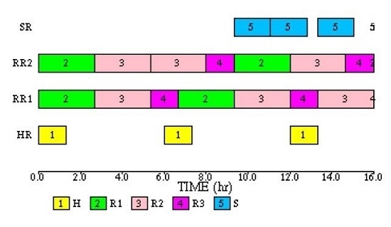
A time horizon of 16.0 h was used in this example. The Gantt chart is shown in Figure 11. The schedule generated by the simulation model is similar to the optimum schedule. As in the previous example, the optimizer was able to adjust batch sizes so as to fit complete batches in the given time horizon. The sequence of batches on individual reactors is different from the optimum schedule. The built-in rules do generate a sensible schedule within a fraction of the computing time. The total amounts produced are: 156.0 kg P1 and 162.0 kg P2. For the optimum solution the amounts produced are: 147.4 kg P1 and 225.9 kg P2. Again, the difference is due to the fact that the optimizer is able to do fractional batches to fit in the available time. In the simulation, at the end there is 60 kg in the separator which could make up the difference for P2.

The simulation run took 0.049 s (user + sys values from the Linux time command). All MILP formulations required more than 10,000 CPU s. Using the appropriate logic to assign equipment along with assigning priorities to resolve competition was sufficient to schedule this process.

The Gantt chart shows that there is no slack time on both RR1 and RR2. Therefore, it would not be possible to produce any more material.

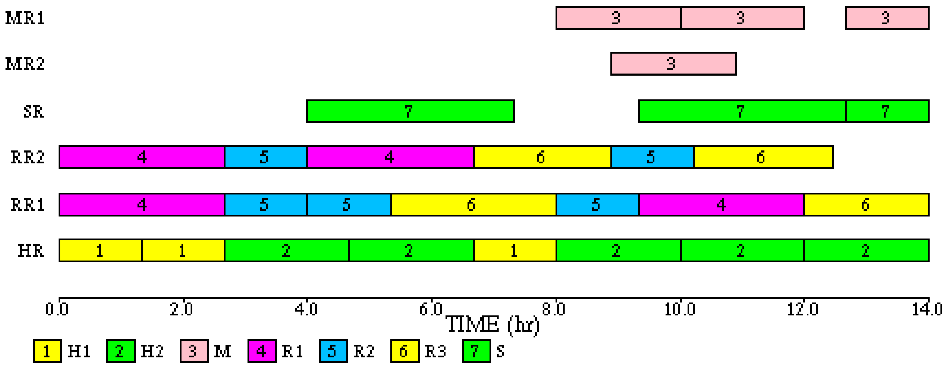
5.5. Example 5

This process is a variation of the recipe in Example 4. The recipe network for this example is shown in Figure 12. The key process parameters are given in

Table 5. Key process parameters for Example 5.

Task	Unit	α	β	M, kg	Input from (%)	Output to (%)	Throughput kg/h
H1	HR	0.667	0.00667	100			75.0
H2	HR	1.0	0.01	100	INT4: 25.0 S8: 75.0		50.0
R1	RR1 RR2	1.334 1.334	0.0133 0.00889	100 150			37.5 56.2
R2	RR1 RR2	0.667 0.667	0.00667 0.00445	100 150	INT1: 50.0 INT2: 50.0		75.0 112.4
R3	RR1 RR2	1.333 1.333	0.01333 0.00889	100 150		INT7: 60.0 P2: 40.0	37.5 56.2
S	SR	2.000	0.00667	300		INT4: 40.0 INT5: 50.0 INT2: 10.0	75.0
M	MR1 MR2	1.333 1.333	0.00667 0.00667	200 200	INT7: 40.0 INT5: 40.0 S11: 20.0		75.0

. The two reactors, RR1 and RR2, are suitable to perform tasks R1, R2, and R3. In addition, tasks H1 and H2 use the same unit, namely HR.

Preliminary stage throughput calculations were performed before developing the equipment assignment strategy. The maximum average throughputs for each unit for each task were calculated using the process parameters. The throughputs are given in Table 5. From the material balance, for every 1.0 kg output from R1, at least 2.0 kg output from R2 is produced, and at least 2.4 kg output from R3 is produced. The average maximum throughput of task R2 is twice that of R1. Therefore, tasks R1 and R2 are balanced. However, the average maximum throughputs of R1 and R3 are the same. Furthermore, one batch of H2 is required to make one batch of R3. The throughput of H2 is approximately half of the total throughput of RR1 and RR2 for task R3. Therefore, H2 is the bottleneck of the process. As a result, in addition to assigning high priority to initiate R3, more refined logic was added, namely that as long as there is more than a certain quantity of material in INT3, a batch of R2 was not initiated, and as long as there is more than a certain amount of material in INT2, a batch of R1 was not initiated. The refined logic was incorporated into the simulator as an external module. Similarly, since H1 and H2 compete for HR, the priority of H2 was set higher than that of H1.

At the beginning of the simulation, storage tanks S6 and S7 were initialized to contain 50.0 kg of INT4 and INT5, respectively, to match the condition specified in Susarla et al. [17]. Additionally, the batch size of 200.0 kg was used for task S. The Gantt chart for the simulation is shown in Figure 13. Initially, batches of R1 and R2 are made on the reactors RR1 and RR2. R3 can be initiated only after a batch of S and H2 is made.

For the specified time horizon of 14.0 h, 300.0 kg P1, and 120.0 kg P2 is produced, compared to 225.0 kg P1 and 160.0 kg P2.

The solution presented in Susarla et al. [17] has reactor batch sizes of 18.25 kg and 25.0 kg, which are one fifth of the size of the reactors, just so that some material can be produced in the available time. The simulation model produces different amounts of finished products, but the batch sizes are more realistic. As such, the process is not well balanced. Therefore an ‘optimum schedule’ may not have much practical significance.

The simulation run took 0.037 s (user + sys values from the Linux time command). All MILP formulations required more than 5000 CPU s. A more refined logic to assign equipment which was programmed as external module, along with assigning priorities to resolve competition was sufficient to schedule this process.

The Gantt chart shows that there is no slack time on HR. Therefore, it would not be possible to produce any more material.

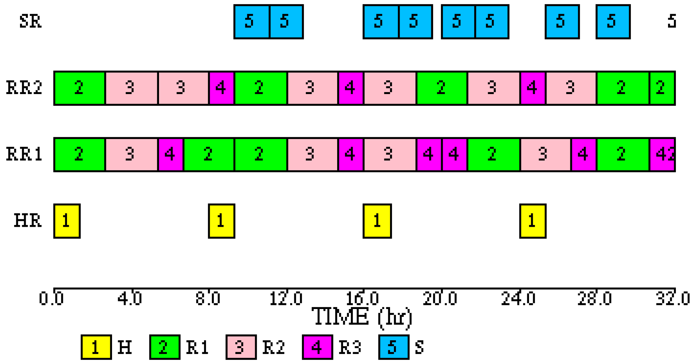
6. Advantages of Simulation

The number of variables in MILP formulations to solve scheduling problems increases exponentially as the time horizon increases. Consequently, the time required to solve the problems also increases exponentially. On the other hand, to simulate a process for longer time only one parameter, simulation end time, needs to change. The underlying model stays the same. As a consequence the computation time is typically linear with time horizon. Additionally, the quality of the schedule generated is not affected by the change in simulation time.

To demonstrate the linear dependency of computation time on simulation time, the process described in Example 4 was simulated for 32.0 h (double the original time of 16.0 h). The Gantt chart for this simulation run is shown in Figure 14.

The simulation run took 0.049 s (user + sys values from the Linux time command) which is, in fact, the same as the 16.0 h run. There is no MILP solution for this case.

The Gantt chart shows that there is no slack time on both RR1 and RR2. Therefore, it would not be possible to produce any more material.

7. Conclusions

In this paper we describe the enhanced capabilities to make better equipment assignment decisions which are available in the BATCHES simulator to facilitate its use in solving scheduling problems. To illustrate these capabilities, the simulator was used to schedule five batch processes for which various MILP formulations have been reported in the literature. In all cases the simulator generated very high quality solutions within a fraction of the time required for solving MILP formulations. Some solutions matched exactly the optimum solutions reported, while for some the results were different, but comparable. In certain cases, only a qualitative comparison could be made because of the inability of the simulator to make fractional batches. Even in those special cases, the assignment decisions made by the simulator were logical and verifiable. The recipe models of the processes studied in the test problems were not very complicated, most likely modified to keep the MILP formulations within manageable size. However, in general, the underlying recipes could be quite complex and can be handled easily by a simulation model with little or no impact on computation time. Once the modeling decisions are verified, the simulator can easily accommodate complexities such as parameter uncertainties, non-zero transfer times, sequence dependent cleaning, shared resources, and so on. The largest advantage of simulation is in tackling larger time horizons because the computation time is linear with time horizon. For MILP formulations, the number of variables increases exponentially with time horizon, often resulting in failure to find even a feasible solution. Simulation with more intelligence to make equipment assignment decisions can be a very effective tool in solving scheduling problems.