Model Predictive Control of the Exit Part Temperature for an Austenitization Furnace

Abstract

Quench hardening is the process of strengthening and hardening ferrous metals and alloys by heating the material to a specific temperature to form austenite (austenitization), followed by rapid cooling (quenching) in water, brine or oil to introduce a hardened phase called martensite. The material is then often tempered to increase toughness, as it may decrease from the quench hardening process. The austenitization process is highly energy-intensive and many of the industrial austenitization furnaces were built and equipped prior to the advent of advanced control strategies and thus use large, sub-optimal amounts of energy. The model computes the energy usage of the furnace and the part temperature profile as a function of time and position within the furnace under temperature feedback control. In this paper, the aforementioned model is used to simulate the furnace for a batch of forty parts under heuristic temperature set points suggested by the operators of the plant. A model predictive control (MPC) system is then developed and deployed to control the the part temperature at the furnace exit thereby preventing the parts from overheating. An energy efficiency gain of $5.3\%$ was obtained under model predictive control compared to operation under heuristic temperature set points tracked by a regulatory control layer.

1. Introduction

Countries around the world are aiming for economic growth that is inclusive, smart and sustainable. Research and innovation are key drivers to realize this transition [1,2,3,4,5,6]. Studies on power technologies and technological innovation as a means to achieve a more efficient energy-intensive industry, with reduced CO${}_2$ emissions are reported in the literature [7,8,9,10,11,12]. The iron and steel industry is not only energy-intensive but also one of the largest CO${}_2$ emitters [4,13,14]. The United States has the third largest national iron and steel sector in the world with annual crude steel production of $80.5$ million metric tonnes (Mt) in 2010 [15]. The iron and steel industry is the fourth largest industrial user of energy in the US with yearly demands of 2 quadrillion BTU (quads), which is roughly $2\%$ of the overall domestic energy consumption [16,17,18]. For an individual steel processing plant, reheating and heat treating furnaces account for $65\%$ to $80\%$ of the overall energy use [19,20]. The energy demand is intensified due to inherent furnace inefficiencies ($20\%$–$60\%$) and ineffective control strategies [20]. Therefore, any improvement in energy efficiency of steel processing furnaces through optimization, restructuring of processes and applying advanced control strategies will have a direct impact on overall energy consumption and related CO${}_2$ emissions.

Model predictive control (MPC), originally developed to meet specialized control needs of oil refineries and power plants, has now found applications in food processing, pharmaceutical, polymer, automotive, metallurgical, chemical and aerospace industries [21,22,23]. The success of MPC can be attributed, as summarized by Qin et al. [23], to its ability to solve complex multiple-input, multiple-output (MIMO) control problems

• without violating input, output and process constraints,
• accounting for disturbances,
• by preventing excess movement of input variables, and
• by controlling as many variables as possible in case of faulty or unavailable sensors or actuators.

In this work, we describe the development and implementation of an MPC system for controlling the temperatures of the parts exiting an industrial austenitization furnace using a model-based case study. The key to our approach is feedback control of the temperature of the metal parts (which can be measured in practice via a combination of non-contact temperature sensing and soft sensing/state observation). We show that, in this manner, the energy usage of the system is reduced considerably compared to the current regulatory control scheme (which is effectively open-loop with respect to product temperatures). To this end, we rely on the radiation-based nonlinear model of the furnace developed in Heng et al. [24] to develop a hierarchical, multi-rate control structure, whereby the setpoints of regulatory controllers are set by a multiple input, single output MPC that is computed at a much lower frequency than the regulatory control moves.

2. Process and System Description

Depending on the application, steel is forged into the desired shape and heat treated (e.g., annealed, quenched, and tempered) to improve its mechanical properties such as strength, hardness, toughness and ductility [25,26,27,28]. Among the heat treating processes, quench hardening is commonly employed to strengthen and harden the workpieces. Quench hardening consists of first heating finished or semi-finished parts made of iron or iron-based alloys to a high temperature, in an inert atmosphere, such that there is a phase transition from the magnetic, body-centered cubic (BCC) structure to a non-magnetic, face-centered cubic (FCC) structure called austenite (austenitization), followed by rapid quenching in water, brine or oil to introduce a hardened phase having a body-centered tetragonal (BCT) crystal structure called martensite [28,29,30,31]. This process is usually followed by tempering in order to decrease brittleness (increase toughness) that may have increased during quench hardening [28,32,33]. In this process of strengthening, austenitization is the energy-intensive step, where the workpieces have to be heated from typically 300 K to 1100 K in a furnace fired indirectly (to avoid oxidation) by radiant tube burners that require a large amount of fuel [27]. The part temperatures, especially the core, cannot typically be sensed and measured while the part is being processed inside the furnace. Nevertheless, the temperatures of the parts after exiting the furnace can be measured by non-contact ultrasonic measurements [34,35,36]. In practice, the operators tend to overheat the parts such that a minimum temperature threshold is exceeded, thereby causing excess fuel consumption. Another reason for overheating is that even if a single portion of the part does not transform to austenite completely during heat treatment, that portion will be very soft in the quenched product resulting in the entire part not meeting the quality standards. Therefore, the monetary gain in energy minimization while heating will be counter-balanced by the loss due to scrapping of defective parts. The temperature sensing limitations, combined with high energy usage, make austenitization furnaces primary targets for advanced model-based analysis and control.

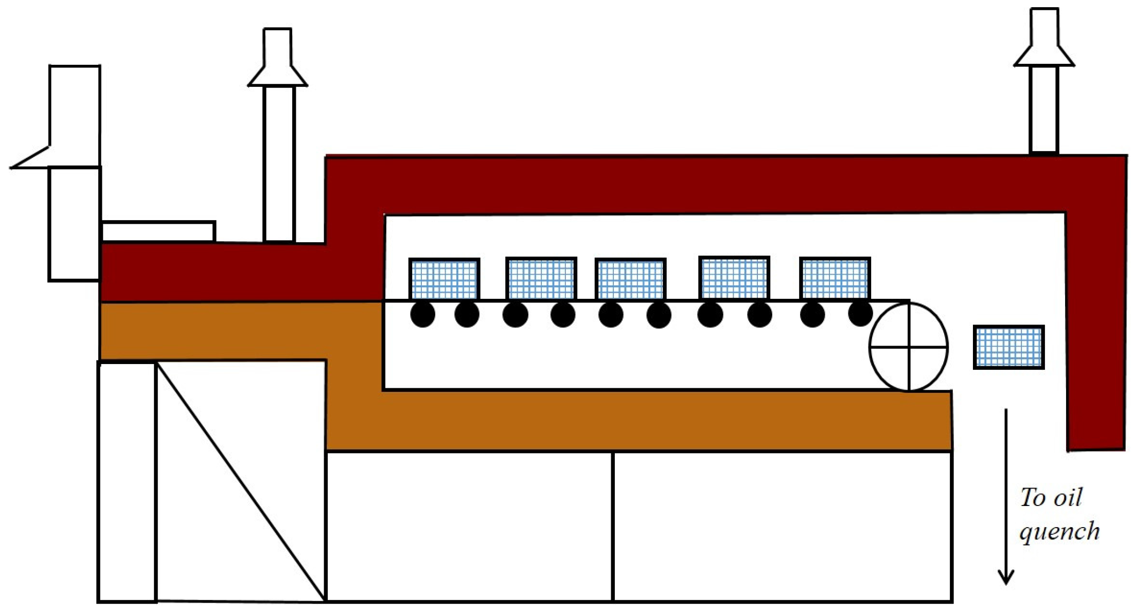
The austenitization furnace considered in this work is operated in a continuous manner under temperature feedback control (see Figure 1). Metal parts are loaded on to trays placed on a conveyor belt, which transports the parts through the furnace that is heated by combustion of natural gas in radiant tube burners on the ceiling and floor. After exiting the furnace, the parts are placed into an oil quench bath to induce the crystal structure change. Nitrogen is used as the inert blanket gas to prevent surface oxidation and flows counter current to the direction of motion of the conveyor belt. The furnace operates at temperatures in excess of 1000 K and the residence time of the parts is in the order of hours. Due to sensing limitations (equipment for the aforementioned ultrasonic measurements is not available in the plant), the part temperatures are currently indirectly controlled by controlling the furnace temperature—a scheme that is effectively open-loop with respect to part temperature control. The temperature set points of the local feedback controllers are set heuristically by process operators.

A two-dimensional (2D) radiation-based semi-empirical model of the furnace under consideration was developed in Heng et al. [24]. The model neglects the interactions between parts, which are cylindrical with ogive top shapes, and are loaded on a tray. The ensemble of a tray and its contents is modeled as a rectangular structure with equivalent metal mass and referred as to a “part.” The mass of the conveyor belt is much smaller than that of the part. Hence, the conveyor belt is excluded from the model. Nevertheless, the movement of the parts inside the furnace is captured. There is only surface-to-surface radiation interaction and no gas-to-surface radiation interaction since nitrogen is a diatomic molecule [38]. The gas-to-surface heat transfer is assumed to occur only through convection, and surface-to-surface heat transfer is assumed to occur only though radiation. 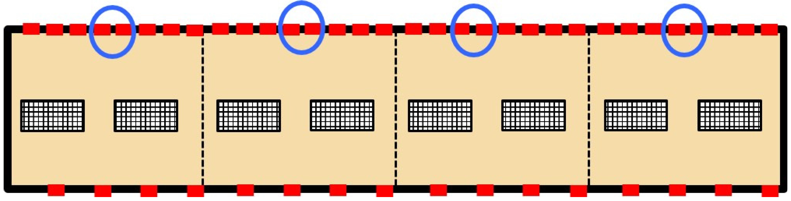The furnace is discretized into a series of control volumes to calculate a discretized gas temperature profile within the furnace. For temperature control purposes, adjacent burners are grouped together and the fuel flow rates are adjusted simultaneously for each group. The furnace is divided into four such groups (four control valves) of twelve burners each referred to as temperature control zones. The middle insulating surface of the ceiling of each zone is assumed to host the temperature sensor used for control (see Figure 2). The inputs to the model are the dimensions of the steel parts and its physical properties, the mass flow rate of fuel to the burners, feedback control zone temperature set points, flow rate of nitrogen, and the temperature of the surrounding air. The model evaluates the energy consumption of the furnace and the temperature distribution within the parts as a function of time and part position within the furnace.

We now follow the discussion of Heng et al. [24] to present an overview of the furnace model. In this model, the geometric elements of the furnace are discretized into a set of surfaces, namely, burner, insulation and load/part (see Figure 2). The overall energy balance of a surface i can be written as:

$$Q_{net,i}=Q_{radiation,i}+Q_{convection,i}i=1,\dots ,N_s,$$

(1)

where $N_s$ is the total number of surfaces (that change as the parts are loaded on to and unloaded from the furnace). $Q_{net,i}$, $Q_{radiation,i}$ and $Q_{convection,i}$ are the total heat transfer, radiative heat transfer and convective heat transfer, respectively, to surface i. The following two relationships are used for radiation heat transfer term [38]:

$$Q_{radiation,i}=\frac{\sigma {T_i}^4-J_i}{\frac{1-{ϵ}_i}{{ϵ}_i{A}_i}},$$

(2)

$$Q_{radiation,i}=\sum _{j=1}^{N_s}\frac{J_i-J_j}{{\left(A_i{F}_{i,j}\right)}^{-1}},$$

(3)

where $T_i$ is the temperature of surface i, $J_i$ is the radiosity of surface i, $A_i$ is the area of surface i, $F_{i,j}$ is the view factor from surface j to surface i, σ is the Stefan–Boltzmann constant and ${ϵ}_i$ is the emissivity of surface i. Radiosity $J_i$ is defined as the net amount of heat leaving surface i via radiation and view factor $F_{i,j}$ is defined as the proportion of the heat due to radiation that leaves surface j and strikes surface i.

For burner surfaces, Equation (2) is substituted into Equation (1) to obtain:

$$Q_{net,i}-h_{furn}{A}_i\left(T_i-T_w^{\infty }\right)=\frac{\sigma {T_i}^4-J_i}{\frac{1-{ϵ}_i}{{ϵ}_i{A}_i}},$$

(4)

where $h_{furn}$ is the heat transfer coefficient of the furnace and $T_w^{\infty }$ is the temperature of gas in control volume w. The term, $h_{furn}{A}_i\left(T_i-T_w^{\infty }\right)$, captures the convective heat transfer between a burner surface i and the gas in control volume w. The heat transfer coefficient of furnace $h_{furn}$ is calculated from a Nusselt number correlation for forced convection in turbulent pipe flow [38]. For a burner surface, the heat duty $Q_{net,i}$ and surface temperature $T_i$ are input variables determined by solving a system of nonlinear differential algebraic equations (DAE) that capture the dynamics of the burner system.

For insulation surfaces, Equation (3) is substituted into Equation (1) to obtain:

$$Q_{net,i}-h_{furn}{A}_i\left(T_i-T_w^{\infty }\right)=\sum _{j=1}^{N_s}\frac{J_i-J_j}{{\left(A_i{F}_{i,j}\right)}^{-1}}.$$

(5)

Note that, for the insulation surfaces, $Q_{net,i}$ and $T_i$ are output variables. The insulating wall is modeled as a solid material with uniform thickness. $Q_{net,i}$ is used as a Neumann type boundary condition at the inner surface to solve the one-dimensional unsteady state heat equation (parabolic partial differential equation) by an implicit Euler finite difference scheme:

$$Q_{net,i}=-k_{ins}{A}_i\frac{d{T}_i}{d{\overrightarrow{x}}_i},$$

(6)

where $T_i$ is the temperature of the inner surface of insulation i, $A_i$ is the area of insulation surface i, $k_{ins}$ is the thermal conductivity of insulating material (brick) and ${\overrightarrow{x}}_i$ is the inward unit normal vector to the insulating surface i. The other boundary condition is the balance between heat conduction through the wall to the outer surface and convective heat transfer between the outer surface and the ambient air, expressed as:

$$k_{ins}{A}_i\frac{d{T}_{ins,out,i}}{d{\overrightarrow{x}}_i}=-h_{air}{A}_i(T_{ins,out,i}-T_{air}),$$

(7)

where $T_{ins,out,i}$ is the temperature of the outer surface of insulation i and $h_{air}$ and $T_{air}$ are the convective heat transfer coefficient and the temperature, respectively, of the ambient air. The view factor matrix, $F_{i,j}$, is calculated using Hottel’s crossed string method [39].

Part surfaces are treated similarly to insulating surfaces, except that the furnace heat transfer coefficient $h_{furn}$ is replaced by the part heat transfer coefficient $h_{part}$:

$$Q_{net,i}-h_{part}{A}_i\left(T_i-T_w^{\infty }\right)=\sum _{j=1}^{N_s}\frac{J_i-J_j}{{\left(A_i{F}_{i,j}\right)}^{-1}}.$$

(8)

The part heat transfer coefficient $h_{part}$ is obtained from a Nusselt number correlation for external flow over a square cylinder [38]. A part is assumed to be a uniform solid. The two-dimensional unsteady state heat equation is solved by a second-order accurate Crank–Nicolson finite difference method to obtain the spatial temperature distribution of a part. The net heat flux, $Q_{net,i}$, of the four surfaces encompassing a part are used to define the boundary conditions:

$$Q_{net,i}=-k_{part}{A}_i\frac{d{T}_i}{d{\overrightarrow{n}}_i},$$

(9)

where $k_{part}$ is the thermal conductivity of part, $T_i$ and $A_i$ are the temperature and area of part surface i and ${\overrightarrow{n}}_i$ is the inward unit normal vector to part surface i.

At each time step, the model evaluates the energy usage of the furnace by solving Equations (4), (5) and (8) for the heat duties and the temperatures of insulation and part surfaces using a dual iterative numerical scheme explained in Heng et al. [24]. The computed heat duties are then used to define the boundary conditions to determine the part temperature distribution for all the parts processed in the furnace. Additionally, a linear control strategy is adopted, wherein a proportional-integral (PI) controller controls the temperature of each zone to a given set point by appropriately adjusting the mass flow rate of fuel to the burners of the respective zone. The temperature set points of the PI controllers directly affect the temperature distribution of the parts in the furnace and thus the energy consumption of the system.

3. Model Predictive Control Development

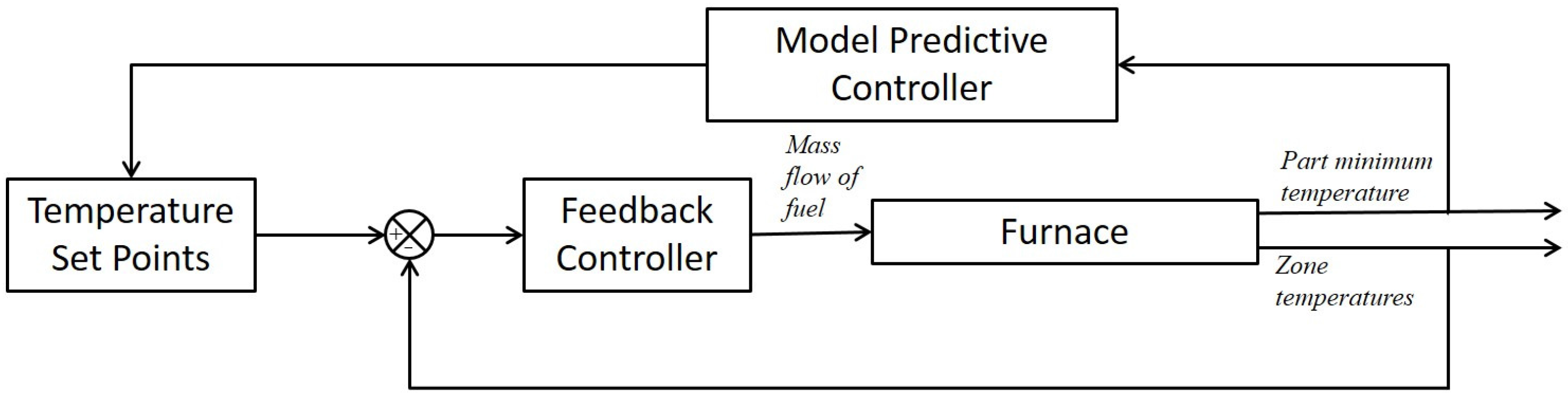
In our system, model predictive control is implemented as a two-layer hierarchical structure. The inner layer is the aforementioned regulatory control that manipulates the mass flow rate of fuel to control the zone temperatures. This multiple-input, single output system is then considered in the outer layer, whereby the model predictive controller adjusts the temperature set points of the regulatory layer to control the minimum temperatures of parts at exit. Note that the time interval for control action of model predictive control is larger than that of regulatory control, as will be explained below. The block diagram of the implementation of model predictive control in the heat treating furnace is shown in Figure 3.

Let $T_{sp,\psi }\left(k\right),\forall \psi \in [1,4]$ be the temperature set point of zone ψ at sampling instant k, and $T_{min}\left(k\right)$ be the part minimum temperature at exit of the furnace. Let $T_{sp,ss,\psi },\forall \psi \in [1,4]$ be the steady-state temperature set point of zone ψ and $T_{min,ss}$ be the steady-state part minimum temperature. Additionally, let $y\left(k\right)$ be the deviation variable of part minimum temperature at time instant k, defined as: $y\left(k\right)\triangleq T_{min}\left(k\right)-T_{min,ss}$ and $u_{\psi }\left(k\right)$ be the deviation variable of zone ψ temperature set point at k, defined as: $u_{\psi }\left(k\right)\triangleq T_{sp,\psi }\left(k\right)-T_{sp,ss,\psi },\forall \psi \in [1,4]$.

3.1. Construction of MPC Step-Response Model

The step-response model of a stable process with four inputs and one output can be written as:

$$\begin{array}{cc}\hfill y(k+1)=y\left(0\right)& +\sum _{i=1}^{N-1}{S}_{1,i}\Delta u_1(k-i+1)+S_{1,N}{u}_1(k-N+1)\hfill \\ & +\sum _{i=1}^{N-1}{S}_{2,i}\Delta u_2(k-i+1)+S_{2,N}{u}_2(k-N+1)\hfill \\ & +\sum _{i=1}^{N-1}{S}_{3,i}\Delta u_3(k-i+1)+S_{3,N}{u}_3(k-N+1)\hfill \\ & +\sum _{i=1}^{N-1}{S}_{4,i}\Delta u_4(k-i+1)+S_{4,N}{u}_4(k-N+1),\hfill \end{array}$$

(10)

where $y(k+1)$ is the output variable at the $k+1$ sampling instant, $y\left(0\right)$ is the initial value of the output variable, and $\Delta u_{\psi }(k-i+1)$ for $\psi \in [1,4]$ denotes the change in the input ψ from one sampling instant to the next: $\Delta u_{\psi }(k-i+1)=u_{\psi }(k-i+1)-u_{\psi }(k-i)$. Both u and y are deviation variables defined earlier in this paper. The model parameters are the N step-response coefficients, $S_{\psi ,i}$ to $S_{\psi ,N}$, for each input $\psi ,\forall \psi \in [1,4]$. Therefore, the total number of step-response coefficients are $4N$, where N is selected based on the process time constants.

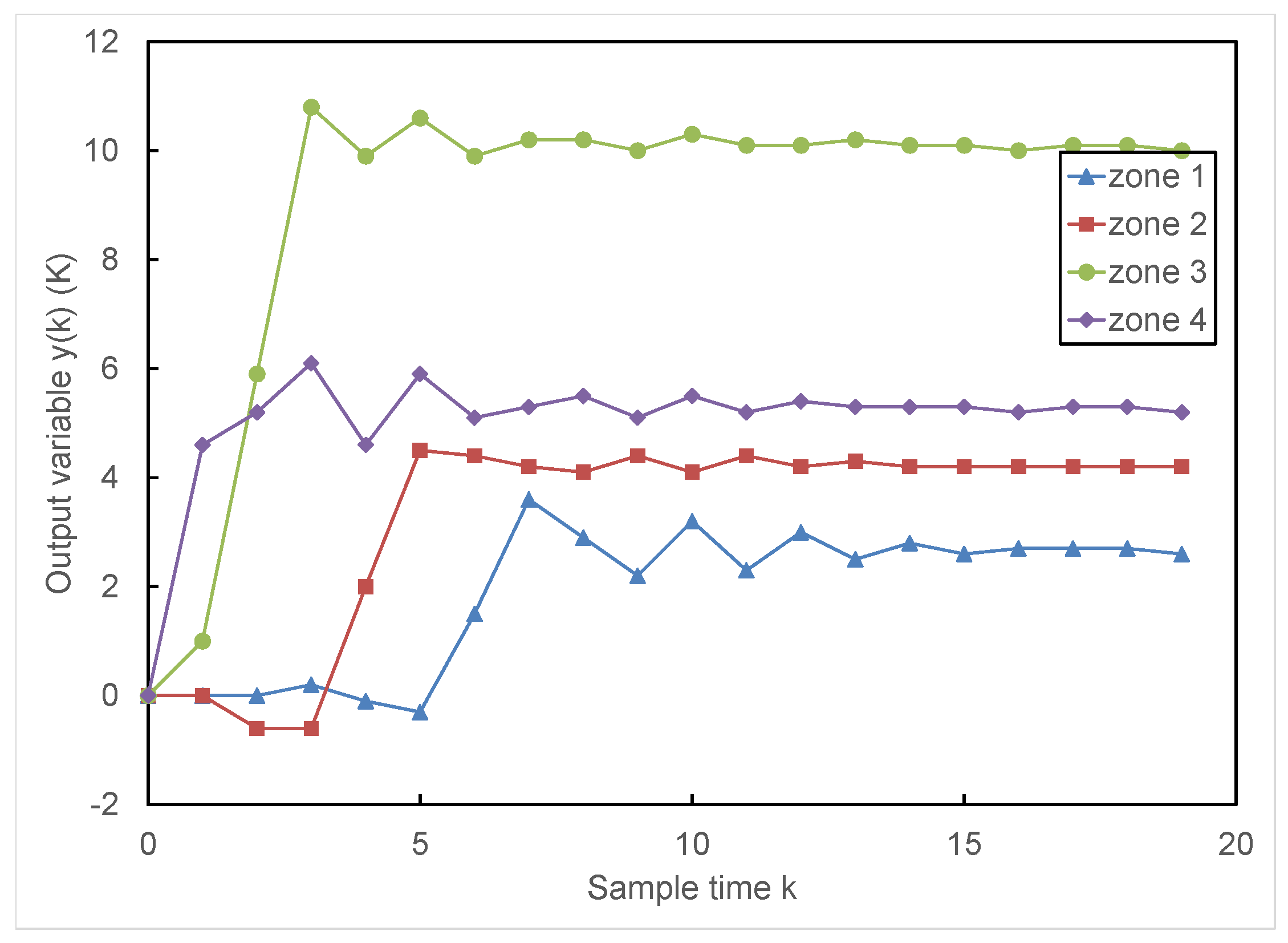
The response of the output variable $y\left(k\right)$ for a step input $\Delta T_{step}$ of 20 K in each zone temperature set point is shown in Figure 4. The furnace takes about 25 h to process a batch of 40 parts with part residence time being roughly 4 h. The time difference between the exit of successive parts is the control time step $\Delta t_{MPC}$, which is around 32 min. The design variable N, which is the number of step-response coefficients for each control input was taken as 19. The step-response coefficients can be calculated from the step-response data [40]. It can be inferred from Figure 4 that the zone 3 temperature set point has the dominant effect on the part exit temperature, and zone 1 has the least.

3.2. Optimization Formulation

Following the derivation of MPC from Seborg et al. [40], the vector of control actions $\Delta \mathit{U}\left(k\right)$ for next M sampling instants (the control horizon) is calculated at each sampling instant k by minimizing the objective function shown below, subject to the input, output and process constraints. The optimization problem formulation is:

$$\begin{array}{cccc}& \underset{\Delta \mathit{U}\left(k\right)}{\mathrm{minimize}}\hfill & & \mathit{J}=\widehat{\mathit{E}}{(k+1)}^T\mathit{Q}\widehat{\mathit{E}}(k+1)+\Delta \mathit{U}{\left(k\right)}^T\mathit{R}\Delta \mathit{U}\left(k\right)\hfill \\ & \mathrm{subject}\mathrm{to}\hfill & & u_{\psi }(k+j)\ge u_{min},\psi \in [1,4]\mathrm{and}j\in [0,k+M-1]\hfill \\ & & & u_{\psi }(k+j)\le u_{max},\psi \in [1,4]\mathrm{and}j\in [0,k+M-1]\hfill \\ & & & u_{\psi }(k+j)-u_{\psi +1}(k+j)\le u_{diff},\psi \in [1,3]\mathrm{and}j\in [0,k+M-1]\hfill \\ & & & SystemModel(\mathrm{Equation} \left(10\right)),\hfill \end{array}$$

(11)

where $\mathit{Q}$ and $\mathit{R}$ are the output and input weighting matrices, respectively, that allow the output and input variables to be weighted according to their relative importance. $\widehat{\mathit{E}}(k+1)$ is the predicted error vector of length P (prediction horizon) between the target and the model predictions (including bias correction) at $k+1$ sampling instant. $u_{min}$ and $u_{max}$ are the lower and upper bounds of the zone temperature set points $u_{\psi },\psi \in [1,4]$ respectively, and $u_{diff}$ is the minimum possible positive temperature difference between consecutive zones in the direction of part movement in order to prevent loss of heat from parts to the furnace while processing. Note that $u_{min}$, $u_{max}$ and $u_{diff}$ are deviation variables. Once $\Delta \mathit{U}\left(k\right)$ is computed, the furnace simulation proceeds for the control time interval $\Delta t_{MPC}$, during which the sample time is updated from k to $k+1$ and the entire procedure is repeated.

4. Furnace Simulation under Model Predictive Control

We simulate the furnace for a batch of forty parts using the same parameters and operating conditions as those in Heng et al. [24] under temperature feedback control. Additionally, instead of operating at a constant heuristic temperature set points suggested by the operators of the plant, the supervisory model predictive controller changes the zone temperature set points to control the part temperature at exit of the furnace (see Figure 3). The lower-layer temperature tracking controllers use the above trajectory as the control target. At the regulatory level, a linear control strategy is adopted wherein the fuel mass flow rate of a zone is manipulated to minimize the error between the measured value of the respective zone temperature and its set point determined by the MPC. All the burners in a zone are adjusted simultaneously, i.e., the furnace has only four control valves for regulatory control. In practice, a butterfly valve is used to manipulate the fuel flow rate. This valve does not close fully, i.e., the mass flow rate of fuel to the burners does not drop below a certain lower limit. In addition, when the valve is fully open, the upper bound of fuel flow rate is reached. Each control zone operates independently of other zones. However, adjustments to fuel flow rate of one zone will affect the temperatures of other zones due to long range radiation interactions. The furnace operating conditions and the parameters used in the simulation are listed in

Table 1. List of parameters used in the heat treating furnace simulation.

Furnace Details
Length of the furnace	16 m
Height of the furnace/length of the side walls	2 m
Length of each discretized furnace surface except the side walls	$0.25$ m
Total number of furnace surfaces	130
Length of a part	$1.25$ m
Ordinate of a part	$0.75$ m
Height of a part	$0.5$ m
Process Conditions
Number of parts processed	40
Inlet temperature of parts	300 K
Inlet temperature of blanket gas	400 K
Number of points in the x-direction for Crank–Nicolson method	6
Number of points in the y-direction for Crank–Nicolson method	6
Total time of furnace operation	25 h
Feedback control time interval	4 min
Model Predictive Control Details
Target minimum part temperature at exit	1088 K
Lower bound of temperature set points	900 K
Upper bound of temperature set points	1300 K
Temperature set point difference between subsequent zones	30 K
Model predictive control time interval	$32.5$ min

. The local control sampling time is 4 min for the 25 h furnace operation. The upper level model predictive controller functions at a much longer time interval, with a sampling time of $32.5$ min, correlated with the rate of input/output of parts to the furnace. Within this time period, there are about eight control moves for the inner level temperature tracking controllers to bring the zone temperatures closer to the trajectory determined by the MPC. The setpoint for the MPC controller is the part minimum temperature at exit of the furnace. Note that non-contact ultrasonic measurements can be used to measure the value of minimum part temperature at the exit of the furnace [34,35,36]. However, non-contact measurements of the part temperatures, while the part is being processed inside the furnace, would be inaccurate due to the interference of the ultrasonic signal with the furnace walls. We use a constant target value of 1088 K, a temperature that ensures complete transformation from pearlite (mixture of ferrite and cementite) to austenite for a steel with $0.85\%$ carbon content.

As a base case, we consider a simulation where only the regulatory control layer is employed, with the temperature set points, $T_{sp,ss,\psi }\forall \psi \in [1,4]$, taken to be same as the heuristic temperature set points of Heng et al. [24]: 1000 K, 1150 K, 1200 K, 1250 K for zones 1 to 4, respectively. Furnace operation under these set points results in an exit part minimum temperature at constant part input rate of 1126 K. This is the steady state value of the output variable $T_{min,ss}$.

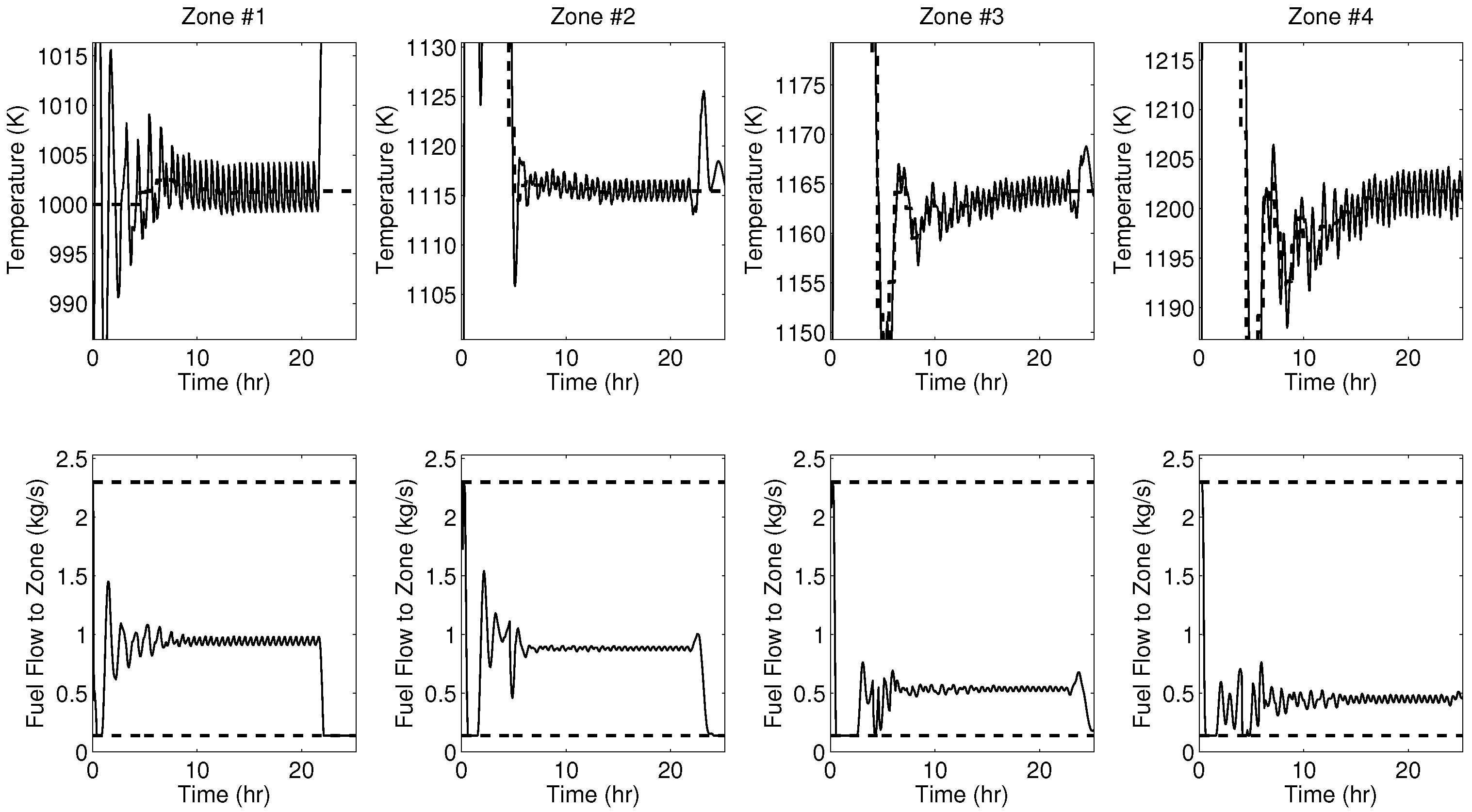
Then, we consider the furnace operation under the proposed MPC scheme. Figure 5 illustrates the variation of output and input variables with respect to time of furnace operation in this case. The model predictive controller is turned on only after about 4 h of furnace operation when the first part exits the furnace, at which point the furnace begins to operate in a regime characterized by constant rates of input and output of parts. Note that the furnace is not completely full during the last 4 h of operation as well. The plots in the top row of Figure 5 show the zone temperature setpoints (as set by the MPC) and the zone temperatures maintained by the regulatory control layer at these setpoints within minimal variations (in general within 5 K). The step-response plot in Figure 4 indicates that zone 3 and zone 4 temperature set points have dominant effects on exit part temperature. This aspect is also reflected in Figure 5, where it can be seen that the set point variations are higher in zones 3 and 4 to meet the target. It is also observed that the zone temperatures exhibit periodic oscillations around their set points. This effect can be attributed to the periodic entry of cold parts into the furnace in zone 1 and periodic removal of hot parts from the furnace in zone 4. The thermal gradient is the maximum when a cold part enters the furnace. Therefore, the part acts as a heat sink resulting in a rapid decrease in the temperature of zone 1. This disturbance is propagated to other zones of the furnace due to long range zone-to-zone radiation interactions. Moreover, additional harmonics in the temperature variations are caused by parts exiting the furnace. The plots in the bottom row of Figure 5 show the corresponding changes in the manipulated variable, i.e., the mass flow rate of fuel to the burners. The dashed lines in these plots represent the lower and upper bounds of the fuel flow rate.

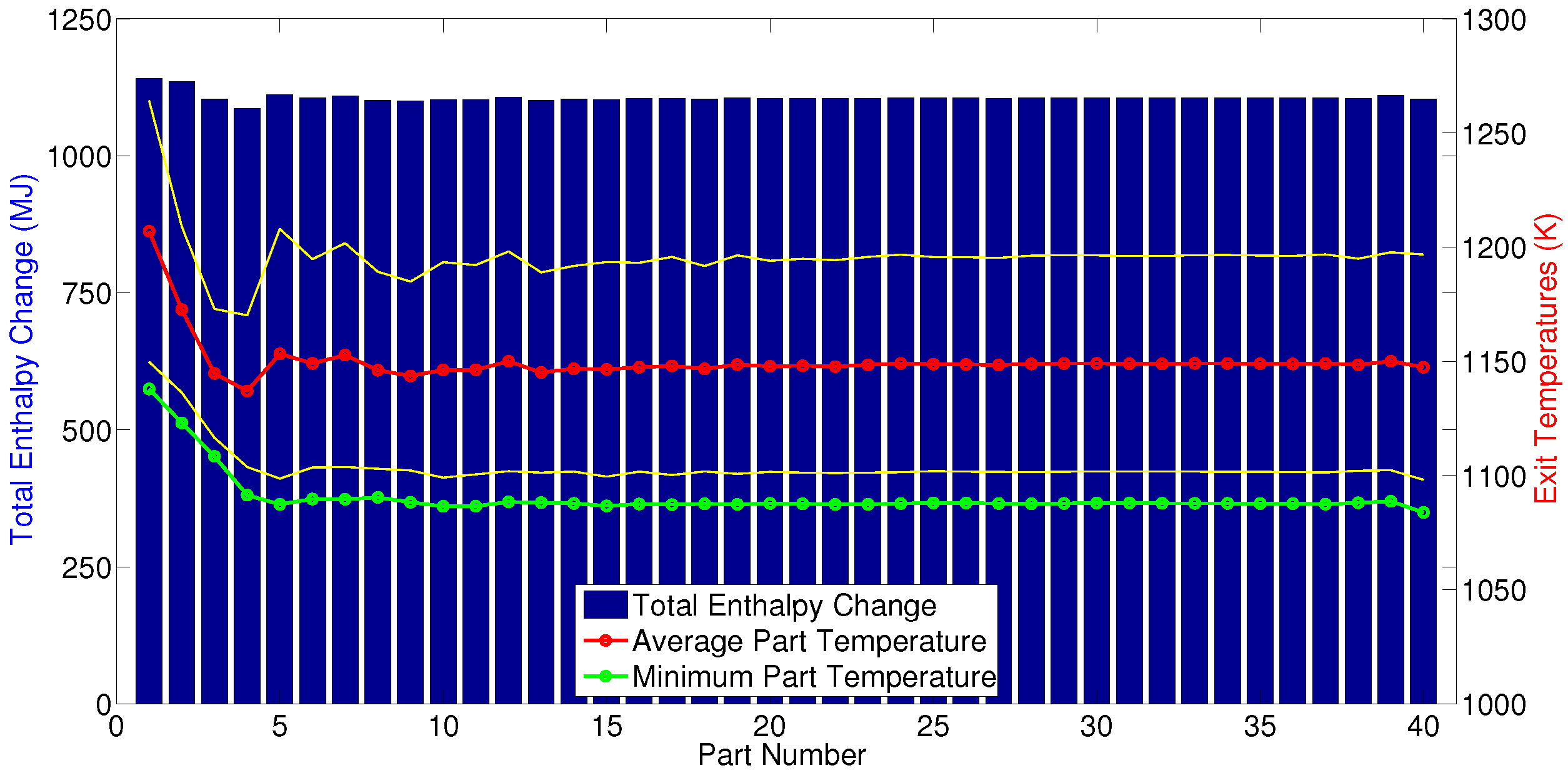
Figure 6 shows the exit conditions of all the processed parts exiting the furnace sequentially. The quantities plotted are the total change in part enthalpy and its temperature distribution details. The red curve represents the average of part temperature distribution of all parts at exit, yellow curves are its standard deviation and the green curve represents the minimum of the temperature of all the parts at exit, which is the target for the model predictive controller. The temperature set point changes made by the model predictive controller drive the part minimum temperature from around 1125 K for the first part to the target value of 1088 K. The two-tiered control strategy keeps the exit conditions relatively stationary once part minimum temperature reaches its target.

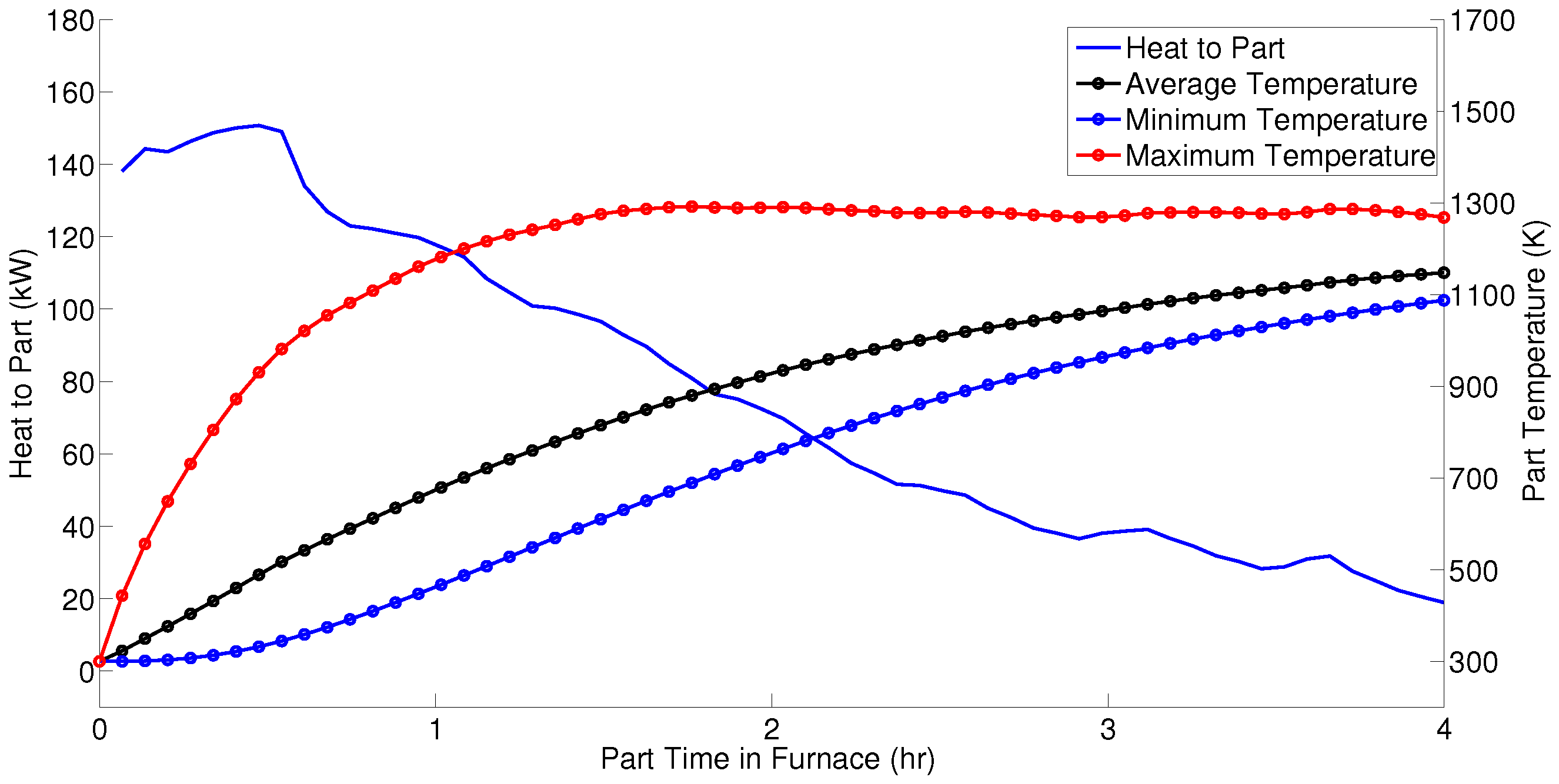
Finally, we plot the heat input to the 20th part and the parameters of the part temperature distribution with respect to processing time in Figure 7. Note that the residence time of a part is roughly 4 h. Therefore, the time spent within the furnace also corresponds to the zone in which the part is getting heated. As expected, the amount of heat transferred to a part decreases with time since, as the part becomes hotter, the temperature difference between the part and the burners becomes smaller. The maximum temperature of a part is at its boundary/exterior. Intuitively, the minimum temperature occurs at the interior (which is heated only via conduction), and hence the corresponding temperature gradually raises to its target value as the parts exit the furnace.

5. Energy Efficiency Comparison

In

Table 2. Total energy input to the furnace and part temperature distribution at the exit of the furnace under heuristic operation mode of Heng et al. [24] and two-level hierarchical control. We also show the energy distribution of the heat input to process a batch of 40 parts.

Heat Sources and Sinks	Heuristic Set Points	Model Predictive Control
Total Energy Input per Part (GJ)	$3.76$ GJ	$3.56$ GJ
Part Minimum Temperature (K)	1126 K	1088 K
Temperature Standard Deviation (K)	52 K	46 K
Energy to Parts (%)	$54.2\%$	$54.3\%$
Energy Lost with the Exhaust (%)	$42.7\%$	$42.5\%$
Energy to Flowing Nitrogen (%)	$0.5\%$	$0.5\%$
Energy Through Insulation (%)	$2.6\%$	$2.7\%$

, we compare the furnace operation under regulatory control with heuristic zone temperature set points reported in Heng et al. [24] and under model predictive control. In heuristic operation mode, the minimum temperature of parts at exit, 1126 K, is higher than the desired value of 1088 K. This overheating of parts results in the furnace consuming additional fuel. Furthermore, overheating of parts results in austenite grain size growth, which adversely affects the toughness of the quenched product. However, under the two layer hierarchical control operating mode, the part exit temperature is maintained at its desired value of 1088 K. The energy metric we compare is the total energy input to the furnace per part processed. We see that the furnace operation under model predictive control requires $5.3\%$ less energy than that under a heuristic operation scenario. The energy efficiency gain is mainly due to the lowered fuel use. Moreover, additional gains can be a consequence of different nonlinear surface-to-surface radiation interactions due to changing zone temperature set points. The standard deviation of part temperatures is similar in both of these operation modes. This means that the model predictive controller has maintained the minimum temperature of part at exit at its desired value without compromising the uniformity in heating. The distribution of energy input to the furnace to parts, exhaust, nitrogen and insulation are comparable for both of these operation modes.

6. Conclusions

In this work, a two-dimensional radiation-based model of the furnace developed in Heng et al. [24] is used to simulate an industrial radiant tube roller hearth heat treating furnace for a batch of 40 parts. The model computes the energy consumption of the furnace by solving energy conservation equations and evaluates the temperature distribution of parts as a function of time and position within the furnace using the Crank–Nicolson finite difference method. For control purposes, the furnace is divided into four zones. The zone temperature is controlled by a proportional-integral controller that simultaneously manipulates the fuel to all the burners of the respective zones.

Model predictive control is then implemented as a supervisory control to limit the part temperature at exit by varying the zone temperature set points of the regulatoryl temperature tracking controller. We first develop a step-response model to predict the future evolution of the output variables. The time interval of the model predictive control is longer than that of the regulatory control. A comparison in terms of energy consumption is made between the furnace operation under the two-level hierarchical control and under constant heuristic temperature set points reported in Heng et al. [24]. We obtain an energy efficiency gain of $5.3\%$ under model predictive control by preventing the parts from overheating.