Targeted Stimulation Using Differences in Activation Probability across the Strength–Duration Space

Abstract

Electrical stimulation is ubiquitous as a method for activating neuronal tissue, but there is still significant room for advancement in the ability of these electrical devices to implement smart stimulus waveform design to more selectively target populations of neurons. The capability of a device to encode more complicated and precise messages to a neuronal network greatly increases if the stimulus input space is broadened to include variable shaped waveforms and multiple stimulating electrodes. The relationship between a stimulating electrode and the activated population is unknown; a priori. For that reason, the population of excitable neurons must be characterized in real-time and for every combination of stimulating electrodes and neuronal populations. Our automated experimental system allows investigation into the stimulus-evoked neuronal response to a current pulse using dissociated neuronal cultures grown atop microelectrode arrays (MEAs). The studies presented here demonstrate that differential activation is achievable between two neurons using either multiple stimulating electrodes or variable waveform shapes. By changing the aspect ratio of a rectangular current pulse; the stimulus activated neurons in the strength–duration (SD) waveform space with differing probabilities. Additionally, in the case when two neuronal activation curves intersect each other in the SD space; one neuron can be selectively activated with short-pulse-width; high-current stimuli while the other can be selectively activated with long-pulse-width; low-current stimuli. Exploring the capabilities and limitations of electrical stimulation allows for improvements to the delivery of stimulus pulses to activate neuronal populations. Many state-of-the-art research and clinical stimulation solutions, including those using a single microelectrode, can benefit from waveform design methods to improve stimulus efficacy. These findings have even greater import into multi-electrode systems because spatially distributed electrodes further enhance accessibility to differential neuronal activation.

1. Introduction

Artificial neuronal stimulation has been used for decades to activate neuronal tissue to elucidate brain functionality [1,2]. The efficacy of future neuronal stimulation is, however, dependent on the ability to target specific neuronal populations. Targeting subpopulations requires stimuli designed to evoke activity in particular neurons or brain regions while simultaneously preventing activation of off-target neurons or brain regions [3,4]. Improvements in selective stimulation are applicable to a variety of techniques for activating neuronal tissue. Widely used stimulation modalities include deep brain stimulation (DBS), optogenetics, transcranial magnetic stimulation (TMS), intracellular electrical stimulation, and extracellular electrical stimulation. Some activation modalities are inherently selective, such as optogenetics or intracellular activation, but these techniques are largely limited to research applications due to excessive invasiveness and complexity.

The use of an in vitro test bed for exploring neuronal population activation offers significant advantages in characterizing stimulus-evoked effects. One highlight is the ease of access to a homogenous population of neurons that can be grown directly atop a micro electrode array. Neurons can be stimulated in high-throughput experiments with increased experimental time, and the use of a closed-loop (CL) system only further improves characterization efficiency. Newman and colleagues [5] developed a robust system of closed-loop stimulation and recording to investigate many different in vitro applications, using 64 electrode channels. In a parallel respect, Franke and colleagues [6] used a high-density (HD) electrode array to perform real-time spike sorting for closed-loop experiments that study neural plasticity. These studies exploited the existing electrode array technology to locally stimulate and measure from small populations of neurons. Advancing the state of the art in electrode arrays, Müller and colleagues [7] implemented a sub-millisecond closed-loop feedback stimulation routine between arbitrary sets of neurons using a high-density complementary metal-oxide-semiconductor (CMOS) array. The MEA is essential for far ranging applications, even including the detection of neurotoxins. For example, Nicolas, et al. [8] used a culture of rat cortical neurons to implement a high-throughput test of various marine neurotoxins, and Valdivia et al. [9] showed that neuroactivity recorded in vitro using an array of electrodes could be used to detect toxic compounds.

Exploiting the probabilistic nature of neuronal activation in response to extracellular electrical stimulation can offer access to selectivity that is otherwise unobtainable with classic methods. There is a well-defined strength–duration (SD) stimulus space that describes the changing probability of a neuron to fire an action potential in response to a variable stimulus current and pulse width [10,11,12,13,14,15,16,17,18,19]. In this two-parameter stimulus space, even the smallest differences in SD curves can be used to differentially deliver messages into the nervous system. For example, stimuli are traditionally delivered in an on/off modality using relatively large stimulus currents. By changing the shape of the stimulus pulse while delivering the same total charge, a typically excitatory pulse can activate a particular neuron with significantly lower probability. This difference in susceptibility of neurons within a population to activate preferentially to different stimulus pulse widths, which can be understood by their SD curves, offers opportunities for selectivity using this more complex activation space.

We have created a test bed for delivering electrical stimuli and assessing the efficacy of the stimulus waveforms to selectively activate a single neuron or a neuronal population. The value of the in vitro test bed is that it facilitates the testing of a wide variety of selective stimulation techniques in a controlled setting. Stimulation modalities vary greatly in their spatial and temporal scope, but what is learned in studies of extracellular electrical stimulation can inform other stimulation techniques including clinical applications. Our in vitro system delivers electrical stimuli to a culture via a microelectrode array, and neuronal activation is measured using bulk loaded calcium fluorescent dyes. In this work, we show while using a single stimulating electrode that specific neurons in a population can be selectively activated by stimulating along different regions of the SD curve. These findings gain even greater import when applied to multi-electrode systems because spatially distributed electrodes further enhance accessibility to differential neuronal activation.

2. Methods

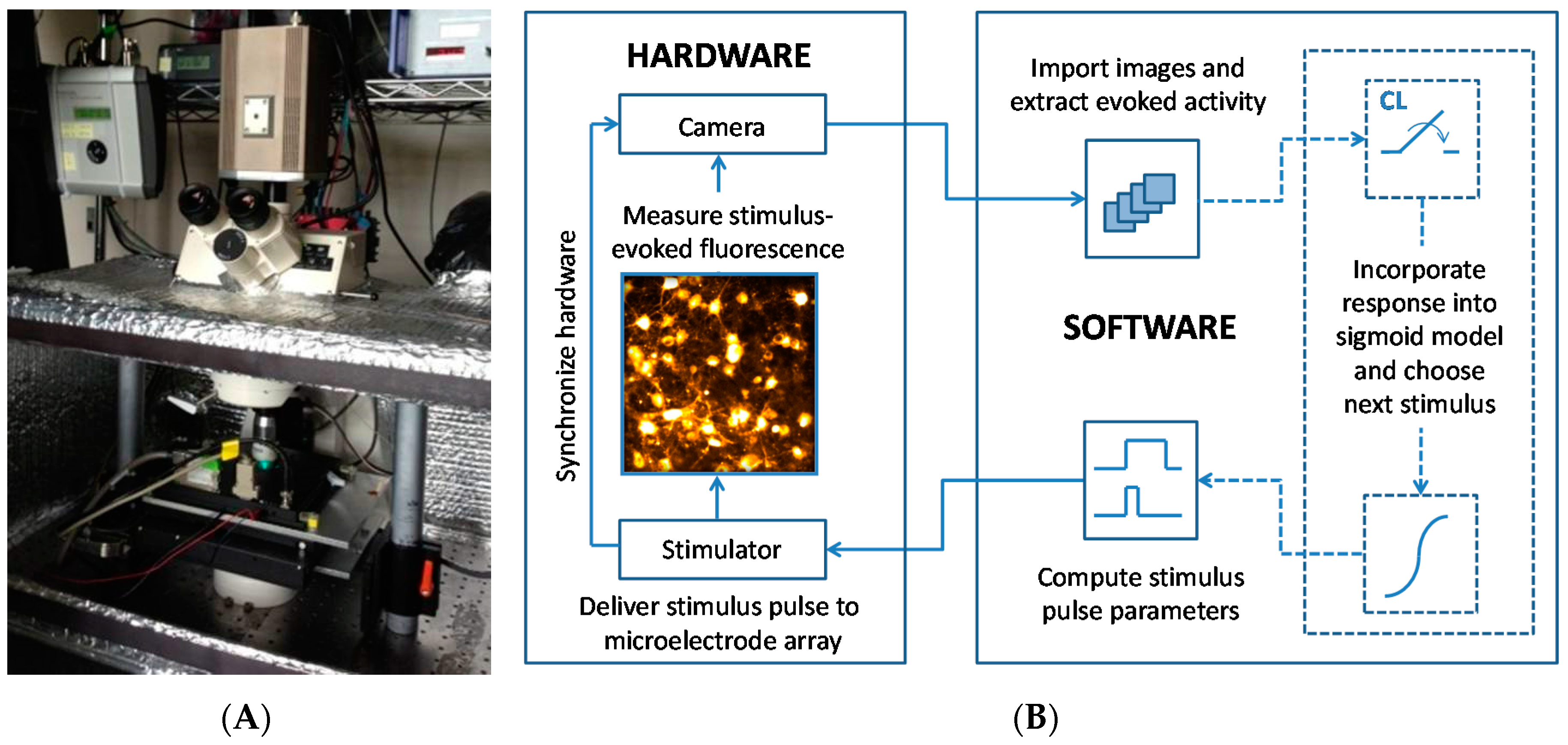
We designed a closed-loop system (Figure 1) for optimizing stimulus pulse parameters based on a model of neuronal activation and an experimental goal. The system comprises hardware and software components that select and deliver stimuli, which are designed to evoke a particular neuronal response. Each measured response is used to refine the model and the next stimulus is automatically chosen. The modular design, which separates data collection from both data analysis and decision-making, enables the user to plug in a model function and a variety of output measures to ask and answer a multitude of questions. Each section of the system is described in more detail below.

2.1. Cortical Cell Culture

Embryonic Day 18 (E18) rat cortices were enzymatically and mechanically dissociated according to [21]. Cortices were digested with trypsin (0.25% w/Ethylenediaminetetraacetic acid (EDTA)) for 10–12 min, strained through a 40 μm cell strainer to remove clumps and centrifuged to remove cellular debris. Neurons were re-suspended in culture medium (90 mL Dulbecco’s Modified Eagle’s Medium (Irvine Scientific 9024; Santa Ana, CA, USA), 10 mL horse serum (Life Technologies 1605, 0-122; Carlsbad, CA, USA), 250 μL GlutaMAX (200 mM; Life Technologies 35050-061), 1 mL sodium pyruvate (100 mM; Life Technologies 11360-070) and insulin (Sigma-Aldrich I5500; St. Louis, MO, USA; final concentration 2.5 μg/mL)) and diluted to 3000 cells/μL. Microelectrode arrays (MEAs; Multi Channel Systems 60MEA200/30iR-Ti; Kusterdingen, Germany) were sterilized by soaking in 70% ethanol for 15 min followed by UV exposure overnight. MEAs were treated with polyethylenimine to hydrophilize the surface, followed by three water washes and 30 min of drying. Laminin (10 μL; 0.02 mg/mL; Sigma-Aldrich L2020) was applied to the MEA for 20 min, half of the volume was removed, and 30,000 neurons were plated into the remaining laminin atop the MEA. Cultures were protected using gas-permeable lids [21] and incubated at 35 °C in 5% carbon dioxide and 95% relative humidity. The culture medium was fully replaced on the first DIV and then once every four DIV afterwards.

In these studies, Population A, comprised of 12 neurons, and Population B, comprised of 30 neurons, were grown atop a MEA with 30 μm diameter electrodes and 200 μm electrode spacing. Population C, comprising two neurons, was grown atop a MEA with 10 μm diameter electrodes and 30 μm electrode spacing.

2.2. Electrical Stimulation

Extracellular electrical stimuli were used to elicit neuronal activity. Stimuli were delivered to the neurons using a STG-2004 stimulator and MEA-1060-Up-BC amplifier (Multi Channel Systems). MATLAB (Natick, MA, USA) was used to control all hardware devices, which were synchronized by transistor-transistor logic (TTL) pulses sent from the stimulator at the beginning of each stimulation loop. In all stimulus iterations, a trigger pulse was first delivered to the camera to begin recording so that background fluorescence levels could be measured. An enable pulse was then delivered to the amplifier, which connected the stimulus channel to a pre-programmed electrode. A single cathodic square current pulse was then delivered to a single electrode centered under the camera field of view. Cathodic pulses were chosen because they have been shown to be most effective at evoking a neuronal response [22].

2.3. Optical Imaging

Automated optical imaging was used to measure the stimulus-evoked neuronal response. All preparation procedures were conducted in the dark to lengthen experiments by minimizing photobleaching and phototoxicity. Culture media was removed and neurons were loaded with Fluo-5F AM (Life Technologies F-14222), a calcium-sensitive fluorescent dye with relatively low binding affinity at a concentration of 9.1 μM in in DMSO (Sigma-Aldrich D2650), Pluronic F-127 (Life Technologies P3000MP) and artificial cerebral spinal fluid (aCSF; 126 mM NaCl, 3 mM KCl, 1 mM NaH₂PO₄, 1.5 mM MgSO₄, 2 mM CaCl₂, 25 mM d-glucose) with 15 mM 4-(2-hydroxyethyl)-1-piperazineethanesulfonic acid (HEPES) buffer for 30 min at ambient 25 °C and atmospheric carbon dioxide. Before imaging, cultures were rinsed two times with aCSF to remove free dye. Cultures were bathed in a mixture of synaptic blockers in aCSF (15 mM HEPES buffer). This included (2R)-amino-5-phosphonopentanoate (AP5; 50 μM; Sigma-Aldrich A5282), a NMDA receptor antagonist; bicuculline methiodide (BMI; 20 μM; Sigma-Aldrich 14343), a GABAA receptor antagonist; and 6-cyano-7-nitroquinoxaline-2,3-dione (CNQX; 20 μM; Sigma-Aldrich C239), an AMPA receptor antagonist. This mixture was shown to suppress neuronal communication [23] to ensure that the recorded neuronal activity was directly evoked by the stimulus. The culture was then kept in the heated amplifier (Multi Channel Systems TC02, 37 °C) within the imaging chamber. The stage position was calibrated with respect to the desired field of view (FOV) using the electrodes as fiducial markers. A MATLAB graphical user interface (GUI) was used to automatically position the FOV over the stimulation electrode. During an experiment neurons were illuminated using a light-emitting diode (LED; 500 nm peak power) and LED current source (TLCC-01-Triple LED; Prizmatix, Giv’at Shmuel, Israel) through a 20× immersion objective and a fluorescein isothiocyanate (FITC) filter cube. Evoked activity was optically recorded using a high-speed electron multiplication CCD camera (30 fps; QuantEM 512S; Photometrics, Tucson, AZ, USA), which has a 512 × 512 pixel grid covering a 400 μm × 400 μm area. After an experiment concluded, three aCSF washouts were performed at three minute intervals, the culture media was replaced, and the culture was returned to the incubator.

For each neuron, the measured intensity of 16 × 16 pixels (12.5 μm × 12.5 μm) surrounding the soma center was spatially averaged. The relative change in fluorescence, ΔF/F, was calculated by subtracting the baseline (an average of four pre-stimulus frames) from the peak (an average of four post-stimulus frames) and dividing the difference by the baseline. The standard deviation of the baseline frames was calculated in initial stimulus iterations and used as a measure of the fluorescence noise level. An action potential was said to have occurred if the ΔF/F was greater than three times the noise level within a particular neuron. The average decay time constant of a stimulus-evoked fluorescence curve was 1.5 s. Because of this relatively slow signal decay, the experiment loop time was chosen to be 4.5 s, which is three decay constants long, to give the signal sufficient time to return to baseline.

2.4. The Closed-Loop Search Algorithm and Activation Models

A saturating nonlinear curve was used to fit to the neuronal probability of firing an action potential in response to a varying stimulus current or pulse width. Specifically, a two-parameter model was used to describe this 1D activation curve for cathodic square-pulse stimuli:

$$p=\frac{1}{1+b_2{e}^{-\left(x-b_1\right)}}$$

(1)

The sigmoidal model provides an approximation for the stimulus needed to activate a particular neuron with any given probability. The input activation parameter, x, is either the stimulus current or pulse width, and the output is the probability, p, of a neuron to fire an action potential. The two parameters describing the sigmoid are b₁, the midpoint of the sigmoid, and b₂, the slope of the curve at the midpoint. Because the sigmoid describes a probability of activation, it spans from zero to one.

Sigmoidal activation curves are built to model neuronal activation along a one-dimensional cross section through the two-dimensional strength–duration waveform space. The closed-loop model-building search procedure begins with five open-loop (OL) stimuli that divides a one-dimensional cross section stimulation space evenly and brackets the activation region. After the fifth iteration, the sigmoidal model is analytically linearized, and a linear least-squares fit of the midpoint and slope parameters is performed. All measured stimulus-evoked responses are equally weighted. The output of the linear regression is used as an initial guess for a nonlinear least squares curve fit using the MATLAB Optimization Toolbox, which generates the best-fit sigmoid parameters. The measured response is a binomial distribution (a neuron either fired an action potential or it did not), and all points are equally weighted. In order to gain information about the sigmoid midpoint and slope parameters, a stimulus is chosen which lies along the transition region of the sigmoid. The stimulus that is predicted to produce a randomly selected target firing probability (e.g., 25%, 50%, 75%) is calculated analytically by inverting the sigmoid model. The probability goals span the linear portion of the transition region of the sigmoid curve, and an accurate measurement of the stimulus values at these probabilities provides an estimate of the slope of the curve at the midpoint. In the case that the next stimulus chosen was the same as the previously delivered stimulus, a uniformly random jitter was added to the stimulus up to 20% in either direction so that more data are collected over the full range of the transition region of the activation curve. After every stimulus iteration, the linear and nonlinear curve-fits are run to update the model.

During the CL search for a sigmoidal activation curve, stimuli were delivered along the transition region of the sigmoidal activation curve to improve the resolution of the model. While searching for the activation response data for a specific neuron, the CL routine simultaneously recorded activation response data for all other accessible neurons. For example, while the algorithm searched for the activation curve parameters for the Neuron 3 within a population of five neurons, it was continuously updating the model parameters for Neurons 1, 2, 4 and 5. The first five OL stimuli provided a model for all accessible neurons, abetted by a sparse representation. During the CL search routine, 30 stimuli were applied for each neuron, and when neuronal activation curves had similar thresholds, the data collected for one sigmoidal activation curve improved the resolution of the model for the similar neuron.

Neuronal activation in the 2D strength–duration waveform space was described according to Lapicque [24] and Weiss [25], which was developed in order to calculate the activation threshold, or the stimulus current needed to elicit a spike with 50% probability:

$$I=r\left(1+\frac{c}{PW}\right)$$

(2)

The stimulus pulse width, PW, is the input; the stimulus current, I, is the output, and the two model parameters are the rheobase, r, and the chronaxie, c, which describes the knee of the curve. The rheobase describes the stimulus current, below which a stimulus with infinite pulse width will not evoke an action potential, and the chronaxie describes the stimulus pulse width that corresponds to a stimulus current of twice the rheobase.

3. Results

We utilized the in vitro test bed to analyze the stimulus selectivity achievable using one- and two-parameter stimuli for three populations of neurons. In the first experiment, the stimulus selectivity achievable by varying a single input parameter was analyzed using Population A (n_A = 12 neurons). The stimulus pulse width was held constant while the stimulus current was varied in order to measure each neuronal activation curve. The one-parameter stimulus-evoked neuronal activation curves were uncovered using the closed-loop search strategy to model a neuronal activation curve and then deliver stimuli along the curve that are expected to reveal information regarding the transition region of the curve. After creating a model for each neuron’s activation, the distance in the stimulus current parameter space between the curves was measured. The second experiment was performed on Population B (n_B = 30 neurons) and focused first on understanding the spatial relationship between neuronal somata and the stimulating electrode. An open-loop stimulation strategy was used to construct two-parameter strength–duration models for all neurons in Population B by sweeping across all combinations of selected stimulus parameters. Once the 2D strength–duration activation models were created for Population B, the potential selectivity of a stimulus to activate one neuron and not another was analyzed. In the third study, we used the CL routine to measure activation curves for two neurons from multiple stimulating electrodes (Population C, n_C = 2 neurons). We again varied two stimulus parameters, however, and, in this experiment, the stimulus pulse width was held constant and the stimulating electrode location was varied by choosing a different planar electrode within the electrode array. In evaluating the stimulus selectivity between neurons, we found that we were able to differentially target our stimulus to particular neurons by exploiting the distribution of neuronal activation curves within the strength–duration waveform space on multiple electrodes.

3.1. Analysis of Selectivity with a One-Dimensional Input Space

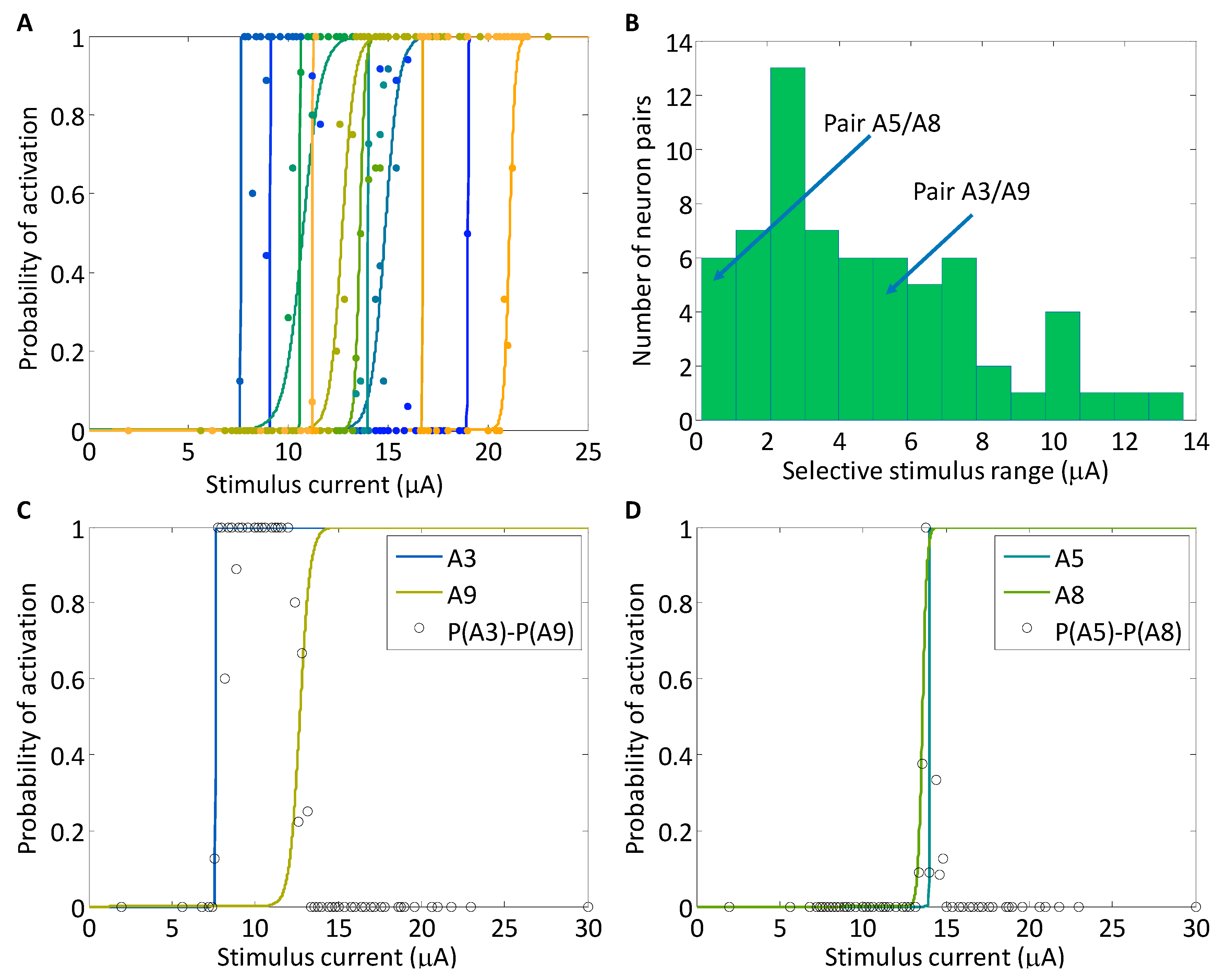
The sigmoidal activation curves for Population A were measured using the closed-loop search routine, and the stimulus pulse width was held constant at 800 μs during the searches. For each neuron, the activation of which was investigated one at a time, the CL search was terminated after 100 stimuli were delivered. The lowest activation threshold, defined as the midpoint of the sigmoid model, was 7.6 μA and the highest threshold was 21.1 μA, although the maximum stimulus current reached 30 μA. Of the twelve activation curves, seven curves lie within less than a 5 μA range from 10.6 μA to 14.8 μA (Figure 2A). We evaluated the stimulus selectivity that was achievable between neurons using the sigmoid activation curves. The selectivity range between a pair of neurons was defined as the stimulus distance between their thresholds, or sigmoid midpoints (Figure 2B). This metric was chosen because, at all points through the selectivity range, the neuron with a lower activation threshold will necessarily activate with probability greater than 0.5 and the neuron with the higher activation threshold will activate with probability less than 0.5. For neurons with vastly differing thresholds, there was a large stimulus range that was selective such that one neuron was exclusively activated. The largest selectivity range was between neurons A3 and A11 over a range of 13.7 μA. The selectivity is non-zero for all pairs of neurons, even along the transition region of the neuronal activation curves. We characterize neuron pairs into three classes of selectivity: highly selective (not shown), moderately selective (Figure 2C), and minimally selective (Figure 2D). For example, between Neurons A1 and A7, there was a highly selectivity range of 8.0 μA in which A7 activated while A1 was silent. Although the activation curve slope of Neuron A9 is shallower than that of other neurons, there is still a 6 μA selectivity range between Neurons A3 and A9 (Figure 2C). For neurons with relatively similar thresholds, as is the case of A5 and A8, selectivity remains non-zero. Even in this extreme example, despite minimal selectivity between the neurons, selectivity is still achievable: at the point 13.8 μA, A8 activated 100% of the time, while A5 never activated. Even at stimuli surrounding that point, there was a non-zero level of selectivity (Figure 2D).

The convergence of the sigmoid midpoint and slope had three phases. In the first 20 stimulus iterations, the slopes are nearly infinite because stimulus repetitions were not likely to be present until the algorithm had converged on the sigmoid midpoint. In this phase, the midpoint is fluctuating and the slope is infinite. For the next 20 stimulus iterations, the midpoints are relatively constant, and as the search routine selected the stimulus values predicted to produce firing probabilities of 0.25, 0.50 and 0.75, repetitions began to emerge. After 40 stimulus iterations, the algorithm has produced a good estimate of the sigmoid midpoint and slope, and time is spent refining those parameters. It is important to note that even after 100 stimulus iterations, the confidence interval, while stable, does not converge to zero. It will always be non-zero because the data comprise a binomial set, in which the least squares fitting algorithm will always fit zeroes and ones to a smooth probability curve. The experimental measurements taken along the slope of the curve, will, therefore, never overlay the actual curve, causing the confidence interval remain non-zero [26].

3.2. Analysis of Selectivity with a Two-Dimensional Input Space

We next analyzed the two-dimensional parameter space, combining stimulus strength (current) and pulse width (duration). To maximize the number of neurons that could be characterized in Population B, we used an open-loop stimulus routine to sweep a large range of stimulus currents and pulse-widths. This experiment delivered a randomized set of stimuli spanning currents from 2 μA to 20 μA in 1 μA increments and pulse-widths from 300 μs to 800 μs in 100 μs increments simultaneously to all neuron targets. One pulse was presented at a time, and ten repetitions of each pulse were delivered in random order throughout the experiment, yielding a 10% probability resolution at each stimulus parameter combination of current and pulse width. Action potentials were extracted, post hoc, to calculate action potential firing probabilities for each stimulus waveform. Sigmoidal activation curve models were constructed for each stimulus pulse width for all neurons, which entailed grouping the stimuli together with similar pulse width and then fitting the sigmoidal model to the range of stimulus currents. This then yielded a set of sigmoids (one for each stimulus pulse width) for each neuron. The sigmoidal models, each corresponding to a different stimulus pulse width, were used to predict the stimulus currents that would produce a probability estimate of 0.5 for each neuron so that strength–duration curves could be constructed. By using the sigmoidal models to predict probability points for each neuron at each delivered stimulus pulse width, the resulting data points (pulse-width in μs, strength in μA) were used as inputs into the SD model from Equation (2) to create p = 0.5 threshold curves for each of the 30 neurons (Figure 3A). We analyzed the two parameters used to describe the SD curve, chronaxie and rheobase, and note a trend that, as the rheobase increases, the chronaxie tends to decrease (Figure 3D).

We examined the spatial distribution of neuronal cell bodies in Population B within a 400 μm × 400 μm area across a range of neurons and stimulus pulse widths. A sigmoid activation curve was built for each neuron using the 300 μs and 800 μs pulse-width data, and the radial distance of the cell body from the stimulating electrode was calculated. Because the imaging methods employed here provided direct access to the radial soma-to-electrode distance, it was compared to the sigmoid model midpoint measured for each neuron individually (Figure 3B,C). As was the case for Population A, there was no observable correlation between the threshold and soma–electrode distance.

Neuronal activation probabilities were compared between the shortest and longest pulse-width data points collected—300 μs and 800 μs, respectively. Each of the 30 neurons of Population B is depicted by its 300 μs and 800 μs activation thresholds (Figure 3E), defined as the current levels at which a neuron fires an action potential with 0.5 probability. We manually selected two pairs of neurons with similar rheobase (B4, B21) or chronaxie (B19, B25) values. Selectivity is possible between these pairs of neurons because their thresholds reverse order from 300 μs to 800 μs. Neuron B19 has a higher activation threshold than B25 for the 300 μs pulse but has a lower activation threshold for the 800 μs pulse. Similarly, neuron B21 has a higher threshold than neuron B4 for the 300 μs pulse and vice versa at 800 μs. Graphically, this is seen as intersecting strength–duration activation curves (Figure 3F). When the SD curves intersect, the single stimulating electrode can be used to selectively activate neuron B4 over B21 and B25 over B19 at short stimulus pulse-widths and high stimulus currents. The opposite holds true for long stimulus pulse-widths and low currents.

3.3. Analysis of Selectivity with Multiple Electrodes

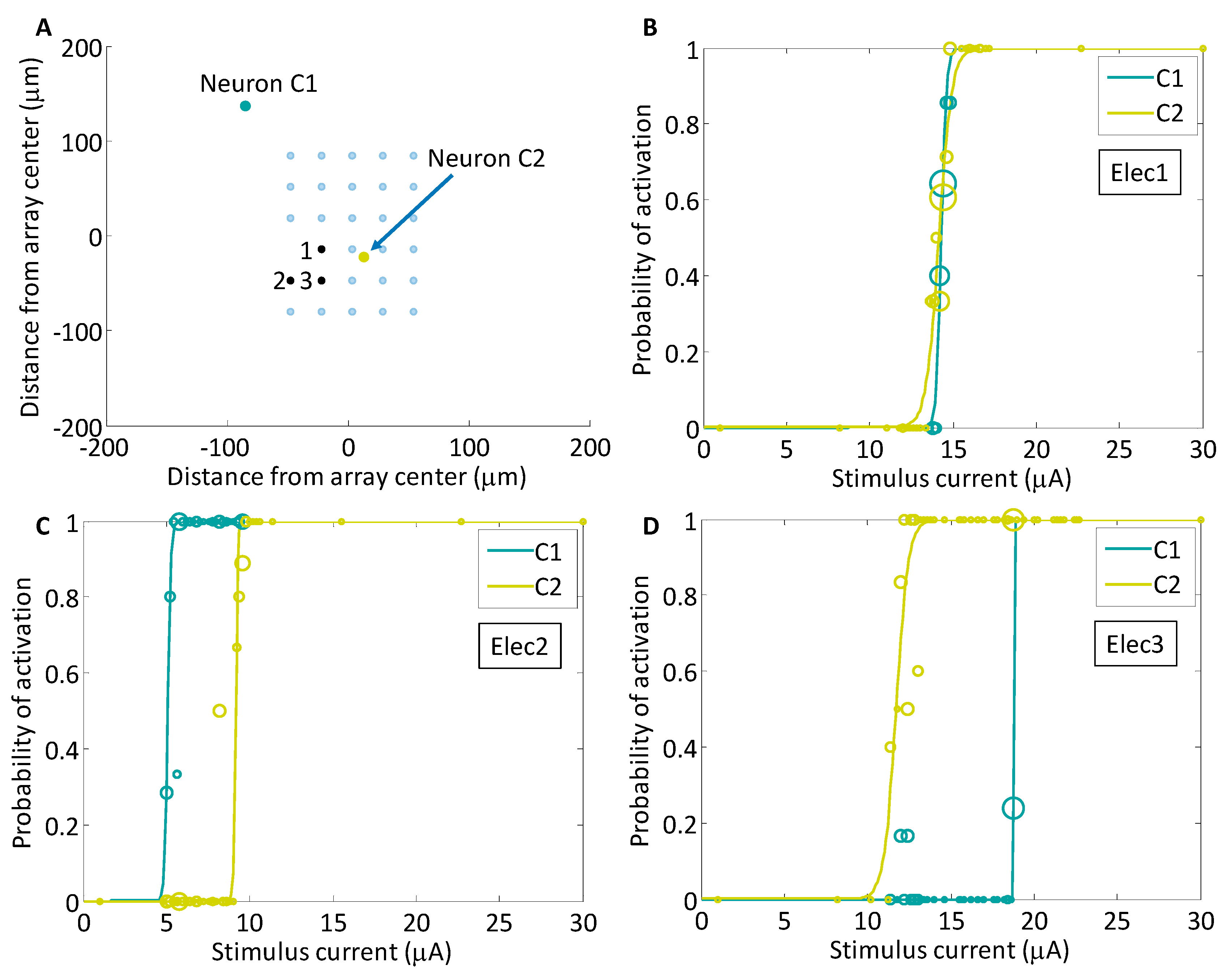
In the next set of experiments, we studied neuronal activation for two neurons using three electrodes. We constructed sigmoidal activation curves for the two neurons in Population C of the neuronal culture, which was grown on a high-density micro-electrode array (HD MEA), according to the CL search routine. A total of six sigmoidal activation curves were constructed for each neuron–electrode pair. The somata of Neurons C1 and C2 were at distances of 162 µm and 26 µm, respectively, from the center of the electrode array (Figure 4A). The activation curves for both neurons of interest were measured using Electrode 1. Neurons C1 and C2 had thresholds of 14.3 µA and 14.2 µA, and the transition regions spanned 0.4 µA and 0.9 µA (Figure 4B). Minimal selectivity is achievable for C2 at lower currents and for C1 at higher currents because these curves intersect. Nevertheless, the resulting selectivity is minimal because the activation curves are nearly overlapping. Next, the sigmoid activation curve measurement was repeated from Electrode 2. Using Electrode 2, C1 and C2 had activation thresholds of 5.1 µA and 9.2 µA and transition regions spanning 0.2 µA and 0.1 µA, respectively (Figure 4C). The stimulus current range that was selective for C1 was measured as the current distance between the midpoints of the activation curves and spanned 4.1 µA. Finally, when Electrode 3 was used, the activation curves for Neurons C1 and C2 reversed order. C1 and C2 had activation thresholds of 18.8 µA and 11.7 µA (Figure 4D). The transition region for C1 was less than 0.2 µA and for C2 was 0.8 µA. The selective current range for C2 spanned 7.1 µA.

4. Discussion

Effective waveform design is integral in improving the selectivity and control of neuronal stimulation systems. Altering the stimulus amplitude (current or voltage) is the most frequently used method for waveform modification; this approach is inherently limited in its selectivity as it typically activates many axons within a region [15,27]. Control of the stimulus amplitude is an essential element but is insufficient for differential activation of neurons within a population using a single electrode. Expanding the one-dimensional approach to multidimensional waveforms applied to multiple neurons facilitates the development of targeted stimulation technologies.

4.1. Adaptive Targeted Searches Can Find Even a Small Window for Selectivity

We have shown that even for similar neuronal activation curves, when the apparent selectivity achievable was minimal, such as between A5 and A8 (Figure 2D), it remained non-zero. The CL routine was used to measure each neuronal activation curve; however, it could be adapted to target specific selectivity regions between neuronal pairs. By searching for the maximum of the difference of sigmoids, the CL search routine could be used to find the 13.8 μA stimulus current, which would enable the targeting of Neuron A8. The use of an optimized CL routine for searching the multi-parameter space additionally enhanced the ability to find stimuli enabling the reversal of selectivity between neurons (Figure 4C,D). Additionally, the CL routine could be optimized for many other stimulation goals, including finding the most selective stimulus range to divide the population or stimulate two neurons and not another. A combination of the two techniques, using closed-loop searches to find the optimal stimulus, and then searching in a multi-parameter stimulus space, we can quickly locate the relevant stimulus waveform subspace. An array of stimulating electrodes could be used to further increase selectivity. The opportunity for reversing the activation curves between a pair of neurons expands when increasing the parameter space to include spatially distributed electrodes.

Other metrics could be used to describe the selectivity between neurons, depending on the end goal. As an example, if the target metric is to first minimize the activation of A5, the previous definition of selectivity, which finds the range over which the difference in the activation probabilities is greater than 0.5, could be sacrificed to ensure with higher probability that A5 did not activate. A lower stimulus current could be delivered in the range of 13.4–13.6 μA, where although there is a limited probability of activating A8, the probability of activating A5 is significantly lower. The selectivity may also be defined as the integral of the area between the activation curves.

4.2. Probing of the Population Response Is Essential for Targeted Stimulation

From Figure 3B, it can be inferred that there is no apparent relationship between soma location and activation threshold. Numerous modeling and experimental studies focus on the activation of neurons and their elements in response to electrical stimulation. These studies show that axons are most susceptible to stimulation, which can explain the vast spatial distribution of activated neuronal somata in response to an extracellular stimulus [15,27,28,29,30]. Knowledge of the location of neuronal somata within a tissue volume is insufficient to determine the threshold at which a particular population of neurons will activate. Due to the complex spatial organization of neuronal cultures and networks, implanted electrodes or planar electrode arrays will have access to many different locations along many different axons. Additionally, electrode locations and neuronal populations are unique: what may work in one neuronal environment may fail in another. The natural variability in electrode locations and neuronal populations demands that for each application the stimulus-evoked response in the reachable populations is rapidly probed and characterized. The inability to precisely locate an electrode array in a neuronal culture requires that a neural stimulator be functionally evaluated via targeted stimulation. If a functional map may be constructed, the practical need for precise spatial mapping of electrodes and axons is unnecessary.

In the experimental application, there is variability in the cell numbers, absolute cell position, and location of the cells relative to the micro-electrode arrays (MEA). This high variability will similarly apply to clinical applications, given natural patient-to-patient variability. It must therefore be assumed that each experimental or clinical application will have a unique response. It is the uniqueness of each application that requires that the accessible neuronal population be learned, and this accessible population be probed for response in the stimulus parameter space. Feedback is required in this system because, as is shown in this work and others [29], there is no apparent correlation between cell distance from the electrode and stimulus response. In our experimental system, we use widefield optical imaging as a measurement tool; it is likely in a clinical application that non-optical methods will be used to record evoked activity. The findings in this work are independent of measurement method, and so also apply to non-optical recording methods. Ultimately, any stimulation routine needs to implement a technique to probe and characterize the population response in order to design targeted stimuli that will enable more sophisticated control of the evoked response.

4.3. Using an Array of Spatially Distributed Electrodes

In a repetition of the multi-electrode experiment from Figure 4, we characterized neuronal activation for two neurons using seven stimulating electrodes. Six showed activation preference for one neuron, while the other one allowed access to selectively stimulate the second neuron. There is no guarantee that a pair of adjacent electrodes will enable reversible selectivity between a pair of neurons, which emphasizes the need for a method that utilizes the full extent of the accessible electrodes within the array for finding the best stimulating electrode for a particular goal. More specifically, a fast closed-loop search routine is required because it is unknown, a priori, which electrodes will provide access to which neurons.

Based on the activation data in Figure 4, we hypothesize that the axon of C1 is directed downward and the axon of C2 is directed to the left (oriented as shown on Figure 4A). It is possible that both axons traverse the array such that the most excitable elements pass equidistant from Electrode 1 because their activation thresholds are similar. The axon of Neuron C1 is likely positioned closer to stimulating Electrode 2 than that of Neuron C2 because it activates with a lower current, and conversely, the axon of Neuron C2 is likely closer to stimulating Electrode 1 than that of Neuron C1. The observations of this experiment underscore that an array of electrodes be used in selective stimulation so that multiple electrodes are available for stimulation and may be selected based on the stimulation goals. Access to multiple electrode locations, with respect to the underlying tissue, provides greater access to selectivity between neurons.

4.4. As the Parameter Space Increases, CL Systems Behave More Similarly to OL Systems

There is a constraint on the number of stimulus trials that may be presented, due to the need for efficient alleviation of symptoms, in a clinical environment, and due to photobleaching and phototoxicity, in the experimental setting presented here. For this reason, if 30 stimuli per neuron are required and only the stimulus current or pulse-width is of experimental interest, a CL routine is preferred for up to approximately 20 neurons. The number of neurons for which this CL method is preferable decreases when the dimension of the stimulus parameter space increases because more stimuli are required to build a multi-dimensional model for each neuron. An OL stimulation approach becomes superior when a large population of neurons must be described, as in the case of the 30 neuron experiments in Population B. It is also notable that, even with a CL approach, for a sufficient number of neurons (ca. 10), the aggregation of all the CL searches becomes similar to an OL approach because the stimuli cover a similar area. The CL routine has a distinct advantage when the activation curves are close in proximity; in these cases, the stimuli delivered to uncover one activation curve is simultaneously increasing the resolution of the activation probability measurement for another neuron. As the stimulus space increases with more neurons, more waveform parameters, or more electrodes, the set of CL searches will eventually tend toward an OL sweep. Despite this tendency, the CL approach reduces inefficiencies in the OL routine, including eliminating the delivery of stimuli at the lowest currents or shortest pulse-widths. Further improvements in efficiency can be made to make the CL routine more adaptive by allowing the CL routine to terminate early if neuronal activation curves are similar to one another, reducing the number of stimuli necessary for subsequent neurons.

5. Conclusions

Selectivity between two neurons is achievable using a single electrode. For a single stimulus parameter search, in either current or pulse-width, even for neurons with very similar activation transition regions, a CL technique can find the stimulus waveform that is able to selectively activate the lower threshold neuron. This selectivity is assured, however, only for the lower threshold neuron. For this reason, it is important that the full stimulus waveform space be exploited to differentially target neurons. Two-way selectivity is sometimes achievable between pairs of neurons using only a single stimulating electrode, but it is limited to those pairs in which the strength–duration curves cross one another. The organization of the culture with respect to the stimulating electrode can be functionally measured in real-time to assess the achievable selectivity. Additionally, it is essential that the multi-parameter activation space be initially measured so that the delivered stimuli can then be optimized for improving the efficiency with which a population activation probability is measured. The techniques developed here can be used to improve the selectivity of a stimulus waveform by simultaneously stimulating on multiple electrodes, which enables a reversible selectivity.

References

- Clark, K.L.; Armstrong, K.M.; Moore, T. Probing neural circuitry and function with electrical microstimulation. Proc. R. Soc. B Biol. Sci. 2011, 278, 1121–1130. [Google Scholar] [CrossRef] [PubMed]
- Borchers, S.; Himmelbach, M.; Logothetis, N.; Karnath, H.O. Direct electrical stimulation of human cortex—The gold standard for mapping brain functions? Nat. Rev. Neurosci. 2011, 13, 63–70. [Google Scholar] [CrossRef] [PubMed]
- Joucla, S.; Branchereau, P.; Cattaert, D.; Yvert, B. Extracellular neural microstimulation may activate much larger regions than expected by simulations: A combined experimental and modeling study. PLoS ONE 2012, 7, e41324. [Google Scholar] [CrossRef] [PubMed]
- Jun, S.B.; Smith, K.L.; Shain, W.; Dowell-Mesfin, N.M.; Kim, S.J.; Hynd, M.R. Optical monitoring of neural networks evoked by focal electrical stimulation on microelectrode arrays using FM dyes. Med. Biol. Eng. Comput. 2010, 48, 933–940. [Google Scholar] [CrossRef] [PubMed]
- Newman, J.P.; Zeller-Townson, R.; Fong, M.F.; Desai, S.A.; Gross, R.E.; Potter, S.M. Closed-loop, multichannel experimentation using the open-source NeuroRighter electrophysiology platform. Front. Neural Circuits 2013, 6, 98. [Google Scholar] [CrossRef] [PubMed]
- Franke, F.; Jäckel, D.; Dragas, J.; Müller, J.; Radivojevic, M.; Bakkum, D.; Hierlemann, A. High-density microelectrode array recordings and real-time spike sorting for closed-loop experiments: An emerging technology to study neural plasticity. Front. Neural Circuits 2012, 6, 105. [Google Scholar] [CrossRef] [PubMed]
- Müller, J.; Bakkum, D.J.; Hierlemann, A. Sub-millisecond closed-loop feedback stimulation between arbitrary sets of individual neurons. Front. Neural Circuits 2012, 6, 121. [Google Scholar] [CrossRef] [PubMed]
- Nicolas, J.; Hendriksen, P.J.; van Kleef, R.G.; de Groot, A.; Bovee, T.F.; Rietjens, I.M.; Westerink, R.H. Detection of marine neurotoxins in food safety testing using a multielectrode array. Mol. Nutr. Food Res. 2014, 58, 2369–2378. [Google Scholar] [CrossRef] [PubMed]
- Valdivia, P.; Martin, M.; LeFew, W.R.; Ross, J.; Houck, K.A.; Shafer, T.J. Multi-well microelectrode array recordings detect neuroactivity of ToxCast compounds. Neurotoxicology 2014, 44, 204–217. [Google Scholar] [CrossRef] [PubMed]
- Jankowska, E.; Roberts, W.J. Synaptic actions of single interneurones mediating reciprocal Ia inhibition of motoneurones. J. Physiol. 1972, 222, 623–642. [Google Scholar] [CrossRef] [PubMed]
- Jensen, R.J.; Ziv, O.R.; Rizzo, J.F., III; Scribner, D.; Johnson, L. Spatiotemporal aspects of pulsed electrical stimuli on the responses of rabbit retinal ganglion cells. Exp. Eye Res. 2009, 89, 972–979. [Google Scholar] [CrossRef] [PubMed]
- Sekirnjak, C.; Hottowy, P.; Sher, A.; Dabrowski, W.; Litke, A.M.; Chichilnisky, E.J. Electrical stimulation of mammalian retinal ganglion cells with multielectrode arrays. J. Neurophysiol. 2006, 95, 3311–3327. [Google Scholar] [CrossRef] [PubMed]
- Yeomans, J.S.; Maidment, N.T.; Bunney, B.S. Excitability properties of medial forebrain bundle axons of A9 and A10 dopamine cells. Brain Res. 1988, 450, 86–93. [Google Scholar] [CrossRef]
- Bostock, H. The strength-duration relationship for excitation of myelinated nerve: Computed dependence on membrane parameters. J. Physiol. 1983, 341, 59–74. [Google Scholar] [CrossRef] [PubMed]
- Nowak, L.G.; Bullier, J. Axons, but not cell bodies, are activated by electrical stimulation in cortical gray matter. Exp. Brain Res. 1998, 118, 477–488. [Google Scholar] [CrossRef] [PubMed]
- Dziubińska, H.; Paszewski, A.; Trębacz, K.; Zawadzki, T. Electrical activity of the liverwort Conocephalum conicum: The all-or-nothing law, strength-duration relation, refractory periods and intracellular potentials. Physiol. Plant. 1983, 57, 279–284. [Google Scholar] [CrossRef]
- Fozzard, H.A.; Schoenberg, M. Strength-duration curves in cardiac Purkinje fibres: Effects of liminal length and charge distribution. J. Physiol. 1972, 226, 593–618. [Google Scholar] [CrossRef] [PubMed]
- McIntyre, C.C.; Grill, W.M. Extracellular stimulation of central neurons: Influence of stimulus waveform and frequency on neuronal output. J. Neurophysiol. 2002, 88, 1592–1604. [Google Scholar] [PubMed]
- Boinagrov, D.; Loudin, J.; Palanker, D. Strength–duration relationship for extracellular neural stimulation: Numerical and analytical models. J. Neurophysiol. 2010, 104, 2236–2248. [Google Scholar] [CrossRef] [PubMed]
- Edelstein, A.; Amodaj, N.; Hoover, K.; Vale, R.; Stuurman, N. Computer control of microscopes using μManager. Curr. Protoc. Mol. Biol. 2010, 14, 14–20. [Google Scholar]
- Potter, S.M.; DeMarse, T.B. A new approach to neural cell culture for long-term studies. J. Neurosci. Methods 2001, 110, 17–24. [Google Scholar] [CrossRef]
- Wagenaar, D.A.; Pine, J.; Potter, S.M. Effective parameters for stimulation of dissociated cultures using multi-electrode arrays. J. Neurosci. Methods 2004, 138, 27–37. [Google Scholar] [CrossRef] [PubMed]
- Bakkum, D.J.; Chao, Z.C.; Potter, S.M. Long-term activity-dependent plasticity of action potential propagation delay and amplitude in cortical networks. PLoS ONE 2008, 3, e2088. [Google Scholar] [CrossRef] [PubMed]
- Lapicque, L. Quantitative investigations of electrical nerve excitation treated as polarization. 1907. Biol. Cybern. 2007, 97, 341–349. [Google Scholar] [PubMed]
- Weiss, G. Sur la possibilite de rendre comparables entre eux les appareils servant a l’excitation electrique. Arch. Ital. Biol. 1901, 35, 413–446. [Google Scholar]
- Cox, D.R. The regression analysis of binary sequences. J. R. Stat. Soc. Ser. B (Methodological) 1958, 20, 215–242. [Google Scholar]
- Tehovnik, E.J.; Tolias, A.S.; Sultan, F.; Slocum, W.M.; Logothetis, N.K. Direct and indirect activation of cortical neurons by electrical microstimulation. J. Neurophysiol. 2006, 96, 512–521. [Google Scholar] [CrossRef] [PubMed]
- Ranck, J.B., Jr. Which elements are excited in electrical stimulation of mammalian central nervous system: A review. Brain Res. 1975, 98, 417–440. [Google Scholar] [CrossRef]
- Histed, M.H.; Bonin, V.; Reid, R.C. Direct activation of sparse, distributed populations of cortical neurons by electrical microstimulation. Neuron 2009, 63, 508–522. [Google Scholar] [CrossRef] [PubMed]
- Rattay, F. The basic mechanism for the electrical stimulation of the nervous system. Neuroscience 1999, 89, 335–346. [Google Scholar] [CrossRef]
Figure 1.
The open-loop and closed-loop system of electrical stimulation, optical recording, automated image analysis and activation curve modeling. (A) A photograph of the system apparatus is shown. The camera is mounted atop the microscope with an inline piezoelectric actuator connected to the 20× objective for high-precision focal plane adjustments. LED fluorescence excitation is digitally controlled, eliminating the need for a shutter. The neuronal culture lives atop the microelectrode array (MEA), which is nested inside of the heated Multi Channel Systems preamplifier. Imaging is carried out inside of an enclosure to eliminate ambient light exposure and reduce the effects of other environmental factors including the laboratory heating and ventilation. The preamplifier is housed inside of this “light tight” imaging chamber and interfaces with the external stimulator. (B) Hardware for delivering electrical stimuli and for optically recording evoked responses (left) interfaces directly with the MATLAB-based software system (MATLAB 7.12, The MathWorks Inc., Natick, MA, USA, 2011) (right). The open-loop experimental configuration is depicted with solid arrows. Predefined stimulus pulse parameters are sent to the stimulator for delivery to the MEA. The stimulator supplies synchronizing triggers to the camera, LED, and preamplifier. Fluorescence is evoked at cell somata that fire action potentials in response to the stimulus. This fluorescence signal is captured by the camera with a series of high-speed digital frames. The set of frames is imported into MATLAB and saved to the hard disk using the Micro-Manager library [20]. In the closed-loop configuration (dotted lines), the neuronal response is used to inform the calculation of the next iteration of stimulus pulse parameters. Digital images are analyzed using custom software to extract stimulus-evoked action potentials. This newly acquired response data is compiled with previous stimulus iterations and the sigmoid activation model is updated to reflect all measured responses. The next stimulus pulse is then chosen to increase the measurement resolution along the slope of the response curve.
Figure 2.
(A) The closed-loop routine was used to measure neuronal activation curves for Population A in the stimulus current space while the stimulus pulse width was fixed. Each activation curve describes the probability of a neuron to fire an action potential across a range of stimulus currents. The curves are arbitrarily shaded to aid in viewing the lines. For each curve, there are similarly shaded probability points lying along the curve, which describe the average firing probability for a neuron at a particular stimulus current. (B) The selectivity achievable between all possible pairs within Population A is depicted in a histogram. The selective stimulus range is calculated as the absolute value of the difference in the p = 0.5 points for each pair of neurons. For all pairs of neurons, the selectivity is non-zero. (C,D) Two pairs of neuronal activation curves (solid lines) are depicted. For each stimulus current, the difference in neuronal activation (open circles) was calculated by subtracting the two probabilities of firing. This difference in probabilities is a measure of the selectivity of the stimulus between the two neurons and was calculated directly from the data. (C) The selectivity achievable between A3 and A9 spanned 5 μA. (D) For the pair of neurons, A5 and A8, although the activation curves lie close to one another, there is a stimulus point at 13.8 μA, where A8 is activated and A5 is not.
Figure 3.
(A) Strength–duration curves for Population B span a large range of the stimulus-pulse parameter space. These curves are described by the rheobase, or the stimulus current threshold at infinite pulse-width, and the chronaxie, or the stimulus pulse-width at twice the rheobase current. Intuitively, these parameters define the horizontal asymptote and the knee of the curve. The vertical dotted line represents the 300 μs cross section. (B) The spatial location with respect to the stimulating electrode (open circle in the center) of all 30 neuronal somata is depicted within the imaging plane. Each soma is shaded according to its activation threshold for a 300 μs stimulus pulse width. (C) For the same neurons, the radial distance of the soma to the electrode is shown versus the activation threshold for both 300 μs and 800 μs pulse widths. Twelve neurons lie between 150 μm and 200 μm away from the electrode, radially, and have activation thresholds that span a 14 μA range of currents for the 300 μs pulse-width data and 10 μA for the 800 μs pulse-width data. (D) The distribution of rheobase and chronaxie parameters is shown for Population B. Four neurons are highlighted. (E) Each of the 30 neurons from Population B is depicted by its 300 μs and 800 μs activation thresholds, which are the current levels at which a neuron fires an action potential half of the time. The same four neurons are highlighted from the previous figure. These neuron pairs reverse threshold order from 300 μs to 800 μs. Neuron B19 has a higher threshold than B25 for the 300 μs pulse, but has a lower threshold for the 800 μs pulse. (F) The strength–duration activation curves are plotted for the four neurons highlighted in (E). Each pair of neurons (B19/B25 and B4/B21) has curves that cross one another. Because of this crossing, this single stimulating electrode can be used to selectively activate Neuron B4 over B21 and Neuron B25 over B19 at short stimulus pulse-widths and high stimulus currents. The opposite holds true for long stimulus pulse-widths and low currents.
Figure 4.
(A) The physical locations of the two neurons in Population C are depicted. The three stimulating electrodes used (10 µm diameter, 30 µm spacing) are numbered (black circles). Neurons C1 (dark circle) and C2 (light circle) are located 162 µm and 26 µm, radially, from the center of the array. (B–D) The activation curves found using the CL algorithm for two neurons, C1 (dark shade) and C2 (light shade), are depicted with solid lines. The measurement of the activation probability for each neuron in response to all stimuli delivered are shown with open circles, with the circle radius in proportion to the number of stimuli delivered at that point. (B) The activation curves for both Neurons C1 and C2 found using Electrode 1. The largest open circle along the activation curve of neuron C1 is depicts 29 stimulus responses. (C) The activation curves for both Neurons C1 and C2 found using Electrode 2, and (D), the activation curves for both Neurons C1 and C2 found using Electrode 3.
© 2017 by the authors. Licensee MDPI, Basel, Switzerland. This article is an open access article distributed under the terms and conditions of the Creative Commons Attribution (CC BY) license (http://creativecommons.org/licenses/by/4.0/).
Share and Cite
MDPI and ACS Style
Kuykendal, M.L.; Potter, S.M.; Grover, M.A.; DeWeerth, S.P. Targeted Stimulation Using Differences in Activation Probability across the Strength–Duration Space. Processes 2017, 5, 14. https://doi.org/10.3390/pr5020014
AMA Style
Kuykendal ML, Potter SM, Grover MA, DeWeerth SP. Targeted Stimulation Using Differences in Activation Probability across the Strength–Duration Space. Processes. 2017; 5(2):14. https://doi.org/10.3390/pr5020014
Chicago/Turabian StyleKuykendal, Michelle L., Steve M. Potter, Martha A. Grover, and Stephen P. DeWeerth. 2017. "Targeted Stimulation Using Differences in Activation Probability across the Strength–Duration Space" Processes 5, no. 2: 14. https://doi.org/10.3390/pr5020014
Note that from the first issue of 2016, this journal uses article numbers instead of page numbers. See further details here.