Structural Properties of Dynamic Systems Biology Models: Identifiability, Reachability, and Initial Conditions

Abstract

Dynamic modelling is a powerful tool for studying biological networks. Reachability (controllability), observability, and structural identifiability are classical system-theoretic properties of dynamical models. A model is structurally identifiable if the values of its parameters can in principle be determined from observations of its outputs. If model parameters are considered as constant state variables, structural identifiability can be studied as a generalization of observability. Thus, it is possible to assess the identifiability of a nonlinear model by checking the rank of its augmented observability matrix. When such rank test is performed symbolically, the result is of general validity for almost all numerical values of the variables. However, for special cases, such as specific values of the initial conditions, the result of such test can be misleading—that is, a structurally unidentifiable model may be classified as identifiable. An augmented observability rank test that specializes the symbolic states to particular numerical values can give hints of the existence of this problem. Sometimes it is possible to find such problematic values analytically, or via optimization. This manuscript proposes procedures for performing these tasks and discusses the relation between loss of identifiability and loss of reachability, using several case studies of biochemical networks.

1. Introduction

The study of parametric identifiability is a fundamental task of system identification, which can be approached from structural or practical viewpoints [1,2,3]. Practical identifiability analysis aims at characterizing the uncertainty in parameter estimates taking into account the deficiencies in the data used for model calibration. Structural identifiability is a prerequisite for practical identifiability, and seeks to establish whether the model parameters can be uniquely determined from observations of the input-output behaviour of the model—that is, from the model equations only. The concept of structural identifiability was coined in [4] and initially introduced in the context of linear systems. It was soon extended to the nonlinear case and many methods were subsequently developed for its study [3,5,6]. In parallel, the classic dual concepts of observability and controllability were also extended from linear [7] to nonlinear [8]. The relationships between these properties make it natural to study structural identifiability with the tools of nonlinear observability [9]. Indeed, it is possible to check simultaneously the observability and structural identifiability of a model by including its parameters in the state variables vector, and calculating the rank of the resulting (augmented) observability matrix. Several computational methods that build on this idea have been presented in the last decade [10,11,12,13].

However, the results of these methods should be taken with caution. As emphasized by Denis-Vidal et al. [14], identifiability may depend on the initial conditions. Saccomani et al. [15] noted that differential algebra methods can incorrectly classify an unidentifiable model as identifiable for certain initial conditions (a detailed distinction between “structural”, “geometric”, and “algebraic” identifiability can be found in [16]).

Here we show that the differential geometry approach (which assesses local structural identifiability by checking the rank of the augmented observability matrix) has in principle the same limitation as the differential algebra approach with regard to initial conditions. When the identifiability matrix is computed with the numerical values of certain problematic initial conditions, its rank decreases with respect to the general case. However, this situation cannot be detected with symbolic rank calculations. When the system evolves from such initial conditions it may become impossible—depending on the particular case—to determine some of its parameters, which would nevertheless be structurally identifiable if the system was started at a different state. In [15] loss of reachability was identified as the cause of this loss of identifiability. However, other alternative causes may also exist. To assess this possibility we propose to check if the identifiability rank condition is satisfied in two ways: for the generic case (symbolically), and in the vicinity of the initial conditions of interest (by specializing its states to those specific values). By performing the rank test both for generic and particular state values we obtain a more complete diagnosis. Then, if a certain numerical state vector leads to an incomplete identifiability rank, it may indicate that some state variables are no longer reachable from it, which in turn may make the associated parameters unidentifiable. This situation can be checked by assessing the reachability of the system both for generic and particular states—or, alternatively, by simulating the model using the state vector as initial condition. This procedure allows to determine precisely if the parameters are structurally locally identifiable for those values. An alternative solution could be to check identifiability in a range of parameter and state values, as proposed by [11], although the computational complexity of such test makes it infeasible for medium or large-scale systems. Given that, in general, the identifiability condition may be misleading when evaluated for generic values of the states, an important question is whether it is possible to determine the specific values that violate this test. For small models it may be possible to find them analytically by inspection of the system equations. In more complex cases an alternative is to search for such values via optimization.

The organization of this paper is as follows: in Section 2 we provide a compact presentation of the necessary background on structural identifiability, observability, and reachability (controllability) of nonlinear systems, and of the relations between these concepts. When available, necessary and/or sufficient conditions under which these properties hold are given. This is presented using the differential geometry formulation. Then in Section 3 we illustrate with six example models several situations and issues that can appear in relation to loss of structural identifiability, and how this relates to observability and reachability. We begin in Section 3.1 by remembering the known fact that reachability is neither necessary nor sufficient for identifiability. Then in Section 3.2 we show that identifiability rank tests can sometimes (i.e., for certain state vectors) be misleading. We further remark, in Section 3.3, that the knowledge of initial conditions of unmeasured states can improve the identifiability. In Section 3.4 we propose a procedure that assesses whether the identifiability rank test is being misleading, and in Section 3.5 we propose an optimization-based procedure to find particular state vectors will cause loss of identifiability. Finally, we summarize the Conclusions in Section 4.

2. Background: Nonlinear Observability, Reachability, and Identifiability

2.1. Notation and Differential Geometry Concepts

We consider a general class of nonlinear time-invariant systems modelled as a structure M with the following dynamic equations:

$$M:\left\{\begin{array}{c}\dot{x}\left(t\right)=f(x,p,u)=f_1(x,p)+f_2(x,p)·u\left(t\right)\hfill \\ y\left(t\right)=h(x,p)\hfill \\ x_0=x(t=0,p)\hfill \end{array}\right.$$

(1)

where f, $f_1$, $f_2$, and h are vector functions, $p\in {\mathbb{R}}^q$ is a real-valued vector of parameters, $u\in {\mathbb{R}}^r$ is the input vector, $x\in {\mathbb{R}}^n$ the state variable vector, and $y\in {\mathbb{R}}^m$ the output or observables vector. The dependency of $f,f_1,f_2$, and h on the parameters p will be usually dropped for ease of notation. The following paragraphs define several differential geometry concepts that will be used throughout this paper.

Given a smooth function $z\left(x\right)$ and a vector field $v\left(x\right)$, the Lie derivative of z with respect to v is:

$$L_{v}z\left(x\right)=\frac{\partial z\left(x\right)}{\partial x}v\left(x\right)$$

(2)

where $\frac{\partial }{\partial x}z\left(x\right)$ is a row vector containing the partial derivatives of the smooth function $z\left(x\right)$. In the present work, $z\left(x\right)$ can be either the m-dimensional vector function $h\left(x\right)$ (when studying observability) or the r-dimensional vector function $f_2\left(x\right)$ (when studying controllability). For a k-dimensional function z and an n-dimensional vector x and function v, $\frac{\partial }{\partial x}z\left(x\right)$ is a $k\times n$ matrix, and $L_{v}z\left(x\right)=\frac{\partial z\left(x\right)}{\partial x}v\left(x\right)$ is a $k\times 1$ column vector. Higher order Lie derivatives can be defined recursively as:

$$\begin{array}{c}\hfill \begin{array}{ccc}\hfill L_v^{2}z\left(x\right)& =& \frac{\partial L_{v}z\left(x\right)}{\partial x}v\left(x\right)\hfill \\ \cdots \\ \hfill L_v^{i}z\left(x\right)& =& \frac{\partial L_v^{i-1}z\left(x\right)}{\partial x}v\left(x\right)\hfill \end{array}\end{array}$$

(3)

Given two vector fields $v_1\left(x\right),v_2\left(x\right)$, their Lie bracket is the vector field defined by

$$[v_1,v_2]=\frac{\partial v_2}{\partial x}{v}_1-\frac{\partial v_1}{\partial x}{v}_2$$

(4)

A $k-$dimensional distribution$\Delta$ on X is a map which assigns, to each $x\in X$, a $k-$dimensional subspace of ${\mathbb{R}}^n$ such that for each $x_0\in X$ there exist an open set $U\subseteq X$ containing $x_0$ and k vector fields $f_1,\cdots ,f_k$, such that

• $\{f_l\left(x\right),\cdots ,f_k\left(x\right)\}$ is a linearly independent set for each $x\in U$.
• $\Delta \left(x\right)=\mathbf{span}\{f_1\left(x\right),\cdots ,f_k\left(x\right)\}$, $\forall x\in U$ [17].

2.2. Observability

Conceptually, a system is observable if for each state there exists at least one input which allows to discriminate between this state and all nearby states, by measuring the output [17]. More formally, two states $x_0\ne x_1$ are said to be distinguishable when there exists some input $u\left(t\right)$ such that $y(t,x_0,u\left(t\right))\ne y(t,x_1,u\left(t\right))$, where $y(t,x_i,u\left(t\right))$ denotes the output function of the system for the input $u\left(t\right)$ and initial state $x_i(i=0,1)$. The system is said to be (locally) observable at $x_0$ if there exists a neighbourhood N of $x_0$ such that every other $x_1\in N$ is distinguishable from $x_0$.

2.2.1. Linear Observability

Before proceeding to nonlinear systems, let us recall that a linear system of the form

$$\begin{array}{c}\hfill \begin{array}{ccc}\hfill \dot{x}& =& A·x+B·u\hfill \\ \hfill y& =& C·x\hfill \end{array}\end{array}$$

(5)

is observable if and only if $\mathrm{rank}\left(\mathcal{O}\right)=n$, where $\mathcal{O}$ is the linear observability matrix [7,

$$\begin{array}{c}\hfill \mathcal{O}\left(x\right)=\left(\begin{array}{c}C\\ C·A\\ C·A^2\\ ⋮\\ C·A^{n-1}\end{array}\right)\end{array}$$

(6)

2.2.2. Nonlinear Observability

The extension to the nonlinear case is straightforward. For a system given by (1), the nonlinear observability matrix is built using Lie derivatives as follows:

$$\begin{array}{c}\hfill \mathcal{O}\left(x\right)=\left(\begin{array}{c}\frac{\partial }{\partial x}h\left(x\right)\\ \frac{\partial }{\partial x}\left(L_{f}h\left(x\right)\right)\\ \frac{\partial }{\partial x}\left(L_f^{2}h\left(x\right)\right)\\ ⋮\\ \frac{\partial }{\partial x}\left(L_f^{n-1}h\left(x\right)\right)\end{array}\right)\end{array}$$

(7)

Theorem 1. Observability Rank Condition (ORC).

If the system M given by (1) satisfies $\mathit{rank}\left(\mathcal{O}\left(x_0\right)\right)=n$, where $\mathcal{O}$ is defined by (7), then M is locally observable around $x_0$ [8].

The ORC is a sufficient and “almost necessary” condition for observability [17], meaning that if M is locally observable around $x_0$, then $\mathrm{rank}\left(\mathcal{O}\left(x_0\right)\right)=n$ for all the states belonging to an open dense subset of the state space. Note that, in passing from linear to nonlinear, the rank condition has changed from being sufficient and necessary to being “sufficient and almost necessary”.

Two terms related to observability are detectability and reconstructability. Detectability is a similar notion to observability, but slightly weaker: a system is detectable if all the unstable modes are observable. Reconstructability is also similar, but it refers to the ability of determining the present state of a system from past and current (as opposed to future) measurements.

2.3. Controllability and Reachability

While observability studies whether it is possible to reconstruct the internal state x of a model by observing its output y, controllability asks whether it is possible to control x by manipulating its input u. Controllability and reachability are subtly different concepts: in reachability the question is which states $x\left(t_f\right)$ can be reached in finite time from the initial state, $x\left(t_0\right)$, which is fixed. In controllability the question is which states $x\left(t_0\right)$ can be driven to a final state, $x\left(t_f\right)$, which is fixed. A more precise definition of reachability is as follows: a system (1) is said to be (locally) reachable around a state $x_0$ if there exists a neighbourhood N of $x_0$ such that, for each $x_f\in N$, there exist a time $T>0$ and a set of inputs u such that, if the system starts in state $x_0$ at time $t=0$, it reaches $x_f$ at time $t=T$. It should be noted that for nonlinear systems, the possibility of reaching from any given state a set of full dimension has also been called weak (local) controllability [8] and accessibility [18]. Here, following [17], we will refer to it as nonlinear reachability or simply reachability.

2.3.1. Linear Controllability and Reachability

A linear system given by (5) is reachable if and only if $\mathrm{rank}\left(\mathcal{C}\right)=n$, where $\mathcal{C}$ is the linear controllability matrix defined as:

$$\mathcal{C}\left(x\right)=\left(B|A·B|A^2·B|\cdots |A^{n-1}·B\right)$$

(8)

While the condition $\mathrm{rank}\left(\mathcal{C}\right)=n$ is both sufficient and necessary for reachability, for controllability it is only sufficient; that is, if A is singular, the system may be controllable even if $\mathrm{rank}\left(\mathcal{C}\right)<n$.

The “duality” between observability and controllability/reachability can be noticed by inspecting the linear observability (6) and controllability (8) matrices, since:

$$\begin{array}{c}\hfill \begin{array}{c}rank\left(B|A·B|A^2·B|\cdots |A^{n-1}·B\right)=n\iff \hfill \\ \iff rank\left(\begin{array}{c}{B}^T\\ B^T·A^T\\ B^T·{\left(A^T\right)}^2\\ ⋮\\ B^T·{\left(A^T\right)}^{n-1}\end{array}\right)=n\hfill \end{array}\end{array}$$

(9)

Thus, the pair $(A,B)$ is reachable if and only if the pair $(A^T,B^T)$ is observable.

2.3.2. Nonlinear Controllability and Reachability

The nonlinear controllability matrix of the system (1) is as follows:

$$\begin{array}{c}\hfill \mathcal{C}\left(x\right)=\left(\begin{array}{ccccc}{f}_2\left(x\right)& L_{f_1}{f}_2\left(x\right)& L_{f_1}^2{f}_2\left(x\right)& \cdots & L_{f_1}^{n-1}{f}_2\left(x\right)\end{array}\right)\end{array}$$

(10)

The controllability matrix can be used to determine reachability with the following theorem:

Theorem 2. Controllability Rank Condition (CRC).

If the system M given by (1) satisfies $\mathit{rank}\left(\mathcal{C}\left(x_0\right)\right)=n$, then M is (locally) reachable in a neighbourhood $N\left(x_0\right)$ of $x_0$ [17].

Note that the CRC is a conservative criterion, since it provides only a sufficient—but not necessary—condition for reachability. A necessary condition can be obtained from the so-called controllability distribution ${\Delta }_c\left(x\right)$, which is computed iteratively as a sequence of distributions:

$${\Delta }_0=\mathrm{span}\left\{f_2\right\}\to {\Delta }_1\to {\Delta }_2\to \dots \to {\Delta }_{n-1}={\Delta }_c,$$

(11)

with the following recursive rule:

$${\Delta }_{i+1}=\mathrm{span}\left\{{\Delta }_i\bigcup \left\{[f_1,q],[f_2,q]:q\left(x\right)\in {\Delta }_i\left(x\right)\right\}\right\}$$

(12)

Theorem 3. Reachability Theorem.

The system M given by (1) is (locally) reachable around $x_0$ if and only if there exists a neighbourhood N of $x_0$ such that the distribution ${\Delta }_c\left(x\right)$, constructed as in (11,12), has constant dimension n for all $x\in N$ [17].

While Theorem 3 provides a necessary and sufficient condition, it is more difficult to check than the CRC.

2.4. Structural Identifiability as Observability

Assuming that the model structure M (1) is correct, that the data is noise-free, and that the inputs to the system can be chosen freely, it is always possible to choose an estimated parameter vector $\widehat{p}$ such that the model output $h(x,\widehat{p})$ equals the one obtained with the true parameter vector, $h(x,p^{*})$. If $\widehat{p}=p^{*}$ this is trivially the case.

A parameter $p_i$ is structurally locally identifiable if for almost any $p^{*}\in \mathbb{R}$ there is a neighbourhood $N\left(p^{*}\right)$ such that

$$\widehat{p}\in N\left(p^{*}\right)\mathrm{and}h(x,\widehat{p})=h(x,p^{*})\Rightarrow \widehat{p_i}=p_i^{*}$$

(13)

A model M is structurally locally identifiable (s.l.i.) if all its parameters are s.l.i. If (13) does not hold in any neighbourhood of $p^{*}$, parameter $p_i$ is structurally unidentifiable. A model M is structurally unidentifiable if at least one of its parameters is structurally unidentifiable.

Identifiability analysis can be formulated as a nonlinear observability problem [9,19]. To do so, let us augment the state variable vector so as to include also the model parameters:

$$\begin{array}{c}\hfill \tilde{x}=\left[\begin{array}{c}x\\ p\end{array}\right]\end{array}$$

(14)

Accordingly, the f function that describes the time evolution of the state variables in equation (1) is augmented as follows:

$$\begin{array}{c}\hfill \tilde{f}\left(\tilde{x}\right)=\left[\begin{array}{c}\dot{x}\\ \dot{p}\end{array}\right]=\left[\begin{array}{c}f(x,u)\\ 0\end{array}\right]\end{array}$$

(15)

where 0 is a zero-valued (since the parameters are constant in time) column vector of dimension $q\times 1$.

The resulting generalized observability-identifiability matrix, $O_I\left(\tilde{x}\right)$, can be written as:

$$\begin{array}{c}\hfill {\mathcal{O}}_I\left(\tilde{x}\right)=\left(\begin{array}{c}\frac{\partial }{\partial \tilde{x}}h\left(\tilde{x}\right)\\ \frac{\partial }{\partial \tilde{x}}\left(L_{\tilde{f}}h\left(\tilde{x}\right)\right)\\ \frac{\partial }{\partial \tilde{x}}\left(L_{{\tilde{f}}^2}h\left(\tilde{x}\right)\right)\\ ⋮\\ \frac{\partial }{\partial \tilde{x}}\left(L_{{\tilde{f}}^{n+q-1}}h\left(\tilde{x}\right)\right)\end{array}\right)\end{array}$$

(16)

where $L_{\tilde{f}}h\left(\tilde{x}\right)$ is a Lie derivative defined as in equation (2), that is, $L_{\tilde{f}}h\left(\tilde{x}\right)=\frac{\partial h\left(\tilde{x}\right)}{\partial \tilde{x}}\tilde{f}\left(\tilde{x}\right)$, and higher order derivatives are defined recursively as in equation (3).

Theorem 4. Observability-Identifiability Condition (OIC).

If M given by (1) satisfies $\mathit{rank}\left({\mathcal{O}}_I\left({\tilde{x}}_0\right)\right)=n+q$, then M is (locally) observable and identifiable in a neighbourhood $N\left({\tilde{x}}_0\right)$ of ${\tilde{x}}_0$.

Proof. 

It follows immediately from Theorem 1 and the definition of $\tilde{x}$. ☐

3. Results

Here we discuss the relationships between the structural properties defined in Section 2 and some issues that may appear. We illustrate them with several case studies, which are listed in

Table 1. Main properties of the examples used in this paper. The term “generic” applied to SI (structural identifiability) or reachability means that the model has said property for almost all values of x. The last three columns refer to the possibility of losing said properties for certain values of x. N/A stands for Not Applicable.

Example	Ref.	(Generic)	(Generic)	Decrease	Loss	Loss of
		SI	Reachability	in rank(${\mathit{O}}_{\mathit{I}}$)	of SI	Reachability
1	This paper	YES	NO	NO	NO	N/A
2	This paper	NO	YES	N/A	N/A	NO
3	[23]	NO	YES	N/A	N/A	YES
4	[11]	YES	NO	YES	YES	N/A
5	[24]	YES	NO	YES	NO	N/A
6.A	[14]	NO	NO	N/A	N/A	N/A
6.B	[14]	YES	NO	YES	NO	N/A

along with a summary of their properties.

3.1. Reachability Is Neither Necessary Nor Sufficient for Identifiability

For linear systems it was established early on that, despite the relationships that exist between those properties, observability and controllability are neither necessary nor sufficient conditions for structural identifiability. This was noted by DiStefano [20] by providing simple counter-examples (although DiStefano’s brief note was disputed, see [21,22] and the author’s replies to those comments). In a similar way, this section shows by means of three small examples that, for nonlinear systems, reachability—or lack thereof—has in principle no implications for structural identifiability.

Example 1.

A model that is structurally identifiable but unreachable:

$$M_1:\left\{\begin{array}{c}\dot{x_1}=p_1·(x_1^2+A),\hfill \\ \dot{x_2}=p_2·(x_1·x_2+B)+u,\hfill \\ y_1=x_1,\hfill \\ y_2=x_2\hfill \end{array}\right.$$

(17)

where $\{p_1,p_2\}$ are unknown parameters and $\{A,B\}$ known constants, all of which are positive quantities. The controllability distribution of $M_1$ is

$$\begin{array}{c}\hfill {\Delta }_c\left(x\right)=\mathrm{span}\left\{\begin{array}{cc}0& 0\\ 1& -p_2·x_1\end{array}\right\}\end{array}$$

(18)

which has dimension $1<n=2$, so $M_1$ is unreachable (Theorem 3). Its observability-identifiability matrix is

$$\begin{array}{c}\hfill {\mathcal{O}}_I\left(\tilde{x}\right)=\left(\begin{array}{cccc}1& 0& 0& 0\\ 0& 1& 0& 0\\ 2·p_1·x_1& 0& x_1^2+A& 0\\ p_2·x_2& p_2·x_1& 0& x_1·x_2+B\end{array}\right)\end{array}$$

(19)

which has $\mathrm{rank}\left({\mathcal{O}}_I\left(\tilde{x}\right)\right)=4=n+q$, which means that it is observable and identifiable (OIC).

Example 2.

A model that is structurally unidentifiable but reachable:

$$M_2:\left\{\begin{array}{cc}\dot{x_1}\hfill & =p_1·x_1·x_2^2+u,\hfill \\ \dot{x_2}\hfill & =p_2·x_1,\hfill \\ y\hfill & =p_3·x_1\hfill \end{array}\right.$$

(20)

The controllability distribution of $M_2$ is

$$\begin{array}{c}\hfill {\Delta }_c\left(x\right)=\mathrm{span}\left\{\begin{array}{cc}1& -p_1·x_2^2\\ 0& -p_2\end{array}\right\}\end{array}$$

(21)

which has dimension 2, so $M_2$ is reachable (Theorem 3). It is straightforward to calculate ${\mathcal{O}}_I\left(\tilde{x}\right)$ (not shown here due to its large size) and see that $\mathrm{rank}\left({\mathcal{O}}_I\left(\tilde{x}\right)\right)=3<n+q=5$, which means that it is unidentifiable (OIC). Specifically, $p_2$ is identifiable but $p_1$ and $p_3$ are not. It can also be noticed that, according to the classic definition of observability (which assumes that the parameter values are known) model $M_2$ is observable, since

$$\begin{array}{c}\hfill \mathcal{O}\left(x\right)=\left(\begin{array}{cc}1& 0\\ p_1·x_2^2& 2·p_1·x_1·x_2\end{array}\right)\end{array}$$

(22)

and thus $\mathrm{rank}\left(\mathcal{O}\right(x\left)\right)=2$ and the ORC holds.

Example 3.

A model that is structurally unidentifiable but (almost everywhere) reachable:

$$M_3:\left\{\begin{array}{cc}{\dot{x}}_1\hfill & =p_1·x_1·x_2,\hfill \\ {\dot{x}}_2\hfill & =p_2·u,\hfill \\ y\hfill & =x_1\hfill \end{array}\right.$$

(23)

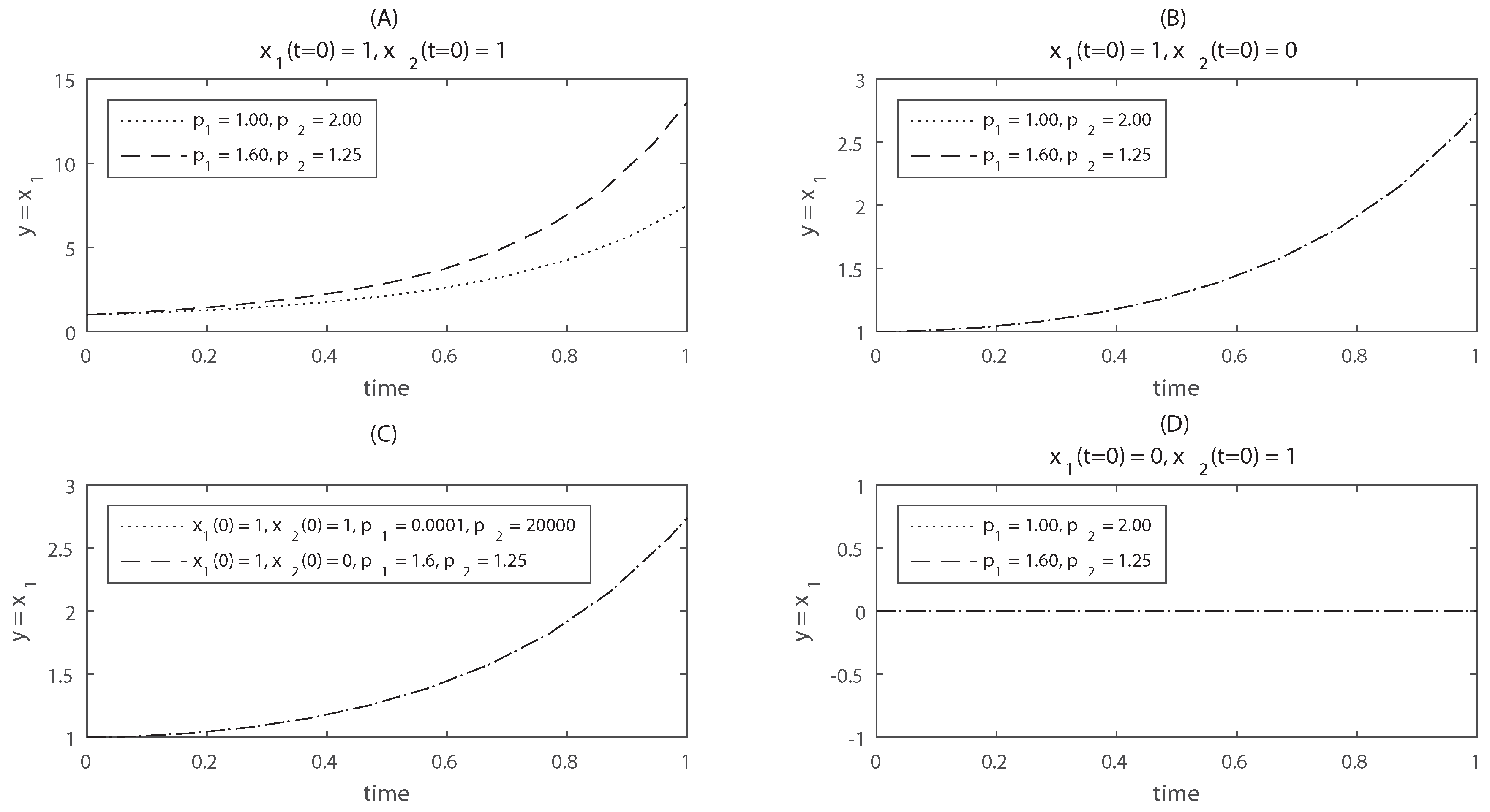
This model is taken from [23]. For this system $n+q=4$ and $\mathrm{rank}\left(O_I\left(\tilde{x}\right)\right)=3$. Thus the observability-identifiability condition (OIC) of Theorem 4 does not hold; the model as a whole, and $\{p_1,p_2\}$ in particular, are structurally locally unidentifiable. This unidentifiability result was obtained symbolically, for generic values of the initial conditions. To illustrate this lack of identifiability, the time evolution of $M_3$ is shown in Figure 1 for two different parameter vectors: $\{p_1=1,p_2=1\}$ and $\{p_1=1.6,p_2=1.25\}$. If the model is simulated from the initial conditions $\{x_1\left(0\right),x_2\left(0\right)\}=\{1,1\}$, the model outputs are distinguishable for the two different parameter vectors (panel A). However, when the model is simulated from $\{x_1\left(0\right),x_2\left(0\right)\}=\{1,0\}$, the outputs are identical (panel B): for these initial conditions the parameters are indistinguishable, i.e., the model is unidentifiable. Furthermore, even if the model is started from a different initial condition, $x_2\ne 0$, its output may be the same to that of $x_2=0$ for two different parameter vectors (panel C). Thus, the structural unidentifiability of this model is not exclusive of the initial condition $x_2=0$. Note that, however, if we were able to measure not only $x_1$ but also $x_2$, the model would become identifiable, since the time course of $x_2$ is different in each of the aforementioned cases.

Regarding reachability, the controllability distribution of $M_3$ is

$$\begin{array}{c}\hfill {\Delta }_c\left(x\right)=\mathrm{span}\left\{\begin{array}{cc}0& -p_1·p_2·x_1\\ p_2& 0\end{array}\right\}\end{array}$$

(24)

which has dimension 2, so $M_3$ is reachable (Theorem 3). Thus, $M_3$ is generically reachable and structurally unidentifiable. So is $M_2$; however, there is a difference between both models: unlike in the case of $M_2$, the dimension of the controllability distribution of $M_3$ can decrease for certain values of x: specifically, for $x_1=0$, its dimension decreases from 2 to 1, as can be seen in Equation (24), and in that particular case the model is no longer reachable. This is illustrated in panel D of Figure 1, which shows that if $x_1\left(0\right)=0\Rightarrow x_1\left(t\right)=0\forall t$. We remark that this loss of reachability is not the cause of the model’s unidentifiability, since the model is also unidentifiable for the initial conditions shown in the other panels, for which there is no loss of reachability.

3.2. The Results of Identifiability Tests Can Be Misleading for Certain State Vectors

The OIC of Theorem 4 represents a general result, which is valid for all values of the states and parameters except for a set of measure zero. For these exceptions, however, its results may be misleading. This section illustrates this fact with an example.

Example 4.

A structurally identifiable model that loses identifiability for certain values of x:

Consider the following biochemical network [11]:

$$E+S\underset{p_2}{\stackrel{p_0}{\rightleftarrows }}ES\stackrel{p_3}{\to }E+P;P\stackrel{p_1}{\to }\varnothing$$

(25)

If we denote by $x_1$, $x_2$, and $x_3$ the concentrations of substrate (S), enzyme (E), and product (P), respectively, this system can be modelled by the following equations [11]:

$$M_4:\left\{\begin{array}{c}{\dot{x}}_1=-x_1·x_2+p_2·(10-x_2),\hfill \\ {\dot{x}}_2=-x_1·x_2+(p_2+p_3)·(10-x_2),\hfill \\ {\dot{x}}_3=-p_1·x_3+p_3·(10-x_2)\hfill \\ y_1=x_1,y_2=x_3\hfill \end{array}\right.$$

(26)

Note that these equations were obtained by August and Papachristodoulou [11] after making two assumptions: (i) that $\left[ES\right]+\left[E\right]=10$, which allows omitting [ES] from the equations by replacing it with $\left[ES\right]=10-\left[E\right]=10-x_2$; and (ii) that the reaction rates are normalized, such that $p_0=1$ is a known constant.

For this example $n+q=6$ and $\mathrm{rank}\left(O_I\left(\tilde{x}\right)\right)=6$, which means that the OIC of Theorem 4 holds. Therefore methods based in the OIC [10,11,13] classify the model as observable and identifiable for generic values of the states and parameters. However, note that for the particular initial conditions $\{x_1\left(0\right)=0,x_2\left(0\right)=10\}$, two of the states remain at zero $\{x_1\left(t\right)=0,x_2\left(t\right)=0\}\forall t\ge 0$, and in this case only $p_1$ appears in the equations. Thus, for these particular initial conditions the model is not identifiable, since it is not possible to determine the values of $p_2$ and $p_3$. Obviously, model $M_4$ is not reachable, since it does not have any control inputs and thus its controllability distribution is empty. Therefore the loss of identifiability cannot be attributed to a loss of reachability for certain initial conditions. However, it is linked to the fact that $\{x_1,x_2\}$ remain equal to zero if the system is started from $\{x_1\left(0\right)=0,x_2\left(0\right)=10\}$. This situation is not rare: indeed, by examining the Equation (17) that describe model $M_1$, it can be noticed that if $A=0$, state $x_1$ would remain equal to zero if started in that condition, and the model would be unidentifiable, since the third column of its observability-identifiability matrix (19) would be zero.

Example 4 shows how a model that is “generally” structurally identifiable—that is, it is identifiable for almost all values of its state variables—can lose its identifiability for certain particular values of its states (or equivalently, for certain initial conditions). This loss of identifiability results from some of the states of $M_4$ remaining at zero value from certain initial conditions, which prevents some parameters appearing in the equations of those states from being identified. This loss of identifiability causes a loss of rank in the OIC: if the model states are replaced with the initial conditions of interest, $x_0*$, it results that $\mathrm{rank}\left(O_I(x_0*)\right)<n+q$; thus the loss of identifiability entails a rank deficiency.

However, this rank check is not a definitive proof: the next model provides a counter-example that shows that, even when the rank of a (generally structurally identifiable) matrix decreases for certain initial conditions, this does not necessarily result in structural unidentifiability.

Example 5.

A structurally identifiable model despite rank deficiency of $O_I$ for certain values of x:

Robertson [24] proposed as a case study an autocatalytic reaction with the following scheme:

$$x_1\stackrel{k_1}{\to }{x}_2;2x_2\stackrel{k_2}{\to }{x}_2+x_3;x_2+x_3\stackrel{k_3}{\to }{x}_1+x_3$$

(27)

Its kinetics are given by the following equations:

$$M_5:\left\{\begin{array}{c}{\dot{x}}_1=-k_1·x_1+k_3·x_2·x_3,\hfill \\ {\dot{x}}_2=k_1·x_1-k_2·x_2^2-k_3·x_2·x_3,\hfill \\ {\dot{x}}_3=k_2·x_2^2\hfill \\ y_1=x_1,y_2=x_2\hfill \end{array}\right.$$

(28)

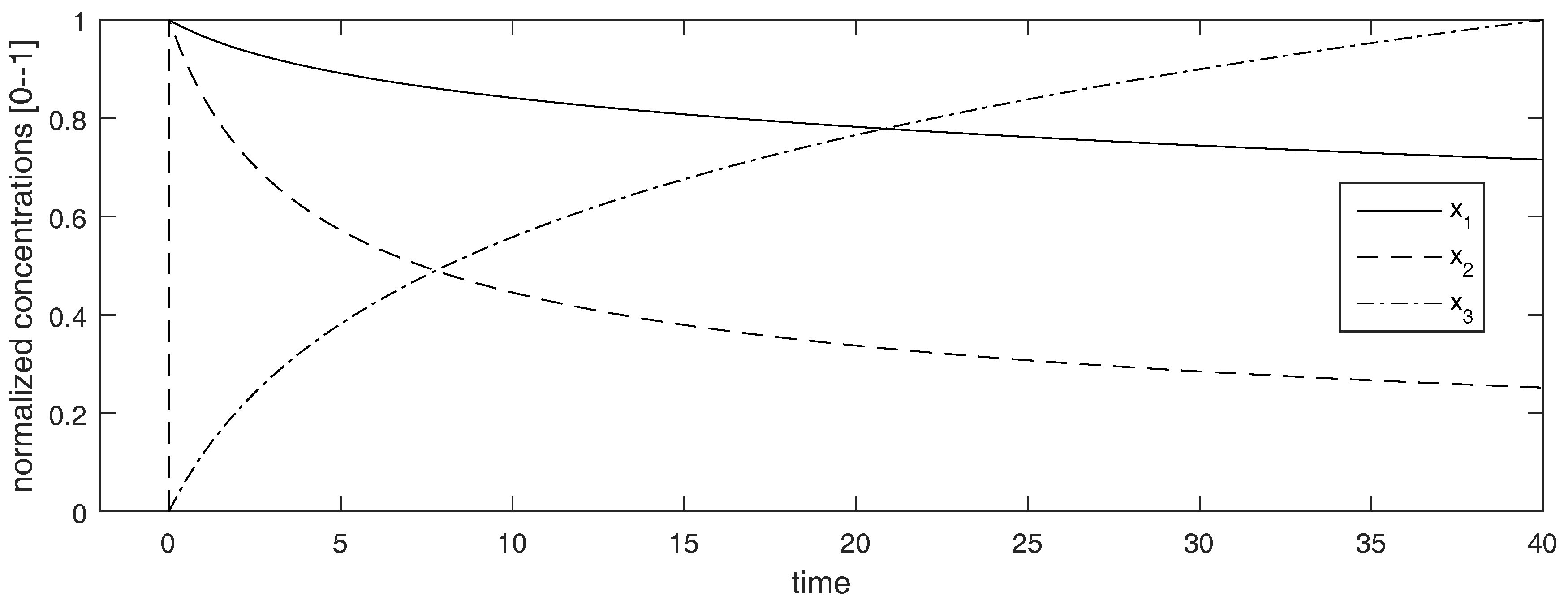
This model was showcased in [25] as an example of an unidentifiable model, and later used as a case study in [26]. Specifically, Eydgahi et al. stated that “the inability of estimation to recover the parameter values used to generate synthetic data is not due to problems with the computational procedures. Instead, it represents a fundamental limit on our ability to understand biochemical systems based on time-course data alone”. However, this model is in fact structurally identifiable ($O_I$ is full rank for generic values of x), although its practical identifiability is poor. A reason for its lack of practical identifiability is that, for the nominal parameter values, $x_2$ has very low values compared to the other two states (six orders of magnitude smaller). Thus, the difficulty in recovering the true values of its parameters is not due to a structural deficiency, but to numerical limitations.

Interestingly, when $x_2\left(0\right)=x_3\left(0\right)=0$, the observability-identifiability matrix $O_I$ is not full rank, so the system may seem to be structurally unidentifiable from those initial conditions. However, such a loss of identifiability is “strictly local”. By this we mean that, as can be seen in Figure 2, all the states (including $x_2$ and $x_3$) reach non-zero values immediately after $t=0$ (note that the concentration curves have been normalized to adopt values between 0 and 1, to facilitate the visualization). For example, at $t=10$ the state vector is $\{x_1\left(10\right)=0.8414,x_2\left(10\right)=1.623·{10}^{-5},x_3\left(10\right)=0.1586\}$, and $O_I$ has full rank when evaluated at that point. Therefore the model is still identifiable when simulated from these initial conditions. This example shows that, even when the $O_I$ loses its full rank for certain values of the state variables, this does not necessarily lead to loss of identifiability, as long as it does not produce loss of accessibility.

3.3. Knowledge of Additional Initial Conditions Can Increase Identifiability

So far we have assumed that the initial conditions of the states corresponding to measured outputs are known, and that those of unmeasured states are unknown. This is the typical situation: in general we do not have information about unmeasured states; on the other hand, since structural identifiability analysis assumes unlimited measurements, we can consider all the values of the measured states known—including, naturally, their initial conditions.

However, in certain cases we may possess information about the initial condition of a state, even if we are not able to measure its subsequent behaviour. In this case, such additional information can help identify some parameters that would be unidentifiable without it. This possibility was noted by Chappell and Godfrey [27], who used a case study which they claimed to be the first example of a real-life nonlinear model that was not globally identifiable. Here we illustrate this case with the following example:

Example 6.

A structurally unidentifiable model that becomes identifiable if the initial conditions (of unobserved states) are known:

Denis-Vidal et al [14] proposed the following model to illustrate how the identifiability of uncontrolled models may depend on the initial conditions.

$$M_6:\left\{\begin{array}{c}{\dot{x}}_1={\theta }_1·x_1^2+{\theta }_2·x_1·x_2,x_1\left(0\right)=1\hfill \\ {\dot{x}}_2={\theta }_3·x_1^2+x_1·x_2,x_2\left(0\right)=b\hfill \\ y=x_1\hfill \end{array}\right.$$

(29)

It can be seen that parameters ${\theta }_2$ and ${\theta }_3$ are structurally unidentifiable; we refer to this case as Example 6.A (as written in Table 1). However, if we know the initial condition of the unmeasured state, $x_2\left(0\right)=b$, then the model becomes structurally identifiable; we refer to this variant as Example 6.B. In this case, a decrease in the rank of $O_I$ (from full rank, 5, to 4) takes place if $b=0$, but, similarly to Example 5, the state $x_2$ immediately departs from zero and the model is structurally identifiable.

3.4. Guaranteeing the Results of the Structural Identifiability Test

The examples of the preceding section show that local structural identifiability is a generic property that may be lost for particular values of the state variables, and that such loss of identifiability may not be detected by differential geometry methods such as those based on the OIC. This issue is shared by differential algebra methods: for them, [15,28] concluded that the result of the identifiability test is still correct if a model is globally inaccessible (unreachable), but problems appear when a model is only inaccessible from initial points belonging to a thin set.

The realization in [15,28] suggests performing an additional check on the reachability of a system: if for a certain state $x_0$ we find both a decrease in the rank of the observability-identifiability matrix $O_I\left(x_0\right)$ and a decrease in the dimension of the controllability distribution ${\Delta }_c\left(x_0\right)$, we can conclude that the model is not identifiable when started from the initial conditions $x_0$. However, there are issues that cannot be revealed by this test: we have seen that such a loss of identifiability for particular $x_0$ can also happen in uncontrolled models such as Example 4, which are by definition unreachable and for which the dimension of ${\Delta }_c$ is always zero. Therefore, for such cases an alternative is to simulate the model from $x_0$—as we did for Example 5 in Figure 2—to see whether there are states that remain at zero. In general, structural identifiability can be assessed for particular initial conditions $x_0$ as follows:

• Check the Observability-Identifiability condition (OIC, Theorem 4) for a generic symbolic augmented vector $\tilde{x}$. If the matrix is not full rank, i.e., $\mathrm{rank}\left({\mathcal{O}}_I\left(\tilde{x}\right)\right)<n+q$, then the model is structurally unidentifiable and no further tests are needed. If, however, it is full rank, i.e., $\mathrm{rank}\left({\mathcal{O}}_I\left(\tilde{x}\right)\right)=n+q$, the model is generically structurally identifiable. However, in this case there may be loss of identifiability for certain states; to assess this we proceed to the next step.
• Check the Observability-Identifiability condition (OIC, Theorem 4) for a particular vector of initial conditions of interest, ${\tilde{x}}_0$. If $\mathrm{rank}\left({\mathcal{O}}_I\left({\tilde{x}}_0\right)\right)<n+q$, there has been a loss of rank which indicates loss of local identifiability (as in Example 4), but that may be possible to overcome (as in Example 5). To assess this point, we go to step 3.
• Simulate the model starting from $x_0$ to see if there are any states that remain zero.

In the present work we have carried the rank calculations using a recently presented tool called STRIKE-GOLDD [13]. STRIKE-GOLDD is a methodology for local structural identifiability analysis that evaluates the OIC symbolically. Although it considers in principle generic initial conditions, it can also test particular initial conditions by specializing the generic x in the $O_I$ matrix to the particular initial conditions of interest, $x_0$. If the system under study is rational, it is also possible to carry out a similar test with the Exact Arithmetic Rank (EAR) method [10]. EAR allows specifying initial conditions and uses a computationally efficient numerical procedure for obtaining $\mathrm{rank}\left(O_I\left(x_0\right)\right)$. Unlike EAR, STRIKE-GOLDD evaluates the OIC symbolically and does not require that the system is rational, although this generality results in a computationally more expensive procedure. In another related work, [11] evaluated the OIC using a more conservative and computationally expensive procedure, recasting the rank calculation task as a sum-of-squares optimization problem. Its advantage is that it provides a result that is not only valid for a particular point $x_0$ but for range of values, that is, for all states that fall within certain bounds, $x_L<x<x_U$. Unfortunately, these calculations are only feasible for small systems due to computational limitations. For rational systems it is also possible to use the differential algebra method DAISY [29], which allows specifying initial conditions. It is important to be aware of the advantages and limitations of these methods when choosing one for assessing the structural identifiability of a model.

3.5. Finding Specific Initial Conditions That Lead to Loss of Rank in the OIC

If the initial conditions are not fixed a priori, a question naturally arises: given a nonlinear model that is generally structurally identifiable, is it possible to find the specific values of the initial conditions—if there exist any—for which the OIC does not hold?

3.5.1. Finding Solutions Analytically

It may be possible to find such values analytically. For example, by examining Equation (26) it can be observed that for $\{x_1=0,x_2=10,x_3=0\}$ the right hand side of the ODEs are made zero and the system remains in a steady state, thus eliminating any influence of the parameters on the output and rendering them unidentifiable. However, there are also other combinations that lead to loss of identifiability. A general way of finding these initial conditions is to calculate the singular values of $O_I$ using a symbolic software, such as Mathematica or the MATLAB Symbolic Math Toolbox. Then, the state vectors $x^{*}$ that decrease $\mathrm{rank}\left(O_I\left(x^{*}\right)\right)$ can be found by equating the expressions of the singular values to zero and solving the resulting equations. However, this approach involves symbolic calculation of the singular values, which is a very complex task for which explicit solutions can be obtained only for very small models. For example, this approach did not yield results for a model of moderate size such as the one in Example 4, even after fixing the parameter values to random numbers to reduce the problem size.

3.5.2. Finding Solutions via Optimization

An alternative, generally applicable way of answering this question is by formulating it as an optimization problem. In it, the decision variables are the system states, and the objective to minimize is the rank of the observability-identifiability matrix. Is this rank can be made zero for particular values of the state variables, those values correspond to initial conditions that lead to lack of structural identifiability. Since the rank is an integer, it is more convenient for computational optimization to use as the objective function the smallest singular value of $O_I$, which is a positive real number and thus leads to a continuous function value. Thus it is possible to calculate a singular value decomposition of $O_I$ numerically and use its smallest singular value as the objective; if it can be made zero, the matrix is not full rank and structural identifiability is lost. In order to calculate a numeric value for the singular values we must replace the symbolic variables by numbers; using non-repeated prime numbers minimizes the risk of accidental cancellations that could artificially reduce the rank. Then the optimization problem can be mathematically formulated as follows:

$$\underset{x_L<x<x_U}{\min }\{f_{\mathrm{obj}}=\inf \left[\sin \mathrm{g}\left({\mathcal{O}}_I\left(\tilde{x}\right)\right)\right]\}$$

(30)

That is: find the vector x that minimizes the objective function consisting of the smallest singular value of the observability-identifiability matrix, for values of the states that lie within some lower and upper bounds, $x_L<x<x_U$.

We applied this strategy to Example 4, using as optimization method a general purpose metaheuristic called enhanced scatter search (eSS), from the MATLAB (version R2015b, MathWorks, Natick, MA, USA) implementation of the MEIGO toolbox [30]. Setting $\{x_L=0,x_U=20\}$ as bounds for the decision variables, and using FMINCON as local search method, the algorithm reported $f_{\mathrm{obj}}=0$ after a few minutes, with the optimal decision variables being $[x_1=0,x_2=10,x_3=6.9081]$. Since the optimization method is not deterministic, different outcomes can be obtained. Running the algorithm again we encountered the solution $[x_1=0,x_2=10,x_3=3.9086]$; in this way it is easy to realize that any vector in which $[x_1=0,x_2=10]$ leads to unidentifiability regardless of the value of $x_3$.

4. Conclusions

Structural properties (those that are determined exclusively by the model equations) provide information about the behaviour of a system. Their analysis can reveal the existence of limitations regarding system dynamics and model identification. In this paper we dealt with the relations between the systemic properties of observability, reachability, and identifiability of nonlinear models. Identifiability and observability are tightly related, since structural identifiability can be recast as a “generalized” observability property (also called “augmented” or “extended”). On the other hand, observability and reachability (or similar terms like controllability and accessibility) are usually considered as dual concepts.

Reachability is not a requisite for observability nor identifiability, nor vice versa. However, in some cases a system which is in principle identifiable can become unidentifiable due to some of its states becoming inaccessible (unreachable) from certain initial conditions. This problem is not always detected by structural identifiability analysis methods. In general, the results of such methods—for example, those based on differential geometry and differential algebra approaches—are valid for “almost all” combinations of state and parameter values (i.e., for a dense subset of the state-parameter space), but there may be exceptions for values belonging to thin sets (i.e., isolated values). To investigate this possibility we propose to calculate the rank of the generalized observability-identifiability matrix ($O_I$) not only symbolically (which provides the generic result), but also numerically for the particular initial conditions of interest. We have noted however that a loss of rank in the $O_I$ for particular initial conditions $x_0$ does not always imply a loss of structural identifiability: in some cases, such as Example 5, the model can still be identified because the time evolution of the system escapes from the pathological state. Thus, to assess if there is a loss of identifiability it is advisable to simulate the model for the initial conditions of interest.

We have also noted in this manuscript that loss of reachability is not the only possible cause of a loss of identifiability for specific initial conditions. Indeed, such unidentifiability can arise also in uncontrolled models, whose controllability distribution ${\Delta }_C$ is zero, as seen in Example 4. For this reason we have seen that it is not entirely appropriate to assess the loss of identifiability by looking for a possible decrease in the dimension of ${\Delta }_C$, and the aforementioned simulation-based analysis should be preferred instead.

The related problem of finding which initial conditions lead to loss of identifiability is in general more complicated. When such initial conditions are difficult to determine analytically, an alternative is to use an optimization procedure. We have demonstrated the feasibility of this approach using an example taken from the literature [11], for which this loss of identifiability had not been reported before.

We would like to mention that the idea of optimizing initial conditions to achieve a goal related with identifiability has been applied in the literature before, albeit with a totally different purpose: in the context of optimal experiment design, it may be desirable to find initial conditions that maximize the practical identifiability of the parameters, as done e.g., by [31]. In contrast, here we have used it for what can be considered as the opposite task: finding initial conditions that minimize (destroy) structural identifiability. Both calculations provide useful information in different contexts.

The considerations presented in this paper should be taken into account before performing tasks such as design of experiments or parameter estimation, in order to prevent identifiability issues that may potentially render their results useless. For example, any attempts at calibrating a structurally unidentifiable model will fail, resulting in a waste of time and effort and in wrong parameter estimates. Furthermore, if this structural unidentifiability is mistaken for practical unidentifiability (a related but different problem), it may lead to trying to solve the problem by investing additional efforts in designing and performing new experiments, which will nevertheless be sterile. Therefore it is advisable to assess the structural identifiability of a model for all the particular conditions of interest before attempting at calibrating and further exploiting it.

References

- Walter, E.; Pronzato, L. Identification of Parametric Models From Experimental Data; Communications and Control Engineering Series; Springer: London, UK, 1997. [Google Scholar]
- DiStefano, J., III. Dynamic Systems Biology Modeling and Simulation; Academic Press: New York, NY, USA, 2015. [Google Scholar]
- Villaverde, A.F.; Barreiro, A. Identifiability of large nonlinear biochemical networks. MATCH Commun. Math. Comput. Chem. 2016, 76, 259–276. [Google Scholar]
- Bellman, R.; Åström, K.J. On structural identifiability. Math. Biosci. 1970, 7, 329–339. [Google Scholar] [CrossRef]
- Chiş, O.T.; Banga, J.R.; Balsa-Canto, E. Structural identifiability of systems biology models: A critical comparison of methods. PLoS ONE 2011, 6, e27755. [Google Scholar] [CrossRef] [PubMed]
- Miao, H.; Xia, X.; Perelson, A.S.; Wu, H. On identifiability of nonlinear ODE models and applications in viral dynamics. SIAM Rev. 2011, 53, 3–39. [Google Scholar] [CrossRef] [PubMed]
- Kalman, R.E. Contributions to the theory of optimal control. Bol. Soc. Mat. Mexicana 1960, 5, 102–119. [Google Scholar]
- Hermann, R.; Krener, A.J. Nonlinear controllability and observability. IEEE Trans. Autom. Control 1977, 22, 728–740. [Google Scholar] [CrossRef]
- Tunali, E.T.; Tarn, T.J. New results for identifiability of nonlinear systems. IEEE Trans. Autom. Control 1987, 32, 146–154. [Google Scholar] [CrossRef]
- Karlsson, J.; Anguelova, M.; Jirstrand, M. An Efficient Method for Structural Identiability Analysis of Large Dynamic Systems. In Proceedings of the 16th IFAC Symposium on System Identification, Brussels, Belgium, 11–13 July 2012; Volume 16, pp. 941–946. [Google Scholar]
- August, E.; Papachristodoulou, A. A new computational tool for establishing model parameter identifiability. J. Comput. Biol. 2009, 16, 875–885. [Google Scholar] [CrossRef] [PubMed]
- Chatzis, M.N.; Chatzi, E.N.; Smyth, A.W. On the observability and identifiability of nonlinear structural and mechanical systems. Struct. Control Health Monit. 2015, 22, 574–593. [Google Scholar] [CrossRef]
- Villaverde, A.F.; Barreiro, A.; Papachristodoulou, A. Structural Identifiability of Dynamic Systems Biology Models. PLOS Comput. Biol. 2016, 12, e1005153. [Google Scholar] [CrossRef] [PubMed]
- Denis-Vidal, L.; Joly-Blanchard, G.; Noiret, C. Some effective approaches to check the identifiability of uncontrolled nonlinear systems. Math. Comput. Simul 2001, 57, 35–44. [Google Scholar] [CrossRef]
- Saccomani, M.P.; Audoly, S.; D’Angiò, L. Parameter identifiability of nonlinear systems: The role of initial conditions. Automatica 2003, 39, 619–632. [Google Scholar] [CrossRef]
- Xia, X.; Moog, C.H. Identifiability of nonlinear systems with application to HIV/AIDS models. IEEE Trans. Autom. Control 2003, 48, 330–336. [Google Scholar] [CrossRef]
- Vidyasagar, M. Nonlinear Systems Analysis; Prentice Hall: Englewood Cliffs, NJ, USA, 1993. [Google Scholar]
- Sontag, E.D. Mathematical Control Theory: Deterministic Finite Dimensional Systems; Springer Science & Business Media: Berlin, Germany, 2013; Volume 6. [Google Scholar]
- Sedoglavic, A. A probabilistic algorithm to test local algebraic observability in polynomial time. J. Symb. Comput. 2002, 33, 735–755. [Google Scholar] [CrossRef]
- DiStefano, J., III. On the relationships between structural identifiability and the controllability, observability properties. IEEE Trans. Autom. Control 1977, 22, 652. [Google Scholar] [CrossRef]
- Cobelli, C.; Lepschy, A.; Romanin-Jacur, G. Comments on “On the relationships between structural identifiability and the controllability, observability properties”. IEEE Trans. Autom. Control 1978, 23, 965–966. [Google Scholar] [CrossRef]
- Jacquez, J. Further comments on “On the relationships between structural identifiability and the controllability, observability properties”. IEEE Trans. Autom. Control 1978, 23, 966–967. [Google Scholar] [CrossRef]
- Balsa-Canto, E. Tutorial on Advanced Model Identification using Global Optimization. In Proceedings of the ICSB 2010 International Conference on Systems Biology, Edinburgh, UK, 11–14 October 2010. [Google Scholar]
- Robertson, H. The solution of a set of reaction rate equations. In Numerical Analysis: An Introduction; Academic Press: London, UK, 1966; pp. 178–182. [Google Scholar]
- Eydgahi, H.; Chen, W.W.; Muhlich, J.L.; Vitkup, D.; Tsitsiklis, J.N.; Sorger, P.K. Properties of cell death models calibrated and compared using Bayesian approaches. Mol. Syst. Biol. 2013, 9, 644. [Google Scholar] [CrossRef] [PubMed]
- Mannakee, B.K.; Ragsdale, A.P.; Transtrum, M.K.; Gutenkunst, R.N. Sloppiness and the geometry of parameter space. In Uncertainty in Biology; Springer: Cham, Switzerland, 2016; pp. 271–299. [Google Scholar]
- Chappell, M.J.; Godfrey, K.R. Structural identifiability of the parameters of a nonlinear batch reactor model. Math. Biosci. 1992, 108, 241–251. [Google Scholar] [CrossRef]
- D’Angiò, L.; Saccomani, M.P.; Audoly, S.; Bellu, G. Identifiability of Nonaccessible Nonlinear Systems. In Positive Systems; Bru, R., Romero-Vivó, Eds.; Springer: Basel, Switzerland, 2009; Volume 389, LNCIS; pp. 269–277. [Google Scholar]
- Bellu, G.; Saccomani, M.P.; Audoly, S.; D’Angio, L. DAISY: A new software tool to test global identifiability of biological and physiological systems. Comput. Methods Programs Biomed. 2007, 88, 52–61. [Google Scholar]
- Egea, J.A.; Henriques, D.; Cokelaer, T.; Villaverde, A.F.; MacNamara, A.; Danciu, D.P.; Banga, J.R.; Saez-Rodriguez, J. MEIGO: An open-source software suite based on metaheuristics for global optimization in systems biology and bioinformatics. BMC Bioinf. 2014, 15, 136. [Google Scholar] [CrossRef] [PubMed]
- Balsa-Canto, E.; Alonso, A.; Banga, J.R. An iterative identification procedure for dynamic modeling of biochemical networks. BMC Syst. Biol. 2010, 4, 11. [Google Scholar] [CrossRef] [PubMed]
Figure 1.
Time courses of the model used in Example 3. Panel (A) shows the evolution of the system starting from non-zero initial conditions, for two different parameter vectors. From this plot it would seem that the model is structurally identifiable, since different parameter vectors yield different model outputs; Panel (B) shows the same time courses for initial condition ; in this case the model output is identical for two different parameter vectors, which makes the parameters indistinguishable; Panel (C) shows that it is actually impossible to distinguish between initial condition and initial condition : the output of the model simulated with two wildly different parameter vectors can be the same. This illustrates that unidentifiability is inescapable if we only measure ; Panel (D) shows the model output for two parameter vectors and initial condition ; for this case the model output remains at zero, and there is a loss of reachability.
Figure 2.
Time courses of the Robertson model used in Example 5. The vertical axis shows the concentration curves, which have been normalized to adopt values between 0 and 1 to facilitate the visualization.