
Principal Component Analysis of Process Datasets with Missing Values


Department of Chemical Engineering, Massachusetts Institute of Technology, Cambridge, MA 02139, USA
*
Author to whom correspondence should be addressed.
†
Current address: Element Analytics, San Fransisco, CA 94107, USA.
Processes 2017, 5(3), 38; https://doi.org/10.3390/pr5030038
Submission received: 31 May 2017
/
Revised: 28 June 2017
/
Accepted: 30 June 2017
/
Published: 6 July 2017
(This article belongs to the Collection Process Data Analytics)
Abstract
:Datasets with missing values arising from causes such as sensor failure, inconsistent sampling rates, and merging data from different systems are common in the process industry. Methods for handling missing data typically operate during data pre-processing, but can also occur during model building. This article considers missing data within the context of principal component analysis (PCA), which is a method originally developed for complete data that has widespread industrial application in multivariate statistical process control. Due to the prevalence of missing data and the success of PCA for handling complete data, several PCA algorithms that can act on incomplete data have been proposed. Here, algorithms for applying PCA to datasets with missing values are reviewed. A case study is presented to demonstrate the performance of the algorithms and suggestions are made with respect to choosing which algorithm is most appropriate for particular settings. An alternating algorithm based on the singular value decomposition achieved the best results in the majority of test cases involving process datasets.
1. Introduction
Principal component analysis (PCA) is a widely used tool in industry for process monitoring. PCA and its variants have been proposed for process control [1], identification of faulty sensors [2], data preprocessing [3], data visualization [4], model building [5], and fault detection and identification [6] in continuous as well as batch processing [7,8]. PCA has been applied in a variety of industries including chemicals, polymers, semiconductors, and pharmaceuticals. Classic PCA methods require complete observations; however, often online process measurements or laboratory data have missing observations. Causes of missing data in this context include sensor failure, changes in sensor instrumentation over time, different sampling rates, merging of data from different systems, and samples that are flagged as poor quality and subsequently dropped from storage [9]. The nonlinear iterative partial least squares (NIPALS) algorithm was an early approach for handling missing process data when applying PCA [10,11]. The problem started to gain more attention in the late 1990s [12,13] and, because of the ubiquity of missing data, many PCA algorithms that can handle missing data have been proposed since. This article reviews these approaches and provides guidance to practitioners on which methods to apply.
A framework for analysis in the presence of missing data has been available since the mid 1970s [14], which introduces categories of missingness and explains when missingness can be ignored. Three categorizations of missingness are (1) missing completely at random (MCAR), (2) missing at random (MAR), and (3) not missing at random (NMAR) [15]. These categories can be described using the missing-data indicator matrix, , which is of the same size as the data matrix where if is missing and 0 otherwise. The MCAR assumption applies when the independence statement
is true, where f is a probability density, variables to the right of | indicate the conditioning set, and are unknown parameters. MCAR implies that the missingness is not a function of the data, regardless of whether the data points are observed or missing. The MAR assumption applies when the independence statement
is true. MAR implies that the missingness depends on the observed data. NMAR is assumed when neither of these criteria apply [15].
Recently, access to large amounts of process data have been enabled by improved sensor technology, the Industrial Internet of Things, and decreased data storage costs. Due to an increasing number and diversity of measurements [16], data with missing elements will become increasingly common. When working with a dataset, the first step is to identify which data are missing and why. If the missingness mechanism is MCAR or MAR, a model for the missingness mechanism is not needed and is referred to as ignorable when performing inference. To perform inference, the quantity of interest is the likelihood, which is the probability of the observed data, given the distributional parameters. If the MAR assumption holds, the likelihood is proportional to the probability of the observed data given the true parameters and therefore it is not necessary to model the missingness [15]. However, when data are NMAR and the missingness mechanism is not taken into account, algorithms can lead to systemic bias and poor prediction [15]. Conclusive tests for determining the appropriate missingness categorization do not exist, and so the categorization is selected based on process understanding. The conclusions of missingness categorization depend on the specific scenario, but some typical examples for the process industry are presented here to provide guidance to practitioners. MCAR is applicable to data that are missing due to random sensor failure or mishandling of the data. MAR applies to scenarios where data are acquired sequentially, for example, a quality test that is only performed based on the results of previous testing. NMAR applies to measurements that are not recorded due to censoring, where the value is outside of limits of detection [9].
2. Methods
2.1. Introduction to PCA
Principal component analysis is a technique for dimensionality reduction. Pearson [17] and Hotelling [18] are typically attributed with the first descriptions of the technique [19]. Hotelling described PCA as the set of linear projections that maximizes the variance in a lower dimensional space. For a data matrix where d is the number of measurements and n is the number of samples, the linear projection described by Hotelling can be found via the singular value decomposition (SVD),
where and are orthogonal matrices and is a pseudo-diagonal matrix. The linear projection matrix , also called the matrix of loading vectors, is defined by the columns of that correspond to the largest a singular values. The principal components, also called the scores, are defined as
or as the first a rows of . Equivalently, can be found by solving the eigenvalue decomposition of the sample covariance matrix,
where the diagonal matrix , with defined as the columns of that correspond to the largest a eigenvalues.
Pearson [17] described PCA as the optimal rank a approximation of a data matrix for using the least-squares criterion. Here, the observed data are modeled as
where is the reconstruction of a column of the previously defined data matrix , is again an orthogonal matrix, is the score and is equivalent to a column of the previously defined matrix , and is the mean of the observed data such that the reconstruction error
is minimized.
PCA can also be described as the maximum likelihood solution of a probabilistic latent variable model [20,21]. This formulation is referred to as PPCA. PPCA assumes the data are modeled by a generative latent variable model,
where the variables are defined as above and is the error. The distributional assumptions are
where is the identity matrix, indicates a normal distribution with mean and covariance , and all other terms are defined as above. Tipping and Bishop [20] and Roweis [21] independently proposed finding the maximum likelihood estimates of the distributional parameters via expectation maximization (EM). EM is a general framework for learning parameters with incomplete data which iteratively updates the expected complete data log-likelihood and the maximum likelihood estimates of the parameters [22]. In PPCA, the data are incomplete because the principal components, , are not observed. Typically, are referred to as latent variables, as opposed to missing data, because they cannot be observed. Generally, EM is only guaranteed to converge to a local maximum, but Tipping and Bishop [20] showed that EM converges to a global maximum for PPCA. To apply EM to PPCA, first the observed data are mean-centered using the sample mean. Then the algorithm alternates between calculating the conditional expectations of the latent variables,
where , and updating the parameters
Before application of the PCA algorithm, each measurement (i.e., row when ) in the data matrix is typically mean centered around zero and rescaled to have standard deviation equal to one. For all PCA implementations, it is necessary to choose the latent dimension a, and several approaches exist. Scree plots [23] visualize the singular values in decreasing order and look for an “elbow” or “gap” and truncate at that point. The percent variance explained approach considers the variance, defined as the square of the corresponding singular value, of each loading vector and truncates at a specified threshold, often 90% or 95%. Cross-validation strategies choose a such that the reconstruction error of a held-out set is minimized. In the PPCA framework, the negative log-likelihood of a validation set can also be used. Parallel analysis [24] compares the scree plot of the data matrix to that of a random matrix of the same size and thresholds at the crossing point. Donoho and Gavish [25] propose an optimal threshold based on the asymptotic mean-squared error.
2.2. PCA Methods for Missing Data
To apply an algorithm to a dataset with missing data, the simplest approaches are complete case analysis, in which only samples that have all of the measurements are used in analysis, and mean imputation, in which missing elements are replaced with the sample mean. These techniques can lead to large amounts of data loss or bias and are undesirable. Because complete case analysis and mean imputation first address missing data and then proceed with modeling, these techniques are referred to as two-step procedures. More advanced two-step procedures exist, such as multiple imputation [26], as well as two-step procedures that are designed for certain types of missingness, such as lifting [27] which is applied to multi-rate missingness. Here, the focus is on methods that integrate missing data handling and model building for PCA. All of the PCA methods in the previous section assume that the data matrix is complete, however in practice, the data matrix may not be complete and several approaches have been proposed for finding the principal components in the presence of missing data.
Grung and Manne [13] proposed an alternating least-squares type of approach. Their algorithm is initialized by computing the singular value decomposition where missing values have been filled in using the sample mean. The algorithm then alternates between minimizing
with either fixed scores , or fixed loadings where if is missing and zero otherwise. The first set of update equations are
where is the ith column of , is the ith column of , and is a matrix with elements . The second set of update equations is
where is the jth row of , is the jth row of , and is a matrix with elements . To address the estimation of , Grung and Manne [13] suggest augmenting the model with an additional loading vector with a corresponding principal component equal to all ones. This approach leverages the reconstruction error derivation of the PCA problem and uses the change in the reconstruction error as the convergence criteria.
Another approach is to start from the SVD derivation of PCA. The origin of this method is unclear, with Troyanskaya et al. [28] and Walczak and Massart [29] both studying alternating algorithms utilizing the SVD. The algorithm is initialized as before, using mean imputation. The singular value decomposition is then performed and the data matrix is reconstructed. The missing elements are replaced using the reconstructed elements and the algorithm continues until convergence. Convergence is again based on the reconstruction error of the observed data. This approach is referred to as SVDImpute here.
Imtiaz and Shah [9] alter SVDImpute to account for measurement error by combining the ideas of SVD-based imputation with bootstrap re-sampling, which is referred to as PCA-data augmentation (PCADA). In this approach, when replacing the missing elements with the reconstructions, the estimates are augmented with residuals from the observed data. The residuals are defined as
and the missing data estimates are
where k is a random integer between 1 and n. The reconstruction estimates using are then used in the next iteration. To calculate the SVD, K bootstrap datasets are created by randomly drawing samples from the reconstructed data. The loading matrix is then calculated from
with then used in the reconstruction step. Convergence is based on the reconstruction error of the observed data, which is not guaranteed to decrease at each iteration due to the stochastic nature of the algorithm.
Another approach to performing PCA in the presence of missing data utilizes the PPCA formulation. The EM framework is amenable to problems with missing data and the framework as applied to PPCA can be extended to account for missing observations [30]. In the E-step, the expectation of the complete-data log-likelihood is taken with respect to the conditional distribution of the unobserved variables given the observed variables. Two approaches to this expectation calculation have been proposed in the literature. Ilin and Raiko [31] propose using an element-wise version of PPCA and taking the expectation using as the unknown variables, i.e., missing data, and , , and as the parameters. The resulting update equations are
where ,
is the observed data indicator matrix, and represents the number of observed elements in the set. Alternatively, the unknown variables can be taken to be and the missing elements of the data matrix [32,33]. The resulting update equations are
where and
Performing PPCA using this conditioning set is referred to here as PPCA-M.
Bayesian PCA (BPCA) is a variation on the PPCA approach [34]. A limitation of PPCA is that the method can be prone to overfitting [31], which BPCA attempts to prevent by using a prior distribution on the parameters. Conjugate priors are used for and and a hierarchical prior is used for . When the PPCA problem is modified in this way, the E-step no longer has a closed form and variational approaches are preferred [35]. Oba et al. [36] extended the BPCA method to cases with missing data.
The last approaches for PCA in the presence of missing data presented here are from the matrix completion literature. In matrix completion, sometimes also referred to as robust PCA, elements of a matrix are corrupted and the goal is to recover a low rank reconstruction. If the corrupted elements are treated as missing, this is exactly the same problem as has been discussed, however the problem is often framed directly as the optimization
where denotes the nuclear norm of a matrix, which is the sum of the singular values of the matrix, are the observed elements in the data matrix, and is the set of observed indices. An approach for solving this problem is singular value thresholding (SVT) [37], which solves
where is the orthogonal projector onto the span of matrices vanishing outside of . Cai et al. [37] propose an alternating algorithm that approximately solves (37) which results in a matrix that is sparse and low rank. A second approach for the matrix completion problem is the inexact augmented Lagrange multiplier method (ALM) [38], which solves
where is a linear operator that also is zero outside of . ALM was proposed to solve the more general problem of a corrupted matrix without knowledge of which entries are corrupted but can also be applied in this setting.
3. Case Study
The performance of the different techniques are compared in several case studies. Two types of simulations are considered: one based on distributional assumptions and one based on a chemical process simulation.
3.1. Simulations of Gaussian Data
The design of the distributional-assumption simulations is based on the study by Ilin and Raiko [31] and uses data from multivariate Gaussian distributions. The distributional assumptions follow the development of the PPCA model. While data that exactly follow the model are idealized, the assumptions approximately hold for data that have been pre-processed using standard methods. That is, data that have been pre-processed by sub-sampling and z-scoring approximately have independent and identically distributed multivariate Gaussian (symmetric) distributions. This type of pre-processing can introduce error in the presence of missing data, particularly if missingness is due to censoring. Therefore, this analysis lays a foundation of the best-case results.
The loading matrix is modeled using a random orthogonal matrix of size where and the columns of rescaled by . is modeled using a standard normal distribution. Two scenarios are considered. In the first, . Specifically, the dataset is samples from a 10-dimensional Gaussian distribution described by where . In the second scenario, the opposite case is considered, , and samples from a 200-dimensional Gaussian distribution described by where . For each of the scenarios, 20 simulations are used, each with four types of missingness, described below.
Ten PCA approaches were tested: mean imputation (MI), alternating least squares (ALS) as implemented by MATLAB’s pca command, alternating least squares (Alternating) as implemented by Ilin and Raiko [31], SVDImpute as implemented by Ilin and Raiko [31], PCADA as implemented by the authors, PPCA as implemented by MATLAB’s ppca command, PPCA-M as implemented by the authors, BPCA as implemented by Oba et al. [36], SVT as implemented by Cai et al. [37], and ALM as implemented by Lin et al. [38]. All approaches were implemented in MATLAB, used a convergence tolerance of , and were limited to 1000 iterations. Alternating, SVDImpute, PCADA, BPCA, SVT, and ALM use relative change in the reconstruction error as the convergence criteria. ALS uses relative change in the reconstruction error as well as the relative change in the parameters are the convergence criteria. PPCA and PPCA-M use the relative changes in the negative log-likelihood and parameters as the convergence criteria.
To evaluate performance, two metrics were used: the root mean square error (RMSE), and the subspace angle between the true and recovered principal component loadings. The RMSE is defined
and is reported for only the missing data. The full definition of the subspace angle is provided in the Appendix A. A subspace angle of 0 implies that the subspaces are dependent, which is the desired result here. The maximum value of the subspace angle is . In all analysis, the subspace angle is calculated using the MATLAB function subspace.
3.2. Tennessee Eastman Problem
The Tennessee Eastman problem (TEP) is a benchmark dataset that models an industrial chemical process [39]. The benchmark contains datasets both under normal operation as well as during several process faults. The process consists of five major units: reactor, condenser, compressor, separator, and stripper. There are 8 components, 41 measured variables, and 11 manipulated variables. Several control structures have been proposed for plant-wide control of the TEP. The datasets can be found online [40] and utilize “control structure 2” as described by Lyman and Geogakis [41]. Unlike the Gaussian data simulations, the latent dimension a is unknown. To determine a, parallel analysis was used. Three missingness mechanisms were considered, as described below, and 20 simulations were used for each. The same 10 approaches for PCA as described above were implemented with a small change to the mean imputation approach. Because the data are collected in time, the last measurement before and the first measurement after the missing data point are averaged and used to fill-in. The learned model is then used in two tasks: reconstruction of a test dataset and fault detection. For the fault detection problem, the Q statistic, defined as
was used. The Q statistic, also known as the squared prediction error, has been well studied in the area of fault detection [11,42,43,44]. To determine the detection threshold, the tenth largest value of Q on the nominal test set was used [44].
To evaluate the performance, three metrics were used: the RMSE on a held-out test of nominal data, the detection time, and whether or not a false detection occurred. Two faults are chosen for analysis: Fault 1, which is a step change in A/C feed ratio in stream 4, and Fault 13, which is a slow drift of the reaction kinetics. In both cases, the testing dataset is used and the faults are introduced at . The mean detection time is defined as the average detection time for all models in which the detection time is greater than 160 and the number of false detections is defined as the number of models where there is a detection before 160. For a given model, either a detection time or a false detection time is recorded.
3.3. Addition of Missing Data
Four types of missingness were considered: random, sensor drop-out, multi-rate, and censoring. The types of missingness were chosen based on the authors’ experience with realizations of missing data in process datasets. Random, sensor drop-out, and multi-rate missingness are all MCAR but have different patterns: random exhibits no pattern, sensor drop-out is correlated in time, and multi-rate has a known frequency of missingness in time. Censor missingness is NMAR. Examples of the patterns are shown in Figure 1. In all cases, a full dataset is generated or obtained and measurements are removed to represent the missing data mechanism. For instance, in the censoring case, a random set of variables is selected to be censored from above or below. The censoring level for each variable is then iteratively updated until the desired level of missingness is achieved. The location of the code used to introduce missing can be found in the Supplementary Materials. Missing data are introduced at levels of 1, 5, 10, and 15% for the Gaussian datasets. The multi-rate pattern is not considered for the 1% missingness level for the Gaussian datasets. The TEP is naturally a multi-rate missing data problem at a level of 21% [44]. TEP is individually combined with random, sensor drop-out, and censored missingness to total 25%.
3.4. Results
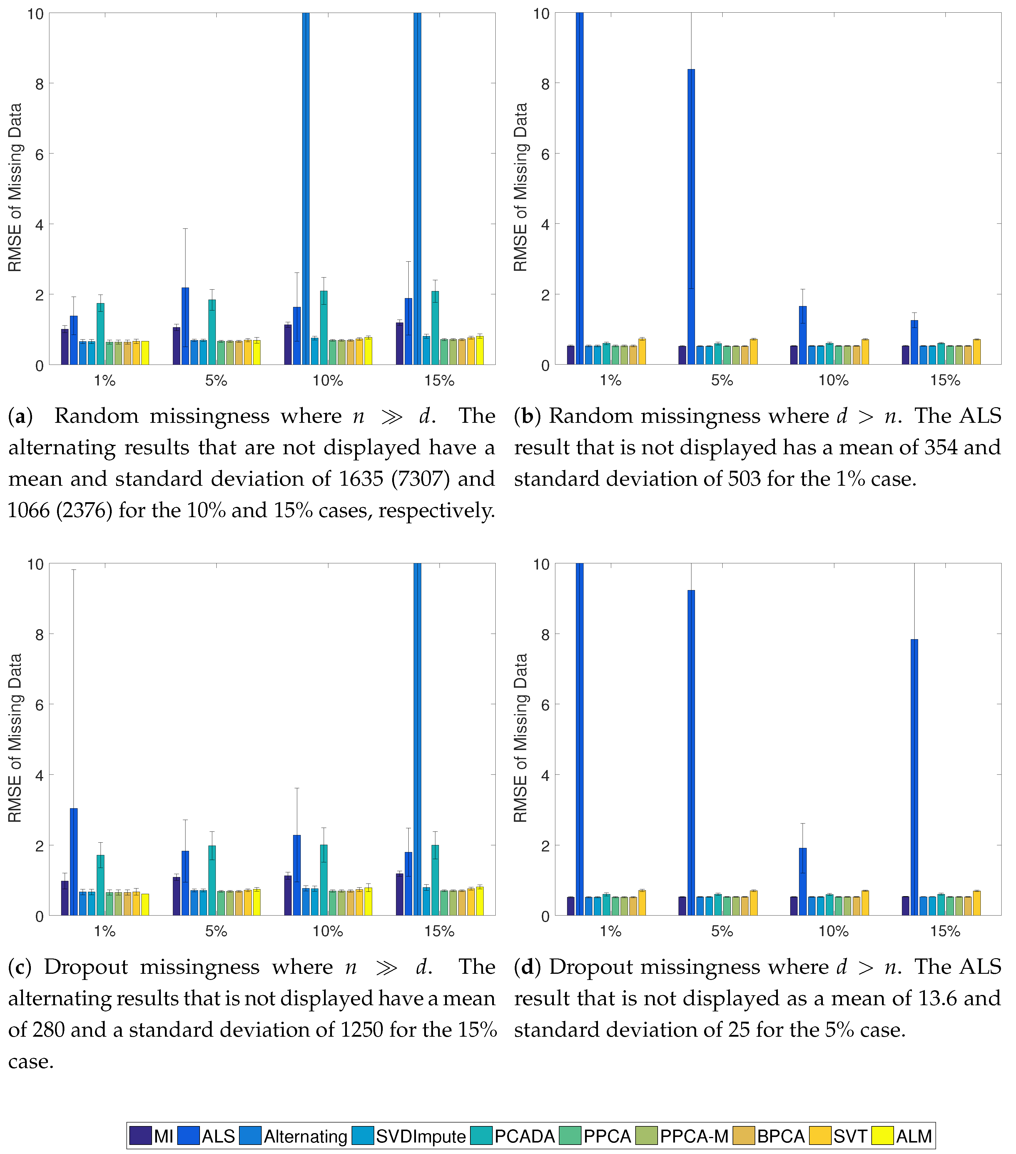
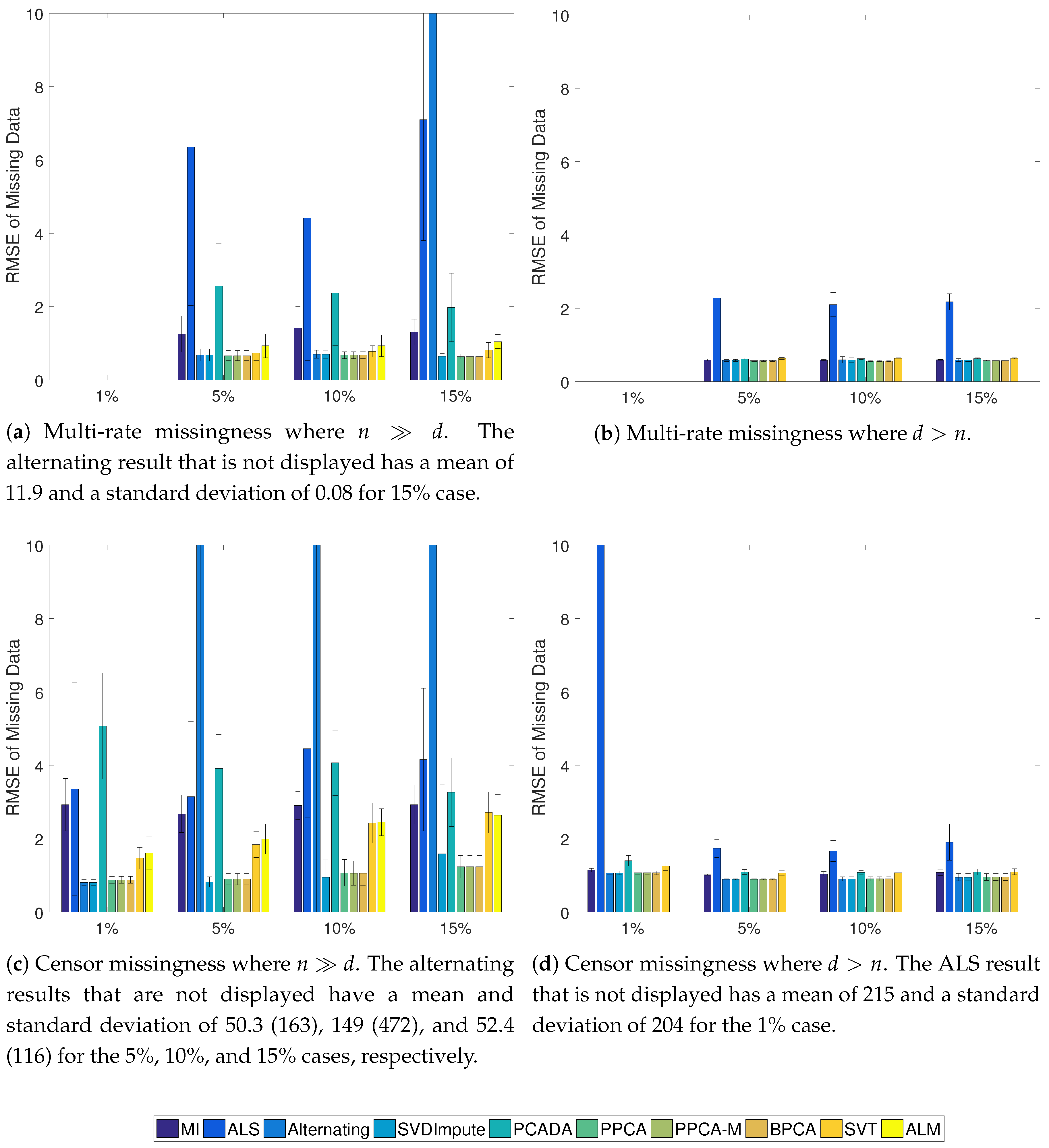
The results of the Gaussian simulations are shown in Figure 2, Figure 3 and Figure 4. SVDImpute and the probabilistic methods (PPCA, PPCA-M, and BPCA) performed the best overall. As the missingness level increased, the probabilistic models performed slightly better, except for SVDImpute performing better for censored data at low levels of missingness. PCADA never outperformed SVDImpute. ALS and the alternating methods both suffered from finding local optima and performed very poorly, as evidenced by the large standard deviations. ALM failed to converge in many cases, and sometimes in all cases, as in the scenarios. The SVT approach fell in the middle while never outperforming the best approaches. For , most approaches did only slightly better than mean imputation whereas significant improvements were observed for , especially in the censoring case.
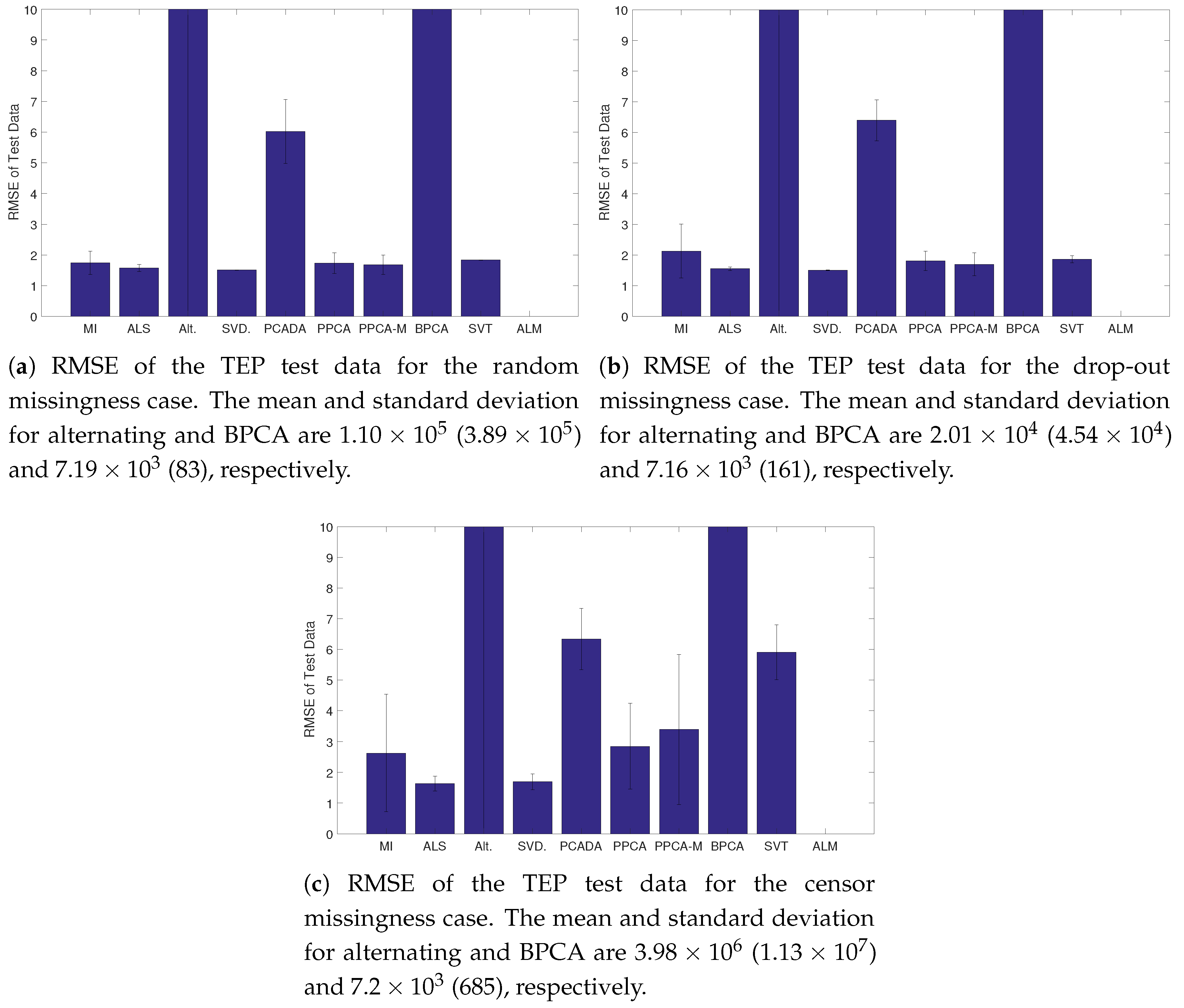
For the TEP, the results of the reconstruction task are shown in Figure 5. For all missingness types, ALS and SVDImpute performed well. ALM failed to converge and Alternating and BPCA had poor results. PPCA, PPCA-M, and SVT performed moderately well, but were more affected by censoring than ALS and SVDImpute. The minimum, average, and maximum number of PCs used in the models, as determined by parallel analysis can be found in Table 1. The number of PCs chosen by SVDImpute, PPCA, and BPCA were very consistent whereas Alternating and PCADA had widely varying number of PCs. Across all methods, the amount of variability in the number of PCs is larger in the censoring case. The results of the fault detection task are in Table 2 and Table 3. For Fault 1, ALS and SVD had the best performance overall, with low detection times and few false detections. MI performed well in terms of detection time but had many false detections. PCADA and BPCA performed the worst overall. For Fault 13, SVT performed the best in the random and drop-out cases, whereas SVDImpute performed the best for the censoring case. PCADA and BPCA again performed the worst overall. ALM was excluded from analysis as no model was learned during the training phase.
4. Discussion
Overall, the best technique to apply PCA in the presence of missing data can depend on the scenario. Several criteria should be considered when choosing an approach, such as the amount of missing data, the missingness mechanism, and the available computational resources. The computational complexity per iteration for each of the algorithms can be found in Table 4, which should only be used as a guideline since the exact implementation will affect computational cost. For instance, SVT [37] and ALM [38] recommend using the Lanczos algorithm to compute the singular values. The Lanczos algorithm is iterative and has reported speed-up of 10× vs. traditional calculation of the full SVD. The Lanczos algorithm returns the singular values that are larger than a certain threshold, which works well in the SVT and ALM frameworks. On the other hand, Lin et al. [38] report that the full SVD computation is faster for scenarios where greater than of singular values are required. While experience indicates that a is significantly lower than d in applications, if no bound on a is known a priori, then the full SVD is typically calculated during procedures to select a, which impacts the computational cost. The probabilistic frameworks have the convenient relation that
which can be used to estimate the percent variance without calculating the full SVD. Another benefit of the probabilistic frameworks is that they are generative and therefore provide parameters for estimation. For all analysis, the test data have been treated as fully observed, which may not be true in practice as new data may be subject to the same type of missingness as the data used in model building. If the data are subject to NMAR missingness, these parameters may not be useful. Note also that the probabilistic approaches can have slow convergence.
The difference in the results of the two ALS approaches also highlights the importance of the exact implementation. Both methods are using the same underlying algorithm but differ in the implementation of the update steps and convergence criteria. Empirically, this results in the Alternating algorithm finding local optima more often as the amount of missing data increases for the case and the ALS algorithm finding local optima more often for .
It may be surprising that the robust PCA methods (SVT and ALM) did not perform better, but it is important to recognize that these methods were developed for cases with very low rank solutions, a large number of missing values, and random missingness. These assumptions are well suited to some applications such as computer vision and imaging but do not necessarily fit the assumptions of missing data in process datasets. A benefit of SVT and ALM is that they can be applied to problems where the location of the corrupt (missing) data is unknown. In the event that additional information is known about the measurement error, methods such as maximum likelihood PCA (MLPCA) [45,46] or heteroscedastic latent variable model (HLV) [47] can be applied to leverage that information. MLPCA is suited to scenarios where the error covariance matrix is known and the errors are correlated or uncorrelated. HLV is suited to scenarios the measurement error is evolving in time. Both algorithms can be applied to scenarios with missing data.
Without additional problem information, we recommend SVDImpute for performing PCA in the presence of missing data for industrial datasets. SVDImpute can be viewed as an implementation of EM [31]. In this view, the missing observations are treated as the unknown variables and , , , and are the model parameters. The corresponding cost function, for only terms involving the parameters, is
where are the imputed values from the SVD. This cost function forces the imputed terms to be near the observed terms which helps to prevent overfitting [31]. A drawback of SVDImpute is that there are many possible reconstructions that will achieve the same result for the observed data, and different results for the missing data, which implies a dependence on the initial guess [31].
In the event that the testing data will also have missing elements, PPCA or PPCA-M is recommended. PPCA-M performs slightly better in the TEP but has higher storage costs during model training. Both result in generative parameters that can be used during the testing phase.
In summary, for missing data problems, the most important step is to determine why some data are missing. If censoring is occurring and not accounted for, the results will be biased. Approaches that incorporate understanding about the underlying mechanisms are likely to perform the best. Expectation maximization frameworks are an important tool in missing data problems and can be applied generally if distributional assumptions are made.
Supplementary Materials
The MATLAB software to add missingness to the datasets can be found at http://web.mit.edu/braatzgroup/links.html.
Acknowledgments
The Edwin R. Gilliland professorship is acknowledged for support.
Author Contributions
K.A.S., M.C.M., and R.D.B. conceived and designed the experiments and wrote the paper. K.A.S. performed the experiments.
Conflicts of Interest
The authors declare no conflict of interest.
Abbreviations
Abbreviations used in this article are:
| ALM | Augmented Lagrange multipliers |
| BPCA | Bayesian PCA |
| EM | Expectation maximization |
| HLV | Heteroscedastic latent variable model |
| MAR | Missing at random |
| MCAR | Missing completely at random |
| MLPCA | Maximum likelihood PCA |
| NMAR | Not missing at random |
| PCA | Principal component analysis |
| PCADA | PCA-data augmentation |
| PPCA | Probabilistic PCA |
| RMSE | Root mean square error |
| SVD | Singular value decomposition |
| SVT | Singular value thresholding |
| TEP | Tennessee Eastman problem |
Appendix A. Definition of the Subspace Angle
To compute the subspace angle between matrices and , where , compute the orthonormal basis of each matrix using the singular value decomposition. Then compute the projection
References
- MacGregor, J.F.; Kourti, T. Statistical process control of multivariate processes. Control Eng. Pract. 1995, 3, 403–414. [Google Scholar] [CrossRef]
- Dunia, R.; Qin, S.J.; Edgar, T.F.; McAvoy, T.J. Identification of faulty sensors using principal component analysis. AIChE J. 1996, 42, 2797–2812. [Google Scholar] [CrossRef]
- Liu, J. On-line soft sensor for polyethylene process with multiple production grades. Control Eng. Pract. 2007, 15, 769–778. [Google Scholar] [CrossRef]
- Kirdar, A.O.; Conner, J.S.; Baclaski, J.; Rathore, A.S. Application of multivariate analysis toward biotech processes: Case study of a cell-culture unit operation. Biotechnol. Prog. 2007, 23, 61–67. [Google Scholar] [CrossRef] [PubMed]
- Yu, H.; MacGregor, J.F. Multivariate image analysis and regression for prediction of coating content and distribution in the production of snack foods. Chemom. Intell. Lab. 2003, 67, 125–144. [Google Scholar] [CrossRef]
- Ku, W.; Storer, R.H.; Georgakis, C. Disturbance detection and isolation by dynamic principal component analysis. Chemom. Intell. Lab. 1995, 30, 179–196. [Google Scholar] [CrossRef]
- Nomikos, P.; MacGregor, J.F. Monitoring batch processes using multiway principal component analysis. AIChE J. 1994, 40, 1361–1375. [Google Scholar] [CrossRef]
- Nomikos, P.; MacGregor, J.F. Multivariate SPC charts for monitoring batch processes. Technometrics 1995, 37, 41–59. [Google Scholar] [CrossRef]
- Imtiaz, S.A.; Shah, S.L. Treatment of missing values in process data analysis. Can. J. Chem. Eng. 2008, 86, 838–858. [Google Scholar] [CrossRef]
- Christoffersson, A. The One Component Model with Incomplete Data. Ph.D. Thesis, Uppsala University, Uppsala, Sweden, 1970. [Google Scholar]
- Wold, S.; Esbensen, K.; Geladi, P. Principal component analysis. Chemom. Intell. Lab. 1987, 3, 37–52. [Google Scholar] [CrossRef]
- Nelson, P.R.C.; Taylor, P.A.; MacGregor, J.F. Missing data methods in PCA and PLS: Score calculations with incomplete observations. Chemom. Intell. Lab. 1996, 35, 45–65. [Google Scholar] [CrossRef]
- Grung, B.; Manne, R. Missing values in principal component analysis. Chemom. Intell. Lab. 1998, 42, 125–139. [Google Scholar] [CrossRef]
- Rubin, D.B. Inference and missing data. Biometrika 1976, 63, 581–592. [Google Scholar] [CrossRef]
- Little, R.J.A.; Rubin, D.B. Statisical Analysis with Missing Data, 2nd ed.; John Wiley & Sons: Hoboken, NJ, USA, 2002. [Google Scholar]
- Qin, S.J. Process data analytics in the era of big data. AIChE J. 2014, 60, 3092–3100. [Google Scholar] [CrossRef]
- Pearson, K. On lines and planes of closest fit to systems of points in space. Lond. Edinb. Dublin Philos. Mag. J. Sci. 1901, 2, 559–572. [Google Scholar] [CrossRef]
- Hotelling, H. Analysis of a complex of statistical variables into principal components. J. Educ. Psychol. 1933, 24, 417–441. [Google Scholar] [CrossRef]
- Jolliffe, I.T. Principal Component Analysis, 2nd ed.; Springer: New York, NY, USA, 2002. [Google Scholar]
- Tipping, M.E.; Bishop, C.M. Probabilistic Principal Component Analysis; Technical Report; Aston University: Birmingham, UK, 1997. [Google Scholar]
- Roweis, S. EM algorithms for PCA and SPCA. In Advances in Neural Information Processing Systems 10; Jordan, M.I., Kearns, M.J., Solla, S.A., Eds.; MIT Press: Cambridge, MA, USA, 1998; pp. 626–632. [Google Scholar]
- Dempster, A.P.; Laird, N.M.; Rubin, D.B. Maximum likelihood from incomplete data via the EM algorithm. J. R. Stat. Soc. Ser. B 1977, 39, 1–38. [Google Scholar]
- Cattell, R.B. The scree test for the number of factors. Multivar. Behav. Res. 1966, 1, 245–276. [Google Scholar] [CrossRef] [PubMed]
- Horn, J.L. A rationale and test for the number of factors in factor analysis. Psychometrika 1965, 30, 179–185. [Google Scholar] [CrossRef] [PubMed]
- Donoho, D.L.; Gavish, M. The Optimal Hard Threshold for Singular Values Is ; Technical Report; Stanford University: Stanford, CA, USA, 2013. [Google Scholar]
- Schafer, J.L. Multiple imputation: A primer. Stat. Methods Med. Res. 1999, 8, 3–15. [Google Scholar] [CrossRef] [PubMed]
- Lee, J.H.; Dorsey, A.W. Monitoring of batch processes through state-space models. AIChE J. 2004, 50, 1198–1210. [Google Scholar] [CrossRef]
- Troyanskaya, O.; Cantor, M.; Sherlock, G.; Brown, P.; Hastie, T.; Tibshirani, R.; Botstein, D.; Altman, R.B. Missing value estimation methods for DNA microarrays. Bioinformatics 2001, 17, 520–525. [Google Scholar] [CrossRef] [PubMed]
- Walczak, B.; Massart, D. Dealing with missing data: Part I. Chemom. Intell. Lab. 2001, 58, 29–42. [Google Scholar] [CrossRef]
- Tipping, M.E.; Bishop, C.M. Probabilistic principal component analysis. J. R. Stat. Soc. Ser. B 1999, 61, 611–622. [Google Scholar] [CrossRef]
- Ilin, A.; Raiko, T. Practical approaches to principal component analysis in the presence of missing values. J. Mach. Learn. Res. 2010, 11, 1957–2000. [Google Scholar]
- Marlin, B.M. Missing Data Problems in Machine Learning. Ph.D. Thesis, University of Toronto, Toronto, ON, Canada, 2008. [Google Scholar]
- Yu, L.; Snapp, R.R.; Ruiz, T.; Radermacher, M. Probabilistic principal component analysis with expectation maximization (PPCA-EM) facilitates volume classification and estimates the missing data. J. Struct. Biol. 2012, 171, 18–30. [Google Scholar] [CrossRef] [PubMed]
- Bishop, C.M. Variational principal components. In Proceedings of the 9th International Conference on Artificial Neural Networks, Edinburgh, UK, 1999; pp. 509–514. [Google Scholar]
- Neal, R.M.; Hinton, G.E. A view of the EM algorithm that justifies incremental, sparse, and other variants. In Learning in Graphical Models; Jordan, M.I., Ed.; Kluwer Academic Publishers: Dordrecht, The Netherlands, 1998; pp. 355–368. [Google Scholar]
- Oba, S.; Sato, M.; Takemasa, I.; Monden, M.; Matsubara, K.; Ishii, S. A Bayesian missing value estimation method for gene expression profile data. Bioinformatics 2003, 19, 2088–2096. [Google Scholar] [CrossRef] [PubMed]
- Cai, J.F.; Candès, E.J.; Shen, Z. A singular value thresholding algorithm for matrix completion. SIAM J. Optim. 2010, 20, 1956–1982. [Google Scholar] [CrossRef]
- Lin, Z.; Liu, R.; Su, Z. Linearized alternating direction method with adaptive penalty for low rank representation. In Advances in Neural Information Processing Systems; Shawe-Taylor, J., Zemel, R.S., Bartlett, P.L., Pereira, F., Weinberger, K.Q., Eds.; MIT Press: Cambridge, MA, USA, 2011; pp. 612–620. [Google Scholar]
- Downs, J.J.; Vogel, E.F. A plant-wide industrial process control problem. Comput. Chem. Eng. 1993, 17, 245–255. [Google Scholar] [CrossRef]
- Russell, E.L.; Chiang, L.H.; Braatz, R.D. Tennessee Eastman Problem Simulation Data. Available online: http://web.mit.edu/braatzgroup/links.html (accessed on 12 April 2017).
- Lyman, P.R.; Georgakis, C. Plant-wide control of the Tennessee Eastman problem. Comput. Chem. Eng. 1995, 19, 321–331. [Google Scholar] [CrossRef]
- Jackson, J.E.; Mudholkar, G.S. Control procedures for residuals associated with principal component analysis. Technometrics 1979, 21, 341–349. [Google Scholar] [CrossRef]
- Kresta, J.V.; MacGregor, J.F.; Marlin, T.E. Multivariate statistical process monitoring of process operating performance. Can. J. Chem. Eng. 1991, 69, 35–47. [Google Scholar] [CrossRef]
- Russell, E.L.; Chiang, L.H.; Braatz, R.D. Data-Driven Methods for Fault Detection and Diagnosis in Chemical Processes; Springer: London, UK, 2000. [Google Scholar]
- Wentzell, P.D.; Andrews, D.T.; Hamilton, D.C.; Faber, K.; Kowalski, B.R. Maximum likelihood principal component analysis. J. Chemom. 1997, 11, 339–366. [Google Scholar] [CrossRef]
- Andrews, D.T.; Wentzell, P.D. Applications of maximum likelihood principal component analysis. Anal. Chim. Acta 1997, 350, 341–352. [Google Scholar] [CrossRef]
- Reis, M.S.; Saraiva, P.M. Heteroscedastic latent variable modelling with applications to multivariate statistical process control. Chemom. Intell. Lab. 2006, 80, 57–66. [Google Scholar] [CrossRef]
- Björck, A.; Golub, G.H. Numerical methods for computing angles between linear subspaces. Math. Comput. 1973, 27, 579–594. [Google Scholar] [CrossRef]
- Wedin, P. On angles between subspaces of a finite dimensional inner product space. In Matrix Pencils; Lecture Notes in Mathematics 973; Kagstrom, B., Ruhe, A., Eds.; Springer: Berlin, Germany, 1983; pp. 263–285. [Google Scholar]
Figure 1.
Possible realizations of the investigated missingness mechanisms: (a) shows random missingness; (b) shows sensor failure which results in missingness that is correlated in time; (c) shows multi-rate data, and (d) shows censored data.
Figure 1.
Possible realizations of the investigated missingness mechanisms: (a) shows random missingness; (b) shows sensor failure which results in missingness that is correlated in time; (c) shows multi-rate data, and (d) shows censored data.
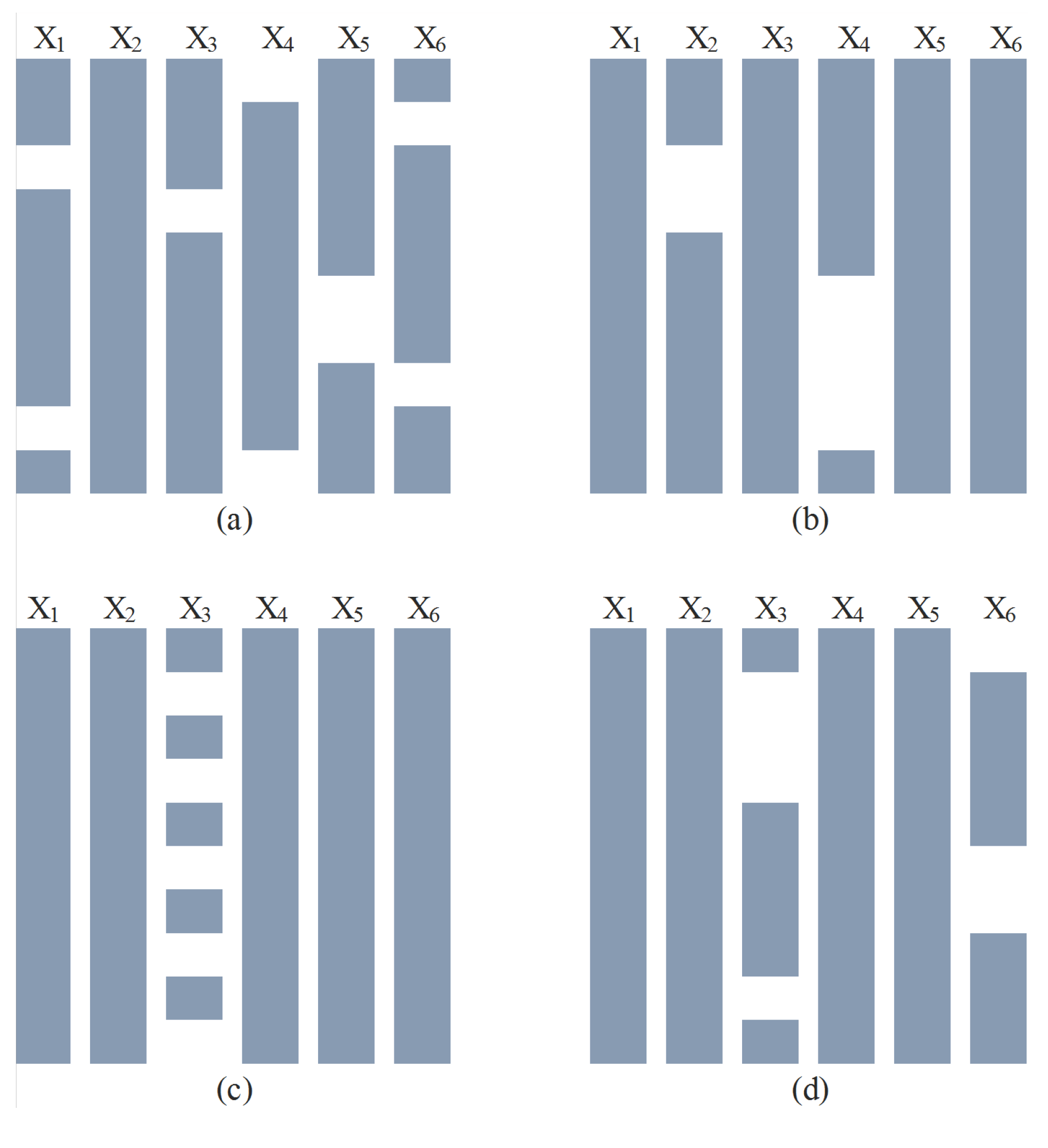
Figure 2.
Average RMSE of the missing data with standard deviation for the Gaussian cases. In the case, ALM never converged to a solution.
Figure 2.
Average RMSE of the missing data with standard deviation for the Gaussian cases. In the case, ALM never converged to a solution.

Figure 3.
Average RMSE of the missing data with standard deviation for the Gaussian cases. In the case, ALM never converged to a solution.
Figure 3.
Average RMSE of the missing data with standard deviation for the Gaussian cases. In the case, ALM never converged to a solution.

Figure 4.
Average subspace angle of learned vs. true subspace with standard deviation for the Gaussian cases.
Figure 4.
Average subspace angle of learned vs. true subspace with standard deviation for the Gaussian cases.
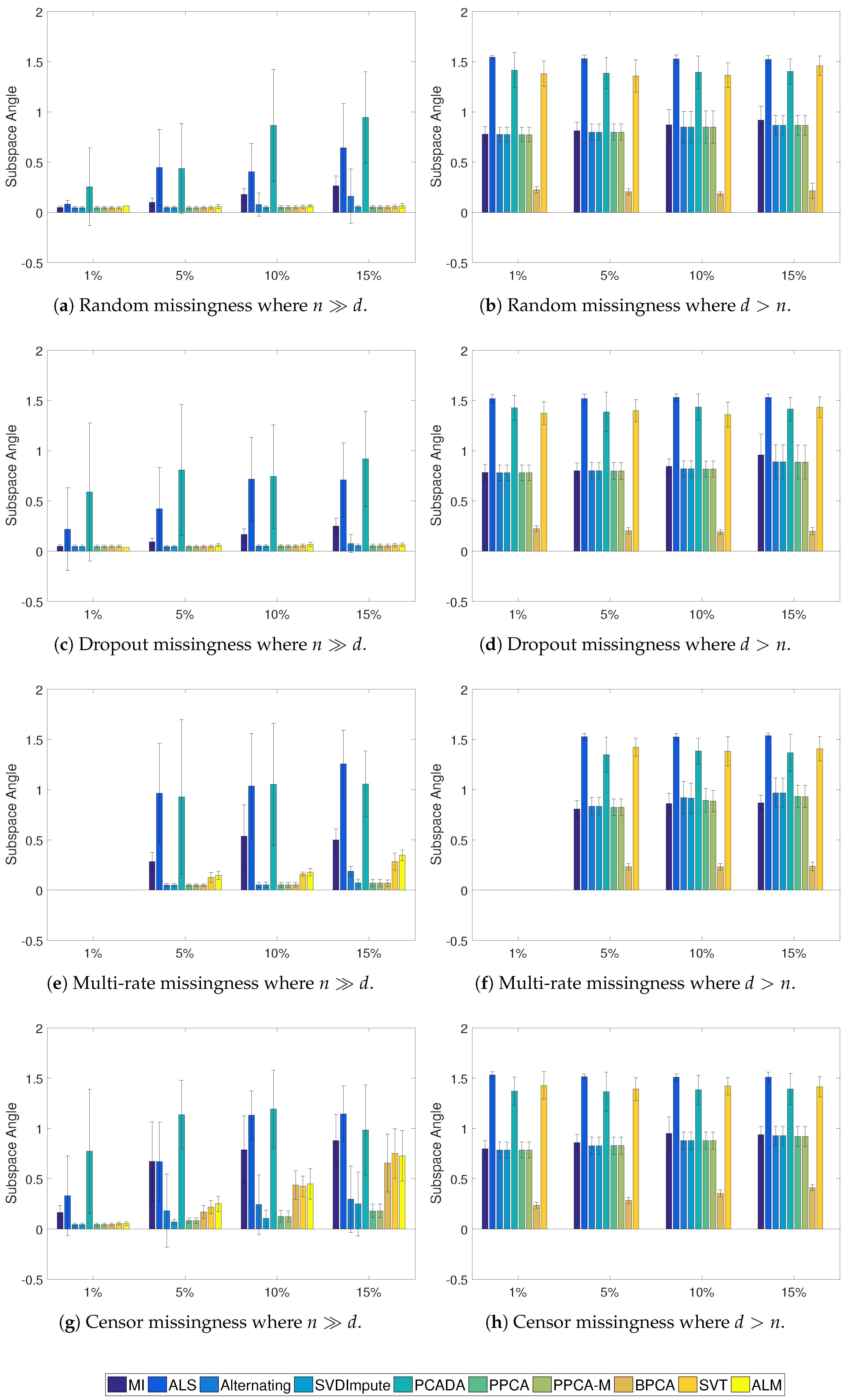
Figure 5.
Average RMSE and standard deviation of the fully observed TEP test set. In all cases ALM failed to converge.
Figure 5.
Average RMSE and standard deviation of the fully observed TEP test set. In all cases ALM failed to converge.


Table 1.
The minimum, average, and maximum number of PCs chosen using parallel analysis for each method over 20 realizations of the missing data. Each missingness type is combined with the naturally arising multi-rate missingness to total 25% missing data. ALM never converged and therefore no results are reported.
| MI | ALS | Alt. | SVD. | PCADA | PPCA | PPCA-M | BPCA | SVT | ALM | |
|---|---|---|---|---|---|---|---|---|---|---|
| Random | ||||||||||
| Min | 2 | 3 | 1 | 3 | 1 | 3 | 4 | 3 | 4 | – |
| Avg | 2.95 | 3.2 | 4.15 | 3 | 2.55 | 3 | 4.3 | 3 | 4.95 | – |
| Max | 3 | 4 | 7 | 3 | 4 | 3 | 5 | 3 | 5 | – |
| Drop | ||||||||||
| Min | 1 | 3 | 1 | 3 | 1 | 3 | 3 | 3 | 4 | – |
| Avg | 3.15 | 3.3 | 4.15 | 3 | 2.65 | 3 | 4.05 | 3 | 4.9 | – |
| Max | 4 | 4 | 6 | 3 | 5 | 3 | 5 | 3 | 5 | – |
| Censoring | ||||||||||
| Min | 1 | 3 | 1 | 2 | 1 | 2 | 1 | 2 | 1 | – |
| Avg | 3 | 3.5 | 3.65 | 2.9 | 2.6 | 2.85 | 3.3 | 2.9 | 1.65 | – |
| Max | 4 | 5 | 7 | 3 | 7 | 3 | 5 | 3 | 4 | – |
Table 2.
The mean detection times for each of the methods and missingness types. Cases are marked by “–” where every trial resulted in a false detection (e.g., a detection prior to ).
Table 2.
The mean detection times for each of the methods and missingness types. Cases are marked by “–” where every trial resulted in a false detection (e.g., a detection prior to ).
| MI | ALS | Alt. | SVD. | PCADA | PPCA | PPCA-M | BPCA | SVT | |
|---|---|---|---|---|---|---|---|---|---|
| Fault 1 | |||||||||
| Random | 163.1 | 163 | 163 | 163 | – | 163.8 | 163.1 | – | 171.0 |
| Drop | 163 | 163 | – | 163 | – | 163.7 | 163.4 | – | 170.5 |
| Censor | 163.1 | 163.2 | 163 | 163.5 | – | 163.2 | 163.4 | – | – |
| Fault 13 | |||||||||
| Random | 182 | 181.8 | 210 | 182 | – | 180.3 | 183.2 | – | 174 |
| Drop | 182 | 181.4 | – | 181.3 | – | 182.3 | 179.3 | – | 174.5 |
| Censor | 180.3 | 181.9 | 411 | 184.9 | – | 185 | 189.7 | – | – |
Table 3.
The number of false detections for each of the methods and missingness types.
| MI | ALS | Alt. | SVD. | PCADA | PPCA | PPCA-M | BPCA | SVT | |
|---|---|---|---|---|---|---|---|---|---|
| Fault 1 | |||||||||
| Random | 0 | 0 | 19 | 0 | 20 | 2 | 0 | 20 | 0 |
| Drop | 9 | 0 | 20 | 0 | 20 | 1 | 1 | 20 | 1 |
| Censor | 5 | 3 | 19 | 3 | 20 | 6 | 9 | 20 | 20 |
| Fault 13 | |||||||||
| Random | 7 | 3 | 19 | 1 | 20 | 4 | 4 | 20 | 0 |
| Drop | 11 | 4 | 20 | 5 | 20 | 5 | 4 | 20 | 0 |
| Censor | 12 | 9 | 19 | 8 | 20 | 19 | 17 | 20 | 20 |
Table 4.
The computational costs of each of the methods where d is the number of measurements, n is the number of samples, a is the latent dimension, and k is the number of bootstrap samples.
Table 4.
The computational costs of each of the methods where d is the number of measurements, n is the number of samples, a is the latent dimension, and k is the number of bootstrap samples.
| ALS/Alternating/PPCA/BPCA | SVDImpute/SVT/ALM | PCADA | PPCA-M |
|---|---|---|---|
© 2017 by the authors. Licensee MDPI, Basel, Switzerland. This article is an open access article distributed under the terms and conditions of the Creative Commons Attribution (CC BY) license (http://creativecommons.org/licenses/by/4.0/).
Share and Cite
MDPI and ACS Style
Severson, K.A.; Molaro, M.C.; Braatz, R.D. Principal Component Analysis of Process Datasets with Missing Values. Processes 2017, 5, 38. https://doi.org/10.3390/pr5030038
AMA Style
Severson KA, Molaro MC, Braatz RD. Principal Component Analysis of Process Datasets with Missing Values. Processes. 2017; 5(3):38. https://doi.org/10.3390/pr5030038
Chicago/Turabian StyleSeverson, Kristen A., Mark C. Molaro, and Richard D. Braatz. 2017. "Principal Component Analysis of Process Datasets with Missing Values" Processes 5, no. 3: 38. https://doi.org/10.3390/pr5030038
Note that from the first issue of 2016, this journal uses article numbers instead of page numbers. See further details here.