Comparison of CO2 Capture Approaches for Fossil-Based Power Generation: Review and Meta-Study


Department of Chemical Engineering, McMaster University, 1280 Main St. W, Hamilton, ON L8S 4L7, Canada
*
Author to whom correspondence should be addressed.
Processes 2017, 5(3), 44; https://doi.org/10.3390/pr5030044
Submission received: 15 June 2017
/
Revised: 19 July 2017
/
Accepted: 28 July 2017
/
Published: 14 August 2017
(This article belongs to the Collection Process System Engineering for More Efficient Power and Chemicals Production)
Abstract
:This work is a meta-study of CO2 capture processes for coal and natural gas power generation, including technologies such as post-combustion solvent-based carbon capture, the integrated gasification combined cycle process, oxyfuel combustion, membrane-based carbon capture processes, and solid oxide fuel cells. A literature survey of recent techno-economic studies was conducted, compiling relevant data on costs, efficiencies, and other performance metrics. The data were then converted in a consistent fashion to a common standard (such as a consistent net power output, country of construction, currency, base year of operation, and captured CO2 pressure) such that a meaningful and direct comparison of technologies can be made. The processes were compared against a standard status quo power plant without carbon capture to compute metrics such as cost of CO2 emissions avoided to identify the most promising designs and technologies to use for CO2 emissions abatement.
1. Introduction
In the US, greenhouse gas (GHG) emissions from electric power generation constitutes about 29% of all GHG emissions over the course of a year [1], mostly arising from the combustion of fossil fuels such as coal and natural gas. However, there are many approaches available for reducing these emissions in meaningful quantities, such as replacing fossil-based power plants with renewable-based plants such as wind, solar, hydroelectric, waste, or biomass-powered electricity generation systems. Other possibilities include focusing on efficiency increases of traditional plants as a way of reducing fuel consumption (and thus GHG emissions across the entire supply chain) for the same power output, or using nuclear-based power generation, which has a very low carbon footprint. Another approach is to continue to use fossil-based power plants, but instead focus on using carbon dioxide capture and sequestration (CCS) as a way of avoiding most of the CO2 emissions while still using fossil fuels. Each of these options has its own strengths and weaknesses in terms of cost, GHG reduction potential, feasibility, geological limitations, socio-political and cultural factors, logistics, resource availability, technical maturity, environmental impacts, and risks. As such, all of these options are likely to continue to play a role in the global electricity generation mix (for a perspective on why and an overview of these technologies for the North American market, see [2]).
This work focuses specifically on CO2 capture technologies and processes. Solvent-based CO2 capture has been in commercial use for decades as a way of either producing CO2 for sale as a chemical or a necessary cleaning step in which CO2 is a contaminant that must be removed, such as in removing the CO2 from raw natural gas, from combustion flue gas, or from synthesis gas in a Fisher-Tropsch process. The basic principle is to contact a gas stream in an absorber with a solvent that is selective for CO2 over the other chemicals in the gas. The CO2-rich solvent can then be regenerated using distillation (usually a stripper-type configuration) to release the CO2 gas from the solvent such that the lean solvent can be reused again. Although the technology itself is reasonably well understood, its application in the power generation sector for the explicit purpose of avoiding GHG emissions for environmental purposes is only in the beginning commercial stages. This is because the amount of carbon dioxide that must be captured from a flue gas is so massive that the sheer size of the project makes it very expensive.
For example, the largest such commercial installment, the SaskPower Boundary Dam Power Station in Saskatchewan, Canada, was completed in 2014. It uses an amine solvent-based post-combustion capture process. From May 2016 to April 2017, the facility averaged about 109 MW of net power output with about 83% uptime and about 58% capture of generated CO2 [3]. This is a significant achievement, especially considering that the captured CO2 is actively being transported via a pipeline and sequestered underground. Some of the captured CO2 is used for enhanced oil recovery, a process in which supercritical CO2 is injected into a spent oil field that enables additional recovery of oil (for a review, see [4]). This is one of the main drivers of the project, because at this location, captured CO2 has value as a product, as opposed to a negative value as a waste. Furthermore, the facility continues to improve its performance and gain valuable experiential knowledge. However, the technology is still not quite mature, since in order to be applied to power plants at the global scale, it must be implemented with a net power output in the 500 to 1000 MW range with CO2 capture rates of up to 90%. It is an open question as to whether 90% is the optimal amount, since there are diminishing returns on increasing this number (the cost and energy penalties per CO2 captured increases as the capture rate increases). However, it is the standard used by most studies and benchmarks, such as by the International Panel on Climate Change reports [5] or the US Department of Energy’s “Baseline” studies [6].
1.1. Post-Combustion Solvent-Based Technologies
A schematic of a supercritical pulverized coal (SCPC) power plant using post-combustion CO2 capture is shown in Figure 1. First, coal is pulverized and combusted with air in a furnace (or boiler). The heat of combustion is used to make steam at various pressure levels, with the highest pressure at about 240 bar (above the critical point of water). The steam produces mechanical power in steam turbines, which are attached by a shaft. The shaft is attached to a generator, which converts the mechanical power to electric power. A condenser is used to produce liquid water from the turbine exhaust, and then a pump is used to recompress the water to supercritical pressures. The combustion exhaust leaving the furnace typically goes through an ash removal, a NOx removal, and a sulfur removal process, in which there are various options for each stage. When CO2 capture is used, the gas leaving the final cleaning stage is sent to a solvent-based CO2 capture process, which removes CO2 for later compression, transport, and storage. The remainder of the gases are exhausted to the atmosphere. Typical solvents for this purpose include monoethanolamine (MEA), diglycolamine (DGA) [7], and methyldiethanolamine (MDEA) possibly mixed with piperazine [8,9].
A typical natural gas combined cycle (NGCC) process with post-combustion CO2 capture is shown in Figure 2. In this process, natural gas is combusted with compressed air at high pressure in a gas combustion turbine, producing mechanical power. Again, a generator is typically attached to convert the mechanical power to electric power. The combustion exhaust leaves at high temperature, and so a heat exchanger network is used to capture this heat by making high-pressure steam for steam turbines, which in turn produce additional electric power. The cooled combustion gases are then subjected to a solvent-based absorption system for CO2 removal. The solvent-based system typically uses an absorber column to scrub the CO2 from the gases, with the cleaned gases exhausted to the flue. The loaded solvent is then purified in a stripper, which recovers lean solvent in the bottom and the CO2 in the distillate for compression and transport.
An alternative to amine-based solvents is ammonia. Although the process is similar in structure to amine-based processes, in the ammonia-based process, aqueous ammonia reacts with CO2 in the flue gas in an absorption tower at atmospheric pressure and low temperatures (either at room temperature [12] or at chilled temperatures of 0–20 °C [13,14]) to form ammonium bicarbonate salts. The flue gas is exhausted after a washing step, and the ammonia bicarbonate slurry leaving the bottom of the absorber is sent to a regenerator at higher temperatures (100 °C) and pressures (20–40 bar) [14] in which the CO2 is desorbed and released as a high pressure gas. The CO2 is washed with water to separate the residual ammonia contained in the gases, and then the CO2 is cooled and compressed to supercritical pressures for pipeline transport. The resulting lean ammonia solution leaving the bottom of the regenerator is recycled to the absorber, and the aqueous ammonia leaving the bottom of the water wash is recovered via a stripper [15].
Alternatively, cryogenic distillation is potentially competitive with solvent-based approaches. In this process, the post-combustion flue gas is first cooled, such that the water is condensed out. Then, the dried flue gas is chilled to between −100 °C [16] and −140 °C [17] depending on the design and the amount of CO2 captured [18]. Under these conditions, the CO2 precipitates out as a solid (for example, on the surface of heat exchangers [19]) thus separating the CO2 from the N2. The CO2 can then be reheated/desublimated to a gas for treatment, compression, and storage. The key weakness is the energy intensity of generating the cooling loads necessary to condense the water and freeze the CO2. Nevertheless, the temperatures are not as cold as the cryogenic air separation [18] necessary for other competing processes (see Section 1.2 and Section 1.3), there are opportunities for heat integration with other processes, and no solvents are necessary. However, because of the lack of techno-economic analysis data available in the literature, cryogenic distillation is not included in the meta-study.
The post-combustion capture approach is attractive in part because it can be retrofitted to existing chemical plants by being “added” at the back end. The ability to use the existing power plant, supporting infrastructure, regulations, contracts, and technical know-how is very beneficial. As such, the cost of a retrofit to an existing plant may be low enough to make sense. However, post-combustion CO2 capture is very expensive and energy intensive. For example, one study found that adding post-combustion solvent-based CO2 capture to a classic pulverized coal power plant caused the average levelized cost of electricity (LCOE) to increase by 50–90% [20]. This means that, although the capture system may recover about 90% of the CO2 actually generated by the facility, the average lifecycle GHG emissions reduction of the plants surveyed in this work is only in the range of 65–71%, which compares well to reported ranges of 50–75% in other studies [21,22,23].
Moreover, because the fuel use is so much higher, adding CO2 capture to a combustion-based power plant makes the environmental impacts as much as 10–67% worse in many other kinds of environmental impact categories [21,22]. For example, one life cycle analysis study concluded that adding post-combustion capture to a coal combustion power plant causes 38% more fossil fuel consumption, 46% more toxicity impacts in humans, 58–59% more toxicity in freshwater, marine, and land-based ecosystems, and 67% more freshwater depletion [22]. The decision as to whether the extra environmental damage in these areas is worth the reduction in climate change potential is at least partially a matter of emotional and political priorities. Life cycle impact assessment methodologies such as the ReCiPe method can be used to help make this comparison quantitatively, but recent studies looking at this issue found opposing results. One group of studies found that post-combustion capture was still better for the environment on the whole despite all of the negative trade-offs for both coal [22] and natural gas [23], while another found that it was better for the environment not to use post-combustion capture at all for either fuel, instead preferring business-as-usual [24]. Nevertheless, Saskatchewan has clearly decided that the trade-offs are worth it, at least for now.
Even so, the significant cost and efficiency penalties of post-combustion capture make it very unattractive for any non-retrofit scenario. For example, if an existing power plant is approaching the end of its lifetime, retrofitting a post-combustion CO2 capture section may not make sense. As the results of this meta-study will show, for new builds, post-combustion capture makes even less sense as a long-term solution. As such, there are a variety of technologies that are currently under development or study that use a completely different approach to generating electricity from fossil fuels specifically to avoid having to use a solvent to recover CO2 from combustion flue gases, and some are not even at the pre-commercial stages yet. These processes include the integrated gasification combined cycle (IGCC), oxyfuel combustion, membrane-based CO2 capture, and solid oxide fuel cell (SOFC) power generation.
1.2. Pre-Combustion Solvent-Based Technologies (Integrated Gasification Combined Cycle)
The next-closest in technical maturity to post-combustion capture is the IGCC process, shown in Figure 3. In this process, a cryogenic air separation plant is used to separate O2 from air. The O2 is fed to a gasifier in which coal is gasified in an oxygen-deficient environment at high pressure (about 50 bar). The oxygen partially combusts some of the coal to produce a mixture of CO, CO2, H2, COS, and H2O (known as syngas) at high temperatures (as high as 1350 °C). This syngas is then shifted using the water gas shift (WGS) reaction, in which the CO and COS are reacted with water to produce H2 and H2S, respectively. Then after a number of cleanup steps, including the removal of water, mercury, and sulfur, the syngas primarily contains just H2 and CO2.
A solvent-based process is used to remove most of the CO2 from this stream for compression and storage purposes, as shown in Figure 4. Both H2S and CO2 need to be removed from the syngas, and the same solvent can be used to remove both. Typically, this is done in two stages, such that the H2S and CO2 can be removed separately using two separate absorbers in series. For the example using Selexol shown in Figure 3, the shifted syngas enters the first absorber, where it contacts a solvent mixture that absorbs the H2S in the syngas (note that this solvent mixture is already loaded with CO2 from the second absorber). The solvent leaving the first absorber (now loaded with both CO2 and H2S) enters a gas stripper, in which some nitrogen is added in order to remove some of the CO2, such that the H2S concentration in the loaded solvent increases. The loaded solvent is then purified in a stripper in which the recovered H2S with some accompanying CO2 is sent to the Claus process for conversion into elemental sulfur. The lean solvent is then used in the second absorber to recover CO2. The larger portion of the loaded solvent leaving the CO2 absorber is regenerated using a series of cascading flash drums (a stripper could be used, but this would be more expensive). Note that the pressure of the recovered CO2 gas from the flash drums is moderately high, such that the costs of CO2 compression are much lower than for SCPC and NGCC post-combustion approaches that capture the CO2 at flue gas pressures (near atmospheric). In addition to Selexol, other suitable solvents for various pre-combustion capture include MDEA [8], MDEA/Piperazine blends [9], MEA [27] (also called EconamineFG [6,28]), diglycolamine [29], and Rectisol [30].
After removal of the CO2, a stream of primarily H2 gas at high pressure remains, which is then combusted in a gas turbine. However, to avoid very high combustion temperatures, nitrogen from the air separation unit is used as a diluent. Like the NGCC case, the exhaust gases from the combustion turbine are sufficiently hot to power a second combined cycle using steam as a working fluid.
One such plant is currently running in Edwardsport, Indiana, USA, though not with the CO2 capture and sequestration component [31]. Another IGCC plant in Kemper County, Mississippi, USA, is still under construction, with $7.3 billion spent as of March 2017 [32], but this includes the CO2 pipeline for transport of captured CO2 (which has already been constructed), and the coal mine as well. IGCC uses a combination of coal gasification and the water gas shift reaction to produce a high-energy stream containing essentially H2 and CO2, such that all of the carbon in the coal ends up in CO2, while most of the energy in the coal ends up in the H2. The CO2 can be separated from the H2 using a solvent-based absorption process, with the remaining H2 combusted in a gas turbine for power. In theory, this pre-combustion solvent-based capture approach carries a lower energy penalty than post-combustion capture, such that the overall GHG emissions and environmental impact is lower than for solvent-based post-combustion capture, although only by about 5–13% [5,22]. Curiously, there is conflicting evidence as to whether IGCC without carbon capture is any better for the environment than current state-of-the-art coal combustion power plants without capture [5,22]. This is also reflected in the survey results of this meta-study, as discussed in Section 3. Noting that the Edwardsport plant was far more expensive than expected [33], this indicates that the primary reason to choose IGCC as far as climate change is concerned is primarily for the slight potential environmental advantage over post-combustion capture when CO2 capture is implemented.
One particular challenge with IGCC is the relatively poor availability of the gasifier, since gasifiers are notoriously difficult to operate. For example, Spliethoff [34] presented the availability of four gasifiers over time (Wabash, Tampa, Puertollano, and Buggenum) and showed that the most successful gasifiers operated at 70–80% uptime, compared to an average uptime for traditional coal and gas combustion of about 88%. The Puertollano gasifier took 5 years after commissioning to reach a peak availability of about 62%, and the Buggenum gasifier took 10 years of gradual improvements to reach 70%. Because of this, it is not uncommon to require the construction of two identical gasifiers, one of which is kept in a hot-standby state to be used in the event of the failure of the other gasifier, such as at the Eastman Chemical Company facility in Kingsport, Tennessee. This allows for an overall 98% system uptime [35], but adds considerably to the cost. If gasifier uptime can be improved significantly, this may help reduce costs and give IGCC a wider acceptance.
An alternative configuration uses an air-blown gasifier instead of high purity oxygen, and uses a pre-combustion capture approach. This simplifies the upstream portions of the process by eliminating the need for high-purity oxygen (thus eliminating the energy-intensive air separation unit). However, because of the large amounts of nitrogen in the syngas, the CO2 capture problem is more difficult, both because of the significantly decreased partial pressure of CO2, and because the CO2 capture problem is a more difficult CO2/N2 separation problem, as opposed to the less difficult CO2/H2 separation problem of oxygen-blown IGCC. This requires an amine (such as MDEA [36,37]). It is also possible to use a post-combustion approach with air-blown IGCC as well, using an amine such as MEA [38] or with chilled-ammonia [39]. However, in both cases, there is little evidence that this would be a substantial improvement (or an improvement at all) over oxygen-blown gasification approaches from a cost perspective. We could not include the air-blown approaches in the meta-study because of the lack of techno-economic data in the literature.
1.3. Post-Combustion Solvent-Free Water Condensation-Based Technologies (Oxyfuels, Solid Oxide Fuel Cells, Chemical Looping Combustion, and Calcium-Oxide Looping).
The key principle of the oxyfuel process is to combust fuels in a N2-lean environment. As shown in Figure 5, cryogenic air separation is used to separate O2 from air, and use the recovered O2 as the oxidant for combustion instead of air. Without N2 present, once the ash, NOx, and sulfur are removed, the combustion flue gases contain primarily a mixture of CO2 and H2O. These are relatively easy to separate via condensation of the water. However, without N2, some other gas must be used as a diluent, and usually captured CO2 downstream is recycled to the combustor for this purpose. Although there are many technical challenges with this approach, pilot plants up to 30 MW have been constructed [40], making them less mature than IGCC, but still feasible for large-scale implementation in the relatively near term. As will be shown in this work, oxyfuels have lower GHG emissions than post-combustion solvent-based capture, and are more cost effective on average, although there is high variability from study to study.
Solid oxide fuel cell (SOFC) power generation systems operate on much the same principle as oxyfuels, in that the fuel should be used without N2 present, such that the exhaust products are an easily-separable CO2 and water mixture. SOFC systems, however, do not use cryogenic air separation, but instead feed ordinary air into the cathode of the SOFCs, as shown in Figure 6. Oxygen in the air, and not nitrogen, migrates through the solid barrier to the anode, where it reacts electrochemically with the fuel. As such, the SOFC acts as both electric power generator and air separator. It is a high-temperature (>800 °C) process with its own set of technical challenges, with low cell lifetime and difficulty of manufacture being just two of the major barriers to commercialization [42]. SOFCs are commercially available up to the 250 kW scale, but are largely used in niche markets, such as low-noise and low-vibration applications. As such, they are less mature than oxyfuels, but it is still within the realm of technical possibility to design large-scale processes which use existing materials and designs. However, much like IGCC and oxyfuels, various studies suggest that unless SOFC costs can be reduced significantly, SOFC power plants are not likely to be economically competitive with traditional power plants on a purely cost basis. Instead, their primary attractiveness is that SOFC systems combined with CCS tend to be better than post-combustion solvent-based alternatives in terms of cost, GHG reduction potential [22,42,43,44], or the balance between the two, as will be shown in Section 3.
Like oxyfuels and SOFCs, chemical looping combustion (CLC) processes are designed to combust fuel without the presence of nitrogen by using a metal as an oxygen carrier. With this approach, oxygen is removed from air by reacting air at high pressure with reduced metal particles (such as nickel, iron, or calcium), thus producing a hot stream of metal-oxide particles entrained in hot air. The metal oxide particles are separated from the spent air via cyclone, and the cleaned, hot, high-pressure air is fed to a turbine to recover electricity. The recovered hot metal oxide particles are then reacted directly with a gaseous fuel (also at high pressure, such as syngas, natural gas, or hydrogen). The fuel is oxidized into CO2 and H2O, still at high pressure, by reducing the metal oxides. Heat is recovered from the CO2/H2O stream for steam generation for additional power, and the CO2 can be captured by condensation of the water. The reduced metal is then returned to the air reactor, where it is oxidized again, thus completing the loop. A summary is shown in Figure 7. For extensive reviews on this topic, including how this process can be modified for the purposes of coal gasification or hydrogen generation, see [45,46].
Calcium looping processes (CLP) take a different approach to CO2 capture in which CO2 is directly reacted with calcium oxide [47,48,49] or calcium hydroxide [50] to produce solid calcium carbonate, which can be separated easily from flue gas. The calcium oxide is regenerated in a calcination reactor by reaction with high-purity oxygen and recycled for more CO2 capture. The calcination reactor is highly endothermic, and requires a large heat supply at high temperatures (above 800 °C), which is often met by in-situ oxy-combustion of coal or natural gas inside the calcination reactor. The CO2 released from the calcination reactor is captured and compressed for storage after a heat recovery step. A spent sorbent purge stream is removed from the calcination reactor, in part because of the build-up of calcium sulfate and other solids that result from reactions with impurities in coal or other fuels. The key advantage is that there are many opportunities for heat integration within this process and with other processes. The key disadvantages are the large parasitic load of producing high purity oxygen, the relatively large amount of make-up sorbent (calcium carbonate) required, and the somewhat low CO2 capture rate (around 85%). An example process is shown in Figure 8.
1.4. Pre-Combustion and Post-Combustion Membrane-Based Technologies
Membrane-based approaches use a variety of techniques that can be classified as either pre-combustion or post-combustion. Pre-combustion membranes use a gasification approach similar to IGCC, in which gasification and water gas shift reactors are used to produce a mixture of CO2 and H2, with a membrane (or multiple stages of them) used to separate CO2 from H2 instead of a solvent-based process. Either the CO2 or the H2 could be the permeating species, depending on the design of the system. An example superstructure of the processes surveyed in this meta-study is shown in Figure 9. In this case, the upstream portions of the process are very similar to the upstream portions of the IGCC process (Figure 3) or the coal-based SOFC process (Figure 6), in which desulfurized, shifted syngas is produced (primarily consisting of H2 and CO2). An H2/CO2 selective membrane is used to separate this into the component streams, with the captured CO2 sent to a compression train for sequestration, and the remaining H2 (with some CO2 remaining) used for combustion in a gas turbine. It may also be possible to enhance the H2/CO2 membrane separation performance by using a membrane-enhanced water gas shift reactor, in which some of the H2 is removed in the water gas shift reactor itself, as the reaction occurs. This has the dual benefit of shifting the reaction equilibrium toward a higher CO conversion (either resulting in more H2 and CO2 production or permitting operation at higher temperatures) and increasing the CO2 concentration of the reactor effluent by removing the H2 product. Nitrogen can be used as a sweep gas on the permeate side of the membrane-enhanced water gas shift reactor since the hydrogen gas needs to be diluted with nitrogen anyway before combustion in the gas turbine to prevent extremely high temperatures.
Alternatively, post-combustion membranes are used to remove CO2 from combustion flue gases instead of post-combustion solvent-based capture. They may also be used to enhance solvent-based systems as well. A superstructure of common designs surveyed in this study is shown in Figure 10. Typically, the dewatered combustion flue gases (containing primarily N2 and CO2) are compressed from near-atmospheric pressure to a high pressure and sent to a membrane for CO2/N2 separation, which may or may not use a sweep gas in the permeate side. A vacuum is drawn on the permeate side to recover CO2 at low pressure, and so this gas must be recompressed back up to high pressure again. Depending on the nitrogen content and process design, the permeate can either be sent to a second stage membrane for additional CO2 purification (called Route 1 in Figure 10) or sent directly to CO2 liquefaction (Route 2). In Route 2, an optional membrane could be used to partially separate the gases remaining from CO2 liquefaction, with appropriate recycles. Additionally, it may be desirable to use an additional membrane to remove additional CO2 from the retentate of the first stage membrane (Route 2) using boiler feed air as a sweep gas. This will remove additional CO2 and increase the CO2 content of the flue gas, resulting in a potentially greater CO2 recovery rate and potentially better separation in the first stage membrane due to higher CO2 concentrations. Although post-combustion membrane systems avoid solvent-based separation, one key disadvantage of these systems is the large compression load due to large pressure drops across the membranes.
Lastly, with the wide variety of process approaches and differences in implementation for all of the above technologies, it is difficult to gauge which technologies we should be pursuing now and in the future from the existing literature. Although many techno-economic studies of CO2 capture processes often make comparisons with some base case to determine metrics such as LCOE or CO2 emissions avoided, nearly all studies use different fuel costs, cost methods, base cases, and other assumptions which make a direct cross comparison of one study to another rather difficult. It is therefore the goal of this meta-study to examine a broad range of studies and processes in the literature and make informed comparisons between them using consistent metrics. Such a study has not been presented before in the literature to the best of our knowledge. For example, [5] has an excellent comparison of the CO2 emissions of traditional post-combustion, IGCC, and oxyfuel plants, but it does not include SOFC or membrane technologies, nor does it have any indication of costs either. The present study, however, includes these technologies and not only examines life cycle CO2 emissions, but the relative costs of avoiding them using a consistent basis for all technologies.
2. Research Methods
In this work, we surveyed and examined techno-economic studies of power plant systems with CO2 capture capabilities published since 2007 (for a review of CO2 capture technologies prior to 2007, see [12,51]). The following CO2 capture strategies were considered to be classified by these types: traditional combustion with solvent-based post-combustion CO2 capture, IGCC with pre-combustion CO2 capture, oxyfuels, membrane-based processes, and solid oxide fuel cells. Since none of these technologies has been fully commercialized, all of these studies are theoretical in nature, and are typically based on first-principles chemical process modelling and simulation. Although each study considered provided some information concerning basic economic and performance metrics (costs, efficiencies, CO2 capture rates, etc.), the assumptions and methodologies used to compute these metrics differ from study to study. Moreover, the processes’ objectives varied from study to study, such as the total power produced, the amount of CO2 captured, and the quality and pressure of the captured CO2. Therefore, in this work, we used a normalization strategy in order to predict the costs and performance of each process using a consistent basis of comparison.
2.1. The Standard “Status Quo” Plant
In this work, we use a single “status quo” plant design for the base case for comparison in the coal and natural gas categories. In the coal category, the base case plant is a supercritical pulverized coal power plant without CO2 capture. For natural gas, the base case used is a natural gas combined cycle power plant. Both adequately represent commercially mature conventional power plant designs in use today. All studies assume baseline-only operation. The key characteristics for these plants are shown in Table 1. These plants were chosen as the basis of comparison because of its clarity of methods, availability of details, consistency in net power output at a reasonable scale (550 MW), as well as using a consistent approach for comparing both coal and gas fuels in the modern US market. Costs were converted to $US2016 using the methods described later in this section.
2.2. Adjusting for Scale
All plants surveyed were converted to have the same net power output as the base cases shown in Table 1 (550 MW). The non-fuel portion of the costs primarily consist of capital costs, but also consist of other factors such as maintenance and overhead, labour, spare parts, working capital, and accounts receivables [53]. It is typical to estimate the costs of these other factors as percentages of the total equipment cost [54], and as such, they are all relatively proportional to each other. Because it is a power plant, raw material costs are insignificant compared to the capital or fuel costs. Therefore, a power law adjustment rule (commonly known as the “six-tenths rule”) was used to estimate the costs of the non-fuel portion at the new scale according to the following formula:
where , is the cost of the non-fuel portion at the standard size shown in Table 1, is the cost of the non-fuel portion as reported in the original work (in the given currency per MWh of net power produced), and are the net power output at the standard size and as reported in the original work (in MW), respectively, and is the power law exponent. Commonly, is assumed (hence “six-tenths” rule) when there is a lack of information about the economies of scale for a particular application [54], which derives from historical data for the industry in general. However, in this work, we have adopted as our base case assumed value, based on the studies of Hamelinck et al. [55], which estimated for a wide variety of chemical process equipment relevant to energy and electricity production to be in the range of 0.6 to 1.0, with a tendency on the higher side. For example, they suggested for gasifiers, Selexol-based pre-combustion CO2 capture systems, heat recovery and steam generators, gas turbines, and combined cycled power plants. Larger was recommended for other relevant process operations such as solids handling systems (e.g., conveyors, dryers, and solid feeding systems), as well as air separation, oxygen compression systems, and dry gas cleaning. Moreover, when a plant is “scaled up” by a large amount, the sensitivity of key metrics like levelized costs of electricity (LCOE) to is not insignificant. Therefore, we have conducted a sensitivity analysis on this assumption, as described in Section 3.4, but noting that the final conclusions were essentially unchanged with regard to .
We assume that the efficiency of a given power plant is the same at the standard size as it is at the size of the plant originally reported, since all plants surveyed were within the same order of magnitude (approximately 200 to 1000 MW net power output). As such, the amount of fuel used scales linearly with size, and the amount of fuel required per MWh of electricity produced does not change with size. Expressed in equation form, this becomes simply:
where and are the costs of fuel in the given currency per MWh of net power produced at the standard size and at the size of the plant as originally reported, respectively.
For some studies, the fuel and non-fuel costs were not itemized or reported separately, but either the total costs or the LCOE were reported. In these cases, the fuel costs and non-fuel costs could be approximated using the reported efficiency of the power plant and the unit price of fuel. For example, for a case where the efficiency of the plant, LCOE, and fuel prices were reported, the fuel and non-fuel costs could be computed as follows:
where is the reported electrical efficiency (HHV), is the unit price of fuel as reported (in the reported currency per HHV of fuel in MJ), and is the levelized cost of electricity reported for the original plant (in the reported currency per MWh of net power output). Note that the term in parenthesis in Equation (3) is commonly known as the heat rate, which is sometimes reported directly. In some cases, the reported efficiency was given in lower heating value (LHV) and so was converted to HHV for this purpose.
It is also important to note that LCOE definitions may vary from study to study, such as in using different assumed capacity factors, plant lifetimes, discount interest rates, or whether a constant-dollar or current-dollar approach was used. In most of the works included in the meta-study, these parameters were not provided and only LCOE was reported directly. Since there was insufficient data to convert reported LCOE forms to a standard LCOE form using a standard set of parameters, and the fact that the change in the values would be small anyway, we have taken all reported LCOE numbers at face value, assuming that the authors used reasonable values for these parameters.
Studies which did not have sufficient information to estimate both the fuel and non-fuel cost according to the above procedure were not included in this meta-study.
2.3. Adjusting for Currency Type, Location, and Year
The studies surveyed were conducted using different currency types, countries of construction, and currency years. Reported costs in the literature were converted as follows. First, when non-fuel costs were reported for locales outside the United States, the historical Purchasing Power Parity Index (PPPI) [56] was used to estimate the costs of an equivalent plant if it were located in the United States, instead. This includes both the currency exchange rates as well as relative differences in costs of materials, products, and services. Then, the non-fuel costs were scaled to $US2016 by using the IHS North American Power Capital Costs Index, which is a quarterly capital cost index for the construction of new power plants within North America [57]. The resulting equation is as follows:
where is the nonfuel cost in $US2016 per MWh of electricity produced, is the Power Capital Costs Index of either the first quarter of 2016 or the average index for the year of the original study, and is the Purchasing Power Parity Index for the country of original work for the year of the original study with units of the local currency per $US in the year of the original study. Note that studies that used a United States local use the PPPI for the United States, which is equal to 1 $US/$US by definition.
A similar approach was used for fuel costs, except that instead of using PPPI to convert prices to a US locale, a more specific energy index was used instead. This is because the PPPI and relative energy prices are often vastly different, despite the fact that energy prices do influence the PPPI to some degree. For example, the price of imported natural gas in Germany in 2012 (when converted to US Dollars) was nearly four times the US Henry Hub price [30], but the relative price of goods in general using the PPPI between Germany and the US in 2012 was very close to 1 [56]. When the fuel costs or unit price of fuel was provided in the original study, it was first localized to the United States in $US in the base year using relative pricing information published by BP [58] and the currency exchange rate [59], and then scaled to the current year by using the ratio of the historical fuel price index for North America based on price history data from the US Energy Information Administration [60]. The equation is as follows:
where is the fuel cost at the standard size (in $US2016 per MWh of net electricity produced), is the historical currency average exchange rate for the project year of the original study in $US per local currency unit, is the relative price ratio of fuel (the average price of coal or gas in the US divided by the price of the same amount of fuel in the country of the study in the $US for the year of that study), and is the energy cost index for either bituminous coal or conventional pipeline natural gas for the North American market, for either the first quarter of 2016, or the average of the base year. In some cases, the project year of the study was not reported, and so the year of publication of the study was used as an approximation instead. The LCOE of each plant for the standard size and year () in units of $2016 per MWh of net electricity produced becomes:
Note that the LCOE computed does not consider distribution costs, profits/markups, or taxes.
In addition, we considered a second set of assumptions, in which the unit price of fuel for 1Q2016 in the North American market was used directly [60] and the originally reported fuel price was ignored. The reason for this was that fuel is a global commodity with readily tracked and recorded prices based on specific markets, and it would make sense to use the same price of fuel for each case when comparing many different kinds of power plants to each other on the most consistent basis possible, including the geographical location of construction. In some studies, the assumed fuel prices were far from both known historical market prices for their respective markets, and far from the assumptions made by other researchers (see the Section 3.2 discussion on outliers), and thus were not necessarily good values to include in the meta-analysis.
However, it is also the case that most techno-economic analysis studies are performed with some sort of optimization approach (even informally), in which the trade-offs between the fuel and non-fuel costs are balanced based on an economic objective function. For example, in cases where fuel prices were assumed to be high, researchers would be more likely to make design decisions that favour more expensive but more fuel-efficient designs, and vice versa. Therefore, the non-fuel portion of the costs as calculated in each study are in fact very likely related to the assumed fuel price. Therefore, it is not clear if the fuel prices used in the meta-analysis should be all the same in order to have a constant basis for comparison, or, based on the originally assumed prices in the cited studies in order to preserve the fuel vs. non-fuel trade-offs that factored into design decisions. Thus, both approaches were used in order to draw more general conclusions, and to serve as a sensitivity analysis on fuel price. Lastly, in a few cases, there was not enough information provided in a study to infer fuel price assumptions, and as such only the standard 1Q2016 North American energy price approach could be used.
2.4. Adjusting for Differences in CO2 Capture Rates, Pressures, and Plant Gate Definitions
For this study, we defined the “plant gate exit” to include the compression of captured CO2 up to at least 115 bar pressure, and its purification to minimum pipeline purity standards (at least 95 mol % pure CO2 [61]). All of the studies included in the meta-analysis fell into this standard, although in some cases, the specific pressure was not reported but it was noted that the outlet pressure did meet non-specific pipeline specifications (which are typically at 115 bar or above). The CO2 pressure of the studies surveyed ranged from 115 to 154 bar. Because CO2 is supercritical in that pressure range, pressure increases from 115 up to 154 bar can be achieved using a pump, which is relatively inexpensive compared to the costs of a compressor. For example, the energy required to compress and pump CO2 from 18.5 bar to 115 bar is over 16 times the energy requirement of pumping supercritical CO2 from 115 to 154 bar [25]. Therefore, differences between processes due to differences in CO2 compression pressure were neglected (since all studies cited considered capturing CO2 at pipeline pressure) because the impact on the LCOE is negligible.
The percentage of CO2 captured varies in each plant in the study. Typically, between 90 and 95 percent CO2 created by fuel oxidation was captured for the solvent-based and membrane-based designs. The oxyfuel and SOFC designs typically had CO2 capture rates approaching 100%. Because these differences in capture rates are case-specific and typically linked to a particular design or technology, we did not attempt to alter the cost estimates for each plant to meet a particular CO2 capture percentage.
For standard comparison in this study, the LCOE used for cost comparisons do not include CO2 transport and storage, since those are likely to depend heavily on geography and end-use. All studies considered in this work use reported costs that do not consider transportation and storage. In some cases, this required manual recalculation of either LCOE and/or non-fuel costs to make this adjustment.
2.5. Computing Costs of CO2 Avoided
The total cradle-to-plant-exit lifecycle greenhouse gas emissions were computed as the sum of the direct emissions of the plant itself plus the indirect emissions associated with the production and delivery of the fuel. The total direct emissions of the plant itself were usually reported in each study surveyed in terms of global warming potential in units of CO2 equivalents (CO2e). However, because these studies are simulation based, other greenhouse gases such as NOx are either ignored or are present in very small quantities, such that the total direct emissions of CO2 (the chemical) is essentially equal to the total global warming potential in terms of CO2e.
For studies in which the direct CO2 emissions were not reported, they were estimated by using other information available. For example, given a known CO2 capture percentage and a known efficiency, the CO2 emissions rate could be computed by assuming that all fuel is completely oxidized such that all carbon atoms leave as CO2. For some studies, the direct emissions were not reported in terms of CO2e, but rather the emissions of the individual species of chemicals were reported instead. In this case, this information was used to compute the total global warming potential using the International Panel on Climate Change 5th Assessment 100-year metric (i.e., 1 kg of N2O emissions = 298 kg of CO2e) [62]. In some cases, CO2 emissions were reported, but the effects of NOx were not considered, resulting in an underestimate of the total global warming potential. In these cases, the NOx emissions were estimated by assuming 0.318 kg NOx/MWh produced for SCPC plants and 0.18 kg/MWh and IGCC plants [63]. For calcium looping studies, these numbers are applied to the upstream portions of the power plant (either SCPC or IGCC) only; it is assumed that no NOx is produced in the calciner because of the very small presence of N2.
The indirect emissions associated with the cradle-to-plant-entrance production and delivery of coal was 30.8 kg CO2e per MWh of coal delivered [64]. This number includes the emissions associated with mining and transporting bituminous coal 100 km to the plant entrance. Interestingly, almost two-thirds of the greenhouse gas potential is due to methane emissions (such as from fugitive coal-bed methane), not CO2 itself [22]. Similarly, the indirect emissions for natural gas was 32.8 kgCO2e per MWh of gas delivered [65] by assuming conventional pipeline gas made from the North American average mixture of gas sources (conventional, associated gas, coal bed methane, shale gas, tight gas, off-shore gas, and imported liquefied natural gas). The indirect emissions of electricity transportation (e.g., high-tension transmission lines) or CO2 transport and storage were not included, as they are downstream of the plant in question and are specific to each unique implementation. Emissions associated with the construction of the power plants themselves were neglected, as prior studies found that the construction contributions for SCPC, IGCC, and SOFC-based plants were a very small percentage of the total emissions [22,23].
The cost of CO2 avoided (CCA) is a useful metric for comparing unlike processes in terms of finding which process is the most effective way to spend money for the explicit purposes of reducing CO2 emissions. The CCA is generally defined in reference to a base case plant used as the status quo or business-as-usual case, and is essentially the extra costs that one spends on a process or activity for the specific purposes of avoiding CO2 emissions caused by the base case divided by the amount of CO2 emissions you avoid as a result. This results in the following equation:
where and are the LCOE (in $US2016 per MWh) and cradle-to-plant-exit global warming potential (in tCO2e per MWh of net power output) of the base case (in Table 1), and is the cradle-to-plant-exit global warming potential (in tCO2e per MWh of net power output) of the plant. In this study, we have chosen to use two base cases, one for coal, and one for gas. As such, we report two CCAs, each in relation to the SCPC case (without CO2 capture) or the NGCC base case (without CO2 capture) in Table 1. Note that Table 1 also contains a calculation of the CCA when building the NGCC base case (without CO2 capture) instead of the SCPC base case. This value is negative, meaning that NGCC has both a lower LCOE than SCPC and lower lifecycle CO2 emissions than SCPC. In other words, with current fuel prices and construction costs, there is little incentive to choose an SCPC plant over an NGCC plant from either an economic or an environmental perspective.
The above CCA definition does not determine the CCA of retrofitting a CO2 capture system onto an existing power plant. It also does not compare the CCA by building a power plant of an advanced technology such as SOFCs with CO2 capture compared to the advanced technology without CO2 capture. This is important to note because many studies present CCA numbers using the latter definition. Although that definition of CCA is interesting for that specific study, it cannot be used for cross-comparison across studies.
Lastly, it is important to note that although CCA is a useful metric for understanding the cost trade-offs in terms of a reduction in the global warming potential, it does not consider any other environmental effects such as acid rain, eutrophication, smog, ozone depletion, etc., and so it is not a substitute for a holistic picture of environmental impact. However, the CCA metric is immediately relevant to policy decisions with regard to carbon management and carbon taxes.
3. Results
3.1. Raw Data
The coal cases are summarized in Table 2. The table includes a classification of the process into one of five categories (SCPC, IGCC, COXY = coal-based oxyfuel combustion, IGFC = integrated gasification solid oxide fuel cell, and CMEM = coal-based membrane approaches), with the primary CO2 capture approach described briefly. The base year is the project year as reported in the study. The LCOE is given both as reported and as converted to the standard plant conditions by the methods described in Section 2. The CCA is given using both SCPC and NGCC baselines (in Table 1) as the base plant for comparison, at the standard plant conditions as calculated according to the methods of Section 2. The lifecycle CO2 emissions are for the cradle-to-plant-exit and calculated as described in Section 2.
The natural gas cases are summarized in Table 3. The four categories included were NGCC, NOXY = natural gas based oxyfuels, NMEM = natural gas based membranes, and NGFC = natural gas solid oxide fuel cells. There were far fewer cases for natural gas available in the recent literature that contained the necessary information required for the meta-study. This is primarily because most studies on CO2 capture focus on coal since it has a much larger CO2 intensity compared to gas, and there is less incentive to use CO2 capture in natural gas power plants. For example, in the United States, federal limits on the CO2 emissions of new power plants were set by the US Environmental Protection Agency in 2015 at 1400 lb CO2e per MWh for SCPC (635 kg CO2e/MWh) and 1000 lb CO2e per MWh for NGCC (454 kg CO2e/MWh) [106], which is specifically chosen such that coal-based power plants would require CO2 capture, but state-of-the-art natural gas plants would not. It is possible that these standards for new plants will be modified or removed under the new administration, since the rule is now under official review [107], and the proposed rule for existing plants (which was never formally adopted) has been officially dropped [108]. In addition, a recent set of studies of cradle-to-grave life cycle impacts for coal and natural gas combustion plants with post-combustion capture showed that while adding CO2 capture to a SCPC plant reduces cradle-to-grave lifecycle CO2 emissions by about 74%, adding CO2 capture to an NGCC plant reduces them by only about 67% [22,23].
3.2. Identifying Outliers
Due to the broad nature of assumptions and methodologies used in the studies surveyed, it is necessary to identify outliers that may result in potentially incorrect conclusions. Some can be identified visually. Figure 11 shows a plot of the unit fuel prices and non-fuel costs for coal-based power plants as reported by each study, scaled to the standard conditions according to the methods of Section 2. The dashed rectangle is the visually identified region of the set of normal results, with the points lying outside classified as outliers. Note that no formal method was used to identify outliers, except that these points had unit fuel prices more than ±35% from the mean fuel unit price of $1.97/GJ $US2016 (note the average 2016 coal price was very close at $2.01/GJ [60]).
The three points on the low end are COXY-9, COXY-15 and COXY-16. However, out of these, only COXY-9 appears to be an outlier in terms of both low non-fuel costs and low assumed fuel prices. COXY-12 and COXY-13 have average assumptions for fuel price, but have unusually high non-fuel costs. This is because COXY-12 and COXY-13 use additional purification steps in order to achieve much higher than normal CO2 purities (about 99%) than in most CO2 capture applications (specifically double-flash purification for COXY-12 and direct distillation for COXY-13). Therefore, they are outliers because their design objectives are significantly more stringent than the other selected studies, and so it is not fair to compare them with the other studies directly. CMEM-6 through CMEM-9 are outliers in both non-fuel (disproportionally low) and fuel (disproportionally high), but they were not removed from the analysis because their key metrics, such as LCOE and CCA, were comparable with other coal-based membrane studies.
In general, however, there is surprisingly little correlation between calculated non-fuel costs and classification of power plant. The membrane, oxyfuels, IGCC, SCPC, calcium looping, and chemical looping combustion classes span most of the entire range of the data set, with oxyfuels having the widest range. The SOFC non-fuel costs are consistently on the low-end as predicted by reasonable diversity of authorship (four different groups). However, note that SOFCs still remain unproven for CCS systems or at the 500 MW scale without CCS.
Natural gas outliers could not be identified, since the number of data points was low.
3.3. Trends in Key Metrics
Figure 12 shows the standardized LCOE of each plant using the as-reported fuel prices versus the life cycle CO2 emissions (from the cradle to the plant exit). Some very clear trends emerge. First, the NG-based SOFC systems are clearly the best in terms of both LCOE and GHG emissions, with coal-based SOFCs coming in at a close second. Both classifications are also clearly outside the ranges of competing strategies such as NGCC and oxyfuels of either type, indicating a distinct difference due to the difference in technology paradigm. There is also sufficient agreement among the different independent research groups studying SOFC systems, such that, even if the SOFC studies that were published by members of our own research group were removed (for the sake of eliminating bias), the results remain essentially unchanged. The NGCC systems with CO2 capture have a wider range in LCOE (with the most expensive being almost double the least expensive), but are very close in agreement on lifecycle GHG emissions. Generally speaking, the NGCC systems with CCS are preferable to oxyfuel technology.
The oxyfuel system and calcium-looping capture studies show the widest variation in GHG emissions and LCOE, but in general, oxyfuels have lower GHG emissions than the IGCC, SCPC, or coal-based membrane systems for approximately the same cost. The fuel type does not matter much, although the data on gas-based oxyfuels are few. Our ellipse drawn for the general oxyfuels region does not include the outliers COXY-9 (with very low LCOE) and COXY-12 and COXY-13 (with very high LCOE), for reasons explained in the previous subsection. The variability in the coal-based calcium-looping capture results is so large such that few conclusions can be drawn, except that it is generally comparable to solvent-based post-combustion capture, membranes, and IGCC. There is little evidence that calcium looping capture would outperform oxyfuels, chemical looping combustion, or SOFCs in terms of GHG emissions and or LCOE. Note that CaL-2 does not appear in Figure 12, because the efficiency of that system is so low as to be practically infeasible (resulting in very high LCOE and GHG emissions off the scale). CaL-8 has very low GHG emissions and LCOE compared to the other calcium-looping studies. This system uses IGCC as the primary power generation mechanism, is the only calcium looping study to predict greater than 99% CO2 capture (the rest being in the 85–92% range), and predicts non-fuel costs lower than almost every other IGCC plant in the meta-study. This may be an outlier among the calcium looping studies. In addition, our methodology did not consider the GHG impacts of limestone production and transport, which could contribute to overly optimistic lifecycle emissions if the purge rate of sorbent is high.
The IGCC and SCPC systems are similar in LCOE and GHG emissions, except that IGCC has a tendency toward slightly higher LCOE and slightly lower GHG emissions. Since their overlap is significant, the distinction between the two is not strong. The coal-based membrane systems, however, also overlap both IGCC and SCPC systems significantly. This is explained in part because, although the CO2 capture portion of the system is different from their IGCC and SCPC counterparts, the upstream portions of the power plants using membranes for CO2 capture are virtually the same (using either post-combustion capture with supercritical combustion or pre-combustion capture with gasification). This means that all of the potential performance improvements are limited to the CO2 capture section of the plant. There is also no clear difference between pre-combustion and post-combustion membrane-based systems in terms of LCOE or GHG trade-offs. It is also not clear from Figure 12 whether there are any benefits to using membrane systems at all compared to IGCC or SCPC technologies. In addition, within the SCPC category, there is not enough information to suggest that a particular type of solvent (such as amines or chilled ammonia) is preferable to another in the general case, since all data points remained in a relatively small region.
With the exception of one study, the coal-based chemical looping combustion studies were tightly compacted in a small range (and performed by three different research groups). Although more studies are needed, based on the present results, the chemical looping combustion processes appear to be generally preferable to all of the other coal-based systems except for SOFCs in terms of these two metrics. Similar conclusions can be drawn concerning the lone natural gas-based chemical looping combustion point, although there is not enough data available in the literature to make this generalization against other natural gas systems.
NMEM-1 is the only natural-gas-based membrane study, and it lies inside the NGCC w/CCS ellipse. Although with only one data point there is little to conclude about gas-based membrane systems in general, this point does not hint at any major benefits over solvent-based systems when using natural gas.
Figure 13 shows the same analysis, except that the LCOE is computed using the same fuel prices for coal and for gas (the average US 2016 price for each fuel). COXY-9 now appears inside the oxyfuels ellipse (since it had assumed very low fuel prices originally). However, there is very little change in the general results, with IGCC, SCPC, and coal-based membranes still clouded together. Oxyfuels, NGCC, IGFC, and NGFC remain clearly clustered in distinct groups in the same positions.
Figure 14 shows a plot of the CCA (using as-reported fuel prices) compared to both the SCPC and NGCC without capture baselines of Table 1. It is clear that for a given baseline of comparison, all CO2 capture-enabled systems are strongly correlated along a common, not-quite linear curve. Although CCA is a direct function of both LCOE and lifecycle GHG emissions, variations in LCOE explain most of the influence on CCA. Deviations from the curve are small, and due to either nuances in design differences or noise associated with differences in assumptions, estimates, and methodologies from study-to-study (likely a combination of both).
Negative CCA numbers for gas-based systems compared to coal are expected because the current price of natural gas in North America is relatively low. For example, [105] reported CCAs against SCPC without CCS of only 9.1 and 5.2 $US2007/tCO2e for NGFC-7 and NGFC-10, respectively. However, in 2007, the relative price of gas per GJ was about 4 times higher than the price of coal per GJ, whereas in 2016 the ratio was only about 1.3 [60], and so it is expected that using 2016 prices could result in negative CCAs. However, some IGFC systems have negative CCA compared to SCPC without CCS, and similarly, some NGFC have a negative CCA compared to NGCC without CCS. This is at least partly explained by the significantly higher efficiencies of SOFC-based systems compared to their combustion counterparts, which have the dual effects of having significantly lower fuel costs and lower lifecycle CO2 emissions per MWh of electricity produced, since higher efficiencies reduces emissions throughout the entire supply chain. Some contribution to negative CCAs could be that the power plants chosen for the baseline were simply more expensive than “normal”.
However, the assumptions and calculations made concerning the capital costs of the plants themselves play a larger role. For example, capital costs for SOFC systems include some degree of speculation of the SOFC stack prices. Adams and Barton [104] varied stack and operating costs as a parameter for their NGFC studies, which are reflected in Figure 14. NGFC-2 assumes a very optimistic SOFC stack cost of $500/kW installed, resulting in an extremely low CCA vs. NGCC of about −$32/tCO2e. NGFC-5 assumes that the capital costs for the entire plant at 50% higher than their base case assumptions, resulting in a much higher CCA of $37/tCO2e, a very significant difference.
The calcium looping studies have very low computed CCAs in Figure 14 (on par with the IGFC systems), with some even being negative compared to SCPC without CO2 capture. This is overly optimistic, because calcium looping is effectively a parasitic load added on to an SCPC plant (or IGCC), and so it should not somehow cost less than a plant without capture. This is mostly explained by the very low fuel prices assumed in most of those studies. As shown in Figure 15, when the standard fuel price is used instead, the average CCA for the calcium-looping studies included in the meta-study is about $41/tonne, which is much more reasonable.
The average values of each of the major metrics by process types is shown in Figure 15 for the design classifications in which sufficient data are available. One key takeaway point is that in the greater scheme of things, IGCC is generally the worst choice power plant for the purposes of CO2 emissions reduction, when considered as a replacement for SCPC without CCS. Coal-based membranes and coal-based oxyfuels are approximately equivalent as an SCPC replacement, since one tends to be better than the other depending on fuel prices. Gas significantly outperforms coal in terms of efficiency, cost, and environmental benefits, except for IGFC which has lower lifecycle emissions and slightly higher efficiency than NGCC on average.
The SOFC systems, on the whole, had significantly higher efficiencies than the other systems, which is expected. Although capital costs of these systems are generally high, the non-fuel costs on a per MWh basis are in the mid-range because of the high efficiency. Similarly, fuel costs are the lowest, and because nearly 100% of direct CO2 emissions are eliminated, the life cycle CO2 emissions are also the lowest as well. As a result, it has the lowest CCA numbers. Although the SOFCs themselves exist and are commercially available at 250 kW scales [38], the cited studies assume lower SOFC stack costs than are currently available (either by way of expected reductions in costs from manufacturing improvements, or by assuming longer lifetimes than are currently available) and no such plant has been constructed at the scales used in this study. In addition, existing 1st generation SOFC systems are not designed for CO2 capture, because they do not use high-purity O2 to catalytically oxidize the unspent portions of the fuel [38]. SOFC systems with CO2 capture (2nd generation) have not been demonstrated at any scale in their entirety.
3.4. Sensitivity Analysis
As mentioned in Section 2.2, we used an assumed power law factor of to estimate how the as-reported non-fuel costs would change when resized to a common 550 MW net power output scale. A sensitivity analysis was conducted in order to determine the impact of on these six key metrics shown in Figure 15: average LCOE, average CCA vs. SCPC without CO2 capture, and average CCA vs. NGCC without CO2 capture, each using both as-reported and uniform fuel prices. In nearly every case, the relative order of each technology class remained unchanged. The only case where the value of affected the relative order of the technology classes is shown in Figure 16, which is for CCA vs. SCPC using as-reported fuel prices. In this case, the coal-based oxyfuels and coal-based membrane classes had very similar CCAs at any , with COXY decreasing a small amount with increasing and CMEM increasing slightly with . However, as noted earlier, there was already significant enough uncertainty and noise in the data such that there is no change in the final assessment. As such, the original value of assumed in this analysis is perfectly suitable.
4. Conclusions and Discussion
The meta-study results illustrate that there are macro differences and micro differences between technology options. The macro differences are associated with the broad design class of the power plant. For example, in Figure 12, it is clear that IGFC, NGFC, and oxyfuels stand distinctly apart from each other in the most relevant characteristics such as LCOE and lifecycle GHG emissions. SCPC, IGCC, and coal-based membranes, however, do not differ significantly from each other at the macro level, but together are distinct from IGFC, NGFC, and oxyfuels.
These macro differences are explained by the fundamental design paradigm in how energy is converted from the chemical potential in the fuel to electric potential energy. SCPC uses classic combustion in air, which is undesirable from a CO2 capture standpoint because the CO2/N2 post-combustion separation problem is an especially difficult one. The purpose of IGCC is to convert the CO2/N2 separation problem into a combination of O2/N2 and H2/CO2 separation problems through air separation, gasification, water gas shift, and pre-combustion CO2 capture. However, the literature survey results showed that, on average, this is actually worse. Membrane-based solutions attempt to improve upon this by lowering the costs of the CO2/N2 or H2/CO2 separations, but at the macro level, there is no significant improvement gained in terms of CCA since, on average, global lifecycle emissions are actually worse than IGCC or SCPC. In other words, membranes can at best improve upon the CO2 capture step itself, but cannot make macro-level improvements because it is still ultimately rooted in a fundamentally inefficient process paradigm that relies on either classic combustion or hydrogen production.
Instead, to make significant headway, completely different design paradigms are needed. The oxyfuel process converts the CO2/N2 problem into a combination of O2/N2 and H2O/CO2 separation problems. This requires neither solvent-based CO2 capture nor membranes. Although the meta-study of the oxyfuels literature indicated a very large variance in key metrics, at the macro level, it is still distinctly superior to IGCC, SCPC, or coal-based membranes. The data on gas-based oxyfuels were limited, but what was available does not indicate a significant difference between coal and gas based approaches. SOFC systems also convert the CO2/N2 problem into a combination of O2/N2 and H2O/CO2 separation problems, but the SOFC stack itself does the job of both the O2/N2 separation and the electrochemical conversion, and at efficiencies fundamentally higher than oxyfuels because it avoids the limitations of the Carnot cycle. As such, the meta-study results indicated that it is the best approach at the macro level of any process class studied.
The results of the meta-study cannot be used to make determinations about which design choices within a technology class are the best at the micro-level (for example, we cannot make conclusions about which type of solvent is best to use for SCPC). This is because the differences in assumptions and methodologies from study to study are significant enough such that it is not possible to differentiate the effects of micro-level design choices from the noise. However, it is clear from Figure 12 that incremental improvements made at the micro-level (such as improved membranes or solvents) will not significantly improve key metrics such as CCA. Instead, significant improvements in CCA can only be achieved by abandoning current efforts such as SCPC, IGCC, or coal-based membranes and switching to newer design paradigms such as oxyfuels and SOFCs.
Finally, it is clearly evident that in the North American energy market, there is very little reason to use coal at all, since gas prices are so low. In other markets where gas is much more expensive (particular Asian ones), coal systems may make a lot more sense (particularly IGFC) but this study did not examine those markets. Most NGCC with CCS studies had a lower CCA than IGFC, although it has much higher lifecycle GHG emissions. However, out of the options considered, the cheapest way to avoid CO2 emissions as a first step is to simply replace each existing SCPC plant as it reaches the end of its lifetime with an NGCC plant without CO2 capture.
Consider a future United States energy mix in which coal has been entirely phased out and replaced with NGCC without carbon capture. At that point, as those NGCC plants age, in order to reduce emissions further, what technologies should replace them? Based on Figure 14, if energy prices remain relatively the same (in $2016), the better option could likely be to use NGCC with CCS, or even better, NGFC if it is available at scale at that time. Even IGFC is still not a great solution for North America (with CCA vs. NGCC above 100 $US2016/tCO2e), but it could be a very important solution for other markets.
Looking at the big picture, the meta-study results suggest that it may not be prudent to invest large amounts of money into improving solvent-based and membrane-based CO2 capture technologies at the micro-level. Membranes, in particular, make the least sense, because they are still relatively immature, and the apparent returns on membrane investment will be very small in the greater scheme of things. Rather, there is a major incentive to invest in oxyfuel technology to some degree and SOFC technology to a large degree, where the meta-study results show that the potential gains at the macro level are very significant. SOFCs in particular are fuel-flexible, and so are likely to be the best technological choice, with the corresponding fuel chosen based on the market prices of the day. Fortunately, in the near term, there is a clear path forward to making immediate reductions in CO2 emissions at low cost through existing NGCC technology.
Supplementary Materials
The following are available online at www.mdpi.com/2227-9717/5/3/44/s1.
Acknowledgments
This work was funded in part by an NSERC Discovery grant (RGPIN-2016-06310), an Ontario Early Researcher Award (ER13-09-213), and an Ontario Research Fund—Research Excellence Grant (ORF-RE-05-072).
Author Contributions
L.H., P.M. and I.J.O. collected data; T.A.A., L.H., P.M. and I.J.O. analyzed data; T.A.A. wrote the paper.
Conflicts of Interest
The authors declare no conflict of interest.
Nomenclature
| Abbreviations | |
| CaL | Calcium-looping carbon capture |
| CCA | Cost of CO2 emissions avoided |
| CCLC | Coal-based chemical looping combustion |
| CCS | Carbon capture and sequestration |
| CO2e | Carbon dioxide equivalents |
| CMEM | Coal-based membrane separations |
| COXY | Coal-based oxyfuel combustion |
| GHG | Greenhouse gases |
| GWP | Global warming potential |
| HHV | Higher heating value |
| IGCC | Integrated gasification combined cycle |
| IGFC | Integrated gasification (solid oxide) fuel cell |
| LCOE | Levelized cost of electricity |
| MEM | Membrane-based separation |
| NCLC | Natural gas-based chemical looping combustion |
| NGCC | Natural gas combined cycle |
| NGFC | Natural gas (solid oxide) fuel cell |
| NMEM | Natural gas-based membrane separations |
| NOXY | Natural gas-based oxyfuel combustion |
| OXY | Oxyfuel combustion |
| PPPI | Purchasing power parity index |
| SCPC | Supercritical pulverized coal |
| SOFC | Solid oxide fuel cell |
| t | Metric tonne (1000 kg) |
| WGS | Water gas shift |
| Variables | |
| ∈ | electrical efficiency on a HHV basis (the net electrical power out at the plant exit divided by the total HHV of the fuel brought into the plant). |
| BPR | relative price ratio of fuel (the average price of coal or gas in the US divided by the price of the same amount of fuel in the country of the study in the $US for the year of that study) |
| C | Cost |
| E | The exchange rate (in $US per local currency units) |
| ECI | energy cost index |
| GWP | Global warming potential (in tCO2e per MWh of net power output) |
| LCOE | levelized cost of electricity |
| NPO | net power output (in MW) |
| PPPI | Purchasing power parity index |
| U | unit price of fuel (on a per MJ of fuel on HHV basis). |
| p | the power law exponent for the “six-tenth’s rule” used to scale non-fuel costs. |
| Subscripts | |
| country | applies to the location in which a plant is built |
| fuel | applies to the fuel expenses associated with power plant operation (either coal or gas). |
| nonfuel | applies to the non-fuel portion of a plant (e.g.,: capital costs, non-fuel operating costs, business expenses, etc.). |
| original | applies to the plant if built at the size reported in the cited study. |
| originalyear | the original year of the study |
| scaled | applies to the plant if built at the standard size listed in Table 1. |
| standard | applies to a plant relocated to the standard location and standard project year as shown in Table 1. |
References
- US Environmental Protection Agency. Inventory of U.S. Greenhouse Gas Emissions and Sinks 1990–2015; EPA 430-P-17-001; EPA: Washington, DC, USA, 2017.
- Adams, T.A., II. Future opportunities and challenges in the design of new energy conversion systems. Comput. Chem. Eng. 2015, 81, 94–103. [Google Scholar] [CrossRef]
- SaskPower. Boundary Dam 3 Status Update: April 2017. Corporate Document. 3 May 2017. Available online: http://www.saskpower.com/about-us/blog/bd3-status-update-april-2017/ (accessed on 10 May 2017).
- Alvarado, V.; Manrique, E. Enhanced oil recovery: An update review. Energies 2010, 3, 1529–1575. [Google Scholar] [CrossRef]
- International Panel on Climate Change. Contribution of Working Group III to the Fifth Assessment Report of the Intergovernmental Panel on Climate Change. In Climate Change on 2014: Mitigation of Climate Change; Edenhofer, O.R., Pichs-Madruga, Y., Sokona, E., Farahani, S., Kadner, K., Seyboth, A., Adler, I., Baum, S., Brunner, P., Eickemeier, B., Kriemann, J., et al., Eds.; Cambridge University Press: Cambridge, UK; New York, NY, USA, 2014. [Google Scholar]
- Fout, T.; Zoelle, A.; Keairns, D.; Turner, M.; Woods, M.; Kuehn, N.; Shah, V.; Chou, V.; Pinkerton, L. Volume 1a: Bituminous coal (pc) and natural gas to electricity. In Cost and Performance Baseline for Fossil Energy Plants; revision 3; DOE/NETL-2015/1723; National Energy Technology Laboratory: Pittsburgh, PA, USA, 2015. [Google Scholar]
- Khojasteh Salkuyeh, Y.; Mofarahi, M. Comparison of MEA and DGA performance for CO2 capture under different operational conditions. Int. J. Energy Res. 2012, 36, 259–268. [Google Scholar] [CrossRef]
- Mudhasakul, S.; Ku, H.M.; Douglas, P.L. A simulation model of a CO2 absorption process with methyldiethanolamine solvent and piperazine as an activator. Int. J. Greenh. Gas Control 2013, 15, 134–141. [Google Scholar] [CrossRef]
- Closmann, F.; Nguyen, T.; Rochelle, G.T. MDEA/Piperazine as a solvent for CO2 capture. Energy Procedia 2009, 1, 1351–1357. [Google Scholar] [CrossRef]
- Spliethoff, H. Chapter 4. In Power Generation from Solid Fuels; Springer-Verlag: Berlin/Heidelberg, Germany, 2010. [Google Scholar]
- Adams, T.A., II; Khojestah Salkuyeh, Y.; Nease, J. Processes and simulations for solvent-based CO2 capture and syngas cleanup. In Reactor and Process Design in Sustainable Energy Technology; Elsevier: Amsterdam, The Netherlands, 2014. [Google Scholar]
- Figueroa, J.D.; Fout, T.; Plasynski, S.; McIvried, H.; Srivastava, R.D. Advances in CO2 capture technology—the U.S. Department of Energy’s Carbon Sequestration Program. Int. J. Greenh. Gas Control 2008, 2, 9–20. [Google Scholar] [CrossRef]
- Valenti, G.; Bonalumi, D.; Macchi, E. A parametric investigation of the chilled ammonia process from energy and economic perspectives. Fuel 2012, 101, 74–83. [Google Scholar] [CrossRef]
- Valenti, G.; Bonalumi, D.; Macchi, E. Energy and exergy analyses for the carbon capture with the Chilled Ammonia Process (CAP). Energy Procedia 2009, 1, 1059–1066. [Google Scholar] [CrossRef]
- Versteeg, P.; Rubin, E.S. A technical and economic assessment of ammonia-based post-combustion CO2 capture at coal-fired power plants. Int. J. Greenh. Gas Control 2011, 5, 1596–1605. [Google Scholar] [CrossRef]
- Pan, X.; Clodic, D.; Toubassy, J. CO2 capture by anti-sublimation process and its technical economic analysis. Greenh. Gas Sci. Technol. 2013, 3, 8–20. [Google Scholar] [CrossRef]
- Song, C.; Liu, Q.; Ji, N.; Deng, S.; Zhao, J.; Kitamura, Y. Advanced cryogenic CO2 capture process based on Stirling coolers by heat integration. Appl. Therm. Eng. 2017, 114, 887–895. [Google Scholar] [CrossRef]
- Baxter, L.; Baxter, A.; Burt, S. Cryogenic CO2 capture as a cost-effective CO2 capture process. In Proceedings of the International Pittsburgh Coal Conference, Pittsburgh, PA, USA, 20–23 September 2009. [Google Scholar]
- Tuinier, M.J.; van Sint Annaland, M.; Kramer, G.J.; Kuipers, J.A.M. Cryogenic CO2 capture using dynamically operated packed eds. Chem. Eng. Sci. 2010, 65, 114–119. [Google Scholar] [CrossRef]
- Merkel, T.C.; Lin, H.; Wei, X.; Baker, R. Power plant post-combustion carbon dioxide capture: An opportunity for membranes. J. Membr. Sci. 2010, 359, 126–139. [Google Scholar] [CrossRef]
- Zapp, P.; Schreiber, A.; Marx, J.; Haines, M.; Hake, J.-F.; Gale, J. Overall envsironmental impacts of CCS technologies—A life cycle approach. Int. J. Greenh. Gas Control 2012, 8, 12–21. [Google Scholar] [CrossRef]
- Nease, J.; Adams, T.A., II. Comparative life cycle analyses of bulk-scale coal-fueled solid oxide fuel cell power plants. Appl. Energy 2015, 150, 161–175. [Google Scholar] [CrossRef]
- Nease, J.; Adams, T.A., II. Life cycle analyses of bulk-scale solid oxide fuel cell power plants and comparisons to the natural gas combined cycle. Can. J. Chem. Eng. 2015, 93, 1349–1363. [Google Scholar] [CrossRef]
- Petrakopoulou, F.; Tsatsaronis, G. Can carbon dioxide capture and storage from power plants reduce the environmental impact of electricity generation? Energy Fuels 2014, 28, 5327–5338. [Google Scholar] [CrossRef]
- Adams, T.A., II; Barton, P.I. High-Efficiency power production from coal with carbon capture. AIChE J. 2010, 56, 3120–3136. [Google Scholar] [CrossRef]
- Field, R.P.; Brasington, R. Baseline flowsheet model for IGCC with carbon capture. Ind. Eng. Chem. Res. 2011, 50, 11306–11312. [Google Scholar] [CrossRef]
- Alstom. Engineering Feasibility and Economics of CO2 Capture on an Existing Coal-Fired Power Plant. US DOE/NETL Report PPL-01-CT-09. Available online: https://www.netl.doe.gov/File%20Library/Research/Energy%20Analysis/Coal/AlstomReport.pdf (accessed on 1 August 2017).
- Chapel, D.G.; Mariz, C.L. Recovery of CO2 from flue gases: Commercial trends. In Proceedings of the Canadian Society of Chemical Engineers Annual Meeting, Saskatoon, SK, Canada, 4–6 October 1999. [Google Scholar]
- Al-Juaied, M.; Rochelle, G.T. Absorption of CO2 in aqueous blends of diglycolamine® and morpholine. Chem. Eng. Sci. 2006, 61, 3830–3837. [Google Scholar] [CrossRef]
- Sun, L.; Smith, R. Rectisol wash process simulation and analysis. J. Clean. Prod. 2013, 39, 321–328. [Google Scholar] [CrossRef]
- Duke Energy. Integrated Gasification Combined Cycle (IGCC). Available online: https://www.duke-energy.com/our-company/about-us/power-plants/edwardsport (accessed on 1 August 2017).
- Mississippi Power. Quick Facts. Available online: http://www.mississippipower.com/about-energy/plants/kemper-county-energy-facility/facts (accessed on 1 August 2017).
- Midwest Energy News. Settlement Won’t Be the Last Word on Controversial Indiana Coal Plant. Available online: http://midwestenergynews.com/2016/02/02/settlement-wont-be-the-last-word-on-controversial-indiana-coal-plant/ (accessed on 1 August 2017).
- Spliethoff, H. Chapter 7. In Power Generation from Solid Fuels; Springer-Verlag: Berlin/Heidelberg, Germany, 2010. [Google Scholar] [CrossRef]
- Eastman Chemical Company. Air Products and Chemicals. In Project Data on Eastman Chemical Company’s Chemicals-From-Coal Complex in Kingsport, TN; Corporate Report to the US Department of Energy; National Energy Technology Laboratory: Pittsburgh, PA, USA, 2003. [Google Scholar]
- Moioli, S.; Giuffrida, A.; Romano, M.C.; Pellegrini, L.A.; Lozza, G. Assessment of MDEA absorption process for sequential H2S removal and CO2 capture in air-blown IGCC plants. Appl. Energy 2016, 183, 1452–1470. [Google Scholar] [CrossRef]
- Guiffrida, A.; Moioli, S.; Romano, M.C.; Lozza, G. Lignite-fired air-blown IGCC systems with pre-combustion CO2 capture. Int. J. Energy Res. 2016, 40, 831–845. [Google Scholar] [CrossRef]
- Giuffrida, A.; Bonalumi, D.; Lozza, G. Amine-based post-combustion CO2 capture in air-blown IGCC systems with coal and hot gas clean-up. Appl. Energy 2013, 110, 44–54. [Google Scholar] [CrossRef]
- Bonalumi, D.; Ciavatta, A.; Giuffrida, A. Thermodynamic assessment of cooled and chilled ammonia-based CO2 capture in air-blown IGCC plants. Energy Procedia 2016, 86, 272–281. [Google Scholar] [CrossRef] [Green Version]
- Wall, T.; Stranger, R.; Stantos, S. Demonstrations of coal-fired oxy-fuel technology for carbon capture and storage and issues with commercial deployment. Int. J. Greenh. Gas Control 2011, 5, S5–S15. [Google Scholar] [CrossRef]
- Castillo, R. Thermodynamic analysis of a hard coal oxyfuel power plant with high temperature three-end membrane for air separation. Appl. Energy 2011, 88, 1480–1493. [Google Scholar] [CrossRef]
- Adams, T.A., II; Nease, J.; Tucker, D.; Barton, P.I. Energy conversion with solid oxide fuel cell systems: A review of concepts and outlooks for the short and long term. Ind. Eng. Chem. Res. 2013, 52, 3089–3111. [Google Scholar] [CrossRef]
- Nease, J.; Adams, T.A., II. Systems for peaking power with 100% CO2 capture by integration of solid oxide fuel cells with compressed air energy storage. J. Power Sour. 2013, 228, 281–293. [Google Scholar] [CrossRef]
- Nease, J.; Adams, T.A., II. Coal-fuelled systems for peaking power with 100% CO2 capture through integration of solid oxide fuel cells with compressed air energy storage. J. Power Sour. 2014, 251, 92–107. [Google Scholar] [CrossRef]
- Fan, L.S.; Zeng, L.; Lui, S. Chemical looping technology platform. AIChE J. 2015, 61, 2–22. [Google Scholar] [CrossRef]
- Adanez, J.; Abad, A.; Garcia-Labiano, F.; Gayan, P.; de Diego, L.F. Progress in chemical looping combustion and reforming technologies. Prog. Energy Combust. Sci. 2012, 38, 215–282. [Google Scholar] [CrossRef] [Green Version]
- Cormos, C.-C. Economic evaluations of coal-based combustion and gasification power plants with post-combustion CO2 capture using calcium looping cycle. Energy 2014, 78, 665–673. [Google Scholar] [CrossRef]
- Romeo, L.M.; Abanades, J.C.; Escosa, J.M.; Paño, J.; Giménez, A.; Sánchez-Biezma, A.; Ballesteros, J.C. Oxyfuel carbonation/calcination cycle for low cost CO2 capture in existing power plants. Energy Convers. Manag. 2008, 49, 2809–2814. [Google Scholar] [CrossRef]
- Yongping, Y.; Rongrang, Z.; Liqiang, D.; Kavosh, M.; Patchigolla, K.; Oakey, J. Intergration and evaluation of a power plant with CaO-based CO2 capture system. Int. J. Greenh. Gas Control 2010, 4, 603–612. [Google Scholar]
- Connell, D.P.; Lewandowski, D.A.; Ramkumar, S.; Phalak, N.; Statnick, R.M.; Fan, L.-S. Process simulation and economic analysis of the Calcium Looping Process (CLP) for hydrogen and electricity production from coal and natural gas. Fuel 2013, 105, 383–396. [Google Scholar] [CrossRef]
- Aaron, D.; Tsouris, C. Separation of CO2 from Flue Gas: A Review. Sep. Sci. Technol. 2005, 40, 321–348. [Google Scholar] [CrossRef]
- Bedilion, R. Program on technology innovation: Integrated generation technology options-2012. Electr. Power Res. Inst. Rep. 2013, 1026656. [Google Scholar]
- Rubin, E.S.; Short, C.; Booras, G.; Davidson, J.; Estrom, C.; Matuszewski, M.; McCoy, S. A proposed methodology for CO2 capture and storage cost estimates. Int. J. Greenh. Gas Control 2013, 17, 488–503. [Google Scholar] [CrossRef]
- Seider, W.D.; Seader, J.D.; Lewin, D.R.; Widago, S. Product and Process Design Principles; Wiley: Hoboken, NJ, USA, 2009. [Google Scholar]
- Hamelinck, C.N.; Faaij, A.P.C.; den Uil, H.; Boerrigter, H. Production of FT transportation fuels from biomass: Technical options, process analysis and optimisation, and development potential. Energy 2004, 29, 1743–1771. [Google Scholar] [CrossRef]
- World Bank. PPP Conversion Factor, GDP (LCU per international $). World Bank, International Comparison Program Database 2016. Available online: http://api.worldbank.org/v2/en/indicator/PA.NUS.PPP?downloadformat=excel (accessed on 1 August 2017).
- IHS. The IHS North American Power Capital Costs Index. Available online: https://www.ihs.com/info/cera/ihsindexes/ (accessed on 1 August 2017).
- BP. Statistical Review of World Energy June 2016. Corporate White Paper. Available online: https://www.bp.com/content/dam/bp/pdf/energy-economics/statistical-review-2016/bp-statistical-review-of-world-energy-2016-full-report.pdf (accessed on 1 August 2017).
- OANDA. Historical Rates. Available online: https://www.oanda.com/fx-for-business/historical-rates (accessed on 1 August 2017).
- US Energy Information Administration. Monthly Energy Review, July 2017. DOE/EIA-0035(2017/05). Available online: https://www.eia.gov/totalenergy/data/monthly/pdf/mer.pdf (accessed on 1 August 2017).
- De Visser, E.; Hendricks, C.; Barrio, M.; Mølnvik, M.J.; de Koeijer, G.; Liljemark, S.; Gallo, Y.L. Dynamis CO2 quality recommendations. Int. J. Greenh. Gas Control 2008, 2, 478–484. [Google Scholar] [CrossRef]
- International Panel on Climate Change. Contribution of Working Group I to the Fifth Assessment Report of the Intergovernmental Panel on Climate Change. In Climate Change 2013: The Physical Science Basis; Stocker, T.F., Qin, D., Plattner, G.-K., Tignor, M., Allen, K.S., Boschung, J., Nauels, A., Xia, Y., Bex, V., Midgley, P.M., Eds.; Cambridge University Press: Cambridge, UK; New York, NY, USA, 2013. [Google Scholar]
- Draucker, L.; Bhander, R.; Bennet, B.; Davis, T.; Eckard, R.; Ellis, W.; Kauffman, J.; Littlefield, J.; Malone, A.; Munson, R.; et al. Life Cycle Analysis: Supercritical Pulverized Coal(SCPC) Power Plant; DOE/NETL-403-110609; National Technology Laboratory: Pittsburg, PA, USA, 2010.
- Draucker, L.; Bhander, R.; Bennet, B.; Davis, T.; Eckard, R.; Ellis, W.; Kauffman, J.; Littlefield, J.; Malone, A.; Munson, R.; et al. Life Cycle Analysis: Integrated Gasification Combined Cycle (IGCC) Power Plant; DOE/NETL-2012/1551; National Technology Laboratory: Pittsburg, PA, USA, 2013.
- Draucker, L.; Bhander, R.; Bennet, B.; Davis, T.; Eckard, R.; Ellis, W.; Kauffman, J.; Littlefield, J.; Malone, A.; Munson, R.; et al. Life Cycle Analysis: Natural Gas Combined Cycle (NGCC) Power Plant; DOE/NETL-403-110509; US Department of Energy, National Technology Energy Laboratory: Pittsburg, PA, USA, 2010.
- Rubin, E.S.; Davison, J.E.; Herzog, H.J. The cost of CO2 capture and storage. Int. J. Greenh. Gas Control 2015, 40, 378–400. [Google Scholar] [CrossRef]
- Cost Assessment of Fossil Power Plants Equipped with CCS under Typical Scenarios. Available online: http://www.zeroemissionsplatform.eu/downloads/892.html (accessed on 8 August 2017).
- Davison, J.; Mancuso, L.; Ferrari, N. Costs of CO2 capture technologies in coal fired power and hydrogen plants. Energy Procedia 2014, 63, 7598–7607. [Google Scholar] [CrossRef]
- Simpson, J.; McConnell, C.; Matsuda, Y. Economic Assessment of Carbon Capture and Storage Technologies; Global CCS Institute: Canberra, Australia, 2011. [Google Scholar]
- European Technology Platform for Zero Emission Fossil Fuel Power Plants. The Costs of CO2 Capture, Transport and Storage. Post-demonstration CCS in the EU; France, Europe, 2011. [Google Scholar]
- NETL. Chilled Ammonia-Based Wet Scrubbing for Post-Combustion CO2 Capture; DOE/NETL-401/021507; National Technology Laboratory: Pittsburg, PA, USA, 2007.
- Catalanotti, E.; Hughes, K.J.; Porter, R.T.; Price, J.; Pourkashanian, M. Evaluation of performance and cost of combustion-based power plants with CO2 capture in the United Kingdom. Environ. Prog. Sustain. Energy 2014, 33, 1425–1431. [Google Scholar]
- Fout, T.; Zoelle, A.; Keairns, D.; Turner, M.; Woods, M.; Kuehn, N.; Shah, V.; Chou, V.; Pinkerton, L.; Black, J. Volume 1b. Bituminous coal (IGCC) to electricity revision 2b-year dollar update. In Cost and Performance Baseline for Fossil Energy Plants; DOE/NETL-2015/1727; National Technology Laboratory: Pittsburg, PA, USA, 2015. [Google Scholar]
- Zhai, H.; Rubin, E. IECM Technical Documentation: Membrane-Based CO2 Capture Systems for Coal-Fired Power Plants; Carnegie Mellon University; National Technology Laboratory: Pittsburg, PA, USA, 2012.
- Roussanaly, S.; Lindqvist, K.; Anantharaman, R.; Jakobsen, J. A systematic method for membrane CO2 capture modeling and analysis. Energy Procedia 2014, 63, 217–224. [Google Scholar] [CrossRef]
- Zhai, H.; Rubin, E.S. Techno-economic assessment of polymer membrane systems for post combustion carbon capture at coal-fired power plants. Environ. Sci. Technol. 2013, 47, 3006–3014. [Google Scholar] [CrossRef] [PubMed]
- Merkel, T.C.; Zhou, M.; Baker, R.W. Carbon dioxide capture with membranes at an IGCC power plant. J. Membr. Sci. 2012, 389, 441–450. [Google Scholar] [CrossRef]
- Woods, M.C.; Capicotto, P.J.; Haslbeck, J.L.; Kuehn, N.J.; Matuszewski, M.; Pinkerton, L.L.; Rutkowski, M.D.; Schoff, R.L.; Vaysman, V. Volume 1. Bituminous coal and natural gas to electricity. In Cost and Performance Baseline for Fossil Energy Plants; revision 1; DOE/NETL-2007/1281; National Technology Laboratory: Pittsburg, PA, USA, 2007. [Google Scholar]
- Vakharia, V.; Ramasubramanian, K.; Ho, W.W. An experimental and modeling study of CO2-selective membranes for IGCC syngas purification. J. Membr. Sci. 2015, 488, 56–66. [Google Scholar] [CrossRef]
- Maas, P.; Nauels, N.; Zhao, L.; Markewitz, P.; Scherer, V.; Modigell, M.; Stolten, D.; Hake, J.-F. Energetic and economic evaluation of membrane-based carbon capture routes for power plant processes. Int. J. Greenh. Gas Control 2016, 44, 124–139. [Google Scholar] [CrossRef]
- Sofiaa, D.; Giulianoa, A.; Polettoa, M.; Barlettaa, D. Techno-economic analysis of power and hydrogen co-production by an IGCC plant with CO2 capture based on membrane technology. Comput. Aided Chem. Eng. 2015, 37, 373–1378. [Google Scholar]
- Ferrari, M.-C.; Bocciardo, D.; Brandani, S. Integration of multi-stage membrane carbon capture processes to coal-fired power plants using highly permeable polymers. Green Energy Environ. 2016, 1, 211–221. [Google Scholar] [CrossRef]
- Zhao, L.; Primabudi, E.; Stolten, D. Investigation of a hybrid system for post-combustion capture. Energy Procedia 2014, 63, 1756–1772. [Google Scholar] [CrossRef]
- Cormos, C. Oxy-combustion of coal, lignite and biomass: A techno-economic analysis for a large scale carbon capture and storage (CCS) project in Romania. Fuel 2016, 169, 50–57. [Google Scholar] [CrossRef]
- Huang, Y.; Wang, M.; Stephenson, P.; Rezvani, S.; McIlveen-Wright, D.; Minchener, A.; Hewitt, N.; Dave, A.; Fleche, A. Hybrid coal-fired power plants with CO2 capture: A technical and economic evaluation based on computational simulations. Fuel 2012, 101, 244–253. [Google Scholar] [CrossRef]
- Kakaras, E.; Doukelis, A.; Giannakopoulos, D.; Koumanakos, A. Economic implications of oxyfuel application in a lignite-fired power plant. Fuel 2007, 86, 2151–2158. [Google Scholar] [CrossRef]
- Huang, Y.; Rezvani, S.; McIlveen-Wright, D.; Hewitt, N.; Minchener, A.; Mondol, J. Techno-economic assessment of pulverized coal boilers and IGCC power plants with CO2 capture. Front. Chem. Eng. China 2010, 4, 196–206. [Google Scholar] [CrossRef]
- Porter, R.T.; Fairweather, M.; Kolster, C.; Mac Dowell, N.; Shah, N.; Woolley, R.M. Cost and performance of some carbon capture technology options for producing different quality CO2 product streams. Int. J. Greenh. Gas Control 2017, 57, 185–195. [Google Scholar] [CrossRef]
- Bouillon, P.-A.; Hennes, S.; Mahieux, C. ECO2: Post-combustion or Oxyfuel—A comparison between coal power plants with integrated CO2 capture. Energy Procedia 2009, 1, 4015–4022. [Google Scholar] [CrossRef]
- Haslbeck, J.; Black, J.; Kuehn, N.; Lewis, E.; Rutkowski, M.; Woods, M. Volume1: Bituminous Coal to Electricity Final Report. Pulverized Coal Oxycombustion Power Plants, revision 2; DOE/NETL-2007/1291. 2008. [Google Scholar]
- Gerdes, K.; Grol, E.; Keairns, D.; Newby, R. Integrated Gasification Fuel Cell Performance and Cost Assessment; DOE/NETL-2009/1361; National Technology Laboratory: Pittsburg, PA, USA, 2009.
- Lanzini, A.; Kreutz, T.G.; Martelli, E.; Santarelli, M. Techno-economic analysis of integrated gasification fuel cell power plants capturing CO2. In Proceedings of the ASME Turbo Expo 2012: Turbine Technical Conference and Exposition, Copenhagen, Denmark, 11–15 June 2012; pp. 337–347. [Google Scholar]
- Deleebeeck, L.; Hansen, K.K. Hybrid direct carbon fuel cells and their reaction mechanisms—A review. J. Solid State Electrochem. 2014, 18, 861–882. [Google Scholar] [CrossRef]
- Mantripragada, H.C.; Rubin, E.S. Calcium Looping cycle for CO2 capture: Performance, cost and feasibility analysis. Energy Procedia 2014, 63, 2199–2206. [Google Scholar] [CrossRef]
- Ya Nsakala, N.; Liljedahl, G.N.; Turek, D.G. Commercialization Development of Oxygen Fired CFB for Greenhouse Gas Control; Alstom Power Incorporated: New York, NY, USA, 2007. [Google Scholar]
- Li, F.; Zeng, L.; Fan, L.S. Techno-economic analysis of coal-based hydrogen and electricity cogeneration process with CO2 capture. Ind. Eng. Chem. Res. 2010, 49, 11018–11028. [Google Scholar] [CrossRef]
- Fan, L.S. Coal Direct Chemical Looping (CDCL) retrofit to pulverized coal power plants for in-situ CO2 capture. In Proceedings of the 2012 National Energy Technology Laboratory CO2 Capture Technology Meeting, Pittsburg, PA, USA, 11 July 2012. [Google Scholar]
- Chiu, J.; Andrus, H. Alstom’s chemical looping technology program update. In Proceedings of the 2014 National Energy Technology CO2 Capture Technology Meeting, Pittsburg, PA, USA, 29 July–1 August 2014. [Google Scholar]
- Davison, J.; Brinckerhoff, P.; Smith, N.; Miller, G.; Aandi, I.; Gadsen, R. CO2 capture at gas fired power plant. In International Energy Agency Greenhouse Gas R&D Programme (IEAGHG) 2012/8; IEAGHG: Cheltenham, UK, 2012. [Google Scholar]
- Rubin, E.S.; Zhai, H. The cost of carbon capture and storage for natural gas combined cycle power plants. Environ. Sci. Technol. 2012, 46, 3076–3084. [Google Scholar] [CrossRef] [PubMed]
- Voleno, A.; Romano, M.C.; Turi, D.M.; Chiesa, P.; Ho, M.T.; Wiley, D.E. Post-combustion CO2 capture from natural gas combined cycles by solvent supported membranes. Energy Procedia 2014, 63, 7389–7397. [Google Scholar] [CrossRef]
- Khorshidi, Z.; Soltanieh, M.; Saboohi, Y.; Arab, M. Economic feasibility of CO2 capture from oxy-fuel power plants considering enhanced oil recovery revenues. Energy Procedia 2011, 4, 1886–1892. [Google Scholar] [CrossRef]
- Adams, T.A.; Barton, P.I. High-efficiency power production from natural gas with carbon capture. J. Power Sour. 2010, 195, 1971–1983. [Google Scholar] [CrossRef]
- Richard, N.; Dale, K. Analysis of Natural Gas Fuel Cell Plant Configurations; revision 1; DOE/NETL-2013/1593; National Technology Laboratory: Pittsburg, PA, USA, 2013.
- Li, J.; Zhang, H.; Gao, Z.; Fu, J.; Ao, W.; Dai, J. CO2 capture with chemical looping combustion of gaseous fuels: An overview. Energy Fuels 2017, 31, 3475–3524. [Google Scholar] [CrossRef]
- Environmental Protection Agency. Standards of performance for greenhouse gas emissions from new, modified, and reconstructed stationary sources: Electric utility generating units. Federal Regist. 2015, 80, 64510–64660. [Google Scholar]
- Environmental Protection Agency. Review of the standards of performance for greenhouse gas emissions from new, modified, and reconstructed stationary sources: Electric utility generating units. Federal Regist. 2017, 82, 16330–16331. [Google Scholar]
- Environmental Protection Agency. Withdrawal of proposed rules: Federal plan requirements for greenhouse gas emissions from electric utility generation units constructed on or before 8 January 2014; Model trading rules; Amendments to framework regulations; and clean energy incentive program details. Fed. Regist. 2017, 82, 16144–16146. [Google Scholar]
Figure 1.
A typical schematic of a supercritical pulverized coal (SCPC) process with post-combustion carbon capture. Adapted from a combination of [6,10].

Figure 2.
A typical natural gas combined cycle (NGCC) process with post-combustion carbon capture for an example system using monoethanolamine (MEA) as a solvent. Adapted from a combination of [6,11].

Figure 3.
An example integrated gasification combined cycle (IGCC) process, based on a combination of [6,11,25,26].

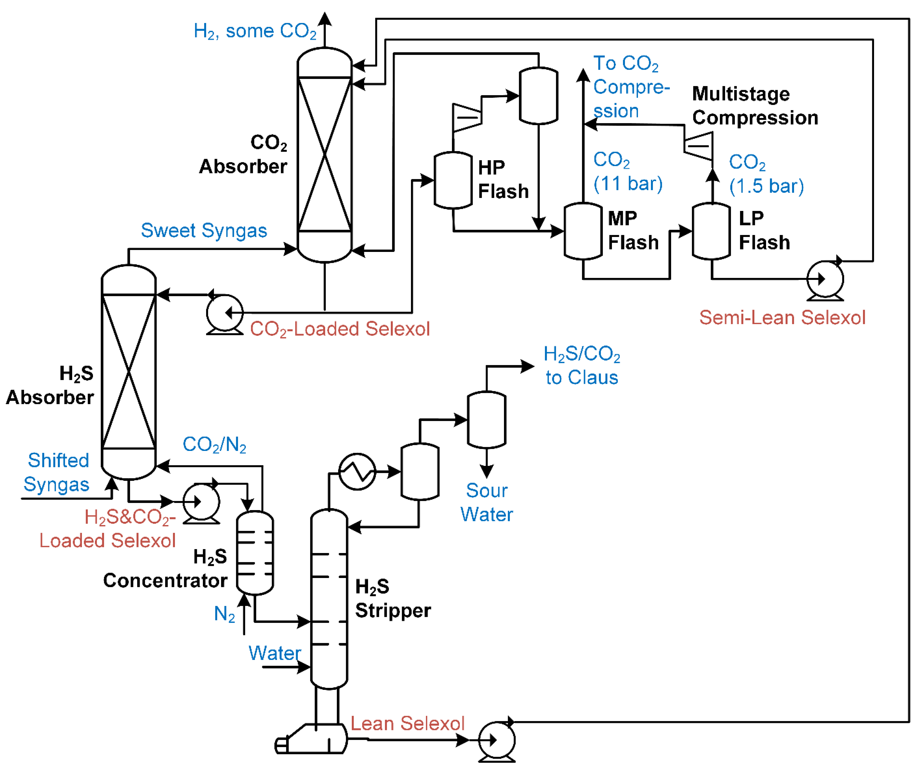
Figure 5.
An example oxyfuel process, based on [41].
Figure 5.
An example oxyfuel process, based on [41].
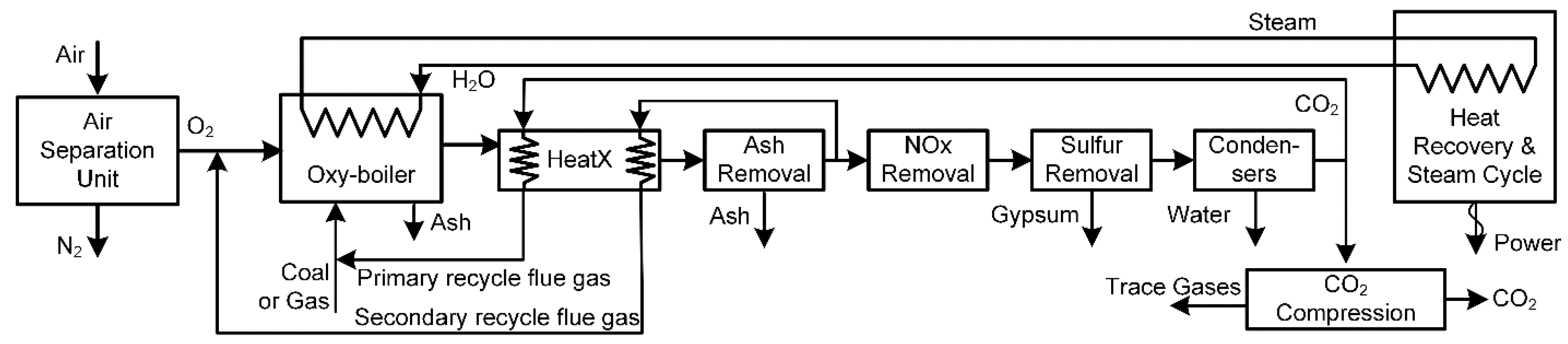
Figure 6.
An example SOFC process from coal (also called integrated gasification fuel cell or IGFC), based on [25].
Figure 6.
An example SOFC process from coal (also called integrated gasification fuel cell or IGFC), based on [25].

Figure 7.
An example chemical looping combustion process using NiO, based on [46].
Figure 7.
An example chemical looping combustion process using NiO, based on [46].

Figure 8.
An example calcium looping process for post-combustion CO2 capture.

Figure 9.
A superstructure of pre-combustion membrane separation processes for coal.
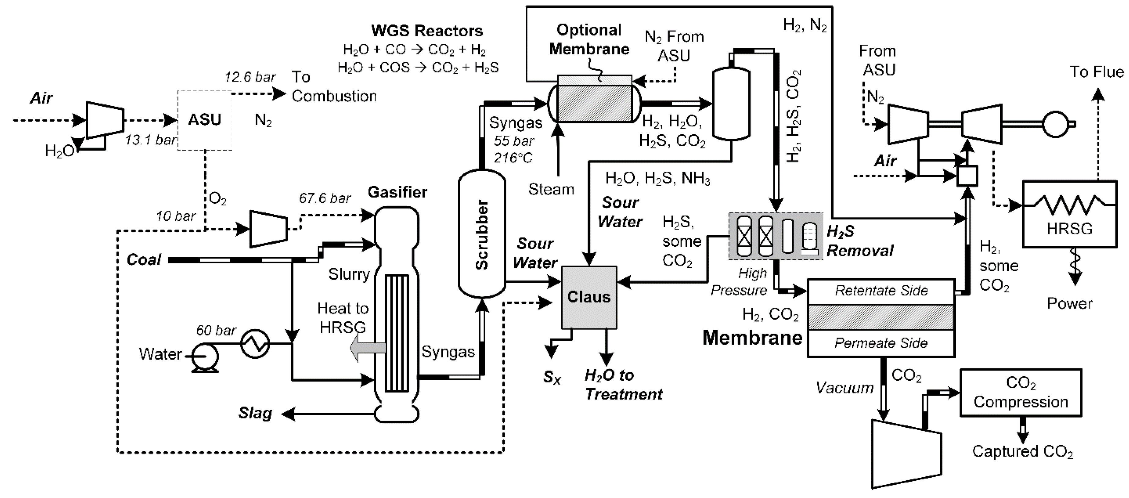
Figure 10.
A superstructure of post-combustion membrane separation processes for coal or gas. Blocks with dashed lines are optional depending on the circumstances. Dark solid squares indicate points at which a design will typically use either Route 1 or Route 2, but not both.
Figure 10.
A superstructure of post-combustion membrane separation processes for coal or gas. Blocks with dashed lines are optional depending on the circumstances. Dark solid squares indicate points at which a design will typically use either Route 1 or Route 2, but not both.
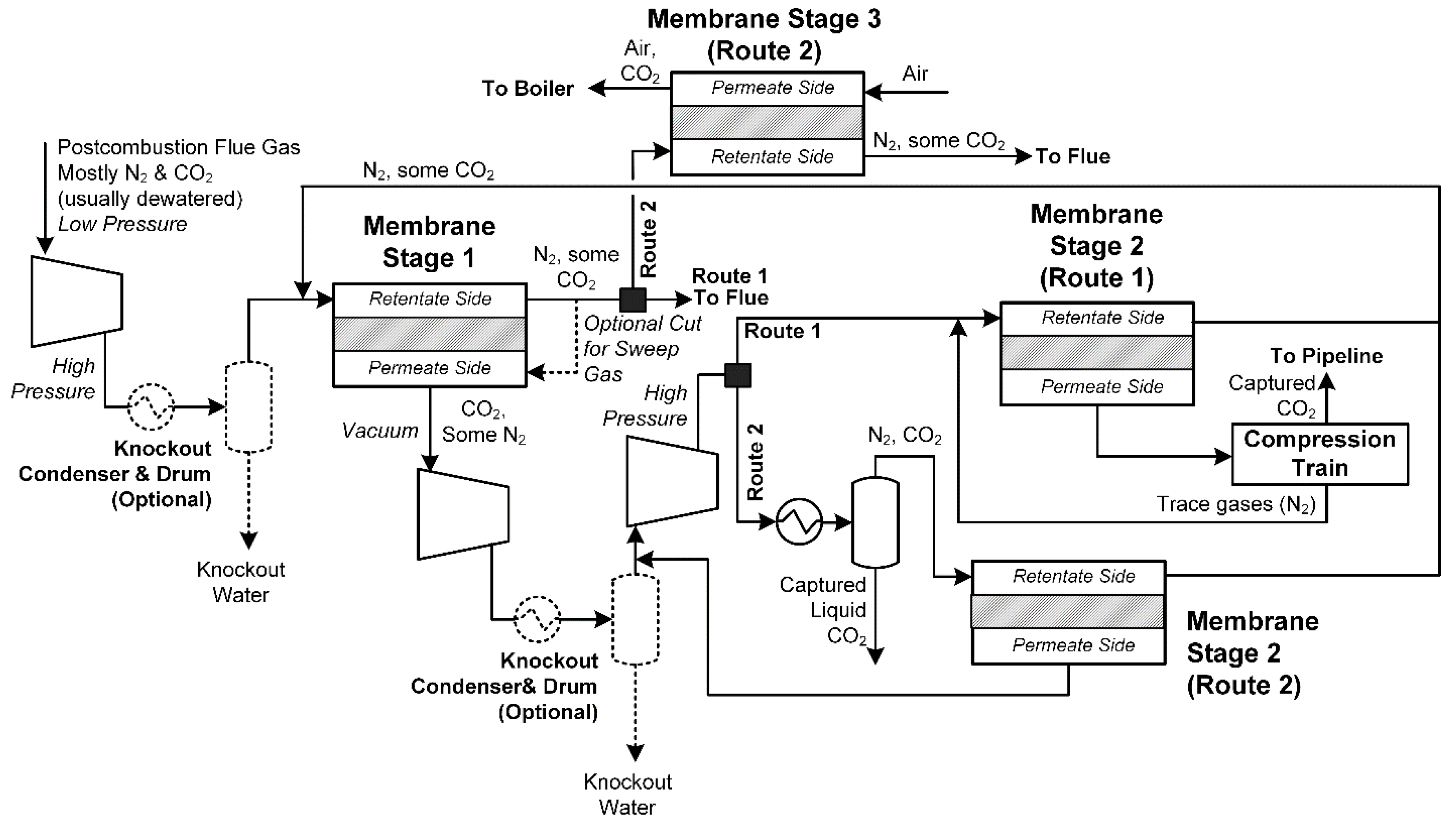
Figure 11.
Scatter plot of fuel unit prices and non-fuel costs for coal-based systems as reported by each study and then converted to $US2016 according to the methods of Section 2. COXY = coal-based oxyfuels, CMEM = coal-based membranes, IGFC = integrated gasification (solid oxide) fuel cell, CaL = calcium looping capture, and CCLC = coal-based chemical looping combustion. The dashed line identifies the “typical” range of the data set as a visual aid only. Note that all plants in the above plot are CCS-enabled.

Figure 12.
Scatter plot of the calculated LCOE at standard conditions of each plant vs. the calculated life cycle greenhouse gas emissions, using as-reported fuel price assumptions. NOXY = natural gas-based oxyfuels, NMEM = natural gas based membranes, NGFC = natural gas (solid oxide) fuel cells, and NCLC = natural gas-based chemical looping combustion.

Figure 13.
Scatter plot of the calculated LCOE at standard conditions of each plant vs. the calculated life cycle greenhouse gas emissions, but using average fuel prices for 2016 instead of as-reported prices. Ellipses are drawn as a visual aid only and do not specifically identify outliers.
Figure 13.
Scatter plot of the calculated LCOE at standard conditions of each plant vs. the calculated life cycle greenhouse gas emissions, but using average fuel prices for 2016 instead of as-reported prices. Ellipses are drawn as a visual aid only and do not specifically identify outliers.

Figure 14.
Scatter plot of the calculated LCOE at standard conditions of each plant vs. the calculated life CCA using as-reported prices, when compared against SCPC and NGCC without CO2 capture. The NGCC baseline plant without CO2 capture is also included as a point of reference. COXY-9 has been removed as an outlier. The straight dashed lines are regression lines for each reference group for the points included. Points with CCA above 120 $US2016/tCO2e were not included in this plot for clarity. Note that all data plotted above are for CCS-enabled plants, except for a single NGCC without CCS plant.

Figure 15.
The average values of the key metrics by process category. COXY-9, COXY-12, and COXY-13 were not included (outliers as described in Section 3.2). Note that all plants in the above plot are CCS-enabled.
Figure 15.
The average values of the key metrics by process category. COXY-9, COXY-12, and COXY-13 were not included (outliers as described in Section 3.2). Note that all plants in the above plot are CCS-enabled.

Figure 16.
The average values of the CCA vs. SCPC without CO2 capture for as-reported fuel prices as a function of the assumed power law parameter .
Figure 16.
The average values of the CCA vs. SCPC without CO2 capture for as-reported fuel prices as a function of the assumed power law parameter .
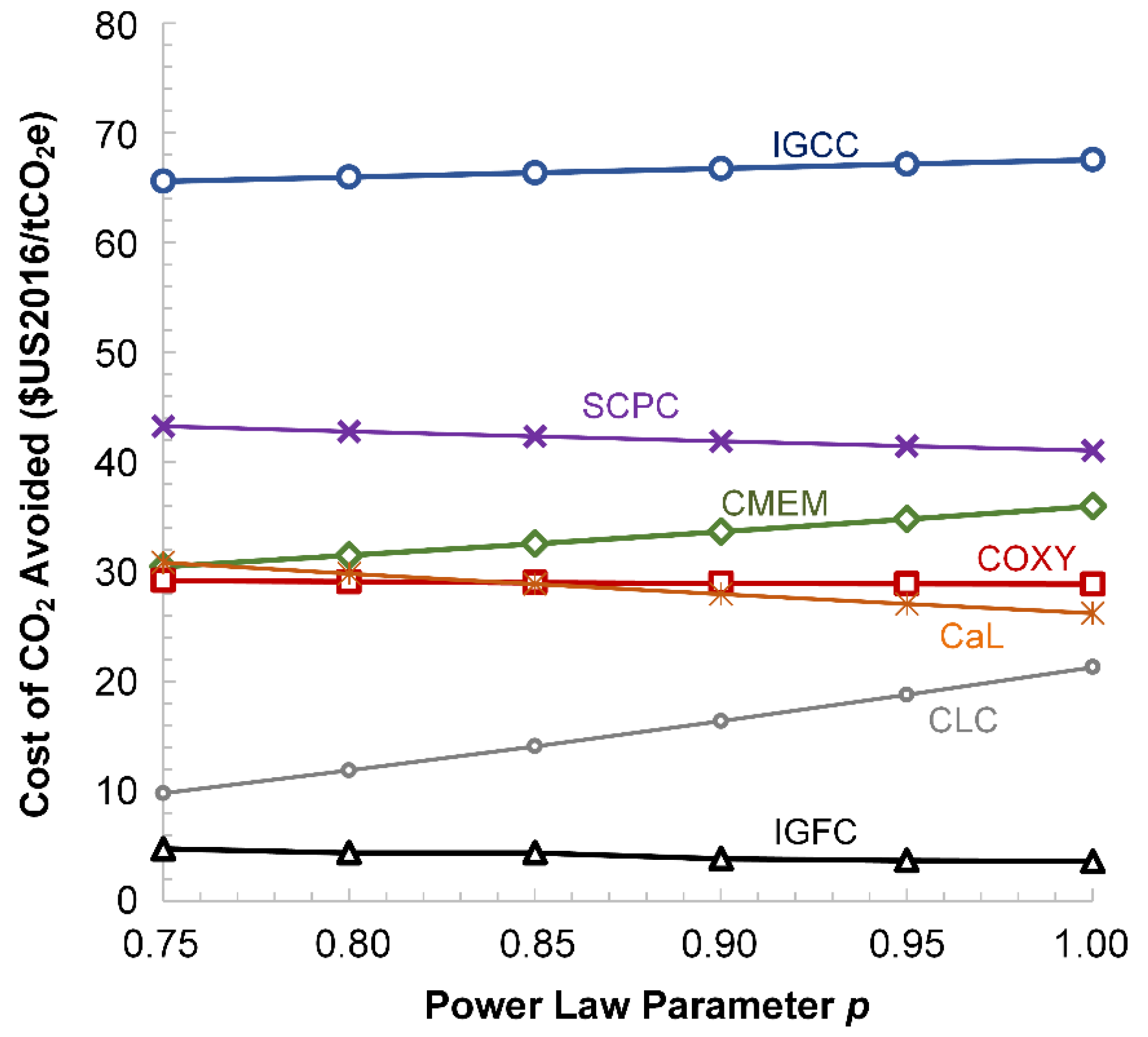

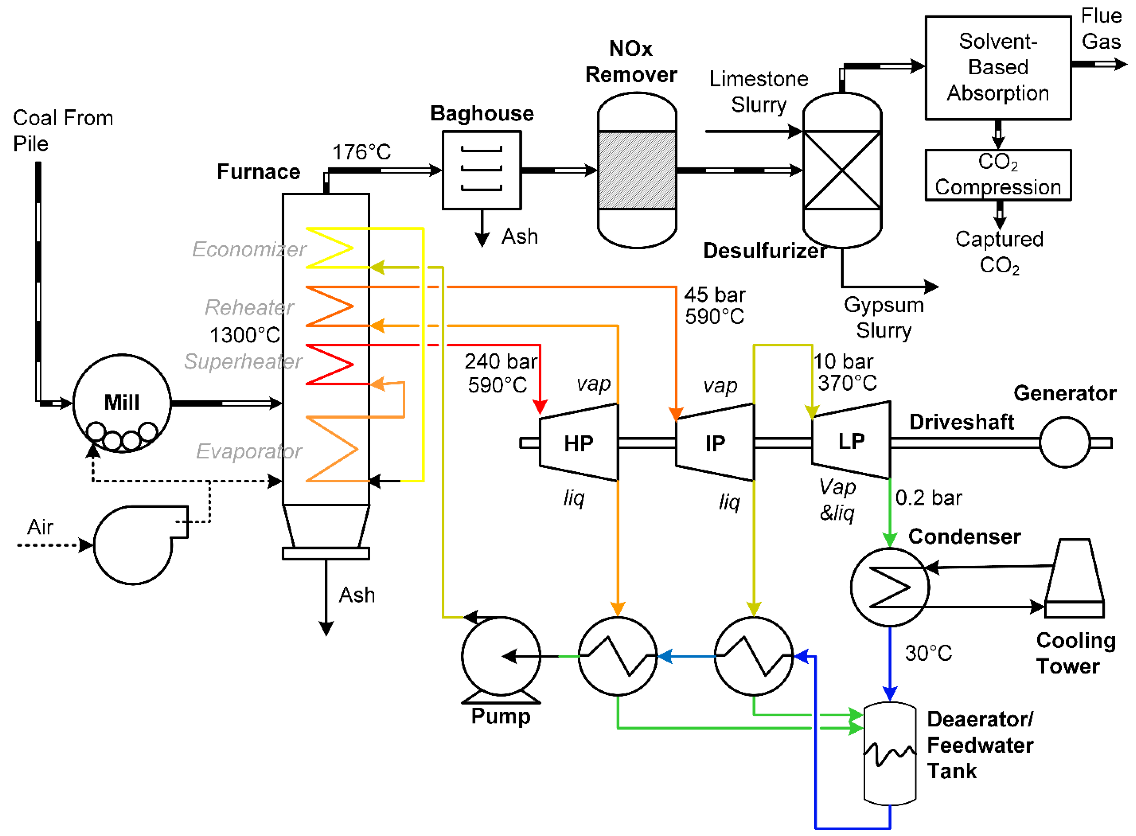
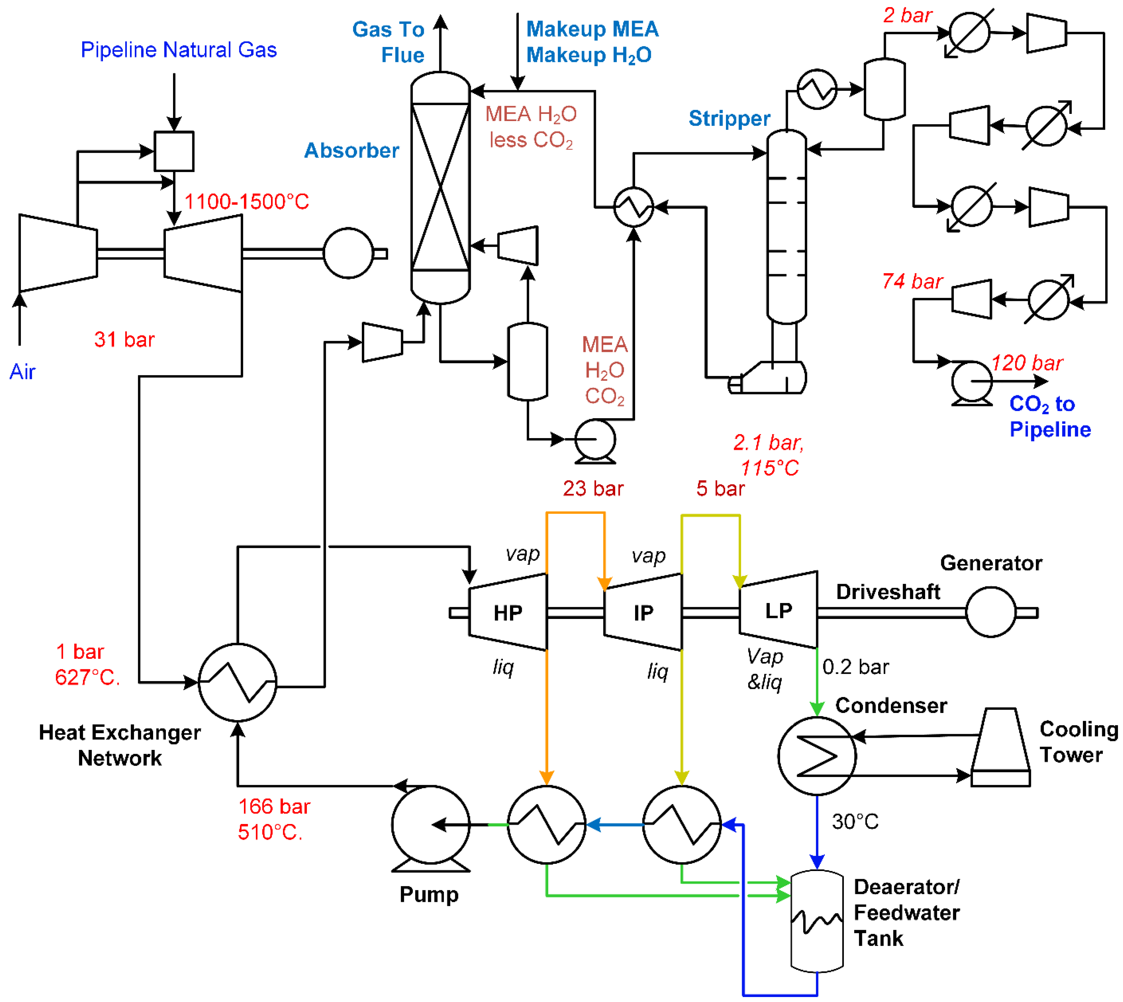
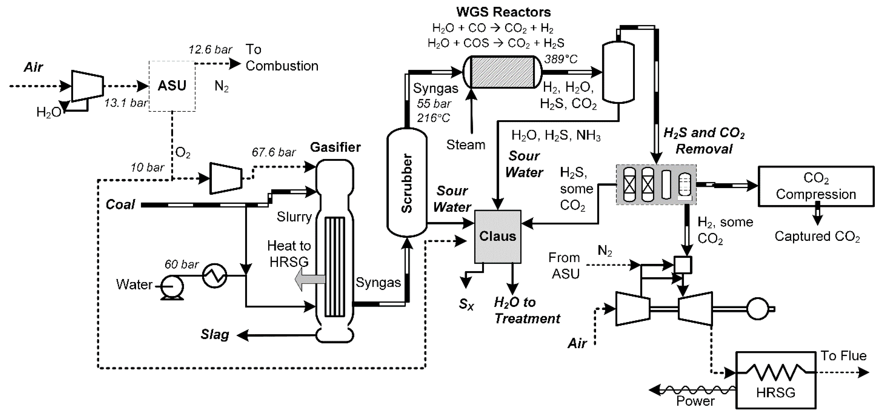
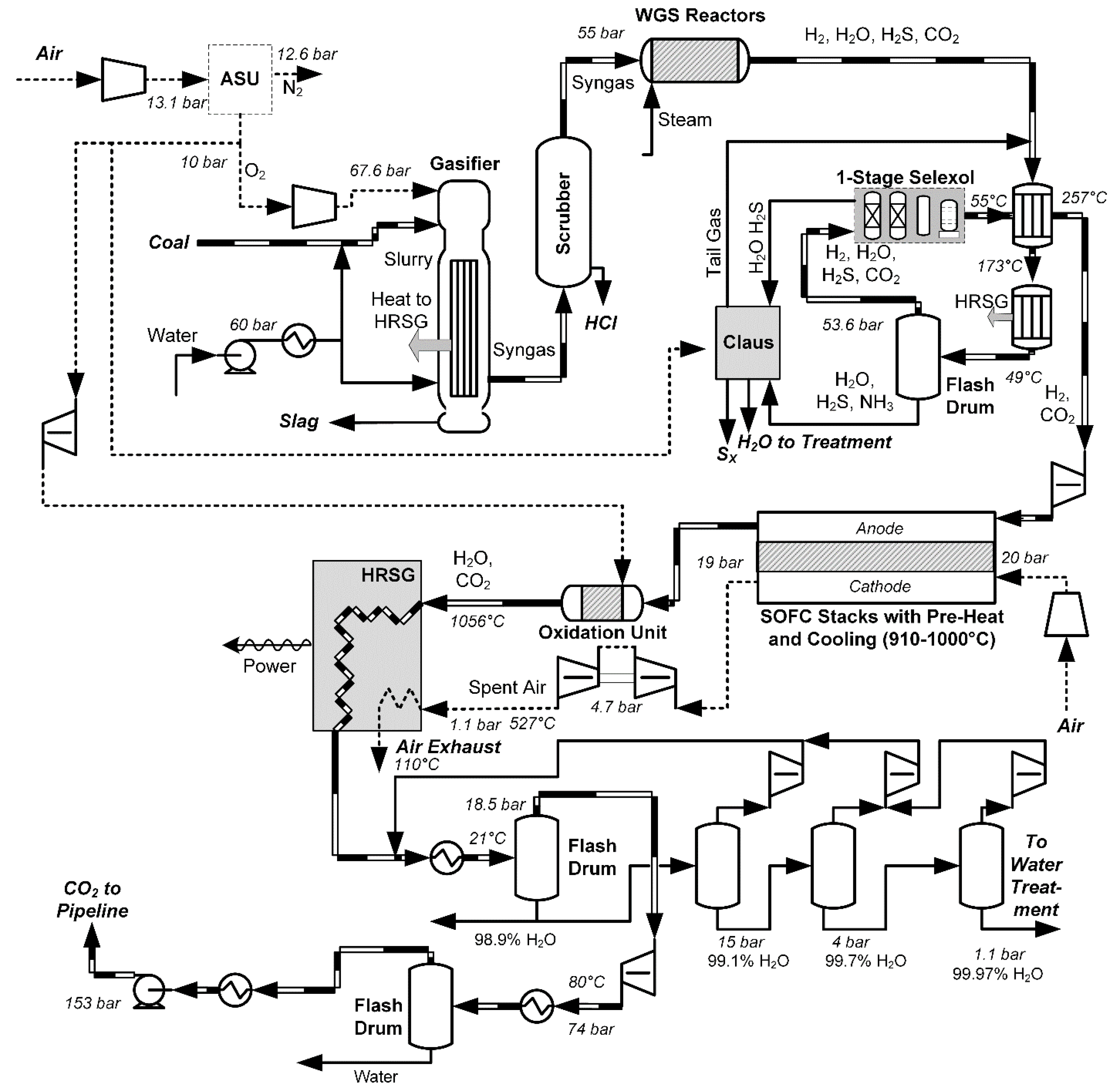
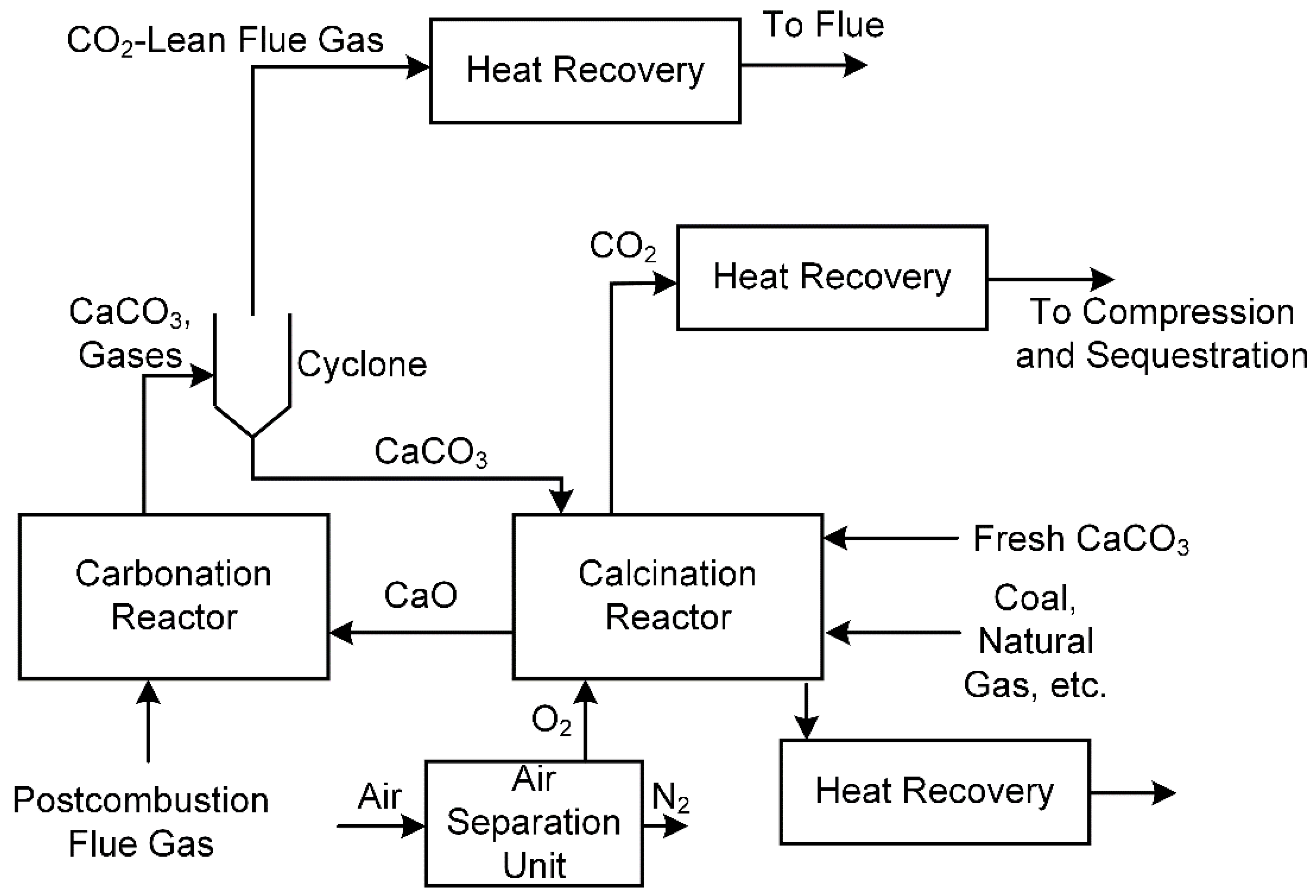
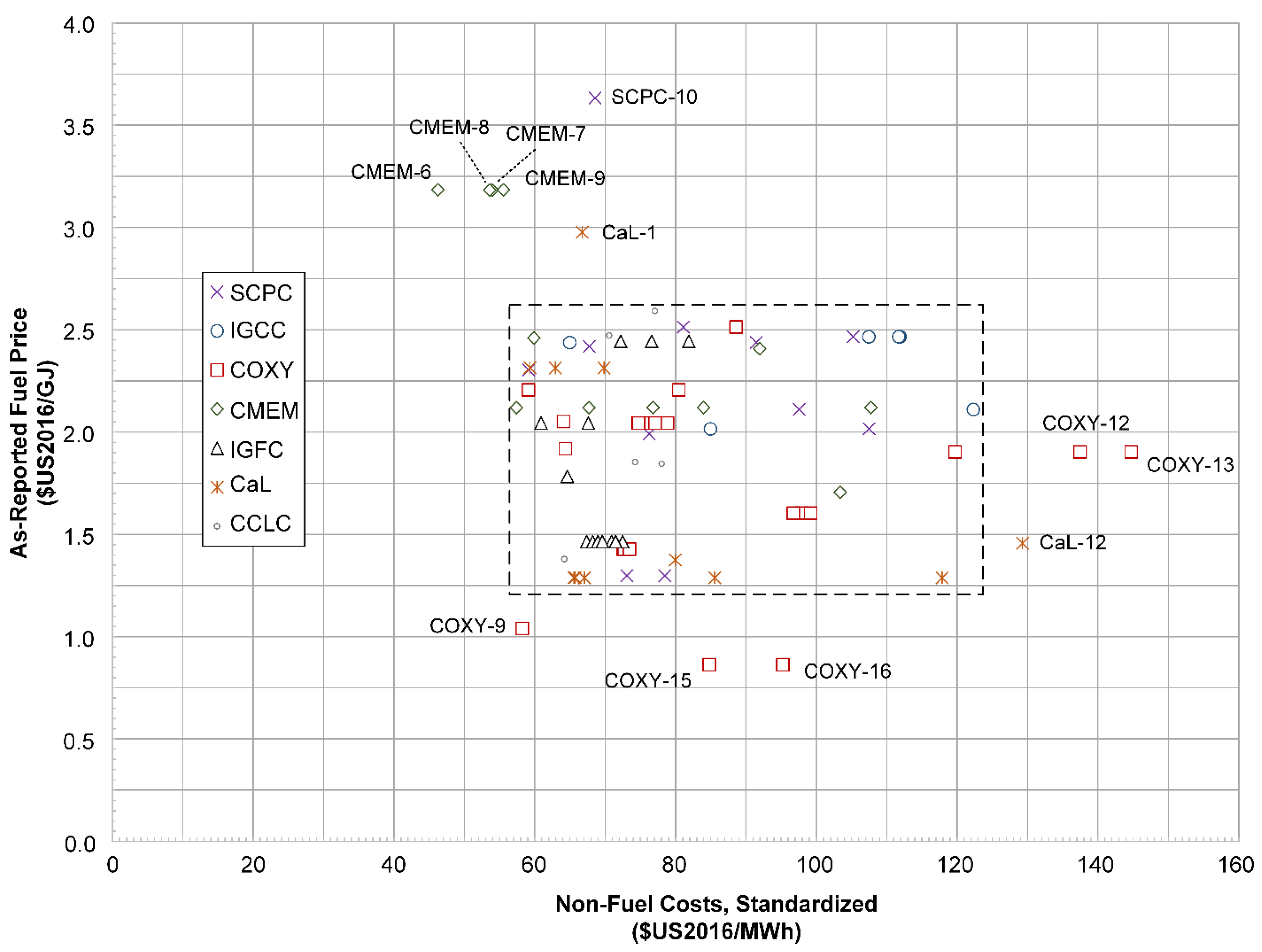
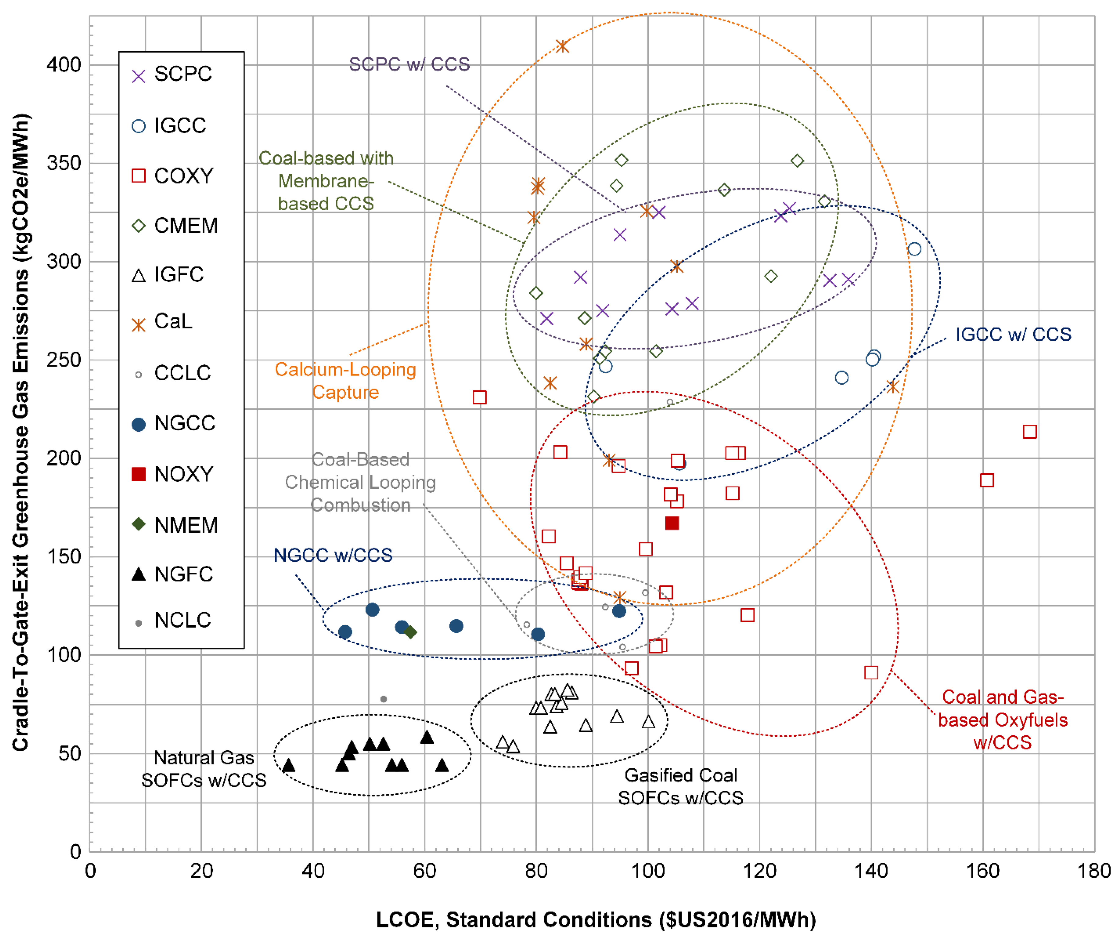
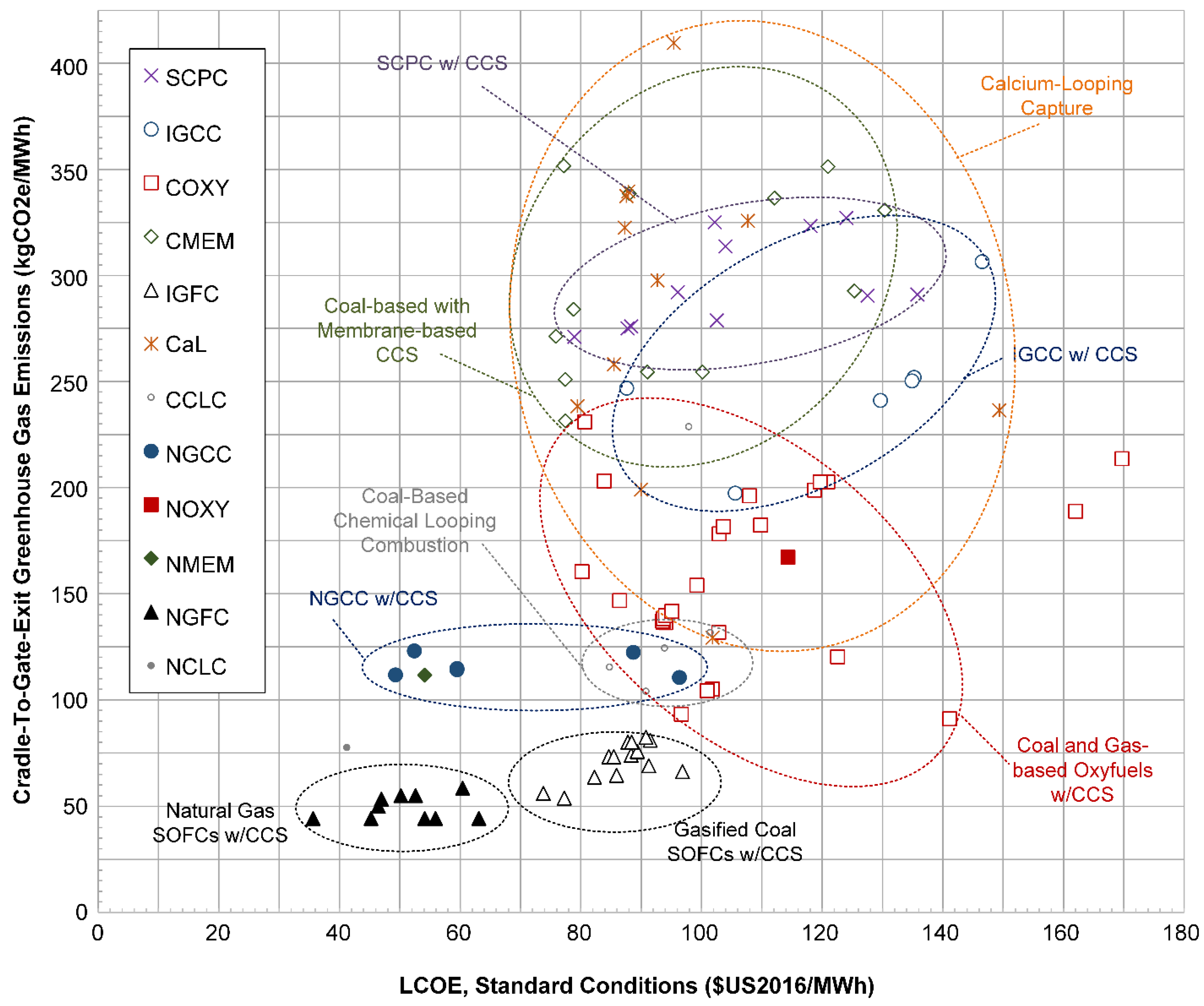
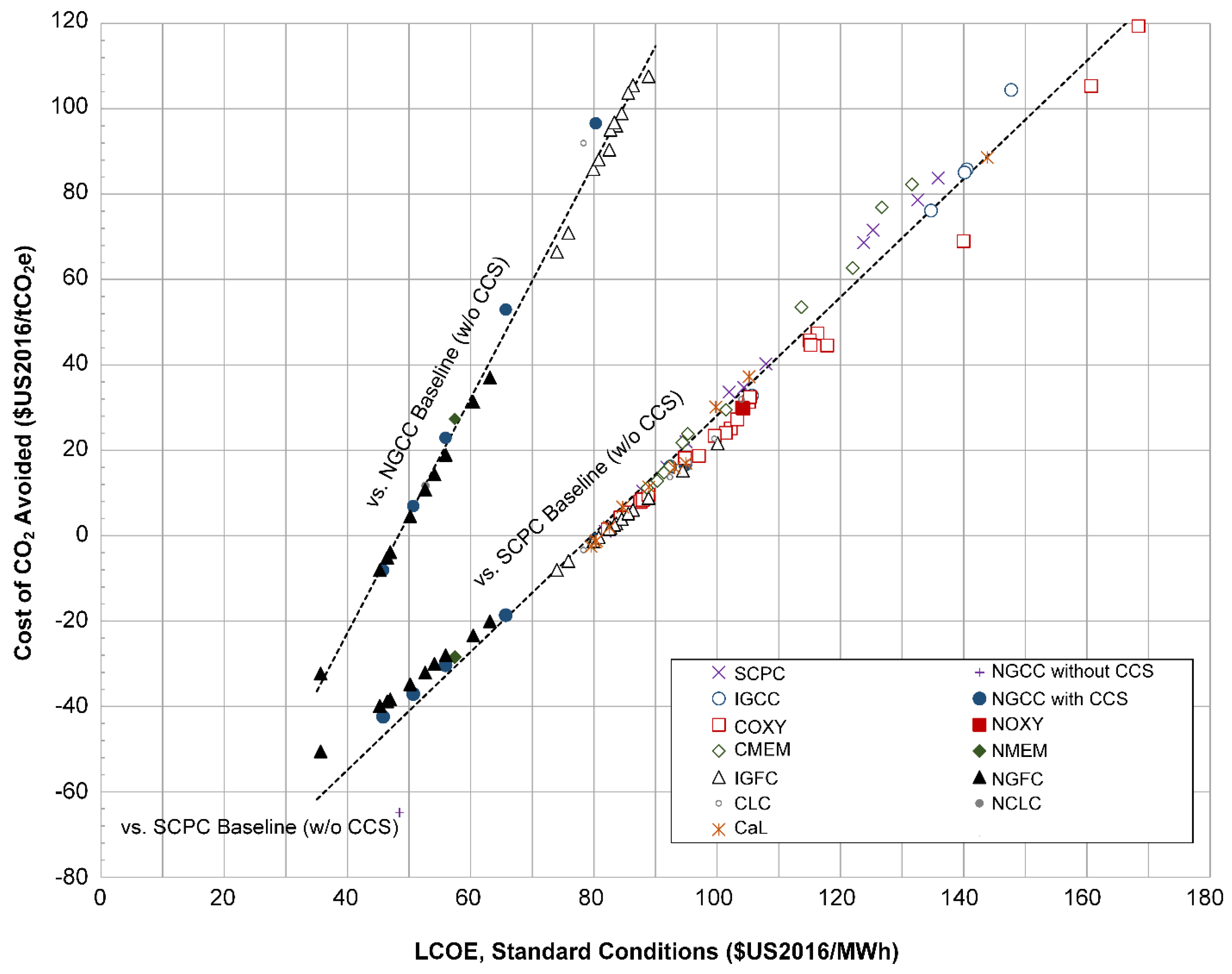
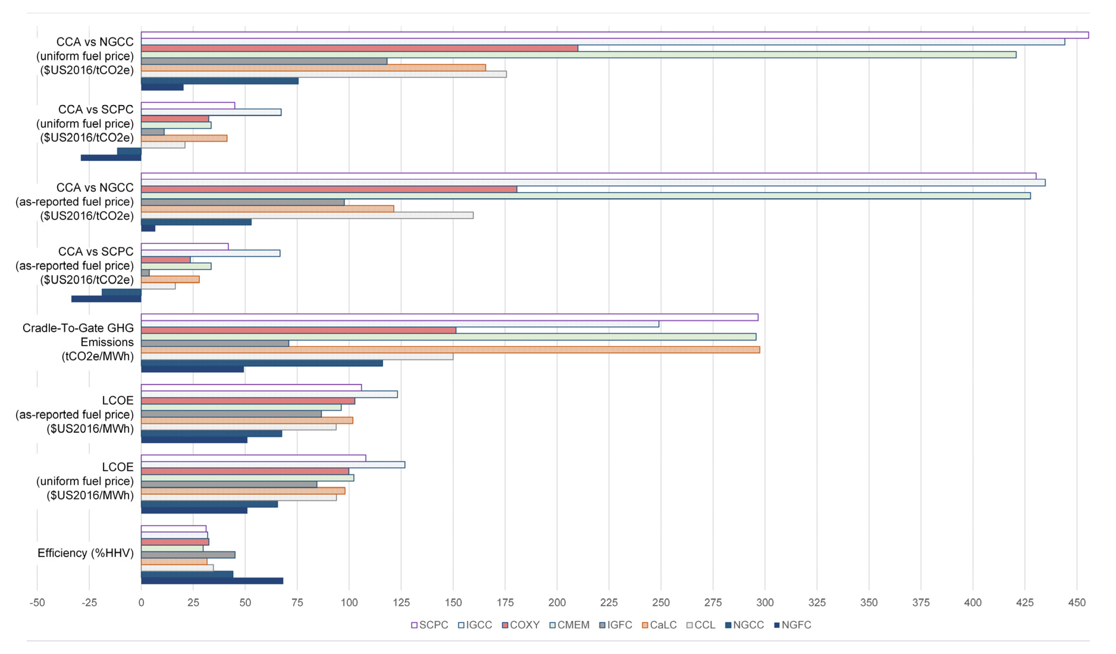
Table 1.
Base cases for coal and gas, representing the current commercial state-of-the-art.
| Property | Supercritical Pulverized Coal Base Case | NGCC Base Case | Units |
|---|---|---|---|
| Fuel Type | Bituminous Coal | Conventional Pipeline Natural Gas | |
| Location | United States | United States | |
| Project Year | 1st Quarter 2016 | 1st Quarter 2016 | |
| Levelized Cost of Electricity (As Reported) | 82.3 | 65.0 | $US2011 per MWh |
| Levelized Cost of Electricity (Adjusted to $2016) | 81.1 | 48.4 | $US2016 per MWh |
| Net Plant Power Output | 550 | 550 | MWe (AC, grid quality, at plant gate, prior to transmission) |
| Electrical Efficiency * | 40.7 | 48.7 | HHV % |
| Direct CO2 Emissions | 868.8 | 373.0 | kgCO2e/MWh of electricity |
| Indirect CO2 Emissions † | 75.6 | 67.3 | kgCO2e/MWh of electricity |
| Cradle-To-Plant-Exit CO2 Emissions | 944.4 | 440.3 | kgCO2e/MWh |
| CO2 Captured | 0% | 0% | |
| Fuel Price | 2.47 | 3.37 | $US2016 per GJ |
| Fuel Price (as reported) | 2.78 | 5.69 | $US2011 per GJ |
| Non-Fuel Costs | 59.3 | 23.6 | $US2016 per MWh |
| Non-Fuel Costs (as reported) | 57.7 | 22.9 | $US2011 per MWh |
| CCA by switching from SCPC base case to NGCC base case (with no carbon capture) | −64.8 | $US2016/tCO2e | |
| Reference | [6] | [52] | |
* Electrical efficiency is defined as the net electricity produced (AC, grid quality) at the plant gate prior to transmission divided by the higher heating value of the fuel consumed, including any parasitic loads within the plant boundary. † These are the cradle-to-gate-entrance CO2 emissions of producing, processing, and delivering the fuel to the plant. See Section 2.4 for details.
Table 2.
Coal-fired power plants surveyed in the meta-study, with key metrics shown. For other metrics and intermediate calculations, please see the Microsoft Excel file included with the supplementary material. Notes: tCO2e is in metric tonnes. LCU = local currency unit. Converted to Standard means that the plant has been converted to the standard size, project year, and locale according to the methods described in Section 2.
| LCOE (Using As-Reported Fuel Prices) | CCA (Converted to Standard Form Using As-Reported Fuel Prices, $US2016/tCO2e) | ||||||||||
|---|---|---|---|---|---|---|---|---|---|---|---|
| Tag | Ref. | Project Year, LCU | Technology | Reported Capacity (MW) | Reported Efficiency (%HHV) | Reported (LCU/MWh) | Converted to Standard ($/MWh) | CO2 Captured (%) | Lifecycle CO2 Emissions (tCO2e/MWh) | Compared to SCPC Baseline | Compared to NGCC Baseline |
| SCPC-1 | [9] | $2011 | Solvent Based—EconFG+ | 550 | 32.5 | 133.2 | 132.6 | 90 | 0.290 | 78.7 | 561.1 |
| SCPC-2 | [66] | $2013 | Solvent Based | 525 | 27.4 | 129.5 | 125.3 | 90 | 0.327 | 71.6 | 678.7 |
| SCPC-3 | [67] | €2010 | Solvent Based—Advanced amine | 837 | 36.1 | 73 | 91.8 | 90 | 0.275 | 16.0 | 262.6 |
| SCPC-4 | [68] | €2013 | Solvent Based—Cansolv | 822 | 33.8 | 86.3 | 107.9 | 90 | 0.279 | 40.2 | 368.0 |
| SCPC-5 | [69] | $2010 | Solvent Based—Amine | 546 | 27.2 | 122 | 123.8 | 90 | 0.323 | 68.7 | 643.5 |
| SCPC-6 | [70] | €2010 | Solvent Based—Advanced Amine | 616 | 36.5 | 70.3 | 81.8 | 90 | 0.271 | 1.1 | 197.4 |
| SCPC-7 | [71] | $2006 | Solvent based-Chilled Ammonia | 548.7 | 28.4 | 80.8 | 95.0 | 90 | 0.314 | 22.0 | 367.4 |
| SCPC-8 | [71] | $2006 | Solvent based-Chilled Ammonia | 549.3 | 31.5 | 74.7 | 87.9 | 90 | 0.292 | 10.4 | 266.5 |
| SCPC-9 | [14] | $2007 | Solvent based-Chilled Ammonia | 558.7 | 27.9 | 100.2 | 102.0 | 90 | 0.325 | 33.7 | 464.2 |
| SCPC-10 | [12] | €2008 | Solvent based-Chilled Ammonia | 614 | 36.6 | 82.3 | 104.3 | 88.4 | 0.276 | 34.7 | 339.9 |
| SCPC-11 | [72] | £2011 | Solvent Based-Amine | 519 | 25.6 | 102 | 135.9 | 94 | 0.247 | 16.2 | 227.1 |
| IGCC-1 | [73] | $2011 | Solvent Based-Selexol | 543 | 32.6 | 135.4 | 134.7 | 90 | 0.291 | 83.8 | 585.2 |
| IGCC-2 | [73] | $2011 | Solvent Based-Selexol | 514 | 31 | 141.9 | 140.5 | 90 | 0.241 | 76.2 | 432.7 |
| IGCC-3 | [73] | $2011 | Solvent Based-Selexol | 497 | 31.2 | 141.9 | 140.2 | 90 | 0.252 | 85.8 | 488.7 |
| IGCC-4 | [66] | $2013 | Data not available | 500 | 29.9 | 152.6 | 147.7 | 86 | 0.250 | 85.1 | 482.6 |
| IGCC-5 | [69] | $2010 | Solvent Based-Selexol NS | 694 | 32 | 90 | 92.4 | 90 | 0.307 | 104.4 | 742.1 |
| IGCC-6 | [72] | £2011 | Solvent Based—Shift + Selexol | 455 | 35.1 | 79.7 | 105.6 | 94 | 0.197 | 32.8 | 235.4 |
| CMEM-1 | [74] | $2010 | Membrane—2 stage | 550 | 25.7 | 112 | 113.7 | 90 | 0.336 | 53.5 | 628.1 |
| CMEM-2 | [75] | €2008 | Membrane—3 stage | 754 | 33 | 94 | 122.0 | 90 | 0.293 | 62.7 | 498.3 |
| CMEM-3 | [76] | $2010 | Membrane—Two stage two step with air sweep | 550 | 25.7 | 94.1 | 94.3 | 90 | 0.339 | 21.8 | 451.2 |
| CMEM-4 | [77,78] | $2007 | H2-CO2 selective membrane with sweep gas | 556 | 31 | 90.48 | 92.3 | 90 | 0.254 | 16.2 | 236.1 |
| CMEM-5 | [79] | $2007 | 2 stages membrane with argon as sweep gas (Amine-containing—membranes synthesized and tested) | 550 | 31 | 100 | 101.4 | 90 | 0.254 | 29.5 | 285.2 |
| CMEM-6 | [80] | €2015 | Cascade Membrane system-polymeric | 439 | 23.38 | 85.9 | 95.3 | 90 | 0.352 | 23.8 | 528.0 |
| CMEM-7 | [80] | €2015 | 3 end membrane integration-ceramic | 492 | 33.06 | 77.3 | 88.6 | 90 | 0.271 | 11.2 | 237.7 |
| CMEM-8 | [80] | €2015 | Microporous ceramic membrane—H2 selective | 316 | 30.37 | 82 | 91.4 | 90 | 0.251 | 14.8 | 226.6 |
| CMEM-9 | [80] | €2015 | Microporous ceramic membrane—soar WGS membrane | 316 | 33.01 | 80.6 | 90.3 | 90 | 0.231 | 12.9 | 200.3 |
| CMEM-10 | [81] | €2015 | Integrated WGS membrane reactor | 286 | 32 | 86 | 104.6 | 81 | 0.331 | 38.3 | 513.1 |
| CMEM-11 | [82] | €2015 | Two stages membrane | 350 | 24.9 | 107.2 | 123.3 | 90 | 0.351 | 71.1 | 841.2 |
| CMEM-12 | [83] | €2014 | Membrane-cryogenic | 427 | 33.82 | 65.5 | 80.0 | 90 | 0.284 | −1.8 | 201.7 |
| CCRY-1 | [15] | €2012 | Cryogenic | 699 | 33.06 | 99.7 | 124.3 | 90 | 0.286 | 65.6 | 491.2 |
| COXY-1 | [84] | €2015 | Oxy-fuel | 475 | 34.31 | 70.06 | 82.3 | 91 | 0.160 | 1.5 | 120.9 |
| COXY-2 | [84] | €2015 | Oxy-fuel | 475 | 32.2 | 88.54 | 105.1 | 90 | 0.178 | 31.4 | 216.3 |
| COXY-3 | [85] | €2012 | Oxy-fuel | 826 | 34.72 | 71.7 | 88.1 | 94 | 0.136 | 8.6 | 130.3 |
| COXY-4 | [85] | €2012 | Oxy fuel with 10% air added | 826 | 34.67 | 71.4 | 87.6 | 94 | 0.137 | 8.1 | 129.0 |
| COXY-5 | [85] | €2012 | Oxy fuel with 20% air added | 826 | 34.51 | 71.3 | 87.5 | 94 | 0.137 | 7.9 | 128.8 |
| COXY-6 | [85] | €2012 | Oxy fuel with 30% air added | 826 | 34.25 | 71.4 | 87.6 | 94 | 0.138 | 8.0 | 129.5 |
| COXY-7 | [85] | €2012 | Oxy fuel with 40% air added | 826 | 33.88 | 71.7 | 87.9 | 94 | 0.140 | 8.4 | 131.2 |
| COXY-8 | [85] | €2012 | Oxy fuel with 50% air added | 826 | 33.41 | 72.5 | 88.8 | 94 | 0.142 | 9.6 | 135.3 |
| COXY-9 | [86] | €2007 | Oxy-fuel | 357 | 32.29 | 57.5 | 69.8 | 90 | 0.231 | −15.8 | 102.2 |
| COXY-10 | [87] | $2009 | Oxy-fuel | 601 | 32.74 | 82.3 | 85.4 | 93 | 0.147 | 5.4 | 126.1 |
| COXY-11 | [88] | €2014 | Oxy-fuel with compression and dehydration | 400 | 33.81 | 116.3 | 140.0 | 100 | 0.091 | 69.0 | 262.1 |
| COXY-12 | [88] | €2014 | Oxy-fuel with double flash purification | 400 | 29.51 | 133.5 | 160.7 | 92 | 0.189 | 105.3 | 446.2 |
| COXY-13 | [88] | €2014 | Oxy-fuel with distillation purification | 400 | 28.99 | 139.8 | 168.4 | 90 | 0.214 | 119.4 | 529.0 |
| COXY-14 | [89] | €2009 | Oxy-fuel | 630 | 36.6 | 67.2 | 84.3 | 90 | 0.203 | 4.3 | 151.1 |
| COXY-15 | [68] | $2007 | Oxy-fuel (Case: S12F) | 550 | 31.2 | 96 | 94.7 | 90.8 | 0.196 | 18.2 | 189.6 |
| COXY-16 | [68] | $2007 | Oxy-fuel (Case: S22F) | 550 | 30.8 | 106.9 | 105.3 | 90.9 | 0.199 | 32.5 | 235.5 |
| COXY-17 | [66] | $2013 | Oxy-fuel (Boiler type & Coal rank: USC-subbit) | 509 | 31.5 | 119.8 | 116.3 | 90 | 0.203 | 47.4 | 285.5 |
| COXY-18 | [66] | $2013 | Oxy-fuel (Boiler type & Coal rank: SCPC-bit) | 510 | 31 | 121.4 | 117.8 | 98 | 0.120 | 44.6 | 216.9 |
| COXY-19 | [66] | $2013 | Oxy-fuel (Boiler type & Coal rank: SCPC-bit) | 501 | 31.5 | 118.7 | 115.0 | 90 | 0.203 | 45.7 | 280.3 |
| COXY-20 | [68] | €2013 | Oxy-fuel (Boiler type & Coal rank: USC-subbit) | 833 | 34.1 | 91.6 | 115.1 | 90 | 0.182 | 44.6 | 258.4 |
| COXY-21 | [90] | $2007 | Oxy-combustion Supercritical PC with CO2 Capture | 550 | 29.3 | 100.7 | 102.2 | 99.5 | 0.105 | 25.1 | 160.4 |
| COXY-22 | [90] | $2007 | Oxy-combustion Supercritical PC with CO2 Capture | 555 | 29.5 | 99.8 | 101.4 | 99.4 | 0.104 | 24.1 | 157.5 |
| COXY-23 | [90] | $2007 | Oxy-combustion Supercritical PC with CO2 Capture | 549 | 29.3 | 101.8 | 103.3 | 96.9 | 0.132 | 27.2 | 177.7 |
| COXY-24 | [90] | $2007 | Oxy-combustion Supercritical PC with CO2 Capture | 549 | 29.2 | 102.6 | 104.0 | 85.5 | 0.182 | 30.1 | 214.9 |
| COXY-25 | [90] | $2007 | Oxy-combustion Ultra-supercritical PC with CO2 Capture | 550 | 33 | 95.9 | 97.0 | 99.4 | 0.093 | 18.7 | 140.0 |
| COXY-26 | [90] | $2007 | Oxy-combustion Ultra-supercritical PC with CO2 Capture | 545 | 32.7 | 98.6 | 99.6 | 93.2 | 0.154 | 23.4 | 178.7 |
| IGFC-1 | [44] | $2011 | Uses WGS to minimize CO content in SOFC feed | 719 | 42 | 78 | 79.9 | 100 | 0.073 | −1.3 | 85.8 |
| IGFC-2 | [44] | $2011 | IGFC-1 but with seasonal SOFC shutdowns to preserve life during low-demand deasons | 719 | 42 | 78.8 | 80.8 | 100 | 0.073 | −0.4 | 88.1 |
| IGFC-3 | [44] | $2011 | IGFC-1 with integrated energy storage | 719 | 41.5 | 81.5 | 83.6 | 100 | 0.074 | 2.9 | 96.1 |
| IGFC-4 | [44] | $2011 | IGFC-2 with integrated energy storage | 719 | 40.6 | 82.4 | 84.5 | 100 | 0.076 | 3.9 | 99.0 |
| IGFC-5 | [44] | $2011 | Uses coal syngas directly in SOFC with no WGS | 719 | 38.4 | 80.8 | 82.7 | 100 | 0.080 | 1.8 | 95.1 |
| IGFC-6 | [44] | $2011 | IGFC-5 with seasonal SOFC shutdowns | 719 | 38.41 | 81.4 | 83.3 | 100 | 0.080 | 2.5 | 96.8 |
| IGFC-7 | [44] | $2011 | IGFC-5 with integrated energy storage | 719 | 38 | 84.3 | 86.3 | 100 | 0.081 | 6.1 | 105.5 |
| IGFC-8 | [44] | $2011 | IGFC-5 with integrated energy storage | 719 | 37.4 | 83.6 | 85.6 | 100 | 0.082 | 5.2 | 103.7 |
| IGFC-9 | [91] | $2007 | Atm-Pressure IGFC Plant | 253 | 49.4 | 88 | 82.5 | 99 | 0.064 | 1.6 | 90.4 |
| IGFC-10 | [91] | $2007 | Pressurized IGFC | 253 | 56.2 | 79 | 74.0 | 99 | 0.056 | −8.0 | 66.5 |
| IGFC-11 | [92] | $2007 | Partially methanated Syngas IGFC (TREMP) | 847 | 48.32 | 96.3 | 100.1 | 99 | 0.066 | 21.6 | 138.1 |
| IGFC-12 | [92] | $2007 | Partially methanated Syngas IGFC (HICOM) | 925 | 52.81 | 84.8 | 88.9 | 99 | 0.065 | 8.8 | 107.6 |
| IGFC-13 | [92] | $2007 | IGFC-DIRECT | 865 | 49.36 | 90.6 | 94.4 | 99 | 0.069 | 15.2 | 123.9 |
| IGFC-14 | [93] | $2006 | Liquid-tin anode SOFC | 93.9 | 57.2 | 71 | 75.9 | 100 | 0.054 | −5.9 | 70.9 |
| CaL-1 | [48] | €2005 | CaO Looping | 621 | 27.87 | 48.3 | 105.2 | 85 | 0.298 | 37.2 | 397.8 |
| CaL-2 | [49] | €2009 | CaO Looping w/o heat recovery | 446 | 18.59 | 102 | 142.8 | 85 | 0.476 | 131.8 | −2650.7 |
| CaL-3 | [49] | €2009 | CaO Looping with Combined Cycle Design 1 | 594.8 | 24.24 | 59.5 | 84.7 | 85 | 0.410 | 6.7 | 1179.7 |
| CaL-4 | [49] | €2009 | CaO Looping with Combined Cycle Design 2 | 446 | 32.67 | 71 | 99.8 | 85 | 0.326 | 30.2 | 447.9 |
| CaL-5 | [49] | €2009 | CaO Looping with Combined Cycle Design 3 | 594.8 | 33.54 | 55.5 | 79.6 | 85 | 0.323 | −2.5 | 264.3 |
| CaL-6 | [49] | €2009 | CaO Looping with Combined Cycle Design 4 | 846 | 35.26 | 54.3 | 80.2 | 85 | 0.337 | −1.5 | 308.8 |
| CaL-7 | [49] | €2009 | CaO Looping with Combined Cycle Design 5 | 835.3 | 34.78 | 54.5 | 80.4 | 85 | 0.340 | −1.2 | 317.5 |
| CaL-8 | [50] | $2011 | CaO Looping | 932.9 | 33.10 | 90.68 | 94.9 | 99 | 0.129 | 16.9 | 149.5 |
| CaL-9 | [47] | €2013 | Sub-critical pulverized coal with CaO Looping | 558.9 | 32.06 | 73.77 | 88.9 | 92.25 | 0.258 | 11.4 | 222.2 |
| CaL-10 | [47] | €2013 | SCPC with CaO Looping | 544.22 | 35.91 | 68.41 | 82.5 | 92.66 | 0.238 | 2.0 | 168.6 |
| CaL-11 | [47] | €2013 | IGCC with CaO Looping | 558.08 | 35.97 | 76.48 | 93.0 | 92.95 | 0.199 | 16.0 | 184.7 |
| CaL-12 | [94] | $2012 | SCPC with CaO Looping | 1060 | 36.00 | 136.85 | 143.8 | 90 | 0.236 | 88.6 | 467.8 |
| CLC-1 | [95] | $2003 | Chemical Looping Combustion | 164.484 | 30.88 | 58.4 | 99.5 | 90–99 | 0.132 | 22.7 | 165.6 |
| CLC-2 | [95] | $2003 | Chemical Looping Gasification | 256.83 | 36.90 | 52.2 | 92.4 | 90–99 | 0.124 | 13.7 | 139.0 |
| CLC-3 | [96] | $2007 | Syngas Chemical Looping | 346.8 | 34.70 | 100.7 | 103.9 | 90 | 0.229 | 31.9 | 262.2 |
| CLC-4 | [97] | $2011 | Coal Direct Chemical Looping (CDCL) Retrofit to Pulverized Coal Power Plants for In-Situ CO2 Capture | 548 | 35.20 | 78.4 | 78.3 | 97 | 0.115 | −3.4 | 91.9 |
| CLC-5 | [98] | $2011 | Alstom Limestone Chemical Looping plant using Fast CFB transport reactors | 550 | 35.80 | 96.7 | 95.4 | 97 | 0.104 | 17 | 139.7 |
Table 3.
Gas-fired power plants surveyed in the meta-study, with key metrics shown. For other metrics and intermediate calculations, please see the Microsoft Excel file included with the supplementary material. Notes: tCO2e is in metric tonnes. LCU = local currency unit (given in third column). Converted to Standard means that the plant has been converted to the standard size, project year, and locale according to the methods described in Section 2.
| LCOE (Using As-Reported Fuel Prices) | CCA (Converted to Standard form Using As-Reported Fuel Prices, $US2016/tCO2e) | ||||||||||
|---|---|---|---|---|---|---|---|---|---|---|---|
| Tag | Ref. | Project Year, LCU | Technology | Reported Capacity (MW) | Reported Efficiency (%HHV) | Reported (LCU/MWh) | Converted to Standard ($/MWh) | CO2 Captured (%) | Lifecycle CO2 Emissions (tCO2e/MWh) | Compared to SCPC Baseline | Compared to NGCC Baseline |
| NGCC-1 | [9] | $2011 | Solvent Based—Econamine FG+ | 559 | 45.7 | 83.3 | 65.7 | 90 | 0.115 | −18.6 | 53.0 |
| NGCC-2 | [99] | €2011 | Solvent Based—MEA | 789 | 46.1 | 74.8 | 54.8 | 90 | 0.114 | −31.6 | 19.6 |
| NGCC-3 | [99] | €2011 | Solvent Based—Advanced Amine | 804 | 47 | 68.9 | 47.8 | 90 | 0.112 | −40.0 | −1.9 |
| NGCC-4 | [100] | $2007 | Solvent Based—Econamine FG+ | 448.9 | 42.6 | 84.2 | 50.6 | 90 | 0.123 | −37.1 | 7.0 |
| NGCC-5 | [100] | $2013 | Solvent Based—Amine | 485 | 42.4 | 112 | 94.8 | 90 | 0.122 | 16.7 | 145.9 |
| NGCC-6 | [72] | £2011 | Solvent Based—Amine | 389 | 40.8 | 108.41292 | 80.3 | 94 | 0.110 | −1.0 | 96.6 |
| NMEM-1 | [101] | $2012 | Solvent supported CO2 membrane | 376.9 | 48 | 63.8 | 57.4 | 90 | 0.112 | −28.5 | 27.3 |
| NOXY-1 | [102] | $2011 | Oxy-fuel | 227.6 | 31.22 | 123.7 | 104.3 | 90 | 0.167 | 29.8 | 204.4 |
| NGFC-1 | [103] | $2007 | SOFC base case ($1000/kW installed) | 693 | 74 | 64.5 | 45.2 | 100 | 0.044 | −39.9 | −8.1 |
| NGFC-2 | [103] | $2007 | SOFC ($500/kW installed half-capital) | 693 | 74 | 57.4 | 35.6 | 100 | 0.044 | −50.5 | −32.3 |
| NGFC-3 | [103] | $2007 | SOFC with 100% increase in operating | 693 | 74 | 67.3 | 54.1 | 100 | 0.044 | −30.0 | 14.4 |
| NGFC-4 | [103] | $2007 | SOFC with 25% increase in capital cost | 693 | 74 | 70.4 | 55.9 | 100 | 0.044 | −28.0 | 18.9 |
| NGFC-5 | [103] | $2007 | SOFC with 50% increase in capital cost | 693 | 74 | 76.3 | 63.1 | 100 | 0.044 | −20.0 | 37.0 |
| NGFC-6 | [104] | $2007 | Low pressure autothermal reforming (ATR)-six parallel SOFC sections. | 550 | 56.3 | 77.9 | 60.4 | NA | 0.059 | −23.4 | 31.3 |
| NGFC-7 | [104] | $2007 | Low pressure ATR-eight parallel SOFC sections. ASU oxidant capacity is 58% smaller than the previous case | 550 | 61.8 | 62.6 | 46.9 | NA | 0.053 | −38.4 | −3.9 |
| NGFC-8 | [104] | $2007 | High pressure ATR | 550 | 64.8 | 67.8 | 52.6 | NA | 0.055 | −32.1 | 10.8 |
| NGFC-9 | [104] | $2007 | High pressure ATR-ASU oxidant capacity is 58% smaller than the previous case | 550 | 64.8 | 65.3 | 50.2 | NA | 0.055 | −34.8 | 4.5 |
| NGFC-10 | [104] | $2007 | No ATR | 550 | 65.9 | 61.2 | 46.4 | NA | 0.050 | −38.8 | −5.1 |
| NCLC-1 | [105] | $2002 | NG Chemical Looping Combustion | 341 | 46.9 | 41.2 | 52.7 | 98 | 0.077 | −32.8 | 11.7 |
© 2017 by the authors. Licensee MDPI, Basel, Switzerland. This article is an open access article distributed under the terms and conditions of the Creative Commons Attribution (CC BY) license (http://creativecommons.org/licenses/by/4.0/).
Share and Cite
MDPI and ACS Style
Adams II, T.A.; Hoseinzade, L.; Madabhushi, P.B.; Okeke, I.J. Comparison of CO2 Capture Approaches for Fossil-Based Power Generation: Review and Meta-Study. Processes 2017, 5, 44. https://doi.org/10.3390/pr5030044
AMA Style
Adams II TA, Hoseinzade L, Madabhushi PB, Okeke IJ. Comparison of CO2 Capture Approaches for Fossil-Based Power Generation: Review and Meta-Study. Processes. 2017; 5(3):44. https://doi.org/10.3390/pr5030044
Chicago/Turabian StyleAdams II, Thomas A., Leila Hoseinzade, Pranav Bhaswanth Madabhushi, and Ikenna J. Okeke. 2017. "Comparison of CO2 Capture Approaches for Fossil-Based Power Generation: Review and Meta-Study" Processes 5, no. 3: 44. https://doi.org/10.3390/pr5030044
Note that from the first issue of 2016, this journal uses article numbers instead of page numbers. See further details here.