Data Visualization and Visualization-Based Fault Detection for Chemical Processes

1
McKetta Department of Chemical Engineering, The University of Texas at Austin, Austin, TX 78712, USA
2
Institute for Computational Engineering and Sciences, The University of Texas at Austin, Austin, TX 78712, USA
3
Energy Institute, The University of Texas at Austin, Austin, TX 78712, USA
*
Author to whom correspondence should be addressed.
†
Current address: 200 E Dean Keeton St. Austin, TX 78712, USA.
‡
These authors contributed equally to this work.
Processes 2017, 5(3), 45; https://doi.org/10.3390/pr5030045
Submission received: 2 June 2017
/
Revised: 18 July 2017
/
Accepted: 31 July 2017
/
Published: 14 August 2017
(This article belongs to the Collection Process Data Analytics)
Abstract
:Over the years, there has been a consistent increase in the amount of data collected by systems and processes in many different industries and fields. Simultaneously, there is a growing push towards revealing and exploiting of the information contained therein. The chemical processes industry is one such field, with high volume and high-dimensional time series data. In this paper, we present a unified overview of the application of recently-developed data visualization concepts to fault detection in the chemical industry. We consider three common types of processes and compare visualization-based fault detection performance to methods used currently.
1. Introduction
The advent of data historian systems has turned the chemical industry into a prime generator and depository of large-scale datasets, typically in a time series format. In chemical manufacturing facilities, data historians collect and store measurements from potentially hundreds or thousands of sensors and actuators, often with sub-minute frequency. In many cases, these “big data” sets cover several years or even decades, and their sheer volume is often mentioned as a major obstacle towards extracting the valuable and actionable information contained therein.
Indeed, process operators thus frequently find themselves “drowning in data” [1], citing, amongst others, the lack of time and human resources required to analyze (“mine”) these data, as well as the lack of appropriate tools, as a significant impediment.
In light of this, the development of new mechanisms and frameworks to better understand and analyze data collected in the course of routine process operations and, more importantly, during process upsets has become an important research field. A key direction in this area is monitoring process operations and, by extension, the identification and isolation of process faults. There has been significant progress made in the literature for the monitoring of multivariate processes. Available methods can be broadly classified into model-based and data-based methods. In the context of this paper, we will focus on the latter and refer the reader to the thorough review by Venkatasubramanian et al. [2] for more information on model-based methods.
In the data-based method space, tools such as principal component analysis (PCA) and partial least squares (PLS) regression have been successfully used to detect and isolate faults pertaining to individual process variables and units. These ideas have been extended to account for process dynamics and nonlinearity via, e.g., dynamic PCA [3], kernel PCA [4] and multiway PCA [5]). Other approaches based on similar principles include independent component analysis [6] and statistical pattern analysis (SPA) [7]. Both in silico test cases and real-life industrial problems have been examined in the literature (see, e.g., the reviews in [8,9,10,11]). Dimensionality reduction, a common result of many of the above-mentioned methods, has proven to be valuable, forming the basis for score and square prediction error (SPE) plots.
Most front-line control room operators rely on visual data representations for process monitoring and fault detection; the difficulty of this approach is ever-increasing given the large number of variables representing the state of a complex process. In this sense, the dimensionality reduction afforded by PCA-like methods could be quite convenient, lowering the number of plots and charts requiring an operator’s attention. However, while many of these methods have been implemented for use by control operators, they are often applied “behind the scenes,” with the operators being informed of their outcome, but not their workings. The main reason is that the coordinate transformations involved in, e.g., PCA result in a new set of data values that have no physical meaning and cannot be used by operators to obtain physical insights concerning the operation of the process.
In order to break this “curse of dimensionality” and display multivariate information effectively, the use of parallel coordinates proposed by Inselberg [12] has been explored as a method of data representation. In a parallel coordinate plot, each (multivariate) data sample is represented by an open line that connects the values of each variable in the respective sample. The variables are plotted on a set of parallel axes (Figure 1), each corresponding to the ordinate of the Cartesian plot of the respective variable; there are no abscissae.
While parallel coordinate plots have the significant advantage of allowing a large number of variables to be shown on the same plot, they do have two shortcomings that are particularly important in the context of chemical processes: first, the time series nature of chemical processes cannot be captured explicitly, and second, it is difficult to define multivariate confidence intervals for the purpose of fault detection (an issue that will be discussed in more detail later in the paper).
Motivated by this, in our past work [13,14,15], we introduced a new framework, time-explicit Kiviat diagrams, as a class of multivariate plots with an explicit time dimension. In this paper, we review the development of these diagrams and discuss fault detection applications of time-explicit Kiviat diagrams to three common types of chemical processes: continuous, batch and periodic processes.
2. Framework
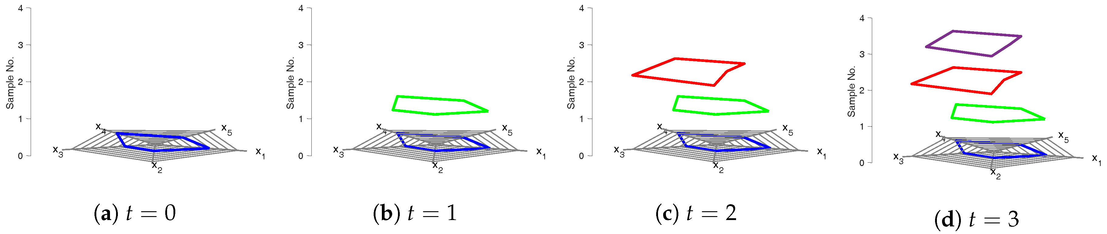
Kiviat diagrams [16] can be considered as an evolution of the parallel coordinates plot described above. In Kiviat diagrams, axes are placed radially around a center point; this differs from both score plots and parallel coordinate plots, where axes are normal and, respectively, parallel to one another. Like parallel coordinate plots, Kiviat diagrams allow for plotting multivariate (normalized and mean-centered) data. However, unlike parallel coordinates, where a multivariate data sample is represented as an open (set of) linear segment(s), a data sample in Kiviat diagrams is presented as a closed (but not necessarily regular or convex) polygon. Using an additional coordinate, normal to the plotting plane, the time dimension can be explicitly captured [17] (Figure 2a).
The result of plotting a multivariate time series dataset in this framework is a three-dimensional figure resembling a cylinder (Figure 2b,c). The two-dimensional polygon of the Kiviat diagram at a given sample time can therefore be considered a “data slice” that corresponds to the same time sample in the time series data. We note that similar three-dimensional Kiviat diagrams have been previously used in computer science for the visualization of software performance [18,19].
2.1. Fault Detection
We begin by examining how fault detection can be conducted in parallel coordinates. Recent research in parallel coordinates has focused on process monitoring and fault detection. Initial efforts [20,21,22] explored plotting the raw variables or leading PCA components (as a form of dimensionality reduction). A common feature of these methods is the use of univariate control limits to define the region of normal operation. Unfortunately, univariate control limits are not amenable to the monitoring of a complex process with many interactions between variables, as demonstrated, e.g., by Kourti and MacGregor [23] (see Figure 3).
Later work by Dunia et al. [24,25], Albazzaz et al. [26] and Gajjar and Palazoglu [27] expanded the set of variables to plot to include PCA-based statistical tests, such as Hotelling’s and the SPE, as well as improved definitions of the confidence regions.
Turning now to the proposed time-explicit Kiviat diagrams, we note that this representation allows for the definition of centroids [13] as the geometric center of a polygon corresponding to a data sample. The centroid locations are computed in a 2D Cartesian coordinate system whose (0,0) point is located at the center of the Kiviat diagram corresponding to each data sample.
For an n-dimensional dataset with m samples, the locations of the n polygon vertices translate to , , and the coordinates of the centroid for data sample can be determined as:
In this way, we are able to represent every polygon, and consequently, every sample, by its corresponding centroid. This allows us to visualize the state of a process as a point (the centroid) and immediately translates into a useful representation to changes in the process: process fluctuations cause variations in sample measurements, which in turn results in a change in the shape of a polygon, which leads to a corresponding change of the centroid positions [13] (Figure 4).
Furthermore, the data are pre-processed using normalization prior to plotting, so the centroids of data collected from a process operating at its nominal steady state will be located near the center of the Kiviat diagram, and any deviation from the center would indicate a deviation in the process.
However, due to noise in process measurements, this ideal “steady state region” is not restricted to a single point in the plot. Therefore, it is necessary to create and visualize a “normal operating region” in Kiviat diagrams to distinguish between normal and abnormal operation of a process.
Due to the different characteristics of the types of processes, the method by which a “normal operation region” is defined varies according to the type of process. In the following sections, we describe the definition of the normal operating region and the associated fault detection approaches for three common types of processes: continuous, batch and periodic. The approaches described below are based on previous work by the authors [13,14,15].
Remark 1.
While the use of principal components guarantees that the data plotted in the Kiviat diagrams are orthogonal, the order of axes remains a factor in the calculation of centroids when plotting physical variables and in the subsequent fault detection activities. The optimal sequencing of variables in the Kiviat diagram remains an area of active research.
3. Applications
3.1. Continuous Processes
For the purpose of the present work, we define a continuous process as a system that operates at or close to a steady state the majority of the time. We note that continuous processes can feature multiple steady states; for simplicity, we consider systems with a single steady state. Moreover, we assume that data are available for this steady state and represent a period of “good” operation, with any deviation of the steady state being the result of the presence of a fault in the system. Thus, our goal is to, (i) statistically define this steady state in our geometric framework and (ii) establish a statistically meaningful fault detection framework on this basis. In our presentation, we follow closely the developments in [13]: using the centroids described above, a confidence region in the shape of an ellipse can be established (the reader is referred to [13] for a complete description of this process); this region defines the nominal “steady state” of the process. The confidence ellipse is computed using the centroids as follows:
- Step 1
- Assume that matrix (which contains m samples of n process variables) represents a period of operation where the steady state process performance is considered to be optimal (a “golden period” [28]). We compute its eigenvalues and eigenvectors , of the data covariance matrix , i.e.,
- Step 2
- Using the and values, we define an n-dimensional confidence ellipsoid around the steady state operating region. The coordinates of the center of the ellipsoid are calculated from:In the n-dimensional hyperspace, the orientation of the axes of the ellipsoid is provided by the eigenvectors , while the length of each axis is determined by the eigenvalues of the covariance matrix. The lengths of the confidence ellipsoid radii are scaled using the critical value of the distribution that corresponds to the desired confidence level of the ellipsoid:
- Step 3
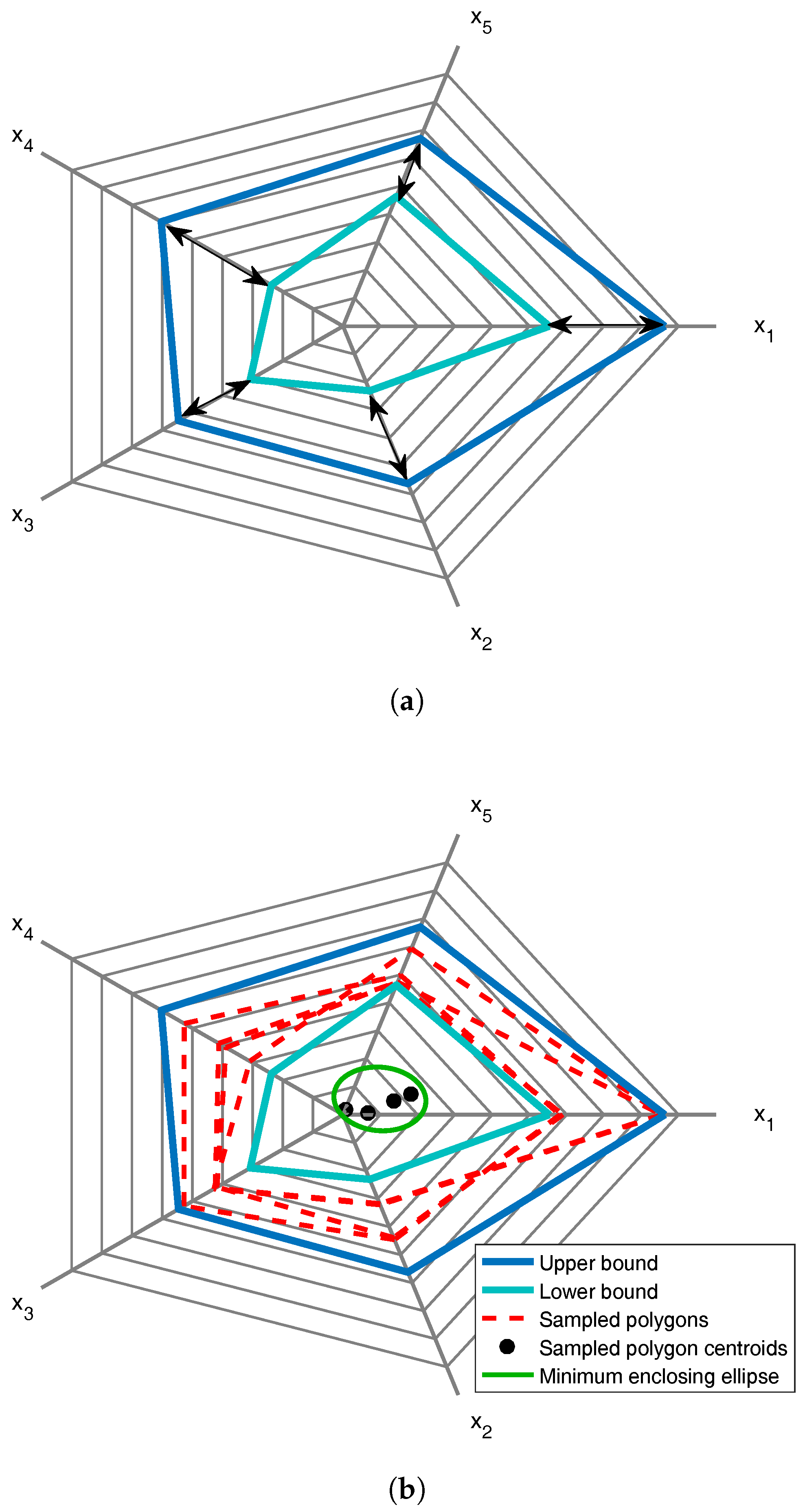
- The extremes of the n-dimensional ellipsoid can be represented on the Kiviat diagram (Figure 5a) via a projection, which then allows us to define an appropriate confidence region for the centroids.
- Step 4
- The annular region between the extremes of the n-dimensional ellipsoid projected on the Kiviat diagram is sampled to generate random data points using values uniformly distributed within the bounds of each variable (Figure 5b).Polygons situated close to the edges of the annular region could in fact lie outside the confidence ellipsoid. To prevent this, each random polygon is verified to correspond to a point inside the confidence ellipsoid in the n-dimensional ellipsoid by reversing the projection from the Kiviat diagram to n-dimensional space. To to so, we follow two simple steps:
- (a)
- Apply the transformation matrix to the coordinates Y of the randomly-generated polygon, to obtain the transformed coordinates Z:where
- (b)
- Compare the norm with the radius of the unit sphere. Then, if , the randomly-generated polygon is indeed associated with a point within the confidence ellipsoid. The polygon is otherwise discarded, and a new polygon is generated.
- Step 5
- The procedure is repeated until the prescribed number of random polygons (typically, 5000) is reached. Then, the calculation of the minimum-area enclosing ellipse [29], of center c, , is an optimization problem formulated as:where P is the matrix of centroid locations.
Fault detection is then performed in the following manner:
- Calculate the corresponding polygon and centroid in the Kiviat diagram for every new data sample.
- Assess if the centroid lies outside of the confidence region.
- Flag the sample as a faulty sample if it lies outside of the confidence region. A separate criterion (e.g., two consecutive samples are identified as faulty) can be implemented to raise a process fault.
To demonstrate its effectiveness, we applied the procedure described above to the Tennessee Eastman Process (TEP) simulator [30]. The Tennessee Eastman Process simulator is a benchmarking tool widely used in process control and monitoring literature involving continuous processes. We used the MATLAB version of the simulation [31] to obtain the data discussed below.
Training data (representing steady state operation of the process) are obtained by running the process simulator for 12 (simulation, rather than “wall clock”) hours. For each fault, the process was simulated for 12 h (720 min) of operation, and faults were imposed at t = 300 min. Random noise was overlaid on the data for every run. Principal component analysis (PCA) was used to reduce the dimensionality of the data; nine principal components were used to capture 70.1% of the variance in the training data. The confidence level used to calculate the confidence ellipse is 95%.
Below, we compare the fault detection delay (amount of time required to detect the fault after it has been introduced) of our method against regular PCA T and Q, as well as dynamic PCA T and Q metrics. As an added challenge, we choose combinations of faults as our test cases, noting that in our previous work, we only consider individual faults. The choice of multiple fault events was made taking care to avoid (based on our physical judgment) simultaneously imposing errors that would “cancel each other out.” The list of relevant faults is presented in Table 1, while the fault detection results are shown in the sequel.
The results in Table 2 show that our proposed method is comparable to other methods in terms of fault detection delay. We also examined the missed detection and false detection rates (in Table 3 and Table 4 respectively) of the different methods using the definition proposed by Zhang [33]. Zhang defines “false detection” as data that fall outside of the defined confidence level (95%) before the fault has occurred and “missed detection” as data that fall inside of the defined confidence level (95%) after the fault has occurred.
3.2. Batch Processes
Batch processes differ fundamentally from continuous ones in that they never reach a steady state. A batch is defined in terms of a starting point and and end point, with the state of the process changing continuously between the two. Thus, an alternate method is proposed for defining confidence regions in 3D Kiviat diagrams for batch systems. The presentation below follows closely the developments in [14].
Specifically, we propose the use of multiple confidence regions, such that the entire trajectory of the batch is captured, describing the expected “normal” performance of the process at each time point in the course of the batch. To this end, batch data (with dimensions I batches samples variables) are unfolded into a two-dimensional array using time-wise unfolding, as seen in Figure 6. As in the case of continuous processes, we assume that multiple datasets corresponding to several “good” batches are available as training data. Each training batch is plotted on the same radial plot, and the centroids for every sample in the batch are computed. The centroids for the same sample time, but for multiple batches are used to compute a confidence region specifically for that sample time (i.e., all samples at are used to calculate the confidence region for ), using the procedure described above for continuous processes.
The confidence ellipses are stacked (similar to the way polygons in Kiviat diagrams can be stacked) to allow for better visualization of the trajectory of the batch, as seen in Figure 7. Fault detection is performed by comparing the centroids of new batch samples against the confidence regions at each sample time.
This mechanism can identify the moment in time at which a fault occurs in a batch run, enabling operators to diagnose potential issues in the batch process; the mechanism can be used both in real time, as well as an analysis tool after the completion of the batch.
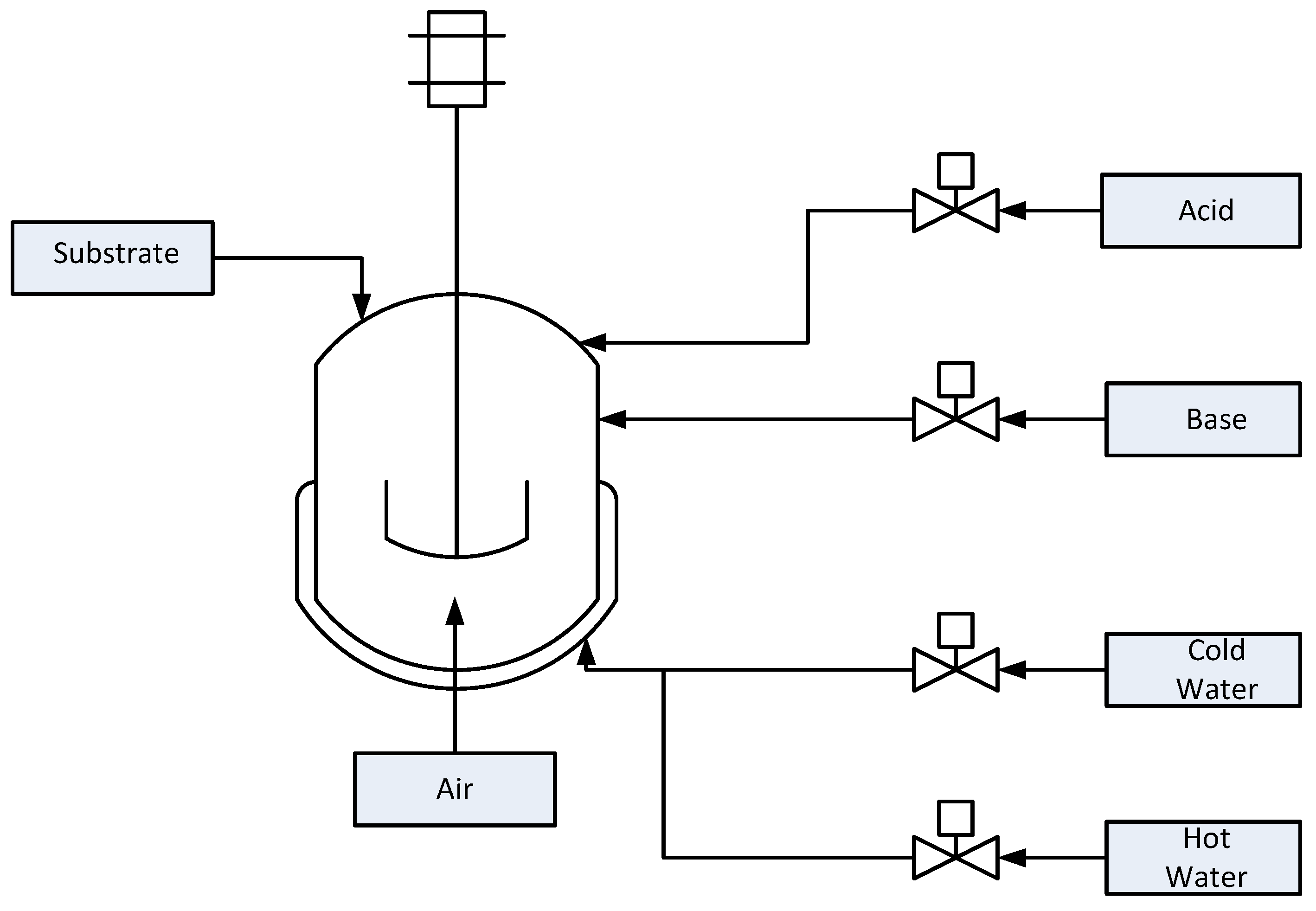
To demonstrate this fault detection mechanism, we use the PenSim [34] bioreactor simulator. The fault detection performance is compared against conventional multiway PCA (MPCA) T and Q statistics [5] as described below. A schematic of the process is provided in Figure 8.
The input variables are the aeration rate, agitator power and glucose feed rate. The model predicts the concentrations of biomass, glucose, penicillin, dissolved oxygen and carbon dioxide. Culture volume, acid flow rate, base flow rate, reactor temperature, generated heat, pH value and cooling/heating water flow rate are also computed in the simulation [34]. Sixteen process variables (listed in Table 5) are assumed to be measured and used for data-driven process monitoring and fault detection. Two control loops are used to maintain the temperature and pH of the reactor. Nine faults (Table 6) can be imposed, consisting of step/ramp changes in the inputs.
For this case study, a set of twenty batches run normally are used as a “reference” of good performance and used to establish the sample-wise confidence ellipses. Subsequent simulations are run with the faults specified in Table 6, occurring at t = 100 h and lasting till t = 130 h. We implemented the fault detection methodology described above, along with online multiway PCA (MPCA) [5] for comparison purposes.
Table 7 shows a comparison of the fault detection speeds, and Table 8 presents the false detection rates (defined as normal data samples being flagged as faulty before a fault occurs) for the visualization-based and MPCA-based methods.
The data presented above demonstrate that the proposed framework allows for detecting faults occurring in batch processes at a speed comparable to that of MPCA, while reducing the number of false alarms raised. Our approach also offers an intuitive way for visualizing batch data, either in real time or as a post-operational analysis.
3.3. Periodic Processes
As a third class of chemical processes, we consider systems under periodic operation. The operation of such processes consists of cycles whose beginning and end points in the state space typically coincide during normal operation. Their steady state is cyclical, rather than point-wise (as the case of continuous processes). While such systems are, strictly speaking, neither batch nor continuous, a number of interesting parallels can be drawn between the system classes considered in this paper:
- Periodic processes resemble to some extent batch processes, in that each cycle can be considered to be a “batch.” Thus, “normal” operation can be defined in terms of repeatability, with all such “batches” being the same in a statistical sense. Note, however, that during normal operation, each cycle typically begins and ends in the same state; this is not the case for batch systems, where the start and end point are typically very different.
- The observation above hints at a potential similarity between periodic processes and continuous processes; a periodic process can be construed as “continuous” in the sense that it is desired that the cycles be reproducible and each cycle be statistically the same as its predecessor.
These similarities allowed us to develop [15] a fault detection mechanism for periodic processes that relies on the concepts presented above for continuous and batch processes. Specifically, we divide the fault detection activity into two steps: a inter-cycle fault detection step that uses the oscillatory steady state to identify problematic cycles and an intra-cycle fault detection step that identifies where in the problematic cycles the deviation occurs.
In the inter-cycle step, we define a feature called the cyclic centroid [15] that characterizes a full cycle of the process in the aggregate. Since there are multiple cycles in the process, multiple cyclic centroids are obtained from the data. By then defining a confidence ellipse around cyclic centroids corresponding to the cycles of normal operation, we are able to identify problematic cycles by monitoring the cyclic centroids. We note that this step is very similar to the fault detection approach proposed earlier for continuous processes.
The following, intra-cycle step seeks to identify exactly when in the cycle the problem or fault has occurred. This is done by defining confidence ellipses for every sample across cycles of normal operation; this creates a cycle trajectory that corresponds to the dynamics of a normal operating cycle. By comparing the samples of a problematic cycle against the corresponding sample confidence ellipse, the moment when deviation begins to occur in the problematic cycle can be identified, as seen in Figure 9. This step is based on the principles for fault detection in batch systems, outlined above.
This two-step method is applied on an air separation system, aimed at separating oxygen from air via pressure swing adsorption (PSA). As a high purity oxygen product is desired for an air separation system, being able to detect faults quickly is important to prevent penalties associated with delivering off-spec products.
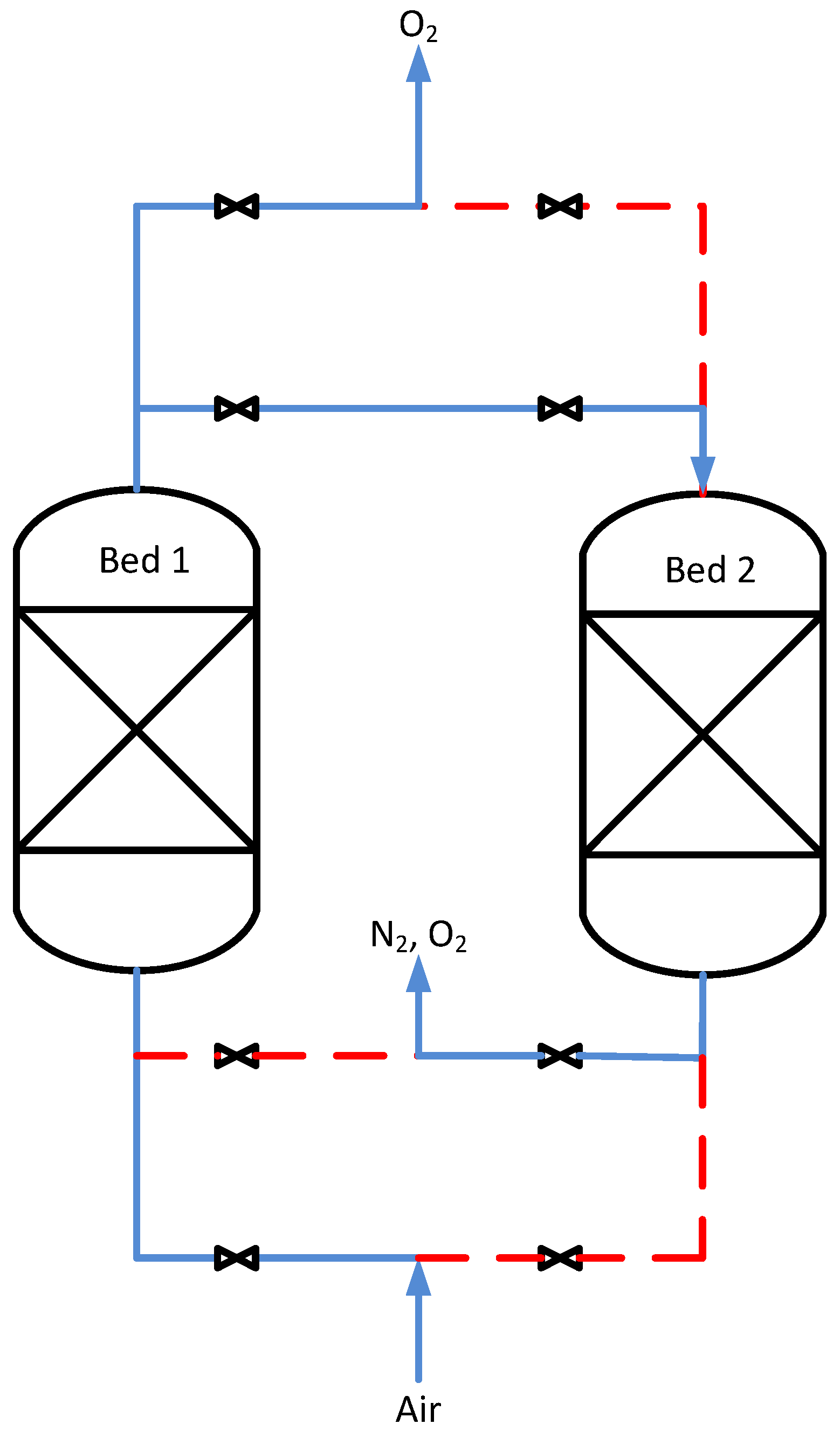
The PSA system was simulated using the gPROMS gML Separations-Adsorption model library [35]. The model represents a two-bed, four-step isothermal process (Figure 10), whose periodic operation follows the switching strategy described in Table 9.
The parameters for the PSA model (the model captures radial and axial transport, as well as the reactions in the beds) are provided in Table 10.
A total of 26 variables relating to the flow rate of the feed, as well as pressures and concentrations in and across both beds were used for observation. White noise with a signal-to-noise ratio of 30 was added to the simulated data. The observed period of a single cycle is 150 s.
The temperature and pressure of the feed flow into the beds were modified to simulate faults in the process. These faults were implemented at t = 5000 s, and the process ran for 10,000 s total. Similar to the previous case studies, the detection delay is the metric used to evaluate fault detection performance.
Due to the dearth of research regarding fault detection in periodic processes, two conventional methods of fault detection used in continuous and batch processes were adapted for our purposes. The two methods selected were dynamic principal component analysis (DPCA) and multiway principal component analysis (MPCA). MPCA, as described above, is a PCA model used when dealing with batch data, and DPCA is a locally updating PCA model used for continuous datasets. For MPCA, each cycle is treated as one batch run in the data, while for DPCA, the moving window size used is set to the observed period of the data; this means that the model would be updated after every cycle.
As seen from Table 11, our method performs better than the adapted methods for the majority of the cases. The two adapted PCA-based methods perform comparably to one another.
4. Conclusions
In this paper, we provide an overview of recently-developed visualization techniques for process data. The concept underpinning these techniques is a time-explicit Kiviat diagram, which allows for plotting multivariate time series data collected during the operation of chemical processes. On this cornerstone, we developed specific visualization and fault detection techniques for three major classes of chemical processes: continuous, batch and periodic. On the visualization front, these techniques allow for plotting and presenting large amounts of data on a unified plot. Furthermore, using simulation case studies, we compared the fault detection performance of the proposed methods with that of conventional methods used in the literature and in practice. Of particular interest is the application of these ideas to carrying out fault detection for periodic processes, where the available literature is rather scarce in spite of the relatively widespread practical use of such systems, especially in the separations realm.
Author Contributions
Michael Baldea and Thomas F. Edgar formulated and directed the research project. Michael Baldea, Thomas F. Edgar and Ray C. Wang developed the fault detection algorithms, and Ray C. Wang implemented them computationally. Ray C. Wang, Michael Baldea and Thomas F. Edgar analyzed the results and wrote the paper.
Conflicts of Interest
The authors declare no conflict of interest. The funding sponsors had no role in the design of the study; in the collection, analyses, or interpretation of data; in the writing of the manuscript, and in the decision to publish the results.
References
- Venkatasubramanian, V. Drowning in data: Informatics and modeling challenges in a data-rich networked world. AIChE J. 2009, 55, 2–8. [Google Scholar] [CrossRef]
- Venkatasubramanian, V.; Rengaswamy, R.; Yin, K.; Kavuri, S.N. A review of process fault detection and diagnosis: Part I: Quantitative model-based methods. Comput. Chem. Eng. 2003, 27, 293–311. [Google Scholar] [CrossRef]
- Russell, E.L.; Chiang, L.H.; Braatz, R.D. Fault detection in industrial processes using canonical variate analysis and dynamic principal component analysis. Chemom. Intell. Lab. Syst. 2000, 51, 81–93. [Google Scholar] [CrossRef]
- Lee, J.; Yoo, C.K.; Lee, I. Fault detection of batch processes using multiway kernel principal component analysis. Comput. Chem. Eng. 2004, 28, 1837–1847. [Google Scholar] [CrossRef]
- Lee, J.; Yoo, C.K.; Lee, I. Enhanced process monitoring of fed-batch penicillin cultivation using time-varying and multivariate statistical analysis. J. Biotechnol. 2004, 110, 119–136. [Google Scholar] [CrossRef] [PubMed]
- Lee, J.; Yoo, C.; Lee, I. Statistical process monitoring with independent component analysis. J. Proc. Contr. 2004, 14, 467–485. [Google Scholar] [CrossRef]
- He, Q.P.; Wang, J. Statistics pattern analysis: A new process monitoring framework and its application to semiconductor batch processes. AIChE J. 2011, 57, 107–121. [Google Scholar] [CrossRef]
- Kano, M.; Nagao, K.; Hasebe, S.; Hashimoto, I.; Ohno, H.; Strauss, R. Comparison of multivariate statistical process monitoring methods with applications to the Eastman challenge problem. Comput. Chem. Eng. 2002, 26, 161–174. [Google Scholar] [CrossRef]
- Yoon, S.; MacGregor, J.F. Fault diagnosis with multivariate statistical models part I: Using steady state fault signatures. J. Proc. Contr. 2001, 11, 387–400. [Google Scholar] [CrossRef]
- Venkatasubramanian, V.; Rengaswamy, R.; Yin, K.; Kavuri, S.N. A review of process fault detection and diagnosis: Part III: Process history based methods. Comput. Chem. Eng. 2003, 27, 324–346. [Google Scholar] [CrossRef]
- Qin, S.J. Survey on data-driven industrial process monitoring and diagnosis. Annu. Rev. Control 2012, 36, 220–234. [Google Scholar] [CrossRef]
- Inselberg, A. Parallel Coordinates; Springer: New York, NY, USA, 2009. [Google Scholar]
- Wang, R.; Edgar, T.F.; Baldea, M.; Nixon, M.; Wojsznis, W.; Dunia, R. Process Fault Detection Using Time-Explicit Kiviat Diagrams. AICHE J. 2015, 61, 4277–4293. [Google Scholar] [CrossRef]
- Wang, R.; Edgar, T.F.; Baldea, M.; Nixon, M.; Wojsznis, W.; Dunia, R. A Geometric Framework for Batch Data Visualization, Process Monitoring and Fault Detection. J. Process Control 2017. accepted. [Google Scholar]
- Wang, R.; Edgar, T.F.; Baldea, M. A geometric framework for monitoring and fault detection for periodic processes. AIChE J. 2017, 63, 2719–2730. [Google Scholar] [CrossRef]
- Kolence, K.W. The software empiricist. ACM SIGMETRICS Perform. Eval. Rev. 1973, 2, 31–36. [Google Scholar] [CrossRef]
- Tominski, C.; Abello, J.; Schumann, H. Interactive poster: 3D axes-based visualizations for time series data. In Proceedings of the IEEE Symposium on Information Visualization 2005 (InfoVis 2005), Minneapolis, MN, USA, 23–25 October 2005. [Google Scholar]
- Hackstadt, S.T.; Malony, A.D. Visualizing parallel programs and performance. IEEE Comput. Graph. Appl. 1995, 15, 12–14. [Google Scholar] [CrossRef]
- Fanea, E.; Carpendale, S.; Isenberg, T. An interactive 3d integration of parallel coordinates and star glyphs. In Proceedings of the IEEE Symposium on Information Visualization 2005 (InfoVis 2005), Minneapolis, MN, USA, 23–25 October 2005; pp. 149–156. [Google Scholar]
- Albazzaz, H.; Wang, X.Z. Historical data analysis based on plots of independent and parallel coordinates and statistical control limits. J. Proc. Contr. 2006, 16, 103–114. [Google Scholar] [CrossRef]
- Wang, X.; Medasani, S.; Marhoon, F.; Albazzaz, H. Multidimensional visualization of principal component scores for process historical data analysis. IECres 2004, 43, 7036–7048. [Google Scholar] [CrossRef]
- He, Q.P. Multivariate visualization techniques in statistical process monitoring and their applications to semiconductor manufacturing. In Proceedings of the SPIE 31st International Symposium on Advanced Lithography, San Jose, CA, USA, 19 February 2006; p. 615506. [Google Scholar]
- MacGregor, J.F.; Kourti, T. Statistical process control of multivariate processes. Contr. Eng. Prac. 1995, 3, 403–414. [Google Scholar] [CrossRef]
- Dunia, R.; Rochelle, G.; Edgar, T.F.; Nixon, M. Multivariate Monitoring of a Carbon Dioxide Removal Process. Comput. Chem. Eng. 2014, 60, 381–395. [Google Scholar] [CrossRef]
- Dunia, R.; Edgar, T.F.; Nixon, M. Process monitoring using principal components in parallel coordinates. AIChE J. 2013, 59, 445–456. [Google Scholar] [CrossRef]
- Albazzaz, H.; Wang, X.Z.; Marhoon, F. Multidimensional visualisation for process historical data analysis: A comparative study with multivariate statistical process control. J. Process Control 2005, 15, 285–294. [Google Scholar] [CrossRef]
- Gajjar, S.; Palazoglu, A. A data-driven multidimensional visualization technique for process fault detection and diagnosis. Chemom. Intell. Lab. Syst. 2016, 154, 122–136. [Google Scholar] [CrossRef]
- Yu, J.; Qin, S.J. Statistical MIMO controller performance monitoring. Part I: Data-driven covariance benchmark. J. Proc. Contr. 2008, 18, 277–296. [Google Scholar] [CrossRef]
- Moshtagh, N. Minimum volume enclosing ellipsoid. Convex Optim. 2005, 111, 112. [Google Scholar]
- Downs, J.; Vogel, E. A plant-wide industrial process control problem. Comput. Chem. Eng. 1993, 17, 245–255. [Google Scholar] [CrossRef]
- Ricker, N.L. Tennessee Eastman Challenge Archive. Available online: http://depts.washington.edu/control/LARRY/TE/download.html (accessed on 15 April 2017).
- Lee, J.; Yoo, C.; Lee, I. Statistical monitoring of dynamic processes based on dynamic independent component analysis. Chem. Eng. Sci. 2004, 59, 2995–3006. [Google Scholar] [CrossRef]
- Zhang, Y. Fault Detection and Diagnosis of Nonlinear Processes Using Improved Kernel Independent Component Analysis (KICA) and Support Vector Machine (SVM). Ind. Eng. Chem. Res. 2008, 47, 6961–6971. [Google Scholar] [CrossRef]
- Birol, G.; Ündey, C.; Cinar, A. A modular simulation package for fed-batch fermentation: Penicillin production. Comput. Chem. Eng. 2002, 26, 1553–1565. [Google Scholar] [CrossRef]
- Process Systems Enterprise, gPPROMS gML Separations—Adsoprtion Model Library. Available online: www.psenterprise.com/gproms (accessed on 30 April 2017).
Figure 1.
Data visualization in parallel coordinates for a five-dimensional dataset. Each coordinate can be regarded as the ordinate of a regular time series plot. Data samples are added to the plot as they are acquired, in the form of a set of linear segments. As time progresses (a–d), current data are typically shown along with previously-plotted information to capture trends.
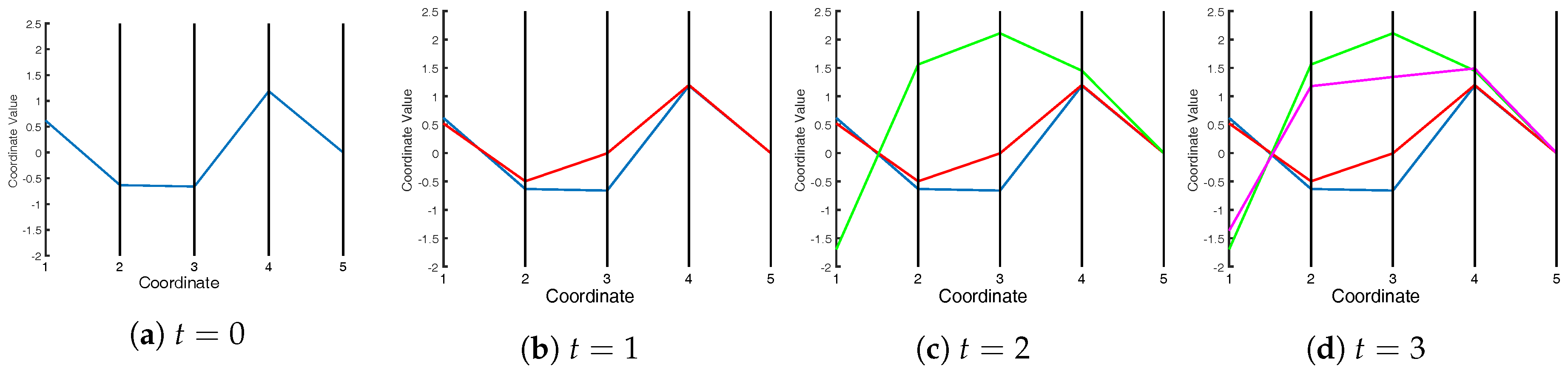
Figure 2.
Representing multi-dimensional time series data using Kiviat diagrams. The same five-dimensional dataset as in Figure 1, with one-minute sampling time, is used for illustration purposes. The first sample is plotted (a) on the Kiviat plot having a time axis that is normal to the plot plane. The next samples are added as additional Kiviat plots whose planes are parallel to the plane of the first and spaced along the time axis according to the sampling time (b–d). The diagram can be updated by adding such “data slices” in a first-in, first-out manner.

Figure 3.
Univariate control limits suffer from “blind spots” in a multivariate setting: a data sample (marked in red) can be within the control limits from the perspective of every variable on the respective univariate control charts, but fall outside the multivariate confidence region. LCL and UCL represent univariate lower and upper control limits, respectively.
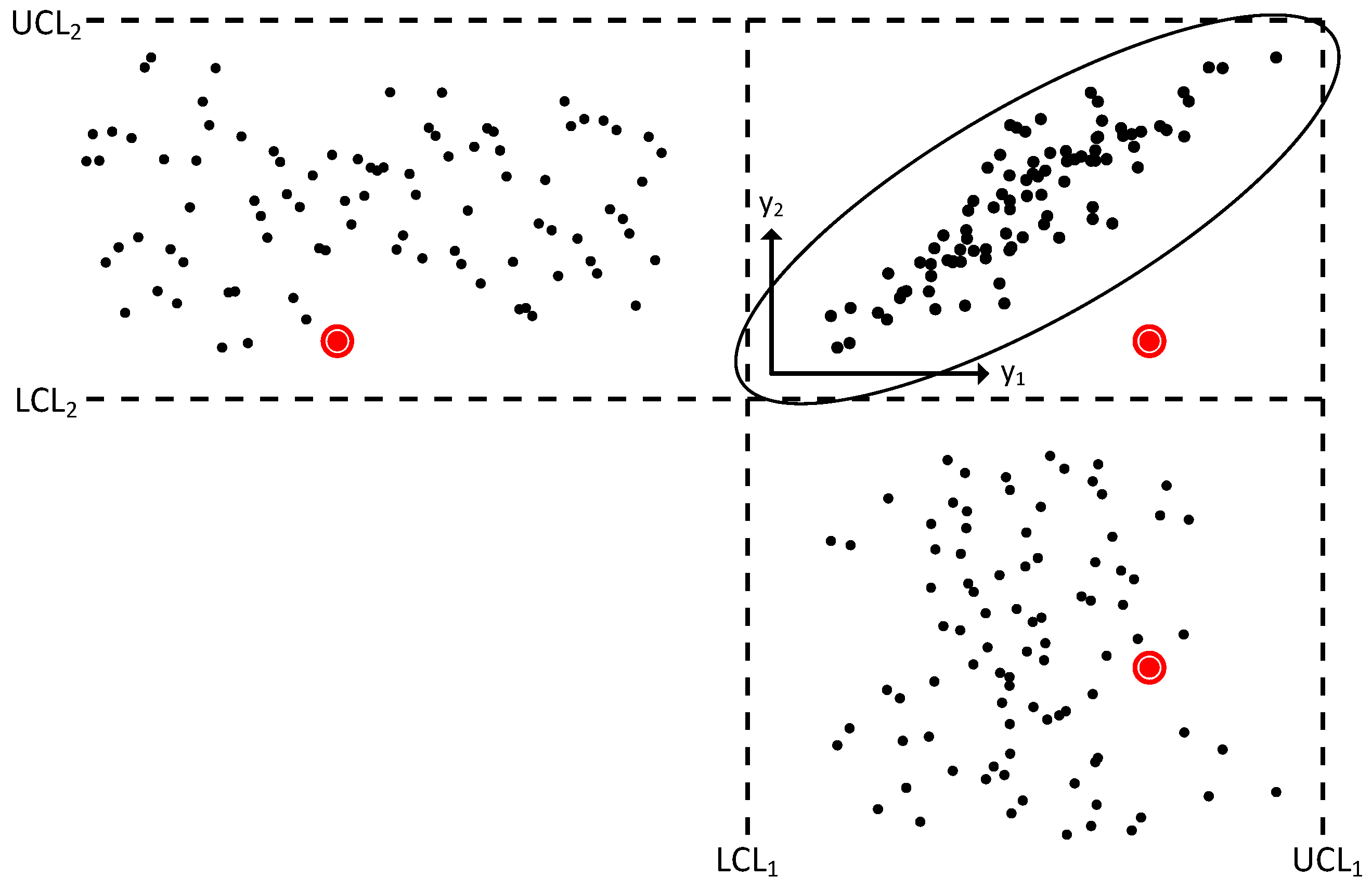
Figure 4.
The centroid of each slice constitutes a single-point, multivariate representation of each data slice. (b) is a “top-down” view of (a), with the centroids shown as diamonds.
Figure 4.
The centroid of each slice constitutes a single-point, multivariate representation of each data slice. (b) is a “top-down” view of (a), with the centroids shown as diamonds.
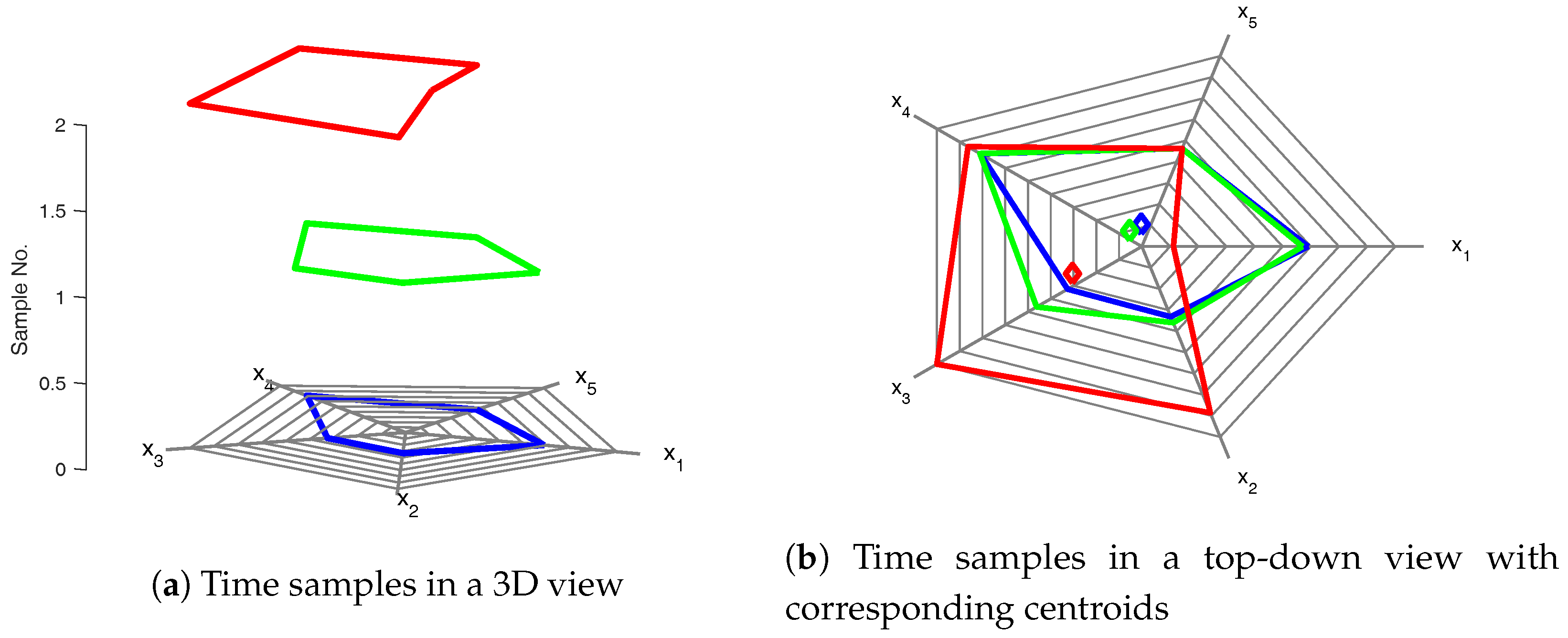
Figure 5.
(a) Limits in time-resolved Kiviat diagram. Black arrows indicate limits for each variable. Blue and green lines are the extrema of the confidence ellipsoid. (b) Sampled points within the annular region (in red) are used to generate the confidence ellipse.
Figure 5.
(a) Limits in time-resolved Kiviat diagram. Black arrows indicate limits for each variable. Blue and green lines are the extrema of the confidence ellipsoid. (b) Sampled points within the annular region (in red) are used to generate the confidence ellipse.

Figure 6.
Unfolding of batch data. (a) Batch data in three dimensions; (b) batch-wise unfolding; (c) time-wise unfolding.
Figure 6.
Unfolding of batch data. (a) Batch data in three dimensions; (b) batch-wise unfolding; (c) time-wise unfolding.
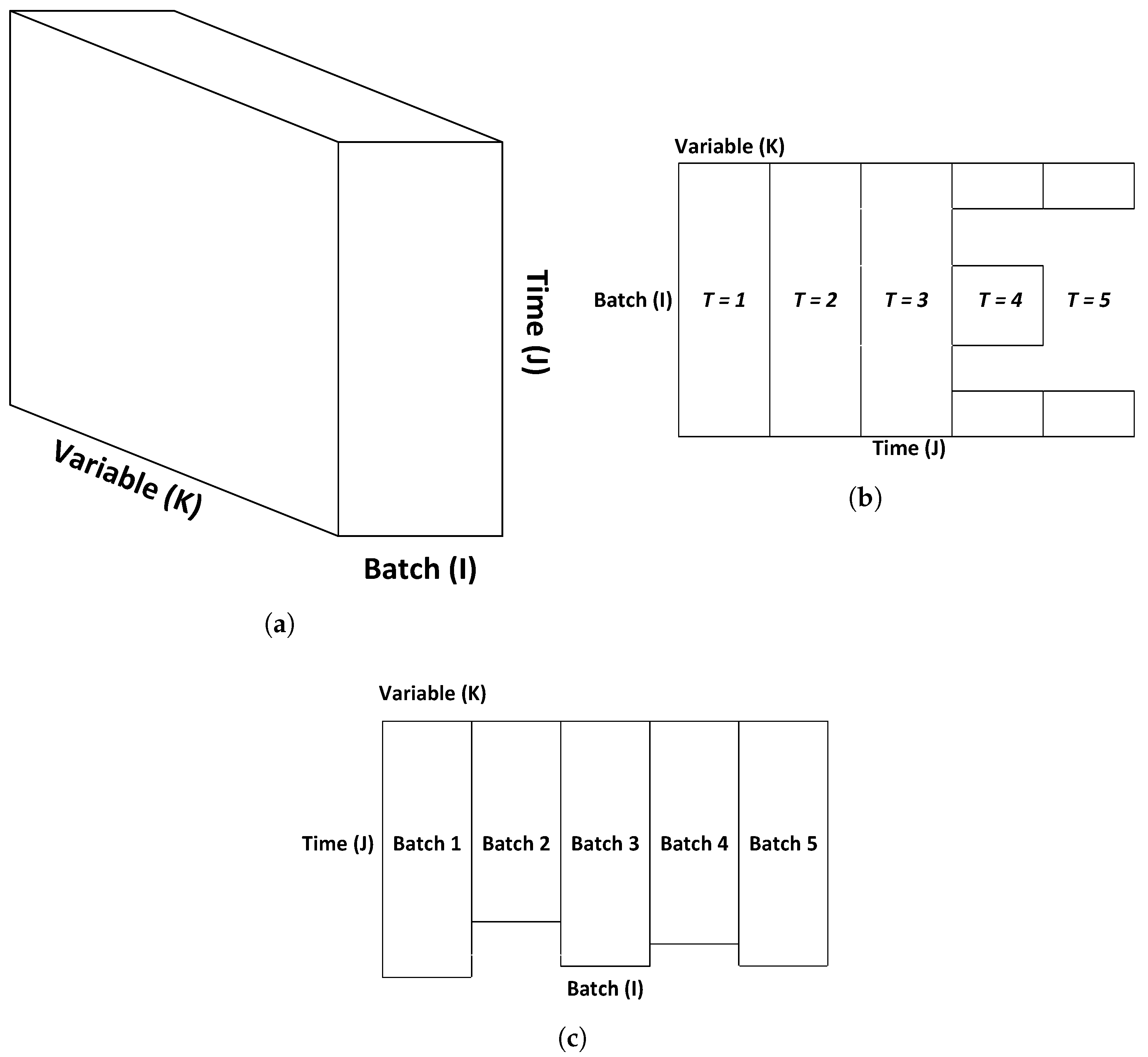
Figure 7.
The confidence region at every data point drawn (green) for an illustrative batch process data set resembles a funnel or tube in 3D.
Figure 7.
The confidence region at every data point drawn (green) for an illustrative batch process data set resembles a funnel or tube in 3D.
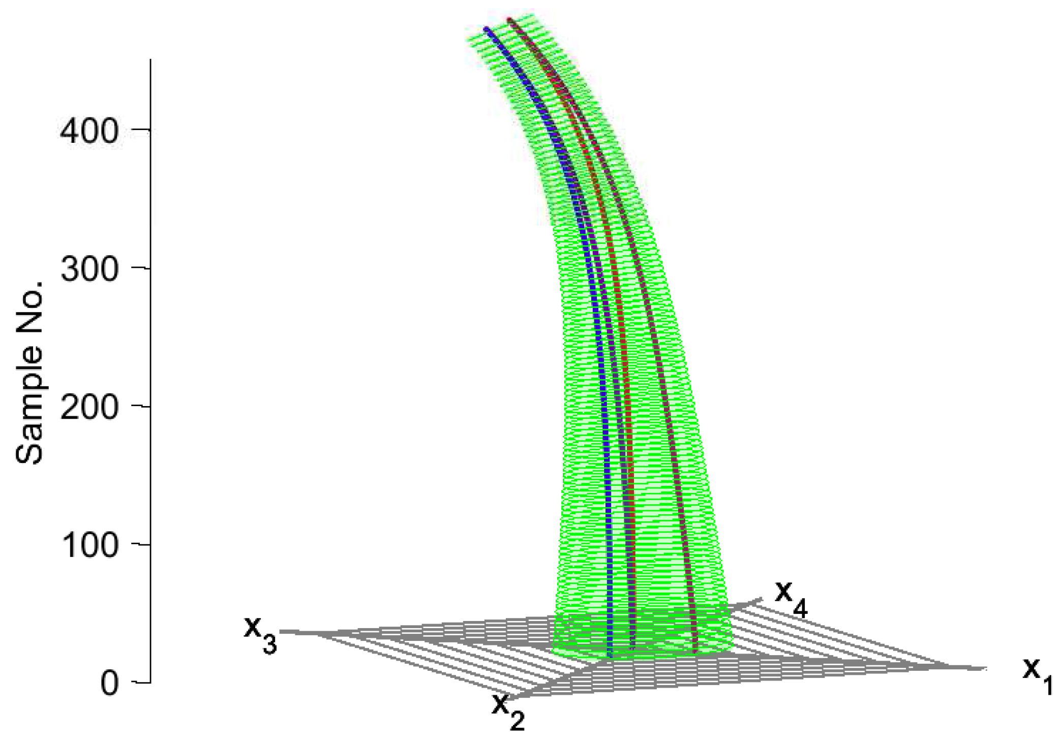
Figure 8.
Schematic of the the PenSim process, reproduced with permission from [34]. Copyright Elsevier, 2002.
Figure 8.
Schematic of the the PenSim process, reproduced with permission from [34]. Copyright Elsevier, 2002.

Figure 9.
Intra-cycle fault detection is carried out on a problematic cycle. Each sample in the problematic cycle is compared against the intra-cycle confidence region (in red); samples that lie inside the region are colored in blue, whereas samples that lie outside the confidence region are colored in black.
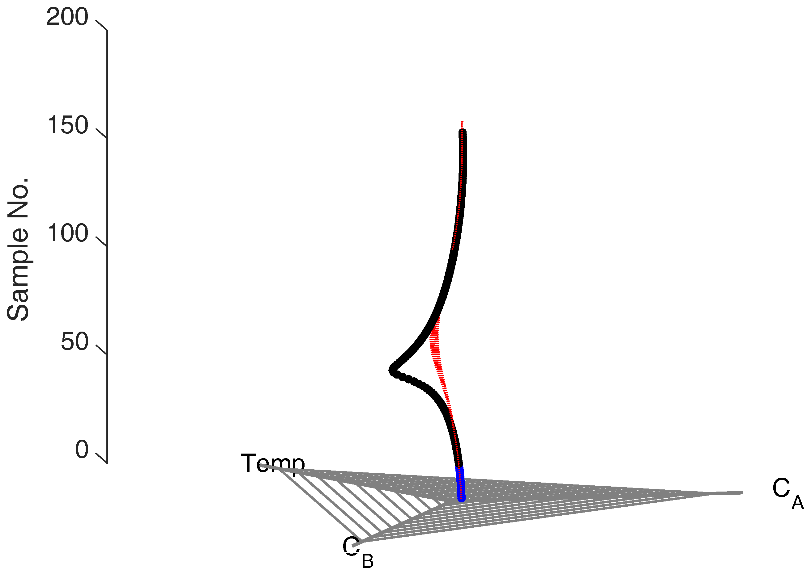
Figure 10.
Schematic of the PSA system; the solid lines denote the flow pathway of the gas, while the dashed lines represent inactive piping in the cycle. As shown in the figure, Bed 1 is the active bed (flow denoted in blue), while Bed 2 is being regenerated.
Figure 10.
Schematic of the PSA system; the solid lines denote the flow pathway of the gas, while the dashed lines represent inactive piping in the cycle. As shown in the figure, Bed 1 is the active bed (flow denoted in blue), while Bed 2 is being regenerated.


Table 1.
Faults that can be implemented in Tennessee Eastman Process simulator, reproduced with permission from [32]. Copyright Elsevier, 2004.
Table 1.
Faults that can be implemented in Tennessee Eastman Process simulator, reproduced with permission from [32]. Copyright Elsevier, 2004.
| Fault No. | Description | Type |
|---|---|---|
| 1 | A/C feed ratio, B Composition constant (Stream 4) | Step |
| 2 | B Composition, A/C ratio constant (Stream 4) | Step |
| 3 | D feed temperature (Stream 2) | Step |
| 4 | Reactor cooling water inlet temperature | Step |
| 5 | Condenser cooling water inlet temperature | Step |
| 8 | A, B, C feed composition (Stream 4) | Random variation |
| 10 | C feed temperature (Stream 4) | Random variation |
| 14 | Reactor cooling water valve | Sticking |
Table 2.
Fault detection delay for the Tennessee Eastman Process.
| Fault Detection Delay (Minutes) (Lower Is Better) | |||||
|---|---|---|---|---|---|
| Fault Numbers | Proposed Method | PCA T | PCA Q | DPCA T | DPCA Q |
| 1 | 3 | 3 | 9 | ||
| 3 | 17 | 2 | 6 | 6 | |
| 1 and 3 | 3 | 3 | 9 | ||
| 2 | 8 | 6 | 91 | 24 | 94 |
| 4 | 2 | 6 | 138 | 2 | 94 |
| 2 and 4 | 2 | 2 | 104 | 6 | 107 |
| 5 | 2 | 2 | 145 | 3 | 131 |
| 10 | 52 | 41 | 106 | 47 | 117 |
| 5 and 10 | 2 | 2 | 3 | ||
| 8 | 46 | 21 | 116 | 65 | 119 |
| 14 | 8 | 3 | 8 | ||
| 8 and 14 | 4 | 2 | 113 | 6 | 119 |
Blank cells indicate that no fault was detected.
Table 3.
Missed detection rates for the Tennessee Eastman Process.
| Missed Detection Rates (Lower Is Better) | |||||
|---|---|---|---|---|---|
| Fault Numbers | Proposed Method | PCA T | PCA Q | DPCA T | DPCA Q |
| 1 | 0.0179 | 0.0179 | 0.0714 | ||
| 3 | 0.542 | 0.0095 | 0.9786 | ||
| 1 and 3 | 0.0174 | 0.0174 | 0.0696 | ||
| 2 | 0.018 | 0.0103 | 0.9205 | 0.059 | 0.9282 |
| 4 | 0.040 | 0.0024 | 0.9786 | 0.399 | 0.9406 |
| 2 and 4 | 0.0124 | 0.0025 | 0.9208 | 0.0025 | 0.9282 |
| 5 | 0.002 | 0.0024 | 0.981 | 0.0356 | 0.9477 |
| 10 | 0.138 | 0.095 | 0.9287 | 0.1093 | 0.9145 |
| 5 and 10 | 0.0024 | 0.0024 | 0.0048 | ||
| 8 | 0.102 | 0.0784 | 0.9121 | 0.152 | 0.9192 |
| 14 | 0.040 | 0.0048 | 0.0166 | ||
| 8 and 14 | 0.0261 | 0.0024 | 0.905 | 0.0119 | 0.9192 |
Blank cells indicate that no fault was detected.
Table 4.
False detection rates for the Tennessee Eastman Process.
| False Detection Rates (Lower Is Better) | |||||
|---|---|---|---|---|---|
| Fault Numbers | Proposed Method | PCA T | PCA Q | DPCA T | DPCA Q |
| 1 | 0.0267 | 0.0533 | 0 | ||
| 3 | 0.03 | 0.03 | 0.0133 | ||
| 1 and 3 | 0.0033 | 0.0533 | 0 | ||
| 2 | 0.03 | 0.04 | 0 | 0 | 0 |
| 4 | 0.0367 | 0.05 | 0.0167 | 0 | 0 |
| 2 and 4 | 0 | 0.04 | 0 | 0 | 0 |
| 5 | 0.0367 | 0.0333 | 0.02 | 0 | 0 |
| 10 | 0.04 | 0.0333 | 0 | 0 | 0 |
| 5 and 10 | 0 | 0.03 | 0 | ||
| 8 | 0.0333 | 0.06 | 0 | 0 | 0 |
| 14 | 0.0267 | 0.0467 | 0 | ||
| 8 and 14 | 0.0033 | 0.05 | 0 | 0 | 0 |
Blank cells indicate that no fault was detected.
Table 5.
List of process variables, reproduced with permission from [34]. Copyright Elsevier, 2002.
Table 5.
List of process variables, reproduced with permission from [34]. Copyright Elsevier, 2002.
| Variable Number | Variable Description |
|---|---|
| x | Aeration rate (L/h) |
| x | Agitator power (W) |
| x | Substrate feed rate (L/h) |
| x | Substrate temperature (K) |
| x | Substrate concentration (g/L) |
| x | Dissolved oxygen concentration (g/L) |
| x | Biomass concentration (g/L) |
| x | Penicillin concentration (g/L) |
| x | Culture volume (L) |
| x | Carbon dioxide concentration (g/L) |
| x | pH |
| x | Temperature (K) |
| x | Generated heat (cal) |
| x | Acid flow rate (mL/h) |
| x | Base flow rate (mL/h) |
| x | Cooling/heating water flow rate (L/h) |
Table 6.
Faults simulated by PenSim.
| Fault No. | Description | Type |
|---|---|---|
| 1 | 10% increase in aeration rate | Step |
| 2 | 20% increase in aeration rate | Step |
| 3 | 1.5 L h increase in aeration rate | Ramp |
| 4 | 20% increase in agitation power | Step |
| 5 | 40% increase in agitation power | Step |
| 6 | 0.015 W increase in agitator power | Ramp |
| 7 | 20% increase in substrate feed | Step |
| 8 | 40% increase in substrate feed | Step |
| 9 | 0.12 L h increase in substrate feed | Ramp |
Table 7.
Fault detection delay for the PenSim data. MPCA, multiway PCA.
| Fault Detection Delay (Hours) (Lower Is Better) | |||
|---|---|---|---|
| Dataset # | Proposed Method | MPCA T | MPCA Q |
| 1 | 0.5 | 4 | 3.5 |
| 2 | 0.5 | 9.5 | 9.5 |
| 3 | 13 | 13 | 13 |
| 4 | 1.5 | 2.5 | 3 |
| 5 | 9 | 7 | 7.5 |
| 6 | 15.5 | 11.5 | 12.5 |
| 7 | 20 | 1.5 | 2 |
| 8 | 14.5 | 6 | |
| 9 | 12.5 | 10.5 | |
Blank cells indicate that no fault was detected.
Table 8.
False detection rates for the PenSim data.
| False Detection Rates (Lower Is Better) | |||
|---|---|---|---|
| Dataset # | Proposed Method | MPCA T | MPCA Q |
| 1 | 0.11 | 0.075 | 0.1 |
| 2 | 0.025 | 0.07 | 0.085 |
| 3 | 0.01 | 0.095 | 0.07 |
| 4 | 0.03 | 0.105 | 0.07 |
| 5 | 0.16 | 0.11 | 0.07 |
| 6 | 0 | 0.105 | 0.035 |
| 7 | 0.07 | 0.105 | 0.02 |
| 8 | 0.085 | 0.105 | |
| 9 | 0.07 | 0.105 | |
Blank cells indicate that no fault was detected.
Table 9.
Switching strategy for the pressure swing adsorption (PSA) process.
| Duration (s) | Bed 1 State | Bed 2 State |
|---|---|---|
| 2 | Pressurization | Blowdown |
| 60 | Adsorption | Desorption |
| 2 | Pressure Equalization | Pressure Equalization |
| 2 | Blowdown | Pressurization |
| 60 | Desorption | Adsorption |
| 2 | Pressure Equalization | Pressure Equalization |
Table 10.
Parameters for the PSA model.
| Parameter | Parameter Value |
|---|---|
| Feed flow rate | 0.00364 mol/s |
| Temperature of feed | 298.15 K |
| Length of bed | 0.35 m |
| Radius of bed | 0.0175 m |
| Particle radius | 0.003175 m |
| (void fraction) | 0.4 |
| 300,000 Pa |
Table 11.
Fault detection delay for the PSA system data.
| Fault Detection Delay (Seconds) (Lower is Better) | ||||||
|---|---|---|---|---|---|---|
| Case | Fault Description | Proposed Method | DPCA [3] | DPCA [3] Q | MPCA [5] | MPCA [5] Q |
| 1 | Increased temperature feed by | 89 | 120 | 115 | 118 | 74 |
| 5K in Bed 1 and Bed 2 | ||||||
| 2 | Decreased temperature feed by | 99 | 51 | 54 | 116 | 54 |
| 5K in Bed 1 and Bed 2 | ||||||
| 3 | Pressure drop in Bed 1 by 10% | 59 | 52 | 103 | 118 | 116 |
| 4 | Pressure rise in Bed 2 by 10% | 61 | 122 | 116 | 116 | 173 |
© 2017 by the authors. Licensee MDPI, Basel, Switzerland. This article is an open access article distributed under the terms and conditions of the Creative Commons Attribution (CC BY) license (http://creativecommons.org/licenses/by/4.0/).
Share and Cite
MDPI and ACS Style
Wang, R.C.; Baldea, M.; Edgar, T.F. Data Visualization and Visualization-Based Fault Detection for Chemical Processes. Processes 2017, 5, 45. https://doi.org/10.3390/pr5030045
AMA Style
Wang RC, Baldea M, Edgar TF. Data Visualization and Visualization-Based Fault Detection for Chemical Processes. Processes. 2017; 5(3):45. https://doi.org/10.3390/pr5030045
Chicago/Turabian StyleWang, Ray C., Michael Baldea, and Thomas F. Edgar. 2017. "Data Visualization and Visualization-Based Fault Detection for Chemical Processes" Processes 5, no. 3: 45. https://doi.org/10.3390/pr5030045
Note that from the first issue of 2016, this journal uses article numbers instead of page numbers. See further details here.