On-Line Dynamic Data Reconciliation in Batch Suspension Polymerizations of Methyl Methacrylate


1
Programa de Engenharia Química/COPPE, Universidade Federal do Rio de Janeiro, Cidade Universitária, Rio de Janeiro RJ 21941-972, Brazil
2
Departmento de Engenharia Química e de Petróleo, Universidade Federal Fluminense, Passo da Pátria 156, E315, Niterói RJ 24210-240, Brazil
*
Author to whom correspondence should be addressed.
Processes 2017, 5(3), 51; https://doi.org/10.3390/pr5030051
Submission received: 16 July 2017
/
Revised: 20 August 2017
/
Accepted: 21 August 2017
/
Published: 5 September 2017
(This article belongs to the Collection Process System Engineering for More Efficient Power and Chemicals Production)
Abstract
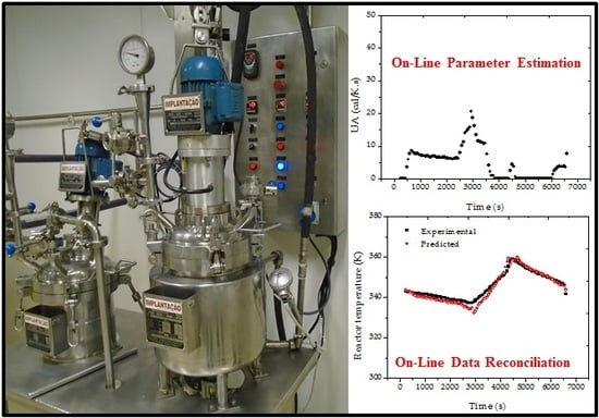
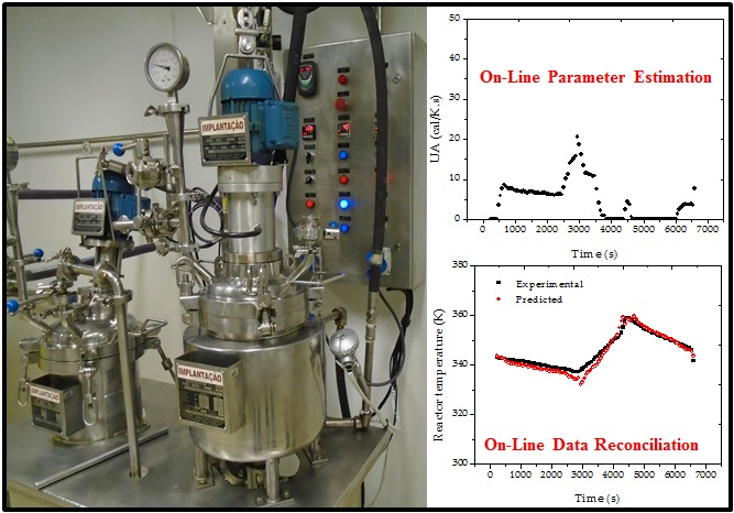
:A phenomenological model was developed to describe the dynamic evolution of the batch suspension polymerization of methyl methacrylate in terms of reactor temperature, pressure, concentrations and molecular properties of the final polymer. Then, the phenomenological model was used as a process constraint in dynamic data reconciliation procedures, which allowed for the successful monitoring of reaction variables in real-time and on-line. The obtained results indicate that heat transfer coefficients change significantly during the reaction time and from batch to batch, exerting a tremendous impact on the process operation. Obtained results also indicate that it can be difficult to attain thermodynamic equilibrium conditions in this system, because of the continuous condensation of evaporated monomer and the large mass transfer resistance offered by the viscous suspended droplets.
1. Introduction
Polymer materials are process products, as there are strong correlations between the final resin properties and the process operation conditions [1]. For this reason, and also considering that most polymer properties are difficult to measure at the plant site, mathematical models find widespread use in this field for the purposes of process control, monitoring, optimization of operation and product performance, scaling up, product design, and minimization of production costs, among other uses [2,3,4].
It is important to emphasize that most polymerization models present an inherent complexity, due to the nonlinear character of the correlations among the many process variables and the need to determine many kinetic and physico-chemical parameters, which are often unknown [1,5]. Besides, in order to describe and estimate adequately the end-use properties of interest, it may be necessary to develop relationships between the polymer quality variables (such as the melting flow index, the flexural modulus, the impact resistance, among others) and the final molecular properties of the resin (such as the molecular weight distribution, the chain composition distribution, the degree of branching, among others) [6,7]. The selection of the most adequate level of model sophistication for a particular application constitutes an important practical issue, as more detailed mathematics can provide more accurate model estimates, but can also lead to unfeasible applications, due to excessive computer demand.
One of the most important characteristics of polymerization kinetics and an important source of complexity is the fact that many polymerization reaction systems are limited by diffusion due to the high viscosities of concentrated polymer solutions, as the diffusion of growing polymer chains (and also of small molecules, if the polymer concentration is sufficiently high) can be significantly reduced, leading to the modification of the rate constants that govern the many reaction steps of the reaction mechanism [6]. In free-radical reactions, the reduced mobility of growing chains can lead to a reduction of the rates of chain termination (the well-known gel effect) and, consequently, to an acceleration of reaction rates and a shifting of molar mass distributions towards larger chain sizes, eventually causing reaction runaway. If the polymer concentration is sufficiently high, diffusion limitations can also affect the rates of propagation (the so called glass effect), limiting the maximum attainable monomer conversions and the initiator efficiency (the cage effect), affecting the course of the reaction. The high viscosities can also pose serious constraints on the rates of heat transfer, affecting the safety of the operation.
During the polymer production step, it is very important to keep the variables that define the polymer quality within well-defined ranges of acceptance and monitor the performances of important reactor operation constraints, such as the refrigeration capacity of the reactor. Therefore, model-based operation strategies of real polymerization processes may depend strongly on the reliable representation of the diffusion-limited reactions. For this reason, different approaches have been proposed to deal with diffusion-limited reaction phenomena, including the use of empirical correlations built with available experimental data and of more fundamental equations based on the free volume theory [8,9,10,11,12].
The lack of instrumentation to measure the vast majority of the important polymer end-use properties on-line has been largely recognized as one of the most important and challenging problems for the control and optimization of polymerization reactors [6]. Usually, on-line measurements, even when available, may offer poor reliability, long time delays, difficulties for appropriate sampling, among other problems. For this reason, new techniques have been developed for real-time and in-line monitoring of polymerization processes, many of them using optical fibers, including near-infrared spectroscopy (NIRS), midrange infrared spectroscopy (MIR), Raman spectroscopy, fluorescence spectroscopy and ultraviolet reflection spectroscopy [6].
In this context, the implementation of data reconciliation techniques in real reaction environments can be particularly important. In short, data reconciliation techniques combine the available process measurements and a suitable process model to allow for estimation of process states and process parameters [13,14]. This can allow for the monitoring of unmeasured variables (such as the end-use and molecular properties of the polymer material), also allowing for the enhancement of process reliability (as measured data are checked with the process model, which can include mass and energy balance equations). Consequently, data reconciliation can also open opportunities for implementation of fault detection schemes, reduction of process variability and development of soft-sensors. Particularly, soft-sensors can provide accurate inferences about important properties that are difficult to measure or additional redundant values for important operation values, providing means to monitor the performances of process instrumentation and making process operation safer.
The implementation of data reconciliation schemes in real polymerization processes has not been reported very frequently. Prata et al. [14] developed and implemented a robust procedure to solve the problem of dynamic data reconciliation, state estimation and parameter estimation in a continuous bulk propylene polymerization process. The authors were able to estimate unmeasured process states in real-time and at plant site based on a dynamic phenomenological process model. Souza et al. [15] developed and implemented a data reconciliation scheme for monitoring and control of the rate of polymerization and of final properties of carboxylated styrene-butadiene rubbers produced in batch reactors. The soft-sensor was used for the implementation of a predictive controller, enabling the optimization of the process operation in real-time. Lucia et al. [16] investigated the implementation of reconciliation schemes for optimization of sequences of batch emulsion polymerizations. The proposed approach was shown to provide major advantages in cases where only noisy measurements are available and uncertainties in the estimation are present. Rincón et al. [17] followed a similar line of investigation and presented a reconciliation scheme for monitoring of emulsion polymerization reactions performed in batch reactors, focused specifically on the estimation of monomer conversion and overall heat transfer coefficients.
It is important to emphasize that, to the best of our knowledge, data reconciliation schemes have never been used for the monitoring and control of suspension polymerization reactors. These reaction systems can offer many important challenges for implementation of this type of technology. First, suspension polymerizations are always performed in batch mode and are relatively fast. For instance, suspension polymerizations of methyl methacrylate are usually performed within a couple of hours, which means that computational algorithms must be efficient to provide reliable results after only a few minutes of operation, as there is not enough time for long periods of initial training and convergence. Second, polymer material tends to stick to the reactor internals during the reactor operation and accumulate from batch-to-batch, meaning that process parameters (such as the heat transfer coefficient) can change significantly during each batch and along the many successive batches, as reactor cleaning cannot be performed after the end of each individual reaction run. Third, the operation conditions (such as temperature and system viscosity) can change over the entire operation trajectory, reinforcing the importance of using reliable dynamic nonlinear models to describe the reaction course. Fourth, given the narrow operation window that assures the safety of the operation and the quality of the resin, it is very important to monitor the properties of the material accurately and to be able to control the operating conditions over the entire length of the batch.
Based on the previous discussion, a phenomenological model is developed to describe the dynamic evolution of the suspension polymerization of methyl methacrylate in terms of reactor temperature, pressure, concentrations and molecular properties of the final polymer. Numerical consistency tests of the mathematical model are evaluated in order to analyze the efficiency and the sensitivity of the model in respect to the most important process variables. The phenomenological model is then used as process constraint in dynamic data reconciliation procedures, which can allow for the successful monitoring of reaction variables in real time and on line. As shown in the following sections, the obtained results indicate the potential application of the proposed data reconciliation scheme as a soft-sensor for batch suspension methyl methacrylate polymerization processes, for monitoring and control purposes, allowing for improvement of the operating strategies of the plant.
2. Mathematical Modeling
The proposed mathematical model is used here to describe the evolution of the following output variables: reactor temperature, reactor pressure, monomer conversion, weight-average molar mass (Mw) and the polydispersity index (IP) of the polymer resin. The first two variables are related to the reactor operation and are usually available for monitoring purposes at plant site. Monomer conversion is related to the reactor productivity and exerts significant impact on post-reaction operation of the plant. Mw and IP can be used for off-line computation of end-use properties and are used at the plant site for product specification. The reaction mechanism of methyl methacrylate polymerization in suspension follows the usual free radical scheme, including the well-known kinetic steps of initiation, propagation, chain transfer to monomer and termination by disproportionation. Constitutive equations can be used to describe the gel effect and the glass effect. Based on this mechanism, mass and energy balance equations can be derived to describe the course of the reaction system, as showed in Appendix A. Model parameters are available in the open literature (Table 1).
The proposed mathematical model takes into account (i) the elementary and irreversible reaction steps; (ii) the negligible spatial gradients for all state variables inside the reactor; (iii) the additivity of volumes of individual species; (iv) the validity of the long chain approximation for kinetic rate constants; (v) the validity of the quasi-steady state assumption for radicals and statistical moments of living chains; (vi) the presence of air in the top empty space of the reactor (referred here as inert); (vii) ideal gas behavior; (viii) the negligible generation of heat by the mechanical agitator; (ix) the negligible dynamics of pipes and fittings. The resulting set of differential-algebraic equations was integrated with help of the numerical integrator DASSL (Differential-Algebraic System Solver), which is based on an implicit discretization method [18]. Numerical codes were implemented in Fortran in a desktop computer. The well-known method of moments was used to allow for the calculation of average molar masses and polydispersities. Similar models have been presented and used successfully by other authors to describe polymerizations of methyl methacrylate [19,20,21,22].
3. Simulations
3.1. Sensitivity Analysis of the Mathematical Model
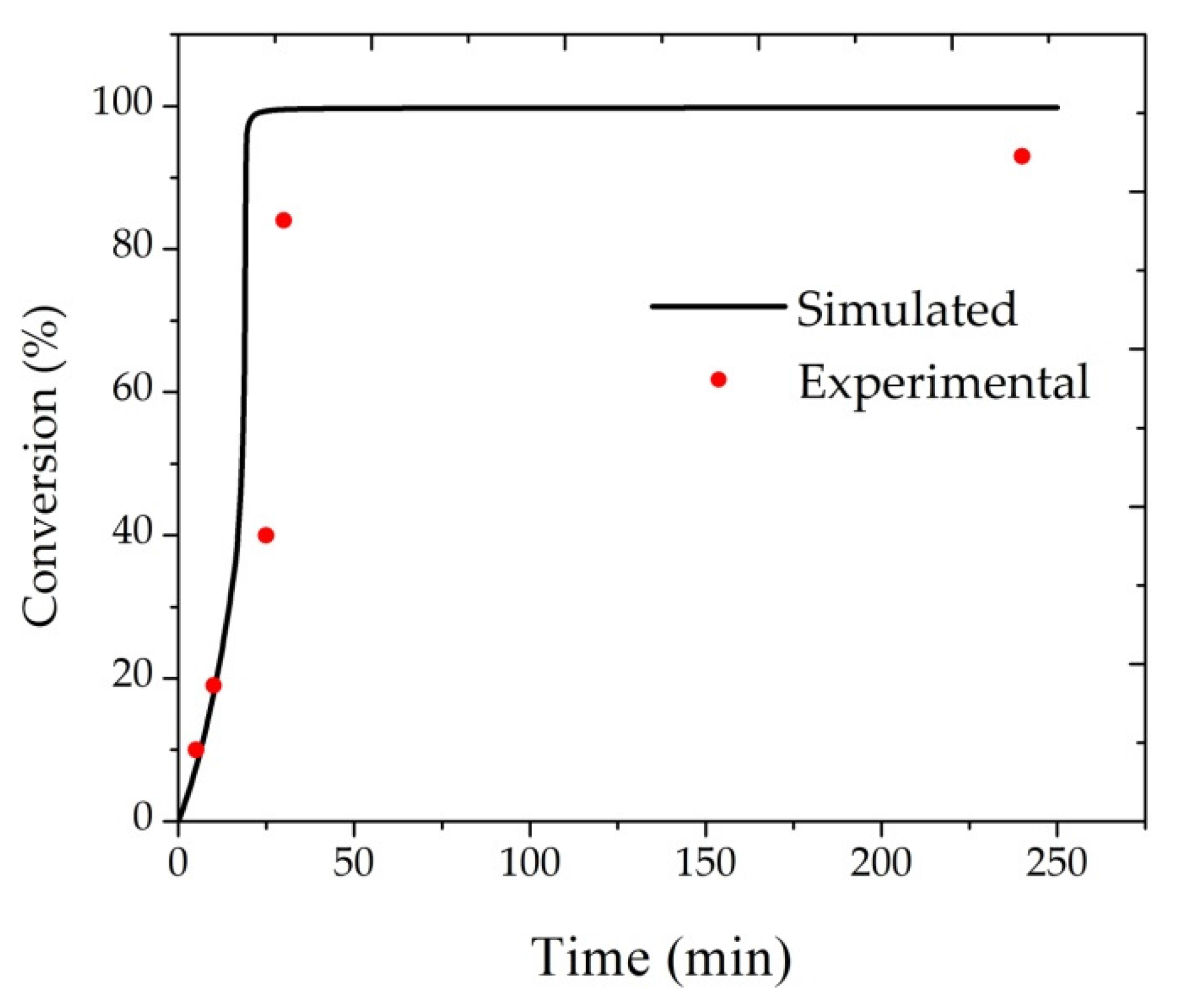
Before analyzing the sensitivity of the mathematical model in respect to important operation variables, it is necessary to confirm the validity of the simulations with actual experimental data as available in the literature [19,20,21,22]. For instance, Santos [23] studied the suspension polymerization of methyl methacrylate using a lab-scale reactor (with 1 L volume), benzoyl peroxide as initiator and poly(vinyl alcohol) (PVA) as the suspending agent. For reactions performed with 4 g of initiator, 2 g/L of PVA in the aqueous phase, 150 g of monomer and 450 g of water at 85 °C, the obtained experimental data were the ones presented in Figure 1. As one can observe in Figure 1, there is good agreement between reported and predicted monomer conversions, indicating good model performance. Besides this, Santos [23] reported a weight-average molecular weight of 4.1 × 10⁵ g/gmol for the final polymer resin, which can be easily tuned through the proper manipulation of the chain transfer constant to monomer or impurities, as the predicted weight-average molecular weight of the final polymer resin in absence of chain transfer was equal to 7.1 × 10⁵ g/gmol.
In order to verify the numerical consistency of the model simulations and simultaneously evaluate the sensitivity of the process responses to disturbances of the operation variables, some simulations were proposed, subject to the nominal conditions shown in Table 2, used to operate a real 10 L pilot plant reactor. Unless stated otherwise, the conditions described in Table 1 were kept the same in all simulations and used to perform the experiments in the pilot plant reactor.
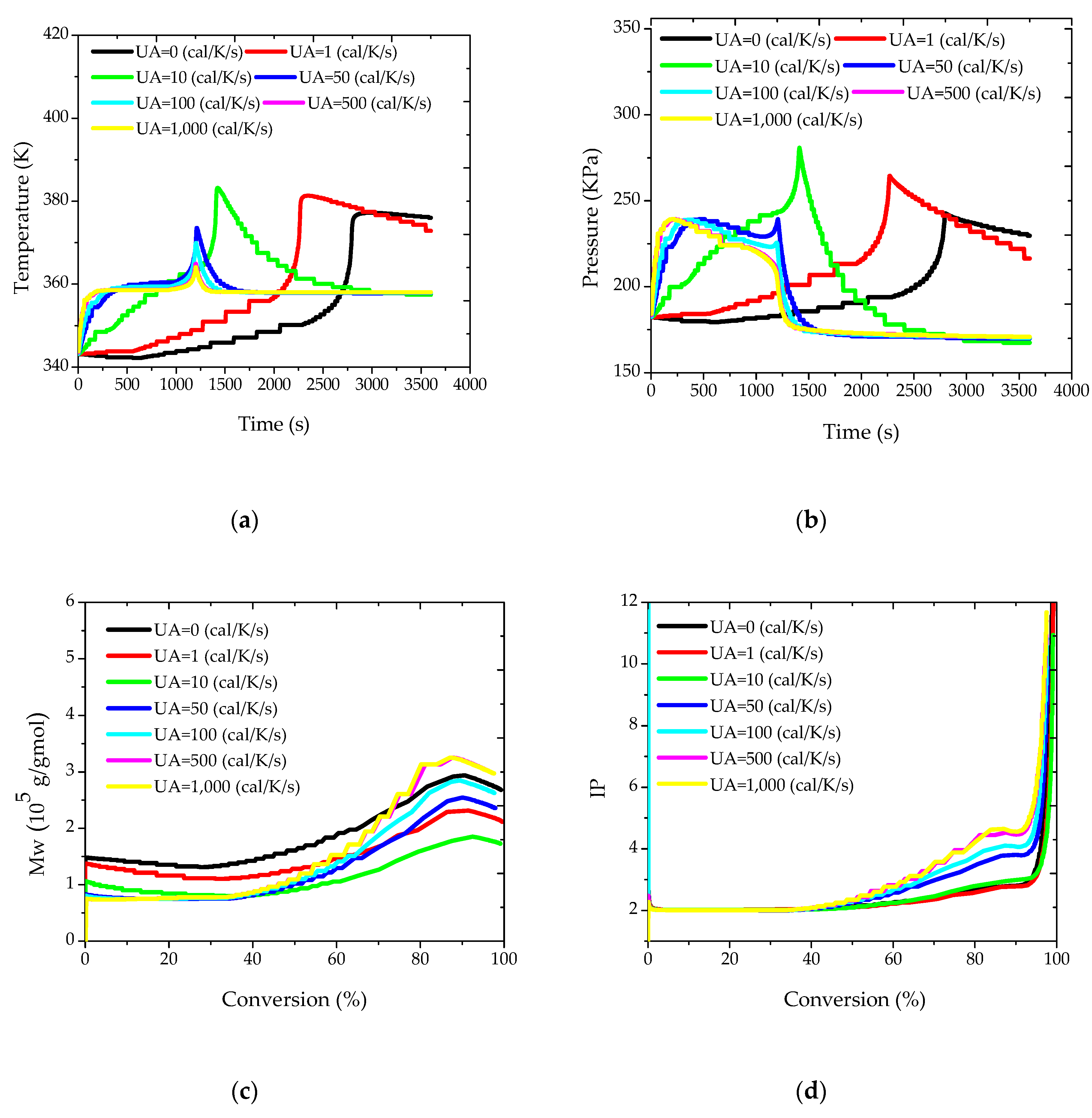
Initially, different values were considered for the overall heat transfer coefficient, allowing for the evaluation of the capacity of the jacket to remove the heat released by the reaction. As already stated, these simulations make sense because the heat transfer coefficients are expected to change within the batch and along the distinct batches. Simulation results are presented in Figure 2. It is interesting to observe that, in all cases, the jacket was not able to keep the reactor temperature constant and equal to the set-point value of 85 °C, despite the relatively low reactor volume, given the tremendous impact of the gel effect on the reactor operation. As a matter of fact, when the monomer conversion reaches approximately 50%, the reaction rate becomes so high that it is not possible to avoid the undesired heat kick of the reaction, which can lead to temperature increase of almost 30 °C when UA is equal to 50 cal/(K·s), as shown in Figure 2a. This certainly explains why many industrial facilities operate suspension methyl methacrylate polymerization reactors in adiabatic mode and give up the tight control of the reactor temperature trajectory (the rapid increase of the reactor temperature demands an extremely rapid change of the jacket temperature, which may not be feasible in real reactor setups). The adiabatic trajectory is shown in Figure 2a for sufficiently small values of UA, which leads to much longer reaction times (in industrial facilities, the reaction kick-off would be accelerated through heating until the desired initial reactor temperature and by keeping the jacket warm). Figure 2b shows that the reactor pressure follows the temperature trajectory, so that the safety of the reactor operation is closely related to the temperature control.
Regarding the molecular properties of the produced polymer, Figure 2c shows that higher values of the heat transfer coefficient cause the initial decrease of Mw values, given the higher reaction temperatures. However, the onset of the gel effect and the length and magnitude of the heat kick exert a dramatic effect on the final polymer properties, leading to more complex nonlinear responses. Similar words can be used to describe the trajectories of polydispersity indexes, which are initially close to 2 (as expected for free radical polymerizations controlled by disproportionation) but increase significantly during the heat kick phase. This is very interesting and indicates that it can be difficult to build simple correlations between the heat transfer coefficient and the final polymer properties. Apparently, this effect has never been described before, perhaps because most simulation and experimental studies assume that it is possible to keep the reaction temperature constant in these reaction processes.
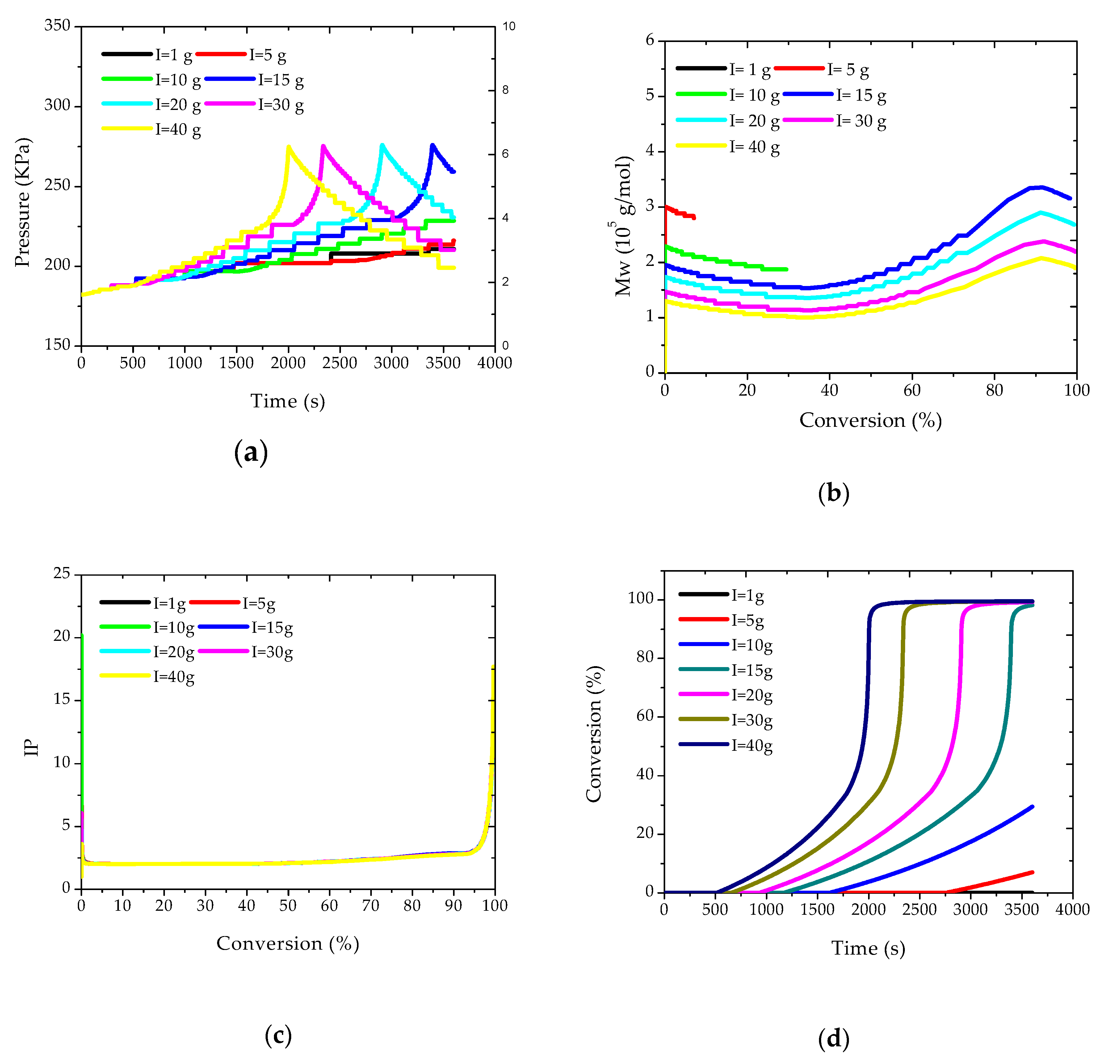
The effects caused by disturbances of the initial amounts of initiator on some of the state variables were also evaluated. These simulations make sense because the initiator can be used at the plant site for the control of some of the final polymer properties, defining some distinct polymer grades. Simulations are shown in Figure 3. Figure 3a shows that larger amounts of initiator cause the reactor pressure (and temperature) to increase in shorter periods of reaction, as expected, due to the higher rates of reaction, as also shown in Figure 3d.
However, it is very interesting to observe that the maximum pressure values were essentially constant in all cases, as these values are strongly correlated with the maximum adiabatic reaction temperature, which is reached closely during the heat kick period.
Figure 3b,c show that Mw values tend to decrease with the initial load of initiator, which might already be expected, and that polydispersity indexes are not very sensitive to this operation variable, being controlled by the onset of the gel effect and the heat kick conditions. Figure 3b also shows that Mw values tend to decrease in the beginning of the reaction, due to monomer consumption, then experience a consistent increase due to the gel effect, and finally tend to decrease again due to the onset of the glass effect.
3.2. Softsensor Formulation
After characterizing the appropriate behavior of the model responses, the use of the model as a soft-sensor is encouraged. In order to do this, the data reconciliation problem was formulated as presented below. It is assumed that a certain objective function must be minimized, while subjected to model and operation constraints, through manipulation of certain sets of reconciled values (), model parameters () and unmeasured variables () [5].
Objective function:
- Model and operation constraints:
- Search space:
In Equation (1), is the vector of measured variables. The index denotes the lower search limit, while the index s represents the upper search limit. In the traditional approach, the objective function has the form of weighted least squares:
where represents the number of measured sampling points and represents the variance of the ith measurement. In a more general formulation, the objective function has the form of the maximum likelihood function:
where is the covariance matrix of measurements. When measurements are independent, the covariance matrix of measurements becomes diagonal and Equation (8) becomes equal to Equation (7). In this form, the data reconciliation procedure is designed to estimate the “true” unknown measurements () with the estimate of the process variability () and the process constraints provided by the mathematical model [24].
The numerical procedure used to solve the proposed data reconciliation problem was based on stochastic particle swarm optimization, using the objective function given by Equation (8) [25]. The particle swarm technique is a stochastic procedure that performs the optimization through the combination of stochastic sampling in the search space (particles) and the exchange of information between particles during the successive iterations of the numerical procedure. The technique consists essentially in generating at random a set of initial estimates for the decision variables (particles) in the search space and updating the estimates based on the best objective function estimates obtained by the group of particles (swarm). The update is based on the moving speed of each particle (v), initially set at random and then corrected to allow movement towards the best sampled estimates [25]. In a simple way, the algorithm proposes that:
where is the estimate at iteration k, is the speed at iteration , is the best estimate obtained by the particle, is the best estimate obtained by the swarm (with Npt particles), and , , and are tuning parameters. , and are random numbers distributed uniformly in the interval [0,1].
Two stopping criteria are generally used in particle swarm algorithms. The first one imposes a maximum number of iterations (Niter) on the numerical procedure, while the second one defines a convergence criterion for the objective function between successive iterations (TOL) [25].The tuning parameters used in the simulations performed in the present manuscript are described in Table 3.
3.3. Process
Reactions were performed in a 10 L stainless steel pilot plant reactor, using the nominal operation conditions presented in Table 2. The effect of the agitation speed on the pilot plant performance was investigated as defined in Table 4. Reactor temperature, jacket temperature and reactor pressure were measured by the data acquisition software and stored as minute averages. These values were used as measured inputs for the proposed data reconciliation problem.
Gel permeation chromatography (GPC, also known as chromatography by size exclusion) was employed to determine the average molar masses and molar mass distributions of polymer samples. To conduct the experimental analyses, polymer solutions were prepared in tetrahydrofuran (TFH) with concentration of 1 mg/mL. The solutions were filtrated with a teflon membrane with pore size of 0.45 μm. Then, approximately 200 μL of the filtrate were injected into the GPC equipment (Viscotek GPC Max VE 2001, Massachusetts, MA, USA), calibrated with poly(styrene) standards of molar masses between 5 × 10³ and 1 × 10⁶ g/gmmol, and equipped with three Shodex columns and a refractometer detector (Viscotek VE 3580, Massachusetts, MA, USA). The analyses were conducted at 40 °C.
The overall heat transfer coefficient (UA), the initial reactor temperature and the initial jacket temperature were estimated model parameters. Measurements of the initial temperatures were subject to uncertainties in the beginning of the reaction because of the reactor feed operation and procedures taken to seal the reactor top. The search regions used for estimation purposes are shown in Table 5.
The data reconciliation problem was solved with help of the traditional moving window strategy [5,24]. According to this dynamic strategy, when a new sampling point is available, the oldest sampling point is discarded, keeping the window size constant. This strategy is intended to capture the most recent behavior of the process at each iteration and to reduce the complexity in terms computational cost, avoiding the use of all available data. The moving window has a total dimension of H × NV, where H is the number of samples in the moving window and NV is the number of measured variables used for estimation purposes. In the present work, unless stated otherwise, H was always equal to 5. It is also important to emphasize that the computational time required to perform the calculations for each moving window always shorter than 2 s, thus much shorter than the sampling time of 1 min, therefore characterizing the potential for applications in real time.
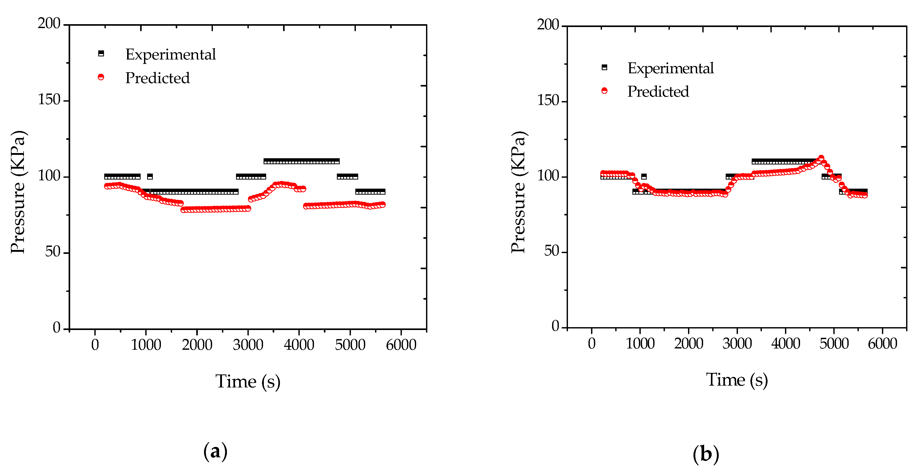
3.4. Adjustment of the Reactor Pressure
According to the traditional Flory–Huggins approach (Equations (A26)–(A28) of Appendix A), predicted reactor pressures experience smaller variations than the respective experimental measurements, as shown in Figure 4a. Although differences may be regarded as small, the fact is that these differences lead to significant variations of other process variables during the data reconciliation procedure, as shown in Figure 5. In short, as experimental pressures were higher than predicted, the estimator tended to compensate this effect by increasing the reactor temperature. Therefore, it was necessary to propose some adjustments to solve this problem. A corrective action assumed that fresh monomer droplets were always present inside the reactor. This hypothesis is consistent with the idea that the vaporized monomer condenses and forms new droplets of fresh monomer, so that the vapor pressure of the droplets remains essentially equal to the vapor pressure of the pure monomer throughout the course of the reaction. This hypothesis is also consistent with the idea that there are strong limitations to mass transfer of fresh condensed monomer to the interior of the polymer particles. In this case, Equation (A26) must be replaced by Equation (11), in the form:
When Equation (11) was used for data reconciliation purposes, the results obtained were much better and are shown in Figure 4b. Moreover, similar results were obtained for reaction R2. Thus, it can be said that Equation (11) was much better suited for the proposed analysis than the standard Flory–Huggins equation. This apparently suggests that equilibrium conditions may indeed be inadequate to describe the phase behavior in real polymerization reactors, possibly due to the existence of large mass transfer resistances and droplets of fresh condensed monomer, as previously discussed. Despite the importance of this particular issue, this point has been completely overlooked in the past, and perhaps should deserve more detailed attention in the near future, as similar problems are expected to occur in larger plants, especially when process condensers are used for removal of the heat of reaction.
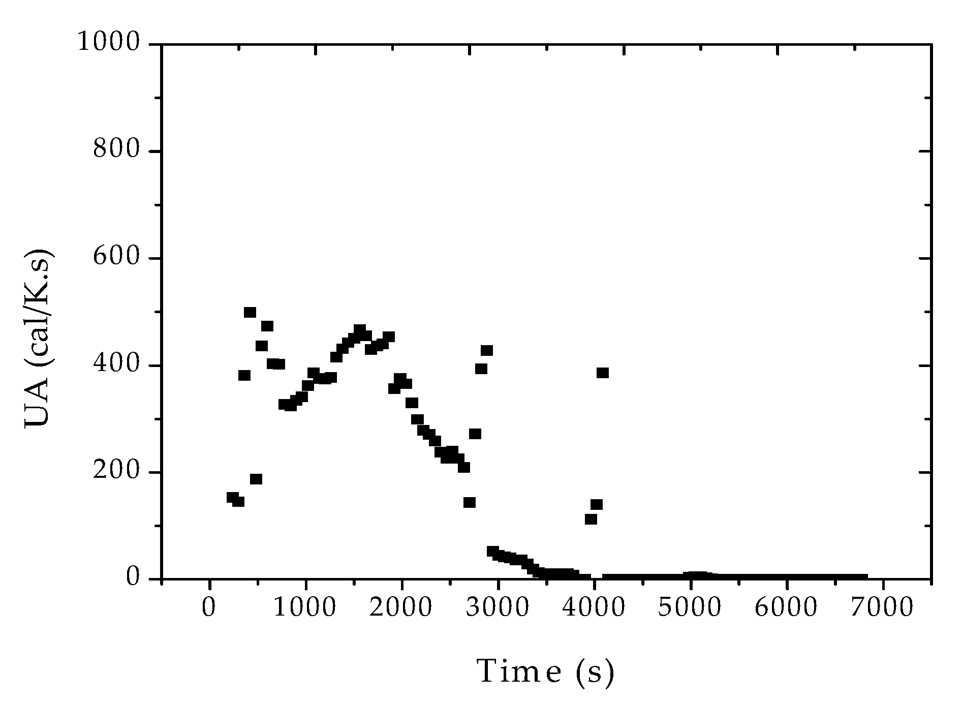
3.5. Process Monitoring
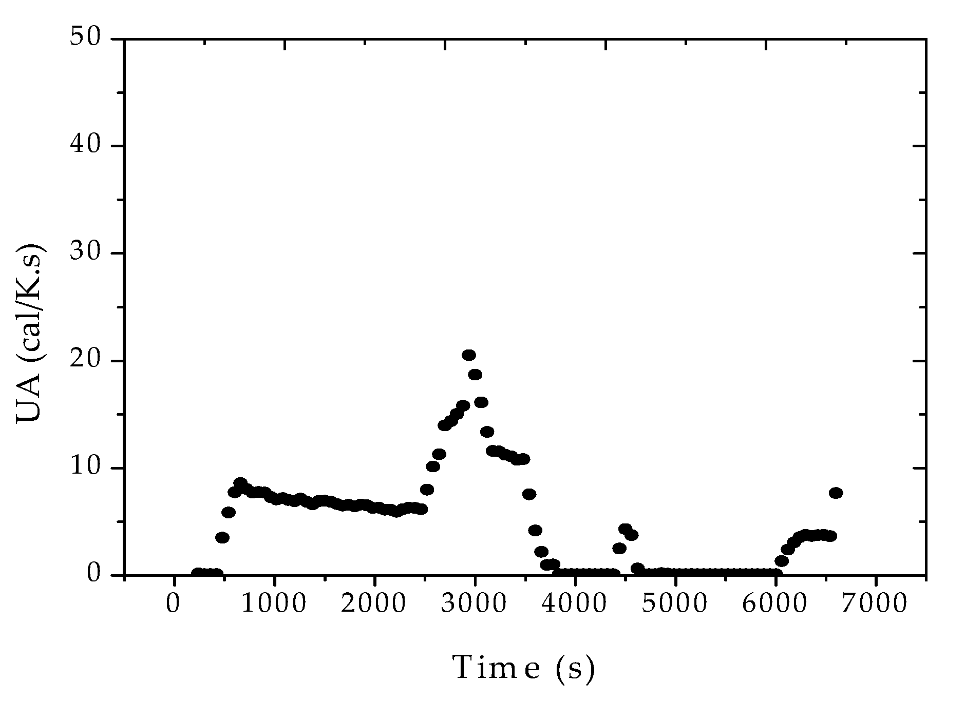
After the adjustment of the reactor pressure profiles, the proposed strategy was shown to be effective for the monitoring of the main process variables and of the final properties of the polymer resin, as shown in Figure 6. According to Figure 7, the heat transfer coefficient presented a clear decreasing trend during the batch. The sudden increase of UA after about 40 min of reaction was related to the increase of the jacket temperature, required to keep the reaction temperature closer to the desired set-point value. This clearly suggests the poorer heat transfer conditions of a more viscous reaction medium and the possible occurrence of fouling at the internal reactor walls. As a matter of fact, the accumulation of thin polymer films on the internal reactor walls could be detected visually at the end of the reaction trials, reinforcing the proposed assumption.
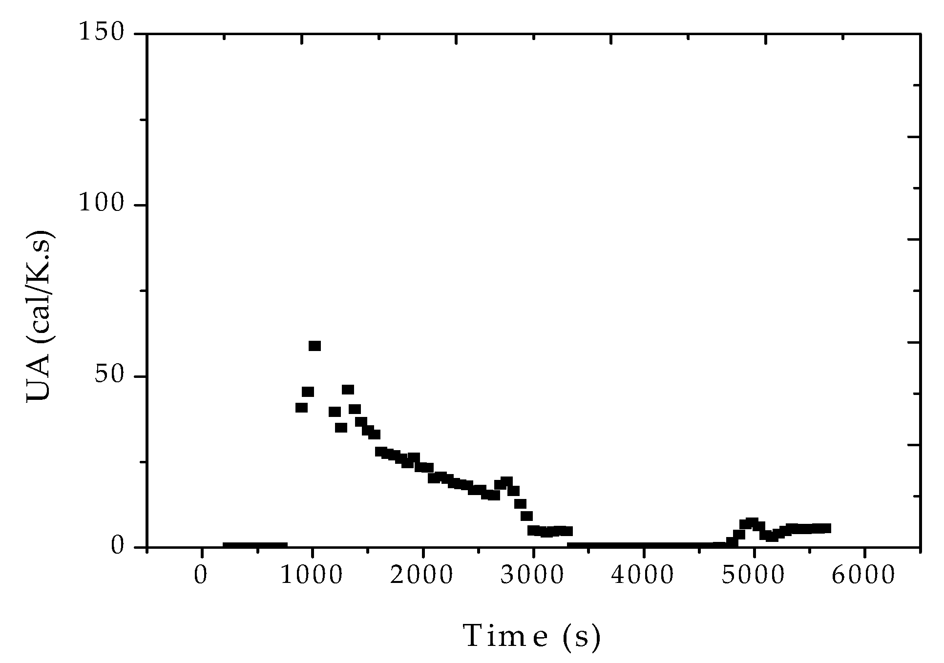
Figure 8 and Figure 9 show that similar decreasing dynamic heat transfer coefficient profiles were observed in the other two reaction experiments. However, it is very important to observe the huge sensitivity of the heat transfer coefficient in respect to the stirring rate, increasing with the increase of the stirring, as expected. This clearly indicates that heat transfer coefficients cannot be regarded as constant at the plant site, especially when the stirring rate is used as a manipulated variable for production of distinct polymer grades.
It was surprising to observe the huge variations experienced by the heat transfer coefficient in such a small reaction system (10 L) for such a short period of time (90 min). Based on these results, one can possibly expect even higher variations in large reaction vessels, given the difficulties in cleaning the reactor internals after every reaction run. The reduction of UA during the batch causes the increase of the reactor temperature, and consequently of reaction rates and conversion, demanding additional efforts from the controlling devices.
In order to evaluate the importance of UA variations during the batches, a different reconciliation strategy was proposed. According to the expansive window approach, when a new sampling point is available, the oldest sampling point is not discarded, increasing the window size. This strategy is intended to capture the complete behavior of the process through the use of all available data, assuming the existence of a single UA value to represent the whole experimental trajectory. By using the expansive window approach, however, the data reconciliation was not effective, because the reconciled values deviated very significantly from the experimental values. This result showed that variation of the heat transfer coefficient was indeed very important to allow for the proper fitting of the available data, and confirmed indirectly the occurrence of fast UA variations during the reactor operation.
4. Conclusions
It was shown that the simultaneous monitoring of different process variables (reactor temperature, reactor pressure, jacket temperature, heat transfer coefficient, monomer conversion, weight average molecular weight of the resin and polydispersity index of the resin) can be performed successfully in batch suspension polymerizations of methyl methacrylate at different operating conditions, with help of a phenomenological process model and of dynamic data reconciliation procedures. The data reconciliation procedure relied on three process inputs usually available at the plant site (reactor temperature, reactor pressure and jacket temperature) and could be solved in a desktop computer in less than 2 s with help of the stochastic particle swarm optimization procedure, allowing for implementation in real-time and on-line. Because of the strong nonlinear behavior of the analyzed process, sampling windows of 5 min and sampling intervals of 1 min were used for the iterative implementation of the computer code and fast adaptation to the evolving system trajectories.
Based on the obtained results, some points should be emphasized. Firstly, variations of the heat transfer coefficients can exert a tremendous effect on the process operation and final polymer properties, as they define the length and magnitude of the unavoidable heat kicks. Besides this, the increase of the system viscosity and accumulation of polymer film at the reactor walls lead to continuous decrease of heat transfer coefficients during the batch. Secondly, the continuous evaporation and condensation of monomer and the high mass transfer resistance offered by the viscous suspended droplets probably favor the formation of fresh monomer droplets, which can keep the reactor pressure higher than expected by thermodynamic equilibrium hypotheses. This assumption was validated indirectly through reconciliation of the available experimental data, using different thermodynamic equilibrium approaches.
Acknowledgments
The authors thank CAPES (Coordenação de Aperfeiçoamento de Pessoal de Nível Superior) and CNPq (Conselho Nacional de Desenvolvimento Científico e Tecnológico) for providing scholarships and supporting this work.
Conflicts of Interest
The authors declare no conflict of interest.
Symbols, Acronyms and Abbreviations
| Ai, Bi, Ci | Antoine constants |
| CpA | Heat capacity of water [cal/g·K] |
| CpC | Heat capacity of the cooling fluid [cal/g·K] |
| Cpi | Heat capacity of reactant i in the reacting medium [cal/g·K] |
| Cpm | Heat capacity of monomer [cal/g·K] |
| CpP | Heat capacity of polymer [cal/g·K] |
| Di | Dead polymer chains of length i [mol] |
| Fc | Volumetric flowrate of cooling fluid [g/s] |
| f | Initiator efficiency |
| gp | Glass effect contribution |
| gt | Gel effect contribution |
| −ΔH | Heat of reaction [kJ/mol] |
| I(0) | Initial initiator mass [g] |
| I | Initiator [mol] |
| Inib | Inhibitor [mol] |
| IP | Polydispersity |
| ki | Initiation rate constant [cm3/mol·s] |
| kd | Initiator decomposition rate constant [s−1] |
| kp | Propagation rate constant [cm3/mol·s] |
| ktd | Termination by disproportionation rate constant [cm3/mol·s] |
| ktm | Transfer to monomer rate constant [cm3/mol·s] |
| M(0) | Initial monomer mass [g] |
| M | Monomer [mol] |
| MMA | Molecular weight of water [g/gmol] |
| MA(0) | Initial water mass [g] |
| MMm | Molecular weight of monomer [g/gmol] |
| MMI | Molecular weight of initiator [g/gmol] |
| MMinert | Molecular weight of inert [g/gmol] |
| Mn | Number-average molecular weight [g/gmol] |
| MPVA(0) | Initial inhibitor mass [g] |
| Mw | Weight-average molecular weight [g/gmol] |
| ninert0 | Inert at the beginning of reaction [mol] |
| ninert | Inert at the end of reaction [mol] |
| PAsat | Water saturation pressure [kPa] |
| Pmmasat | Monomer saturation pressure [kPa] |
| P(0) | Atmospheric pressure [kPa] |
| Pi | Living polymer chains of length i [mol] |
| Pinert | Inert partial pressure [kPa] |
| Pisat | Saturation pressure of component i [kPa] |
| Ppi | Partial pressure of reactant i in the reacting medium [kPa] |
| QP | Rate of energy exchanged with the environment [cal/s] |
| QR | Rate of energy released by the polymerization reaction [cal/s] |
| QT | Rate of energy exchanged with jacket [cal/s] |
| R | Universal gas constant [J/mol·K] |
| R⦁ | Radicals [mol] |
| Rp | Propagation rate [mol/s] |
| T | Reactor temperature [K] |
| TA | Ambient temperature [K] |
| TC | Jacket temperature [K] |
| TeC | Input cooling fluid temperature [K] |
| Tgm | Glass transition temperature of monomer [K] |
| Tgp | Glass transition temperature of polymer [K] |
| t | Time [s] |
| UA | Heat transfer coefficient with reactor [cal/K·s] |
| UAA | Heat transfer coefficient with ambient [cal/K·s] |
| VA | Volume of water [L] |
| VL | Total volume of liquid phase [L] |
| VR | Total reactor volume [L] |
| VC | Jacket volume [L] |
| Vf | Total free volume of organic phase [mL] |
| Vfm | Contribution of monomer to free volume [mL] |
| Vfp | Contribution of polymer to free volume [mL] |
| Vfpc | Critical free volume for propagation [mL] |
| Vftc | Critical free volume for termination [mL] |
| Vm | Total volume of monomer [mL] |
| Vo | Total volume of organic phase [mL] |
| Vp | Total volume of polymer [mL] |
| X | Monomer conversion [%] |
| αm | Thermal expansion coefficient for monomer |
| αp | Thermal expansion coefficient for polymer |
| χ | Flory–Huggins interaction parameter |
| λK | kth moment of the chain-length distributions of living polymer chains |
| μK | kth moment of the chain-length distributions of dead polymer chains |
| φiv | Volumetric fraction of component i |
| φpv | Volumetric fraction of polymer |
| ρA | Water density [g/cm3] |
| ρp | Polymer density [g/cm3] |
| ρc | Cooling fluid density [g/cm3] |
| ρi | Density of reactant i [g/cm3] |
| ρm | Density of monomer [g/cm3] |
Appendix A
Mathematical Model
Initiator (benzoyl peroxide) molar balance:
Radical fragment molar balance:
Moments of the size distribution of living chains:
Moments of the size distribution of dead chains:
Monomer molar balance:
Inhibitor molar balance:
0th moment of the size distribution of living chains:
1st moment of the size distribution of living chains:
2nd moment of the size distribution of living chains:
0th moment of the size distribution of dead chains:
1st moment of the size distribution of dead chains:
2nd moment of the size distribution of dead chains:
Volume of the organic phase:
Number average molecular weight of the polymer:
Weight average molecular weight of the polymer:
Polydispersity:
Monomer conversion:
Gel effect and glass effect equations (based on the free volume theory):
Reactor pressure:
Inert gas molar balance:
Reactor energy balance:
Jacket energy balance:
References
- Latado, A.; Embiruçu, M.; Neto, A.G.M.; Pinto, J.C. Modeling of enduse properties of poly (propylene/ethylene) resins. Polym. Test. 2001, 20, 419–439. [Google Scholar] [CrossRef]
- Leiza, J.R. Sensors, Process Control and Modelling in Polymer Production. Macromol. React. Eng. 2009, 3, 324–325. [Google Scholar] [CrossRef]
- Mueller, P.A.; Richards, J.R.; Congalidis, J.P. Polymerization Reactor Modeling in Industry. Macromol. React. Eng. 2007, 5, 261–277. [Google Scholar] [CrossRef]
- Stoessel, F.; Ubrich, O. Safety assessment and optimization of semi-batch reactions by calorimetry. J. Therm. Anal. Calorim. 2001, 64, 61–74. [Google Scholar] [CrossRef]
- Prata, D.M. Robust Data Reconciliation for Real-Time Monitoring. Ph.D. Thesis, COPPE/UFRJ, Rio de Janeiro, Brazil, 2009. [Google Scholar]
- Giudici, R. Polymerization reaction engineering: A personal overview of the state-of-art. Lat. Am. Appl. Res. 2000, 30, 351–356. [Google Scholar]
- Quelhas, A.D.; Jesus, N.J.C.; Pinto, J.C. Common vulnerabilities of RTO implementations in real chemical processes. Can. J. Chem. Eng. 2013, 91, 652–668. [Google Scholar] [CrossRef]
- Friis, N.; Hamielec, A.E. Gel effect in emulsion polymerization of vinyl monomers. ACS Symp. Ser. 1976, 24, 82–91. [Google Scholar]
- Marten, F.L.; Hamielec, A.E. High conversion diffusion-controlled polymerization. ACS Symp. Ser. 1979, 104, 43–70. [Google Scholar]
- Chiu, W.Y.; Carrat, G.M.; Soong, D.S. A computer model for the gel effectin free-radical polymerization. Macromolecule 1983, 16, 348–357. [Google Scholar] [CrossRef]
- Ray, A.B.; Saraf, D.N.; Grupta, S.K. Free radical polymerizations associated with Trommsdorff effect under semibatch reactor conditions: I. Modeling. Polym. Eng. Sci. 1995, 35, 1290–1299. [Google Scholar] [CrossRef]
- Pinto, J.C.; Ray, W.H. The Dynamic Behavior of Continuous Solution Polymerization Reactors—VII. Experimental study of a Copolymerization Reactor. Chem. Eng. Sci. 1995, 50, 715–736. [Google Scholar] [CrossRef]
- Bai, S.; Mclean, D.D.; Thinbault, J. Impact of Model Structure on the Performance of Dynamic Data Reconciliation. Comput. Chem. Eng. 2007, 31, 127–135. [Google Scholar] [CrossRef]
- Prata, D.M.; Schwaab, M.; Lima, E.L.; Pinto, J.C. Nonlinear Dynamic Data Reconciliation in Real Time in Actual Processes. Comput. Aided Chem. Eng. 2009, 27, 47–54. [Google Scholar]
- Souza, P.N.; Soares, M.; Amaral, M.M.; Lima, E.L.; Pinto, J.C. Data Reconciliation and Control in Styrene-Butadiene Emulsion Polymerizations. Macromol. Symp. 2011, 302, 80–89. [Google Scholar] [CrossRef]
- Lucia, S.; Finkler, T.; Engell, S. Multi-stage Nonlinear Model Predictive Control Applied to a Semi-Batch Polymerization Reactor under Uncertainty Prediction Horizon. J. Process Control 2013, 23, 1306–1319. [Google Scholar] [CrossRef]
- Rincón, F.D.; Esposito, M.; Araújo, P.H.H.; Lima, F.V.; LE Roux, G.A.C. Robust Calorimetric Estimation of Semi-Continuous and Batch Emulsion Polymerization Systems with Covariance Estimation. Macromol. React. Eng. 2014, 8, 456–466. [Google Scholar] [CrossRef]
- Petzold, L.R. DASSL Code; version 1989; Computing and Mathematics Research Division, Lawrence Livermore National Laboratory: Livermore, CA, USA, 1989.
- Melo, C.K.; Soares, M.; Castor, C.A.; Melo, P.A.; Pinto, J.C. In Situ Incorporation of Recycled Polystirene in Styrene Suspension Polymerizations. Macromol. React. Eng. 2014, 8, 46–60. [Google Scholar] [CrossRef]
- Brandrup, J.; Immergut, E.H.; Grulke, E.A. Physical Constants of Some Important Polymers. In Polymer Handbook, 4th ed.; Brandrup, J., Edmund, H., Immergut, E., Grulke, A., Abe, A., Bloch, D.R., Eds.; Wiley: New York, NY, USA, 1999; pp. 1–2336. [Google Scholar]
- Perry, R.H.; Geen, D.W. (Eds.) Physical and Chemical Data. In Perry’s Chemical Engineers’ Handbook, 7th ed.; McGraw-Hill: New York, NY, USA, 1997; pp. 1–2640. [Google Scholar]
- Smith, J.M.; Van Ness, H.C.; Abbott, M.M. Thermodynamic Properties of Fluids. In Introduction to Chemical Engineering Thermodynamics, 7th ed.; Glandt, E.D., Klein, M.T., Edgar, T.F., Eds.; McGraw-Hill: New York, NY, USA, 2007; Volume 1, pp. 1–807. [Google Scholar]
- Santos, J.R. Monitoring and Control of Particle Sizes in MMA Suspension Polymerizations Using NIRS. Ph.D. Thesis, COPPE/UFRJ, Rio de Janeiro, Brazil, 2012. [Google Scholar]
- Liebman, M.J.; Edgar, T.F.; Lasdon, L.S. E-cient Data Reconciliation and Estimation for Dynamic Processes Using Nonlinear Programming Techniques. Comput. Chem. Eng. 1992, 16, 963–986. [Google Scholar] [CrossRef]
- Schwaab, M.; Biscaia, E.C., Jr.; Monteiro, J.L.; Pinto, J.C. Nonlinear Parameter Estimation through Particle Swarm Optimization. Chem. Eng. Sci. 2008, 63, 1542–1552. [Google Scholar] [CrossRef]
Figure 1.
Monomer conversion, as provided by the model and reported by Santos [23].
Figure 1.
Monomer conversion, as provided by the model and reported by Santos [23].

Figure 2.
(a) Temperature; (b) pressure; (c) weight-average molar mass (Mw); and (d) polydispersity index (IP) profiles for different values of the overall heat transfer coefficient.
Figure 2.
(a) Temperature; (b) pressure; (c) weight-average molar mass (Mw); and (d) polydispersity index (IP) profiles for different values of the overall heat transfer coefficient.

Figure 3.
(a) Pressure; (b) Mw; (c) IP; and (d) conversion profiles for different initial loads of initiator.
Figure 3.
(a) Pressure; (b) Mw; (c) IP; and (d) conversion profiles for different initial loads of initiator.

Figure 4.
(a) Reconciled pressure profiles for reaction R1, considering (a) the traditional equilibrium approach and (b) the existence of fresh monomer droplets.
Figure 4.
(a) Reconciled pressure profiles for reaction R1, considering (a) the traditional equilibrium approach and (b) the existence of fresh monomer droplets.

Figure 5.
Reconciled reactor temperature profiles for reaction R2 considering the traditional equilibrium approach.
Figure 5.
Reconciled reactor temperature profiles for reaction R2 considering the traditional equilibrium approach.
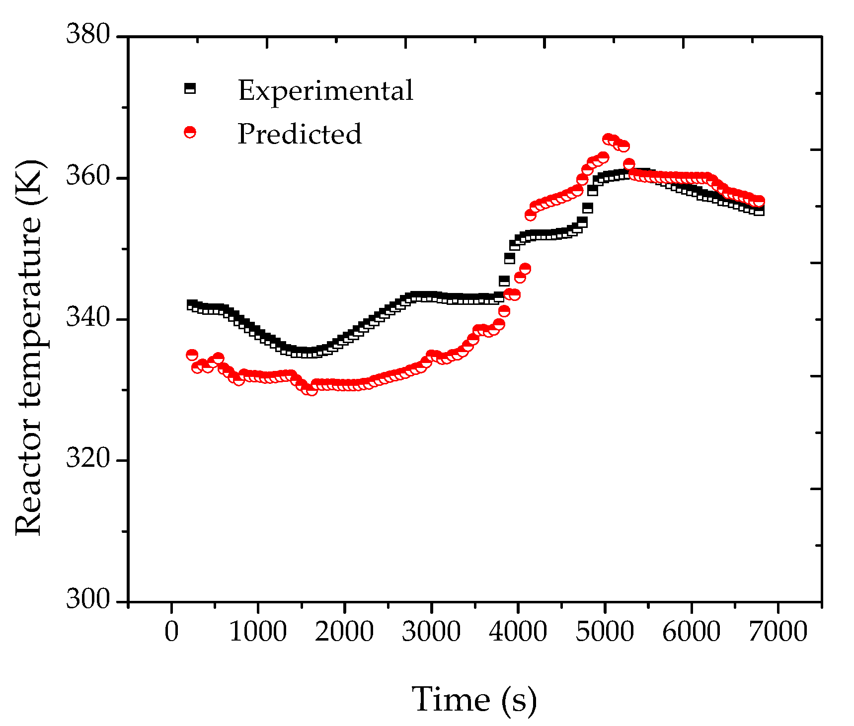
Figure 6.
Reconciled (a) reactor temperature; (b) reactor pressure; (c) jacket temperature; (d) IP; (e) Mw; (f) conversion profiles for reaction R3, considering the formation of fresh monomer droplets.
Figure 6.
Reconciled (a) reactor temperature; (b) reactor pressure; (c) jacket temperature; (d) IP; (e) Mw; (f) conversion profiles for reaction R3, considering the formation of fresh monomer droplets.
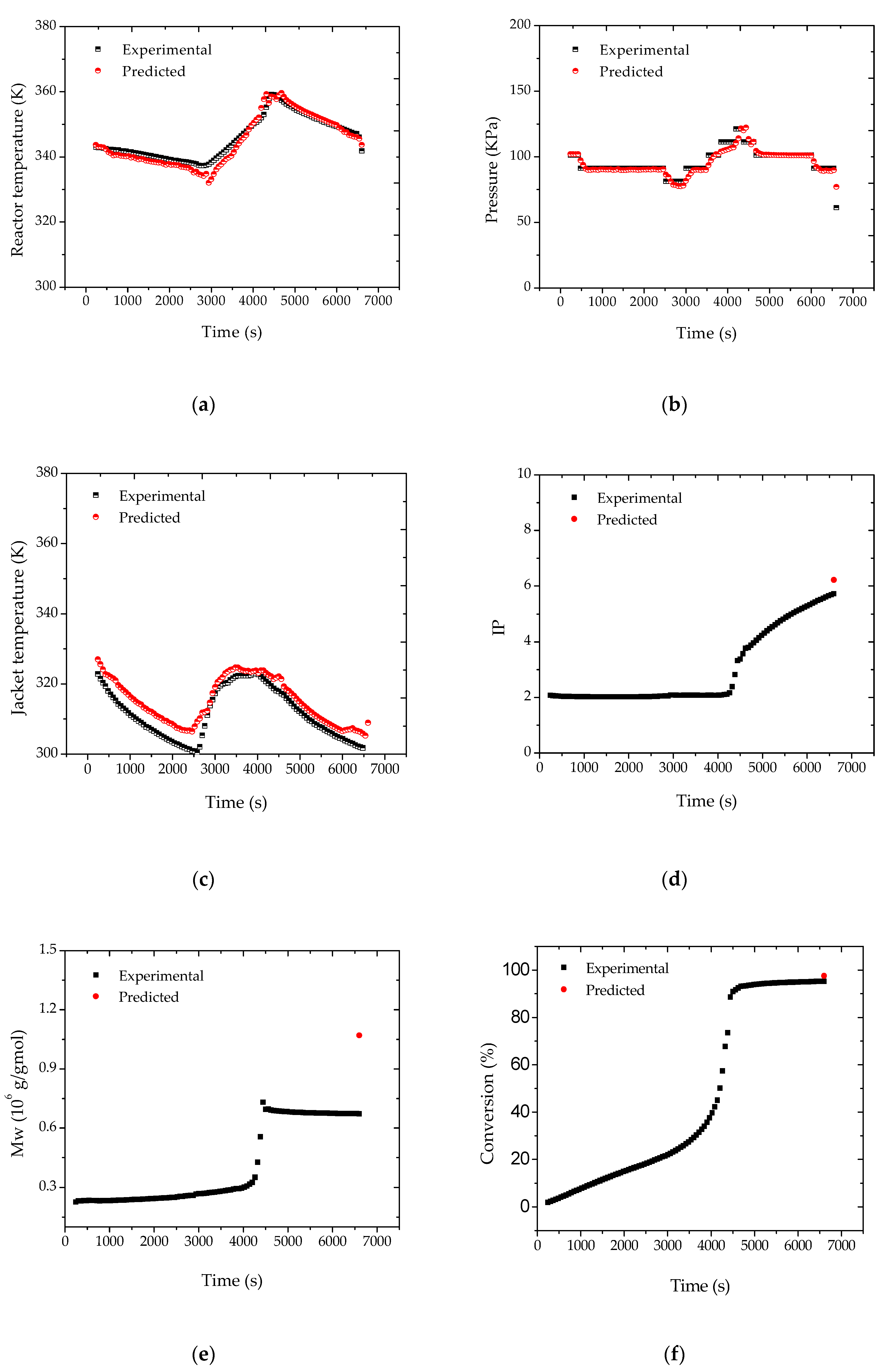
Figure 7.
Reconciled UA profiles for reaction R3, considering the formation of fresh monomer droplets.
Figure 7.
Reconciled UA profiles for reaction R3, considering the formation of fresh monomer droplets.

Figure 8.
Reconciled UA profiles for reaction R1, considering the formation of fresh monomer droplets.
Figure 8.
Reconciled UA profiles for reaction R1, considering the formation of fresh monomer droplets.

Figure 9.
Reconciled UA profiles for reaction R2, considering the formation of fresh monomer droplets.
Figure 9.
Reconciled UA profiles for reaction R2, considering the formation of fresh monomer droplets.

Table 1.
Parameters and variables of the mathematical model. 1
| Parameters | References |
|---|---|
| kd = 1.7 × 10¹⁴∙exp(−30000/RT) s−1 | [19] |
| kp = 7 × 10⁹gp∙exp(−6300/RT) cm3/mol·s | [12] |
| ktd = 1.76 × 10¹² gt∙exp(−2300/RT) cm3/mol·s | [12] |
| ktm = kp∙exp(−2.6 − 2888/T) cm3/mol·s | [20] |
| f = 0.6 | [12] |
| [12] | |
| [12] | |
| [21] | |
| MMm = 100.12 g/gmol | [21] |
| MMinert = 28.0 g/gmol | [22] |
| MMA = 18.0 g/gmol | [21] |
| MMI = 242.3 g/gmol | [21] |
| Cpm = 0.49 cal/g∙KCpA = 1.0 cal/g∙K | [12,21] |
| [12] | |
| [12] | |
| [22] | |
| ∆H = 57.7 kJ/mol | [12] |
| αm = 0.001 | [12] |
| Tgm = 167 K | [12] |
| αp = 0.00048 | [12] |
| Tgp = 387 K | [12] |
| χ = 0.5 | [12] |
| VC = 10 L | Location data |
| VL = 15 L | Location data |
| Fc (g/s) | Location data |
| UAA (cal/K·s) | Location data |
1-Symbols and acronyms are presented at the end of the manuscript.
Table 2.
Nominal operating conditions used to perform numerical simulations.
| Operational Condition | Value |
|---|---|
| T(0) (K) | 343.15 |
| Tc(0) (K) | 358.15 |
| Tec (K) | 373.15 |
| Fc (g/s) | 200.0 |
| UA (cal/K·s) | 2 |
| UAA (cal/K·s) | 1.75 × 10⁻¹ |
| M(0) (g) | 1500 |
| I(0) (g) | 15 |
| MA(0) (g) | 4500 |
| MPVA(0) (g) | 45 |
| P(0) (atm) | 1 |
Table 3.
Particle swarm tuning parameters used to perform simulations.
| Npt | Niter | C1 | C2 | w | TOL |
|---|---|---|---|---|---|
| 50 | 200 | 1 | 1 | 0.7 | 10−3 |
Table 4.
Agitation speeds in the different reaction runs.
| Reaction | Stirring Rate in the First 10 Min (rpm) | Stirring Rateafter 10 Min (rpm) |
|---|---|---|
| R1 | 800 | 600 |
| R2 | 800 | 1000 |
| R3 | 800 | 800 |
Table 5.
Search regions used for parameter estimation.
| Initial Condition | R1 | R2 | R3 |
|---|---|---|---|
| T (K) | 335–350 | 335–360 | 335–350 |
| Tc (K) | 300–360 | 320–360 | 298–330 |
| UA (cal/s·K) | 10−1–103 | 10−1–103 | 10−1–103 |
| Tec (K) | 356.85 | 360.75 | 373.05 |
© 2017 by the authors. Licensee MDPI, Basel, Switzerland. This article is an open access article distributed under the terms and conditions of the Creative Commons Attribution (CC BY) license (http://creativecommons.org/licenses/by/4.0/).
Share and Cite
MDPI and ACS Style
Coimbra, J.C.; Melo, P.A.; Prata, D.M.; Pinto, J.C. On-Line Dynamic Data Reconciliation in Batch Suspension Polymerizations of Methyl Methacrylate. Processes 2017, 5, 51. https://doi.org/10.3390/pr5030051
AMA Style
Coimbra JC, Melo PA, Prata DM, Pinto JC. On-Line Dynamic Data Reconciliation in Batch Suspension Polymerizations of Methyl Methacrylate. Processes. 2017; 5(3):51. https://doi.org/10.3390/pr5030051
Chicago/Turabian StyleCoimbra, Jamille C., Príamo A. Melo, Diego M. Prata, and José Carlos Pinto. 2017. "On-Line Dynamic Data Reconciliation in Batch Suspension Polymerizations of Methyl Methacrylate" Processes 5, no. 3: 51. https://doi.org/10.3390/pr5030051
Note that from the first issue of 2016, this journal uses article numbers instead of page numbers. See further details here.