Minimizing the Effect of Substantial Perturbations in Military Water Systems for Increased Resilience and Efficiency

1
Department of Chemistry and Life Science, United States Military Academy, West Point, NY 10996, USA
2
Department of Mechanical Engineering, University of Texas at Austin, Austin, TX 78712, USA
3
Department of Chemical Engineering, University of Texas at Austin, Austin, TX 78712, USA
*
Author to whom correspondence should be addressed.
Processes 2017, 5(4), 60; https://doi.org/10.3390/pr5040060
Submission received: 30 August 2017
/
Revised: 4 October 2017
/
Accepted: 11 October 2017
/
Published: 18 October 2017
(This article belongs to the Special Issue Feature Papers for the Fifth Year Anniversary of the Founding of Processes)
Abstract
:A model predictive control (MPC) framework, exploiting both feedforward and feedback control loops, is employed to minimize large disturbances that occur in military water networks. Military installations’ need for resilient and efficient water supplies is often challenged by large disturbances like fires, terrorist activity, troop training rotations, and large scale leaks. This work applies the effectiveness of MPC to provide predictive capability and compensate for vast geographical differences and varying phenomena time scales using computational software and actual system dimensions and parameters. The results show that large disturbances are rapidly minimized while maintaining chlorine concentration within legal limits at the point of demand and overall water usage is minimized. The control framework also ensures pumping is minimized during peak electricity hours, so costs are kept lower than simple proportional control. Thecontrol structure implemented in this work is able to support resiliency and increased efficiency on military bases by minimizing tank holdup, effectively countering large disturbances, and efficiently managing pumping.
1. Introduction
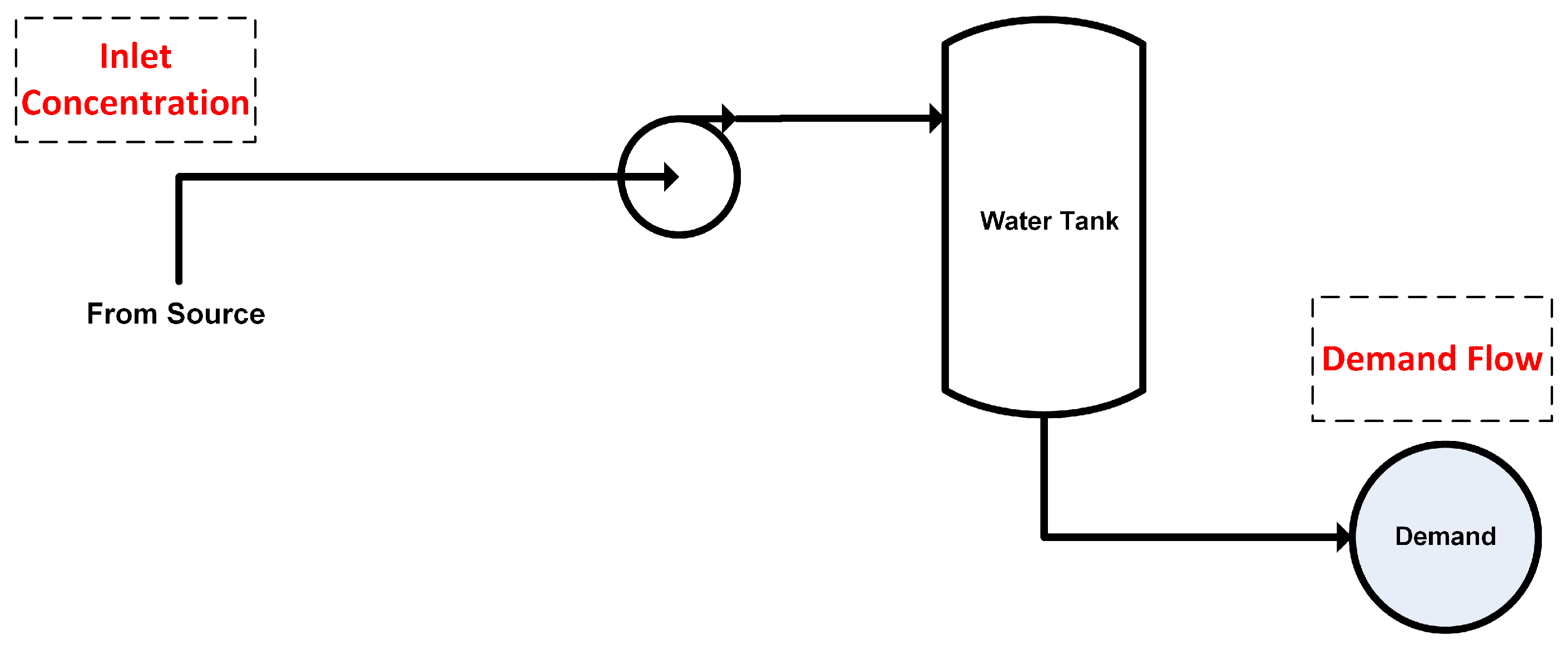
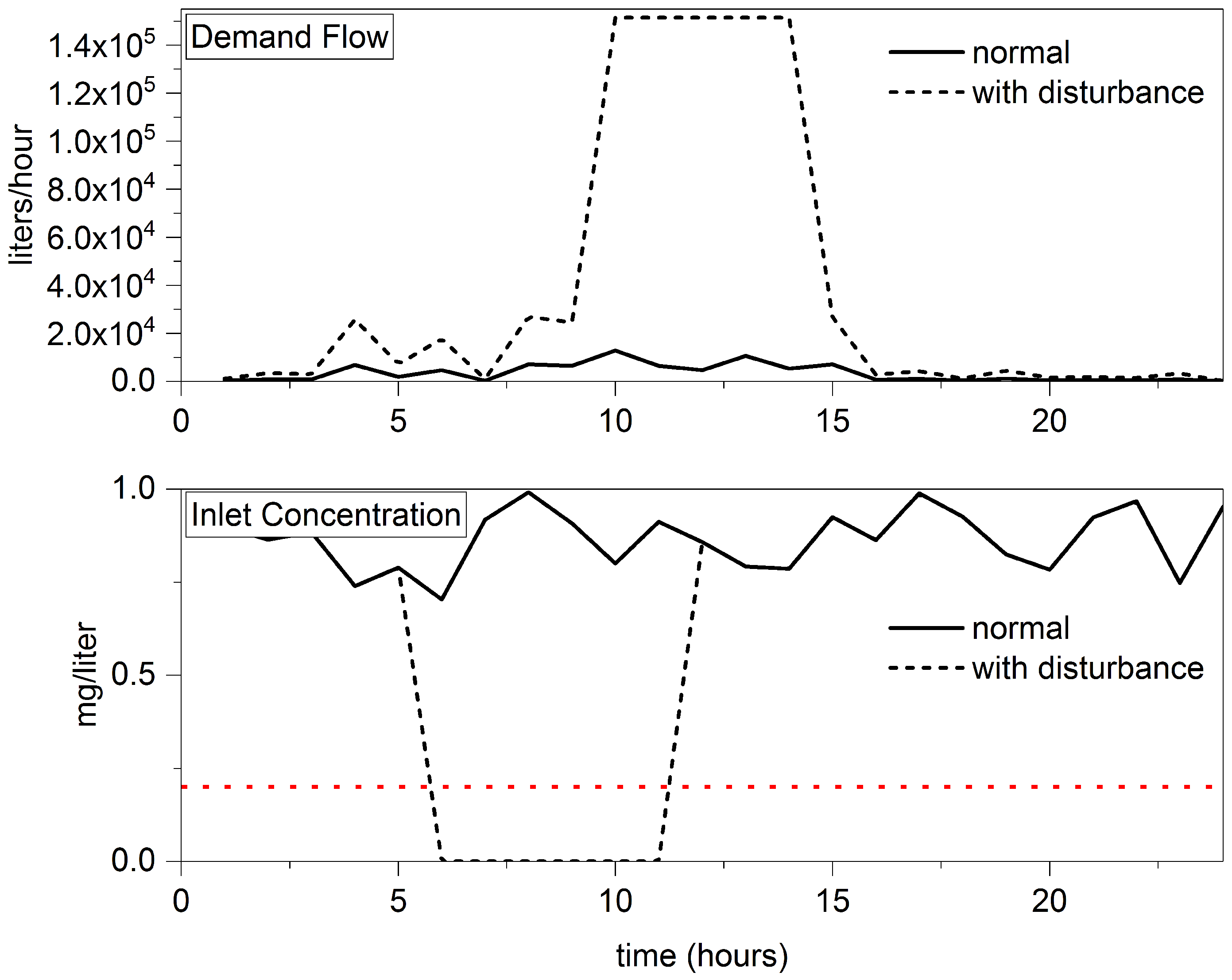
Large perturbations in municipal water systems are not unique to military bases, but the need to rapidly and accurately correct for disturbances is critical to base resiliency and safety. Resiliency on military bases is vulnerable to deficiencies in water systems created from a variety of disturbances: fires, terrorist activity, large leaks, or loss of chlorination at the inlet. Fires or large breaks in water lines caused by terrorist activity or other natural disasters, create an immediate and unpredicted demand that, without compensation, will quickly deplete water inventory. A large mechanized unit returning from training that requires intensive cleaning and maintenance could also put a similar stress on the water system. Figure 1 shows the physical location of perturbations used in this study at the inlet, or point where water is introduced to the system, and at the demand, which is modeled as a concentration of residential and industrial (military unit) consumers. Figure 2 shows plots of the relative disturbances. This study simulates a disturbance on demand, similar to the ones mentioned above, in the middle of the day when demand is already high. In the event of an extensive demand event, the flow of water required in the system would look more like the disturbance line in the upper plot of Figure 2. The line labeled “normal" depicts a standard day without excessive disturbances and a pattern of use that supports both residential and military operational needs. Typical system inlet chlorine concentration in this study ranges from 0.7–1.0 mg/L. The lower plot of Figure 2 shows a substantial disturbance on inlet concentration that, if not compensated for, would degrade water quality throughout the system and require extensive flushing that creates wasted water and energy. Such an event is a risk to the overall resiliency and security of base operations. Although these perturbations are only a fraction of the possibilities, they were chosen for this study to show the rigor of the proposed model predictive control (MPC) framework because they are large and occur when the system is under the most stress.
1.1. Motivation and Scope
The cost of providing potable water is mostly sensitive to tank water level. Tank water level does drive cost in most, if not all, water systems because pumping water into the system is the only manipulated variable (MV) available. When chlorine concentration decreases below the minimum level because of residence time or a disturbance on inlet concentration, the only MV to manipulate in water systems to increase the controlled variable (CV), or chlorine concentration at demand, c, is pumping flow, q. Especially when disturbances are excessive, a possibility on military bases, manipulating q as the only MV to change c will inevitably lead to excess water introduced into the system. The implication of introducing water in excess of demand is that it will most likely be wasted, or purged, after the chlorine concentration descends below the minimum level allowed by law. An alternate framework that will specifically target the prospect of disturbance variables (DV) of inlet concentration and demand while meeting the goals of the optimization layer is introduced here. The objectives of this work are to: (1) implement local regulatory control loops for tank water level (feedback) and inlet concentration (feedforward), (2) develop a nonlinear multi-input multi-output (MIMO) nonlinear model predictive controller (NMPC) to regulate the CVs with adequate MVs, (3) compare the performance of the MIMO MPC controller to regulatory control alone, (4) integrate chlorine injection as a manipulated variable, and (5) demonstrate the effectiveness of feedforward control on large scale disturbance rejection while minimizing cost and tank water level.
This work proposes a MPC supervisory layer, depicted in Figure 3, to minimize the impact of large, unpredicted disturbances while maintaining the strict constraints and resiliency requirements of military water systems. MPC is a tool used effectively in various process applications throughout the manufacturing and chemical industries [1]. If a reasonably accurate model is available, MPC is a suitable choice to provide supervisory control over processes like water networks where multiple inputs and outputs exist and strict inequality constraints must be met. Previous work by the authors demonstrates accurate nonlinear modeling of military water systems based on the work of Rossman et al. [2,3]. MPC implemented in this work will solve an optimal control problem under constraints with a specified prediction and control horizon. The controller will calculate control moves over the entire control horizon, but only implement the first move before repeating at the next time interval. At each time interval after implementing the first control move, the controller is providing inputs to change the trajectory of the controlled variables to their desired set points [4]. This work’s goal is to demonstrate the effective use of MPC on a military water system to reduce cost, water use, and ensure sufficient water inventory is maintained to establish resiliency in the system during times of stress on the system (large, unpredicted disturbances).
1.2. Literature Review
Led mainly by Mietek Brdys over the past two decades, a relatively small number of researchers have attempted to model and implement MPC on municipal water systems. MPC was successfully applied originally to minimize the cost of pumping [5,6,7,8]. Others took a more general approach using MPC, gaining good optimization and control of water quality and quantity in municipal systems as a whole [9,10,11,12,13,14]. An excellent feature article was published in 2002 providing an overview of feedback control as it applies to water quality [15]. A couple of key papers expand on the application of MPC to water systems by making improvements to the controllers or reducing uncertainty in the algorithms [16,17,18].
Even fewer researchers have used feedforward compensation in efforts to control water networks. The literature shows that the only mention of feedforward control action implemented with model predictive control in water networks is by Sandison [19]. Sandison implemented feedforward compensation on single loop systems with good results, but it is unclear how well the framework would perform under the stress of large inlet disturbances.
A knowledge gap exists in the literature in three areas that will be addressed here: (1) NMPC for the reduction of system volume and storage holdup, (2) feedforward integration to minimize disturbances, and (3) applying NMPC to reduce cost, electricity consumption and increase system resiliency under the unique constraints of military water systems.
2. Research Methods
2.1. System Identification
There are two models employed in this work. The dynamic nonlinear process model used in the real time optimization block of Figure 3 is outlined as [2,3]:
where chlorine concentration in the pipe bulk flow at time t, in pipe section k, and pipe segment i; volumetric flow rate; cross sectional area of specific pipe sections. The term on the left side of Equation (1) represents the change in chlorine concentration in pipe segments throughout the water distribution network with respect to time. The first term on the right describes the change in concentration axially along the length of each pipe segment, multiplied by the quotient of volumetric flow rate and cross sectional pipe area. It is this term that introduces nonlinear behavior to the model as the flow rate and concentration are changing simultaneously. The second term on the right describes the reaction kinetics multiplied by the chlorine concentration. represents the reaction kinetics of chlorine degradation as a function of time and temperature, outlined by Rossman et al. [2]. Further details regarding this model can be found in previous work by James et al. [3]. A series of perturbations were then used with this model and outputs were measured to generate a simpler model for control that would be both efficient and accurate.
A multi-input, multi-output (MIMO) transfer function model was identified to accurately predict tank water level, L, and chlorine concentration at demand, c as a function of four inputs: (1) pumping action, (2) chlorine injection, (3) demand flow, and (4) inlet chlorine concentration and be employed for control purposes in this work. Step changes were made in each input in the aforementioned distributed model and the results of the system identification is depicted in Table 1.
The System Identification ToolboxTM in the MATLAB® software package (version R2017A, MathWorks, Natick, MA, USA) was used to identify transfer function models for each input/output combination. The relationship between each input and output was captured with at least a 74% fit, so the transfer function models were used in the development of a model predictive controller. The positive result of system identification is evident in Figure 4 where the distributed model and transfer function model describing tank level are very similar. A common practice in MPC development is to use step-response models instead of transfer functions, particularly in highly nonlinear cases [4]. This work did not yet explore the use of step-response modeling to describe the water system and, to the author’s knowledge, this technique has not been used in water system modeling.
2.2. Nonlinear Disturbance Controller Development
If a disturbance can be detected before it enters the process and the process model is sufficiently accurate, feedforward MPC can often provide better disturbance rejection than feedback MPC alone [20]. Most feedforward systems use feedback trim as a means to compensate for errors in modeling and feedforward control discrepancies. However, self-regulating systems that do not require set point tracking, like chlorine concentration in water systems in the presence of large disturbances, can be controlled adequately with feedforward control alone [21].
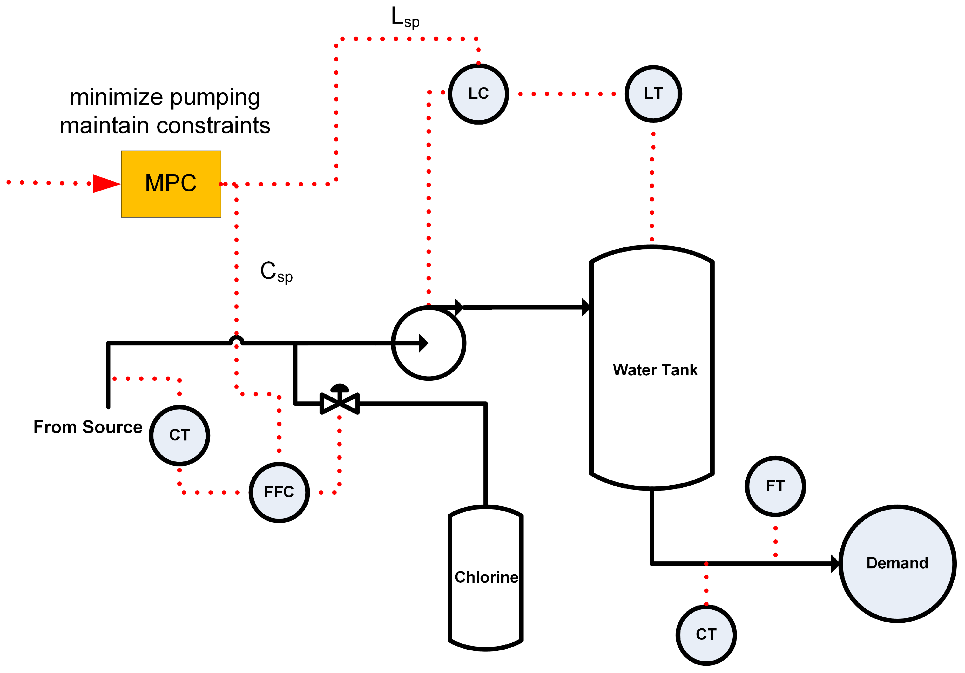
This section outlines a NMPC based on a dynamic system model, illustrated by the process flowsheet in Figure 5 and the block diagrams in Figure 6, Figure 7 and Figure 8 that utilize two control loops to reject large process disturbances: (1) a feedback loop that rejects large disturbances on demand, maintains tank holdup above the minimum resiliency constraint, and minimizes the amount of water inventory on hand and (2) a feedforward loop that rejects large disturbances on inlet concentration to ensure that downstream chlorine concentration remains at acceptable levels.
The “control calcuations” block in Figure 6 is made up of the feedforward and feedback loops in Figure 7 and Figure 8. The optimization/scheduling layer provides set points to the control loops based on the model’s prediction and inputs on the system such as electricity prices, predicted demand, and inlet concentration. Furthermore, the optimization/scheduling layer provides predictive pump scheduling for the system, which is shown as an input to the feedback control loop in Figure 8.
The nonlinear nature of the model requires that the NMPC problem be formulated using a two-phase approach: estimation phase and control move calculation phase [20]. The estimation phase is stated here as a nonlinear sub-problem:
subject to:
where represents the controlled states, namely tank water level and chlorine concentration at demand, and represent estimated system parameters and disturbances, respectively, and and represent predicted and measured output, respectively. The prediction horizon, P, is 24 h in this study due to the accessibility of day ahead electricity pricing.
Similar to a linear case, the control move calculation phase is used to calculate the current control action, , plus additional control action and minimize the calculations over the control horizon, M. This work uses two control loops to calculate control moves: a feedback loop to control tank water holdup and a feedforward loop to control chlorine injection in an effort to minimize the effects of large disturbances on inlet chlorine concentration. The feedback loop utilizes a simple proportional control method to allow for averaging level control. Proportional control is also adequate in this case because offset from the set point is allowed:
In Equation (4), represents the steady state value, is the scheduled pumping action passed from the optimization/scheduling layer, and is the proportional gain for the feedback loop [4]. The error, e is defined as:
where is either the tank level set point, or the inlet chlorine concentration set point, and is the measured corresponding output values. The feedforward portion of the control phase is treated as “perfect” feedforward control, where the control action is designed to keep the controlled variable exactly at the set point despite dynamic effects from the system [4]:
The dynamic effects of the transmitter and valve, represented by transfer functions and , respectively, are neglected in this study and then is estimated as a lead–lag unit accounting for process and disturbance dynamics, and , respectively. A lead–lag unit is used to estimate the dynamics of the disturbances and process and their effect on the control action. Attempting to use the transfer functions outlined in Table 1 leads to a physically unrealizable controller:
, , and are adjustable parameters in Equation (7). The adjustable parameters were tuned using the steps outlined in Seborg et al. [4]. Due to the dynamics in this system, offset is not a concern and was adjusted until a reasonable control response was achieved. The optimal value used for in this work was determined to be 0.35. and were set to zero while a trial and error approach was used to establish an appropriate value for . The controlled variable responds faster to the manipulated variable in this system due to its location upstream of the disturbance variable, so the heuristic approach of was used to set an initial value for these two parameters. and were then slightly fine tuned to .01 and .025, respectively, as the disturbance value was adjusted to establish the controller so that it would minimize large disturbances effectively. The controller action, , is then defined as multiplied by the disturbance in inlet chlorine concentration, :
The NMPC control law in Equations (2)–(8) is a multi-variable, proportional control law utilizing a receding horizon approach and a dynamic process model. It is based on predicted error generated by the optimization/scheduling layer shown in Figure 6. The controller tuning parameters are shown in Table 2. To ensure that the slowest dynamics in the system were adequately compensated for, this study used the settling time () of the demand chlorine concentration control response. It was determined to be 13 h. Heuristics outlined in Seborg et al. were then used to determine values for the control (M) and prediction (P) horizons in Equation (9) [4]. All outputs are weighted equally, so the diagonal elements () of the output weighting matrix () are assigned a value of unity:
3. Results
3.1. Averaging Level Control
The storage tanks in water systems are operated as surge tanks to not only damp out oscillations in the inlet stream, but to provide a constant and predictable pressure to customers. Where downstream flow rates change gradually, water levels can be maintained within specified upper and lower limits, and steady-state mass balances can be satisfied at all times, averaging level control is appropriate and is often employed successfully when conditions warrant [4,21].
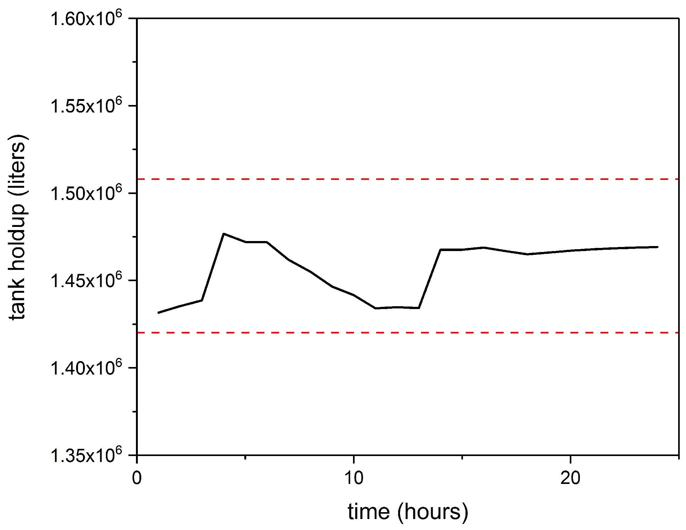
Using averaging level control in this system contributes greatly to the systems’ ability, guided by robust control and optimization, to minimize large disturbances. Figure 9 shows the results of averaging level control on the model system, giving the controller flexibility to hold inventory when predictions require it.
The NMPC controller described in the previous section was implemented using the General Algebraic Modeling System (GAMS) and the MATLAB Simulink environment. GAMS performed the optimization and scheduling of pumping action based on the system model. The remainder of this section is dedicated to presenting the results of this work.
3.2. Closed Loop Controller Response
Figure 10 shows the control action affecting tank water holdup under large disturbances. The controller provides an immediate and accurate response to a large demand load on the system beginning at hour eight and continuing to hour fifteen. Although there is approximately one hour of delay in the system’s reaction to the demand, the effect of the large demand on the CV is minimal and the critical tank holdup is maintained. The input curve at the top of Figure 10 shows two large control actions: (1) scheduled pumping during non-peak hours (night) that was completed to avoid pumping during the peak hours of the day and (2) un-scheduled pumping during peak hours due to closed-loop control attempting to maintain the system within constraints during a large disturbance event. When compared to closed-loop proportional control under the same conditions, MPC is the clear choice to ensure the effect of disturbances is minimized. Figure 10 shows the proportional controller recovering the system to the set point, but the response is delayed for approximately eight hours and it allows the tank holdup level to decrease well below the lower constraint of L. The military’s need for aggressive adherence to the lower constraint on tank holdup for resiliency purposes means that regulatory control alone is insufficient.
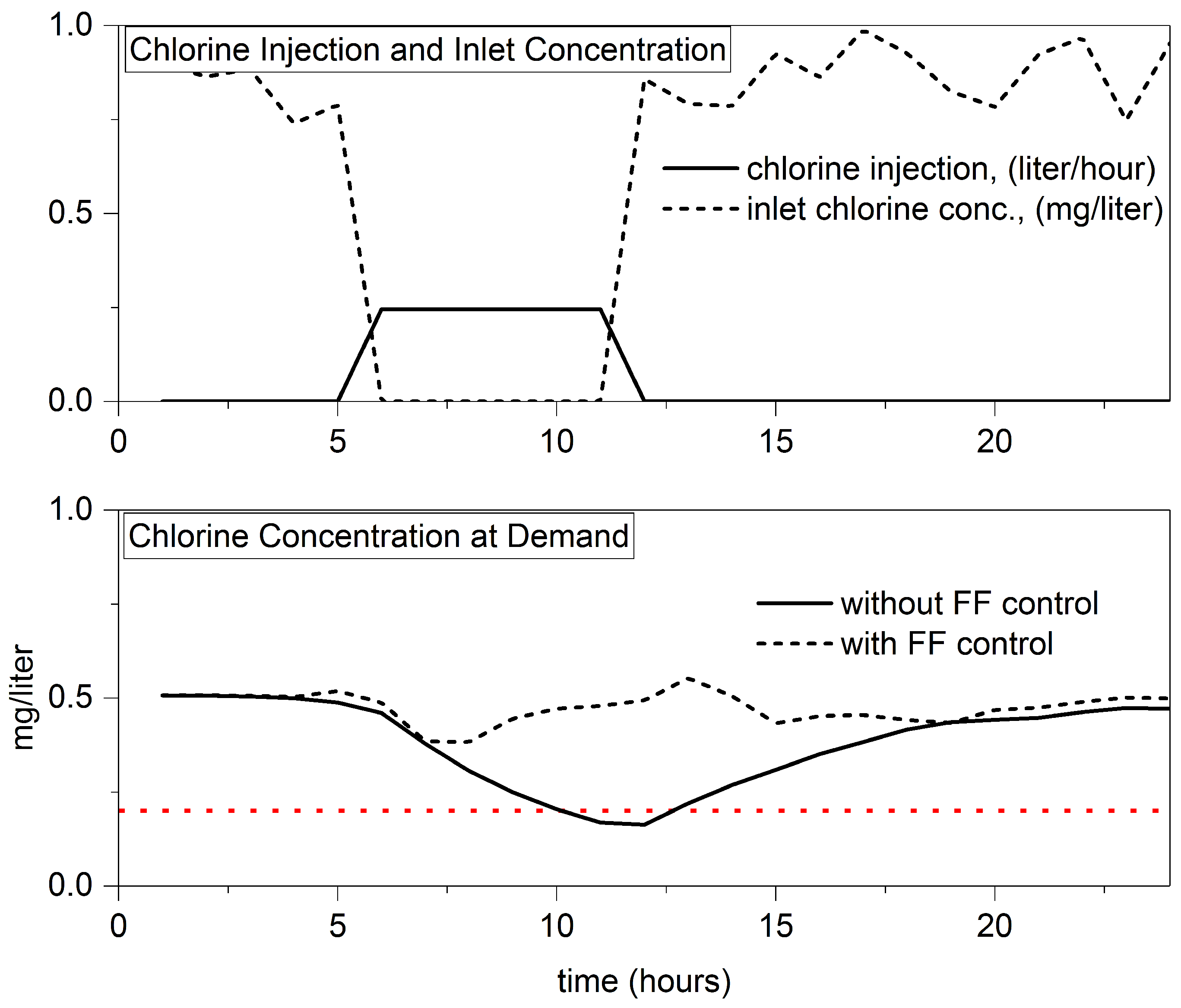
Large disturbances on inlet concentration pose a unique challenge to military water systems. Due to the size of water systems, the distance between the inlet and the CV of concern is usually extensive. Distance and chlorine reaction kinetics combine to create a time delay on the demand chlorine concentration. If a large disturbance on inlet concentration were to occur currently, the majority of the water system would be contaminated before the disturbance was detected. Feedforward control shown in Figure 11 demonstrates an effective solution to large disturbances. Because the disturbance is recognized immediately by the controller as well as the plant, control action begins to compensate immediately after the disturbance occurs. The CV continues to decrease for at least two hours after compensation due to the system time delay, but the CV remains well within constraints. Conversely, the CV decreases below the lower chlorine concentration constraint when model based control with feedforward action is not employed. Without feedforward control, the system time delay dominates, ensures that the concentration descends below the lower constraint, and spends at least twelve hours re-establishing the steady state.
While conserving water and electricity are motivations for this work, reducing costs to the military while maintaining resiliency receive priority when inefficiencies are concerned.
3.3. Robustness Analysis
Effective control systems are required to adequately counter process disturbances while also providing satisfactory performance for a wide range of process conditions and a reasonable degree of model inaccuracy [4]. The ability to control the system under a variety of conditions is known as robustness. Figure 10, Figure 11, Figure 12 and Figure 13 shown earlier in this section demonstrate the performance of the control hierarchy in this work. Analysis was conducted on the control hierarchy to determine if it was effective beyond the scope of the figures earlier in this section. Figure 14 shows great control system response in terms of its ability to rapidly and smoothly compensate for a range of unpredicted demand events. The demand events are arrayed between a normal operation status with no large demand events and a disturbance to the system of 151,000 L. In all cases, resiliency within the system is shown by a rapid response and the ability to maintain the tank water level well above the lower safety threshold of 1,400,000 L.
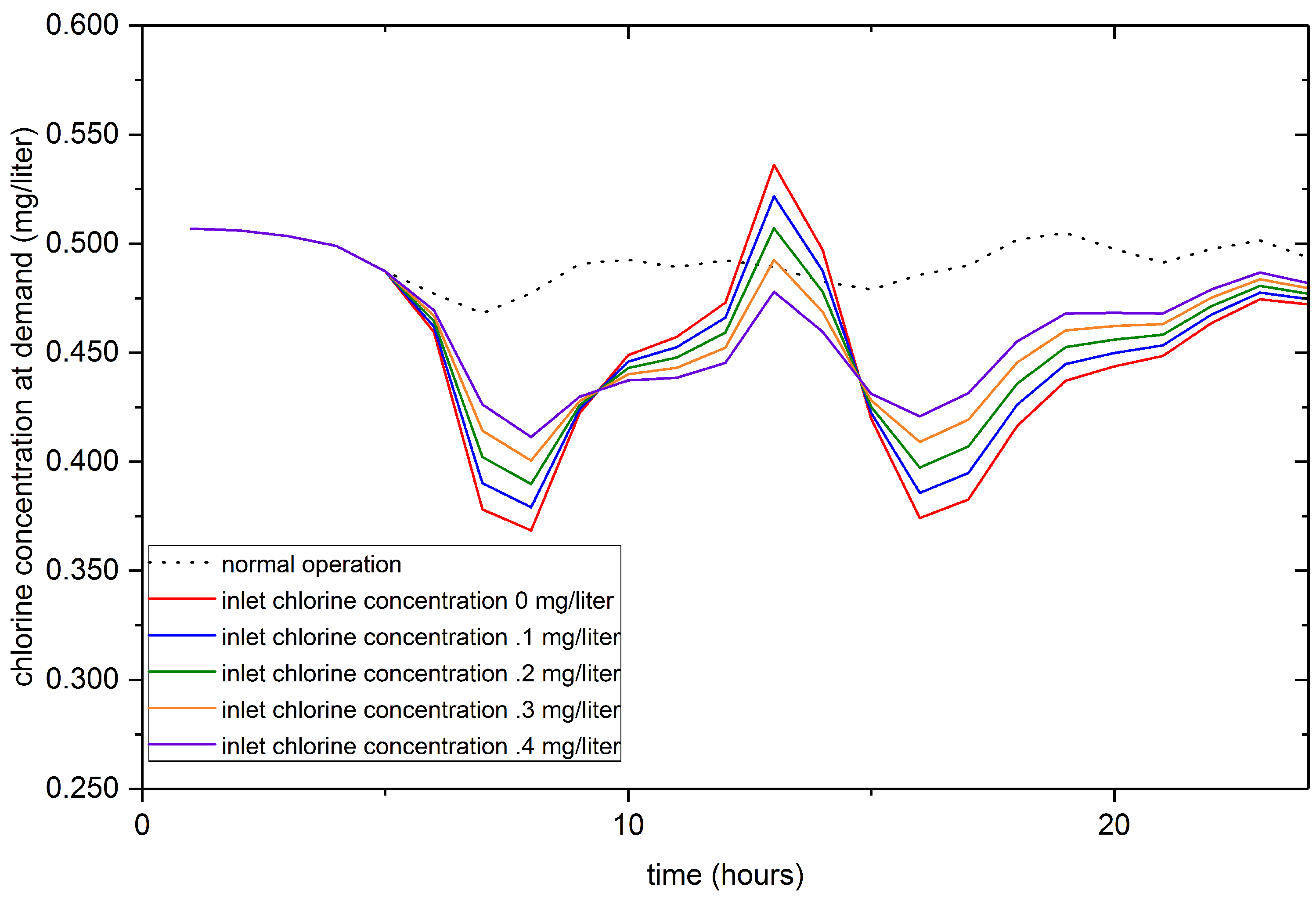
Figure 15 demonstrates, with respect to the controlled variable of demand chlorine concentration, that the control hierarchy is capable of efficiently handling a wide range of disturbances. Under normal conditions in this model system, an inlet concentration that ranges from 0.7 mg/L to 1.0 mg/L will lead to a demand chlorine concentration of approximately 0.5 mg/L. If large disturbances on inlet chlorine concentration were allowed to persist without compensation, contamination and water waste will result. Figure 15 shows that the control system will inject chlorine to adequately compensate for substantial losses in inlet chlorine ranging from 0 mg/liter to 0.4 mg/L. Each disturbance is smoothly compensated for and the overall result is the entire model water system maintaining a chlorine concentration above the minimum safe level of 0.2 mg/L.
4. Discussion
Since the majority of the cost of providing potable water to installations is related to pumping water to fill tanks, it follows that any efforts to minimize cost should begin there. As shown in Figure 12, the MPC framework outlined earlier in this paper attempts to pump in a pattern that avoids the more expensive times of the day based on day ahead electricity pricing. Figure 12 shows the action of MPC with and without large disturbances present. Without disturbances, the controller will ensure that pumping is accomplished in the most inexpensive manner possible and will only pump during the unfavorable hours of the day if it needs to in order to maintain critical system constraints. Safety and resiliency are prioritized by the controller. Regulatory control alone will also effectively manage tank holdup in the absence of disturbances, but does not discriminate against higher prices in the afternoon, leading to excessive cost. Because of its predictive nature, MPC has the effect of having water inventory on hand when large disturbances occur that allow it to respond in a more efficient and inexpensive manner. Regulatory control alone with no predictive capability is at a disadvantage and does not perform as well because it did not store an additional amount of inventory during the more inexpensive times of the day. Figure 13 shows the cost comparison of regulatory control and MPC with no disturbances present. A 12% decrease in cost is realized when MPC is implemented. This decrease is realized because the controller manipulates the pumping action based on the cost of electricity and regulatory control does not.
5. Conclusions
In conclusion, large disturbances within military water systems can be adequately controlled using nonlinear model predictive control. Due to distance, time delays, time scales, and reaction kinetics, multiple types of control (feedback, feedforward, etc.) should be employed in the regulatory layer to compensate for disturbances effectively while maintaining constraints for safety and resiliency. Water system modeling is hindered by the existence of different time scales of phenomena within the system. The solution of this controller follows the process control hierarchical structure in Figure 3, employing the regulatory control layer to manage the fast dynamics of the system while the supervisory controller developed in this paper effectively managed the slow dynamics [22]. The NMPC framework outlined lowers costs and reduces waste, while improving resiliency and safety.
Acknowledgments
This work was funded by the United States Army as part of the Advanced Civil Schooling (ACS) program.
Author Contributions
Corey M. James, Michael E. Webber, and Thomas F. Edgar conceived the idea to place rigorous controls on military water systems, while Corey M. James designed and wrote the code to implement control on the system. Corey M. James, Michael E. Webber, and Thomas F. Edgar analyzed the data and Corey M. James authored the paper. Michael E. Webber and Thomas F. Edgar helped review the paper.
Conflicts of Interest
The authors declare no conflict of interest. The founding sponsors had no role in the design of the study; in the collection, analyses, or interpretation of data; in the writing of the manuscript, and in the decision to publish the results.
References
- Qin, S.J.; Badgwell, T.A. A survey of industrial model predictive control technology. Control Eng. Pract. 2003, 11, 733–764. [Google Scholar] [CrossRef]
- Rossman, L.A.; Clark, R.M.; Grayman, W.M. Modeling chlorine residuals in drinking-water distribution systems. J. Environ. Eng. 1994, 120, 803–820. [Google Scholar] [CrossRef]
- James, C. Reducing the Cost of Operational Water on Military Bases Through Modeling, Optimization, and Control. Ph.D. Thesis, The University of Texas at Austin, Austin, TX, USA, 2017. [Google Scholar]
- Seborg, D.E.; Mellichamp, D.A.; Edgar, T.F.; Doyle, F.J., III. Process Dynamics and Control; John Wiley & Sons: Hoboken, NJ, USA, 2016. [Google Scholar]
- Ormsbee, L.; Reddy, L.; Chase, D. Comparison of Three Nonlinear Control Algorithms for the Optimal Operation of Water Supply Pumping Systems; Integrated Computer Applications in Water Supply (Vol. 1); John Wiley & Sons, Inc.: Hoboken, NJ, USA, 1994; pp. 259–271. [Google Scholar]
- Ormsbee, L.E.; Lansey, K.E. Optimal control of water supply pumping systems. J. Water Resour. Plan. Manag. 1994, 120. [Google Scholar] [CrossRef]
- Van Staden, A.J.; Zhang, J.; Xia, X. A model predictive control strategy for load shifting in a water pumping scheme with maximum demand charges. Appl. Energy 2011, 88, 4785–4794. [Google Scholar] [CrossRef]
- Yu, G.; Powell, R.; Sterling, M. Optimized pump scheduling in water distribution systems. J. Optim. Theory Appl. 1994, 83, 463–488. [Google Scholar] [CrossRef]
- Duzinkiewicz, K.; Brdys, M.; Chang, T. Hierarchical model predictive control of integrated quality and quantity in drinking water distribution systems. Urban Water J. 2005, 2, 125–137. [Google Scholar] [CrossRef]
- Brdys, M.A.; Chang, T.; Duzinkiewicz, K.; Chotkowski, W. Hierarchical control of integrated quality and quantity in water distribution systems. In Proceedings of the ASCE 2000 Joint Conference on Water Resources Engineering and Water Resources Planning and Management, Minneapolis, MN, USA, 30 July–2 August 2000. [Google Scholar]
- Chang, T.; Brdys, M.; Duzinkiewicz, K. Decentralized robust model predictive control of chlorine residuals in drinking water distribution systems. In Proceedings of the World Water and Environmental Resources Congress, World Water and Environmental Resources Congress and Related Symposia, Philadelphi, PA, USA, 23–26 June 2004; pp. 23–26. [Google Scholar]
- Wang, J.; Brdys, M.A. Optimal operation of water distribution systems under full range of operating scenarios. In Proceedings of the 6th UKACC International Control Conference, Glasgow, UK, 30 August–1 September 2006. [Google Scholar]
- Drewa, M.; Brdys, M.; Ciminski, A. Model predictive control of integrated quantity and quality in drinking water distribution systems. In Proceedings of the 8th International IFAC Symposium on Dynamics and Control of Process Systems, Cancún, Mexico, 6–8 June 2007. [Google Scholar]
- Brdys, M.; Chang, T.; Duzinkiewicz, K. Intelligent model predictive control of chlorine residuals in water distribution systems. In Proceedings of the ASCE Water Resource Engineering and Water Resources Planning and Management, Orlando, FL, USA, 20–24 May 2001; pp. 391–401. [Google Scholar]
- Polycarpou, M.M.; Uber, J.G.; Wang, Z.; Shang, F.; Brdys, M. Feedback control of water quality. IEEE Control Syst. 2002, 22, 68–87. [Google Scholar] [CrossRef]
- Trawicki, D.; Duzinkiewicz, K.; Brdys, M. Optimising model predictive controller for hierarchical control of integrated quality and quantity in drinking water distribution systems. In Proceedings of the IFAC I International Conference on Technology, Automation and Control of Wastewater Systems-TiASWiK’02, Gdansk-Sobieszewo, Poland, 19–21 June 2002; pp. 19–21. [Google Scholar]
- Chang, T.; Brdys, M.; Duzinkiewicz, K. Quantifying uncertainties for chlorine residual control in drinking water distribution systems. Proc. ASCE World Water Environm. Resour. 2003, 64, 28–37. [Google Scholar]
- Wang, Y.; Puig, V.; Cembrano, G. Non-linear economic model predictive control of water distribution networks. J. Process Control 2017, 56, 23–34. [Google Scholar] [CrossRef]
- Sandison, J. Controlling chlorination in drinking water: Water and waste water. IMIESA 2006, 31, 32–37. [Google Scholar]
- Brosilow, C.; Joseph, B. Techniques of Model-Based Control; Prentice Hall Professional: Upper Saddle River, NJ, USA, 2002. [Google Scholar]
- Shinskey, F.G. Process Control Systems: Application, Design and Tuning; McGraw-Hill, Inc.: London, UK, 1990. [Google Scholar]
- Touretzky, C.R.; Baldea, M. Nonlinear model predictive control of energy-integrated process systems. Syst. Control Lett. 2013, 62, 723–731. [Google Scholar]
Figure 1.
Locations of perturbations used in this study for demand and inlet concentration to demonstrate the effectiveness of model predictive control (MPC).
Figure 1.
Locations of perturbations used in this study for demand and inlet concentration to demonstrate the effectiveness of model predictive control (MPC).

Figure 2.
Simulated disturbances used in this study for demand and inlet concentration. The red dotted line at 0.2 mg/L signifies the lower limit of system chlorine concentration allowed to ensure a potable water supply.
Figure 2.
Simulated disturbances used in this study for demand and inlet concentration. The red dotted line at 0.2 mg/L signifies the lower limit of system chlorine concentration allowed to ensure a potable water supply.

Figure 3.
Hierarchy of process control in this work [4].
Figure 3.
Hierarchy of process control in this work [4].
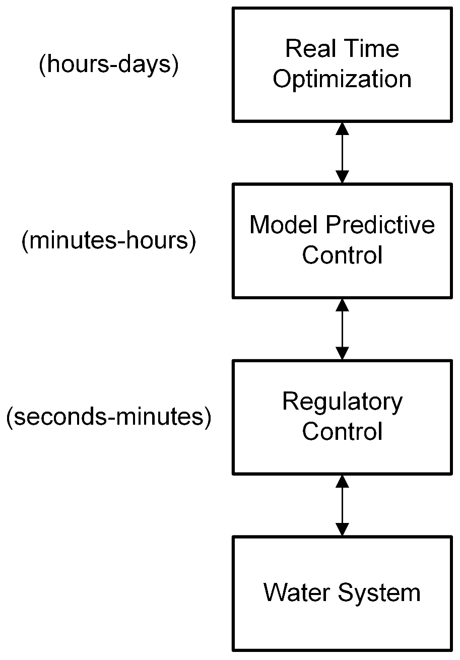
Figure 4.
Comparison of tank water volume predicted by the distributed modeling (solid) and the transfer function models shown in Table 1 (dashed). The solid red line, referenced to the right y-axis, depicts scheduled and unscheduled pumping by the controller.
Figure 4.
Comparison of tank water volume predicted by the distributed modeling (solid) and the transfer function models shown in Table 1 (dashed). The solid red line, referenced to the right y-axis, depicts scheduled and unscheduled pumping by the controller.
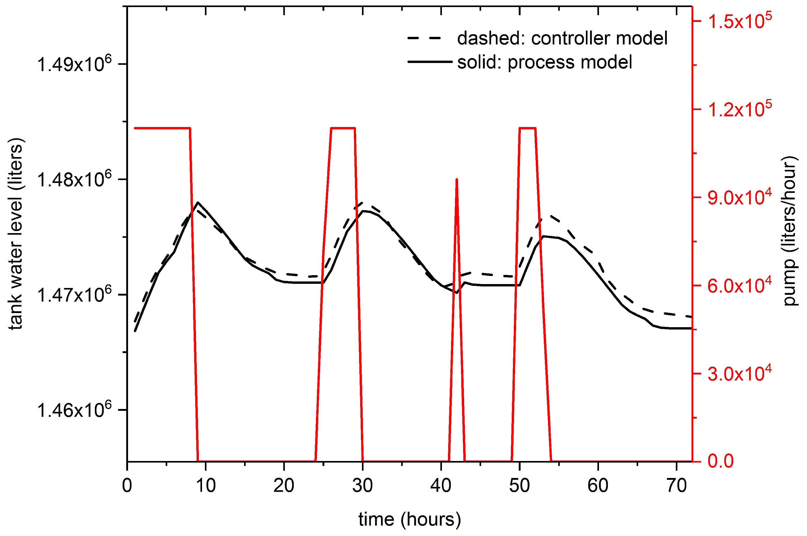
Figure 5.
MPC framework with feedforward and feedback structure for disturbance compensation. and are level and feedforward controllers, respectively. , , and are transmitters for level, flow, and concentration, respectively. is the tank level set point and is the inlet chlorine concentration set point.

Figure 6.
Block diagram for model predictive control with feedforward disturbance compensation, modified from Seborg et al. [4].
Figure 6.
Block diagram for model predictive control with feedforward disturbance compensation, modified from Seborg et al. [4].
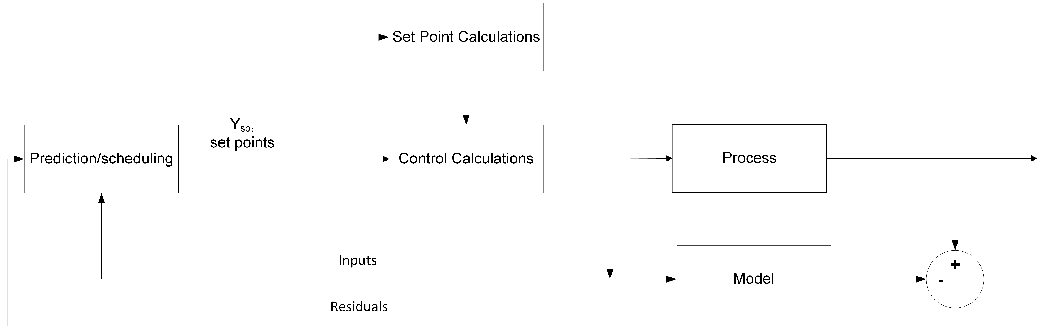
Figure 7.
Block diagram for feedforward control. The control action is a portion of the “control calculations” block in Figure 6., modified from Seborg et al. [4].
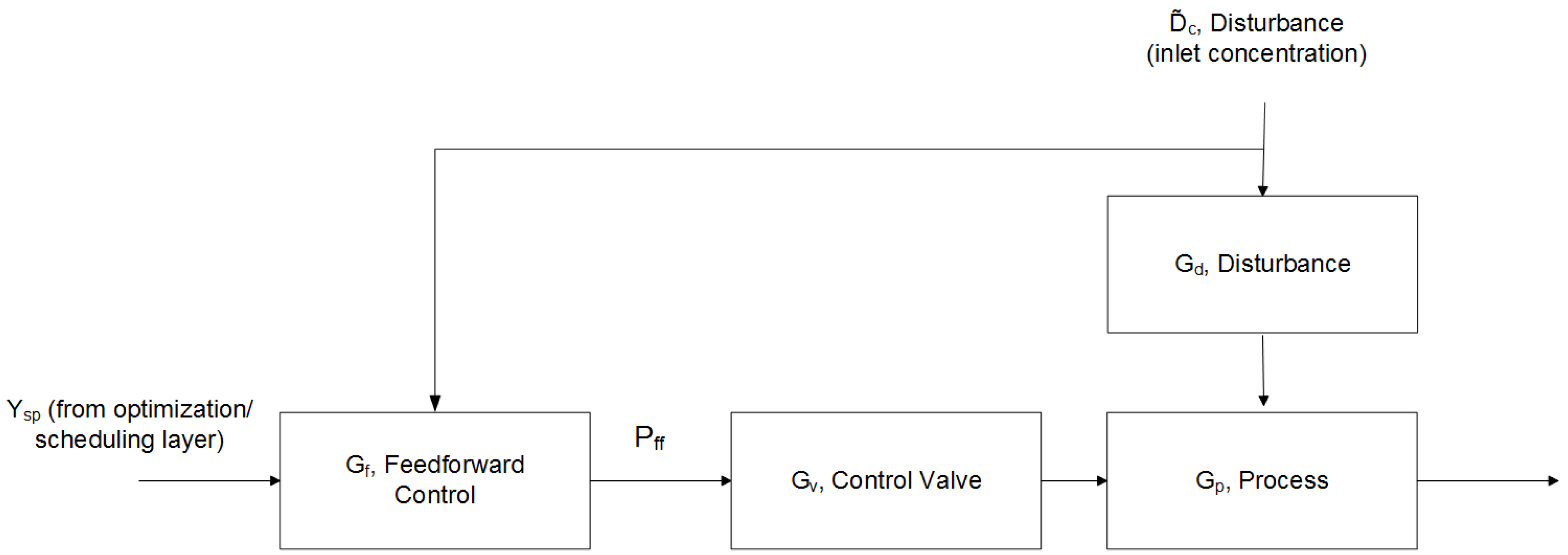
Figure 8.
Block diagram for feedback control with included planned pumping from the optimization/scheduling layer. The control action is a portion of the “control calculations” block in Figure 6, modified from Seborg et al. [4].
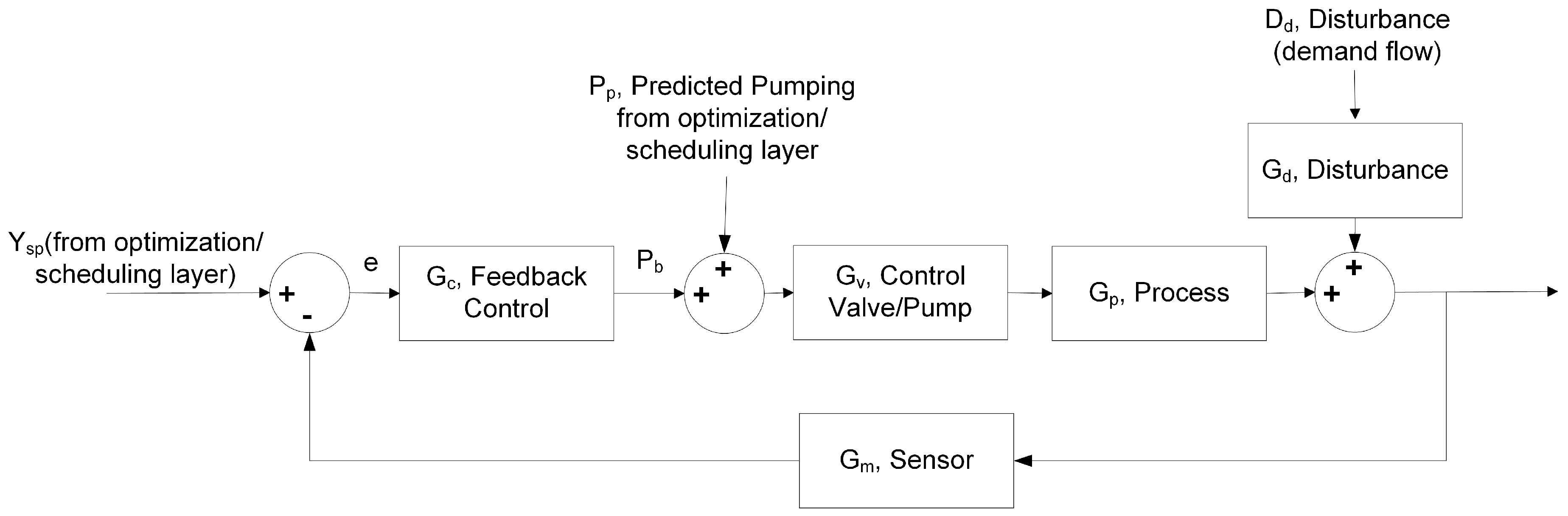
Figure 9.
Average level control of tank holdup. Red dotted lines represent upper and lower constraints on tank holdup.
Figure 9.
Average level control of tank holdup. Red dotted lines represent upper and lower constraints on tank holdup.

Figure 10.
Controller action to minimize disturbance on tank holdup. In the bottom plot, MPC is compared to proportional control on tank holdup under the same conditions.
Figure 10.
Controller action to minimize disturbance on tank holdup. In the bottom plot, MPC is compared to proportional control on tank holdup under the same conditions.
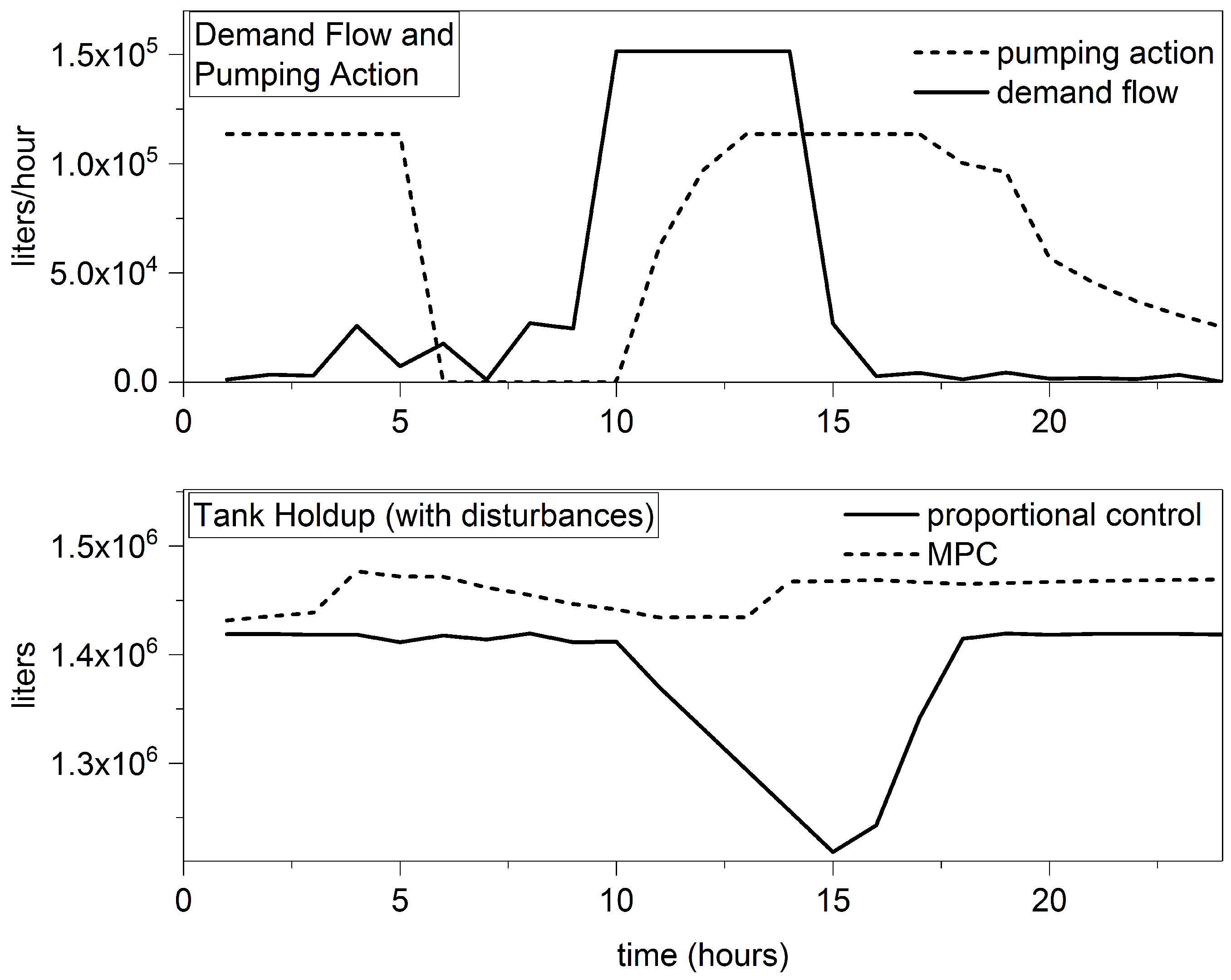
Figure 11.
Feedforward control response to large disturbances on inlet chlorine concentration and the effect on demand chlorine concentration.
Figure 11.
Feedforward control response to large disturbances on inlet chlorine concentration and the effect on demand chlorine concentration.

Figure 12.
Comparison of pumping controlled by proportional control alone and model predictive control and how those strategies react to large disturbances.
Figure 12.
Comparison of pumping controlled by proportional control alone and model predictive control and how those strategies react to large disturbances.
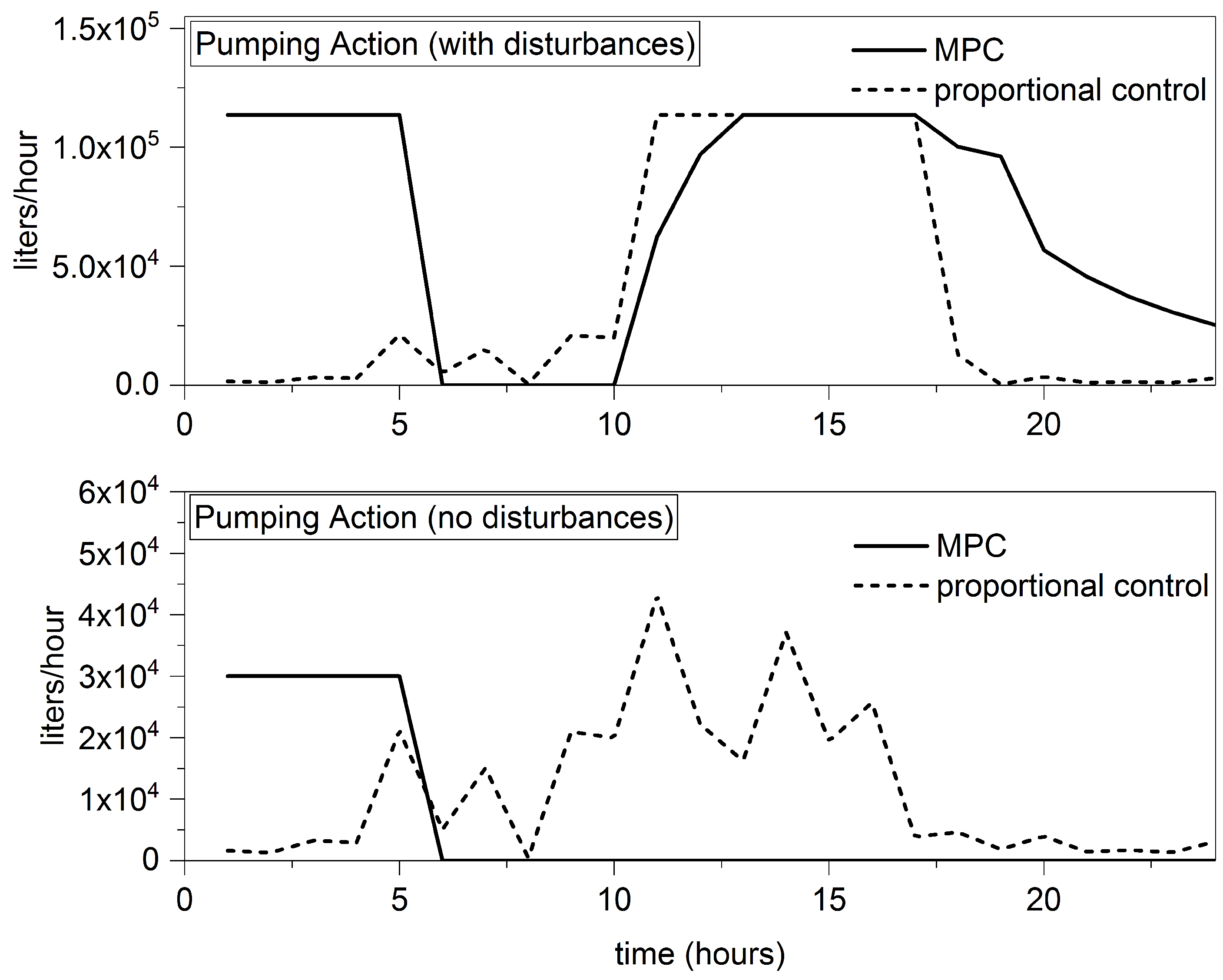
Figure 13.
Cost of pumping over a 24 h period when proportional control and model predictive control are employed on the water system.
Figure 13.
Cost of pumping over a 24 h period when proportional control and model predictive control are employed on the water system.
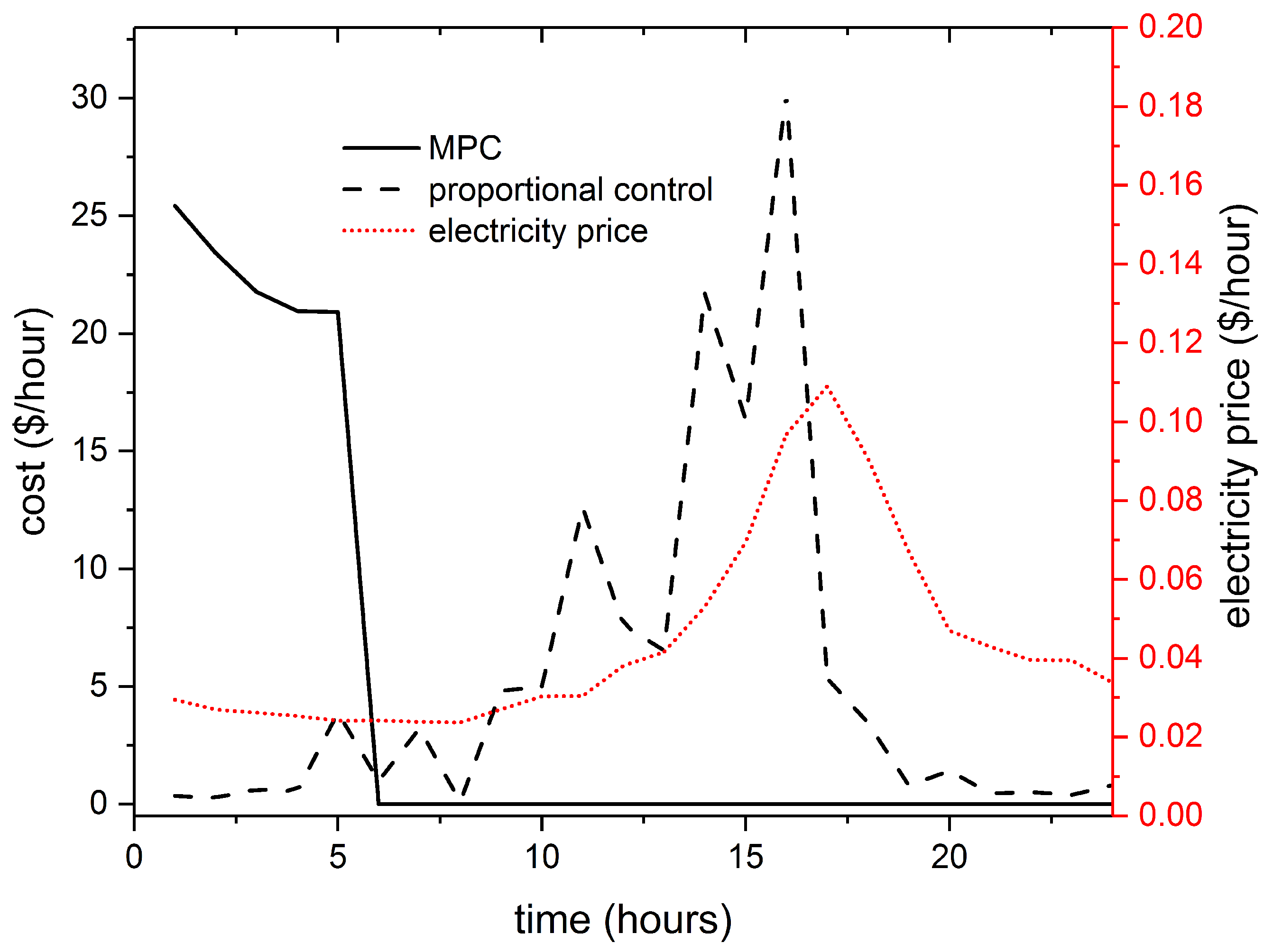
Figure 14.
Controller response to a range of demand disturbances in order to maintain tank water level.
Figure 14.
Controller response to a range of demand disturbances in order to maintain tank water level.
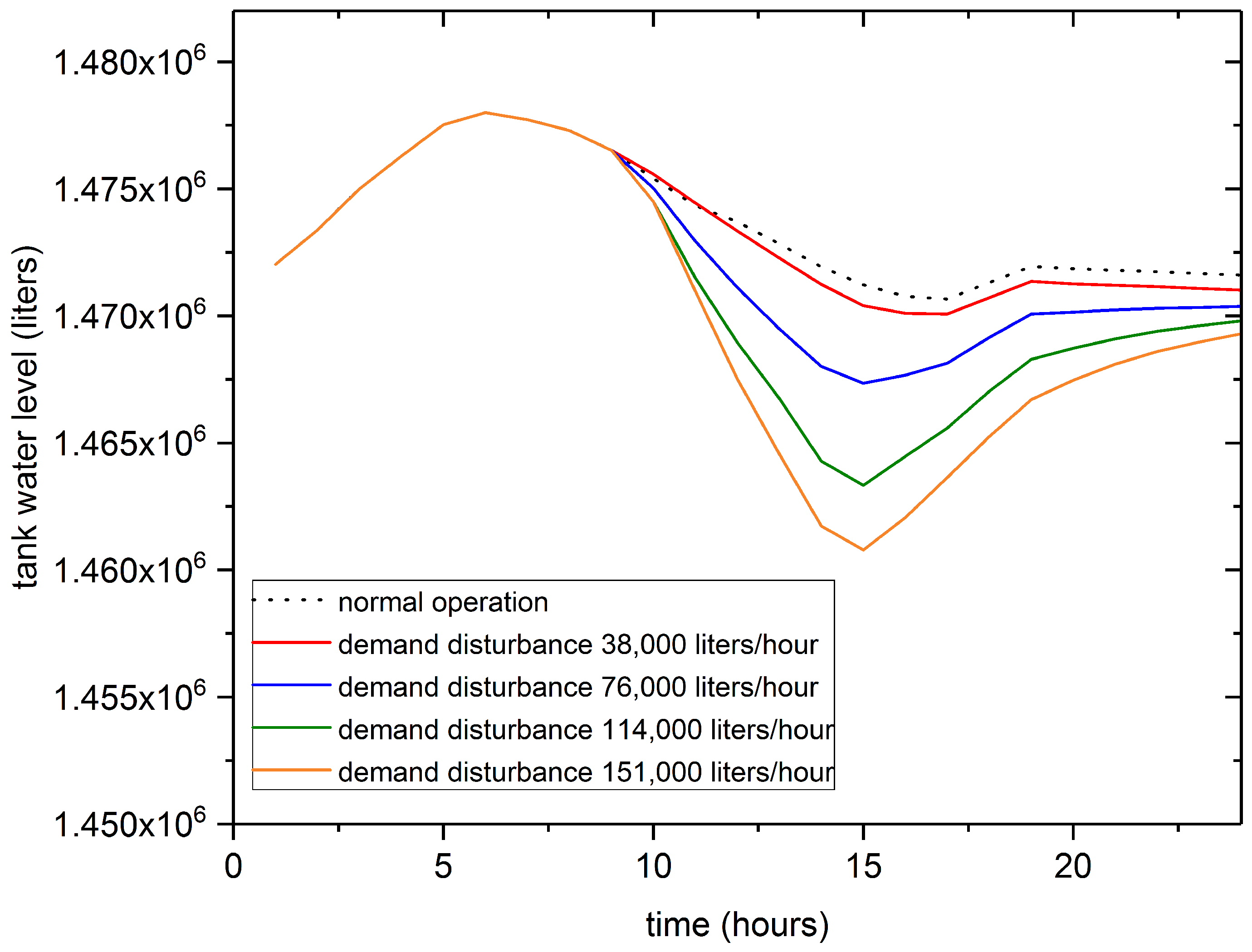
Figure 15.
Controller response to a range of inlet chlorine concentration disturbances to ensure downstream demand chlorine concentration remains above the safe limit of 0.2 mg/L.
Figure 15.
Controller response to a range of inlet chlorine concentration disturbances to ensure downstream demand chlorine concentration remains above the safe limit of 0.2 mg/L.


Table 1.
Individual step-response models for the identified water system in Figure 5 with four inputs and two outputs. The two blank plots represent no influence from inputs on CVs (CV: controlled variable, MV: manipulated variable, DV: disturbance variables).
Table 1.
Individual step-response models for the identified water system in Figure 5 with four inputs and two outputs. The two blank plots represent no influence from inputs on CVs (CV: controlled variable, MV: manipulated variable, DV: disturbance variables).
| Tank Holdup, CV | Demand Chlorine Concentration, CV | |
|---|---|---|
| Pump, MV | ||
| Chlorine Injection, MV | ||
| Demand, DV | ||
| Initial Concentration, DV |
Table 2.
MPC model parameters (MPC: model predictive control).
| Parameter | Value | Units |
|---|---|---|
| M | 5 | h |
| P | 24 | h |
| 1 | ||
| 0 | L/h | |
| 3.79 | L/h | |
| 0 | L/h | |
| 113,562 | L/h | |
| −0.35 | mg/L2 | |
| 15 | h |
© 2017 by the authors. Licensee MDPI, Basel, Switzerland. This article is an open access article distributed under the terms and conditions of the Creative Commons Attribution (CC BY) license (http://creativecommons.org/licenses/by/4.0/).
Share and Cite
MDPI and ACS Style
James, C.M.; Webber, M.E.; Edgar, T.F. Minimizing the Effect of Substantial Perturbations in Military Water Systems for Increased Resilience and Efficiency. Processes 2017, 5, 60. https://doi.org/10.3390/pr5040060
AMA Style
James CM, Webber ME, Edgar TF. Minimizing the Effect of Substantial Perturbations in Military Water Systems for Increased Resilience and Efficiency. Processes. 2017; 5(4):60. https://doi.org/10.3390/pr5040060
Chicago/Turabian StyleJames, Corey M., Michael E. Webber, and Thomas F. Edgar. 2017. "Minimizing the Effect of Substantial Perturbations in Military Water Systems for Increased Resilience and Efficiency" Processes 5, no. 4: 60. https://doi.org/10.3390/pr5040060
Note that from the first issue of 2016, this journal uses article numbers instead of page numbers. See further details here.