Improving Bioenergy Crops through Dynamic Metabolic Modeling

The Wallace H. Coulter Department of Biomedical Engineering, Georgia Institute of Technology and Emory University, 950 Atlantic Drive, Atlanta, GA 30332-2000, USA
*
Author to whom correspondence should be addressed.
Processes 2017, 5(4), 61; https://doi.org/10.3390/pr5040061
Submission received: 4 September 2017
/
Revised: 3 October 2017
/
Accepted: 7 October 2017
/
Published: 18 October 2017
(This article belongs to the Special Issue Biological Networks)
Abstract
:Enormous advances in genetics and metabolic engineering have made it possible, in principle, to create new plants and crops with improved yield through targeted molecular alterations. However, while the potential is beyond doubt, the actual implementation of envisioned new strains is often difficult, due to the diverse and complex nature of plants. Indeed, the intrinsic complexity of plants makes intuitive predictions difficult and often unreliable. The hope for overcoming this challenge is that methods of data mining and computational systems biology may become powerful enough that they could serve as beneficial tools for guiding future experimentation. In the first part of this article, we review the complexities of plants, as well as some of the mathematical and computational methods that have been used in the recent past to deepen our understanding of crops and their potential yield improvements. In the second part, we present a specific case study that indicates how robust models may be employed for crop improvements. This case study focuses on the biosynthesis of lignin in switchgrass (Panicum virgatum). Switchgrass is considered one of the most promising candidates for the second generation of bioenergy production, which does not use edible plant parts. Lignin is important in this context, because it impedes the use of cellulose in such inedible plant materials. The dynamic model offers a platform for investigating the pathway behavior in transgenic lines. In particular, it allows predictions of lignin content and composition in numerous genetic perturbation scenarios.
1. Introduction
Crops have been cultivated, bred, and improved for thousands of years, and some successes have been astounding: a modern corn cob weighs between 1 and 1 ½ pounds, whereas its early predecessor, the ancient Latin American grass teosinte, had an average fruit weighing about 35 grams [1]. Achieving this 20-fold increase took about 8000 years.
In contrast to food crops, bioenergy crops have not been investigated for very long, if one ignores the burning of wood and other organic materials. Due to its relative youth, research on bioenergy crops had the immediate advantage of a rich body of genetic and metabolic information. Furthermore, millions of dollars in tax incentives and subsidies reflect the determination of many countries around the world to advance the use of sustainable bioenergy products, wean the world off its dependence from fossil fuels, and reduce greenhouse emissions. As a consequence, genetic and metabolic engineering have made the production of ethanol, butanol, and fatty acids from corn or sugar cane, competitive. As an example, in September 2014, three plants in Iowa and Kansas started commercial production of cellulosic ethanol with an annual ramp-up capacity of 80 million gallons. While impressive, this amount constitutes only a fraction of the federal call for 1.75 billion gallons per year in the U.S.
The low-hanging fruit of using sources like corn, is in direct competition with the supply of food products, and it has become today’s challenge to produce “second-generation” bioenergy from other plant materials that do not cause ethical concerns. This new type of biofuel research is sometimes called “advanced”, because it relies on lignocellulosic materials, which by and large, correspond to inedible plant parts, such as corn stover, pine bark, grasses, and wood chips. In parallel, algae have been studied extensively, but so far, with little economic success.
The challenges associated with exploiting these plant sources are manifold, but often converge to two overarching issues. First, the energy is stored less in concentrated, easily accessible sugars and more in woody substances that are difficult to ferment; we will discuss this aspect later. Second, plants are enormously complex, which is in part due to large numbers of constituents, and their interactions. As an example, some species of Spruce (Picea) are predicted to possess between 50,000 and 60,000 genes [2], which is between two and three times the number of human genes [3]. This large number of genes presumably reflects considerable redundancies, metabolic plasticity, and numerous stress response mechanisms, which are needed to compensate for the plant’s lack of motility, and result in distinct differences to animal physiology [4,5]. Whereas the human metabolome library (HML) lists slightly more than 1000 different metabolites in humans [6], the number of metabolites in the plant kingdom is estimated to lie somewhere between 200,000 and 1,000,000 [7,8,9]; indeed, the width of this range alone indicates how little of plant metabolism we truly understand. Of course, plants also contain uncounted proteins and structural elements, which all contribute to their survival, but also impede attempts of targeted alterations. Collectively, these features render genetic and metabolic engineering of plants very challenging.
Nonetheless, new gene editing techniques, for instance, based on clustered regularly interspaced short palindromic repeats (CRISPR) and CRISPR-associated protein 9 (Cas9), have found their way into plant breeding [10]. The first applications targeted Arabidopsis, tobacco, rice, and wheat [11,12,13], but numerous other species have followed (e.g., [14,15,16]). These experimental advances are directly pertinent for future crop modeling, as they permit modifications that were considered impossible just a few years ago.
A particular, additional challenge associated with plants is that primary and secondary metabolism are tightly linked and regulated by “super-coordinated” gene expression networks [17]. This tight coordination may explain why it is not straightforward to identify and tweak only certain processes of interest, because many processes are possibly affected and robustly compensated. Adding to these complications is the fact that plant cells are highly compartmentalized [18,19], and that metabolite turnover occurs over a wide range of rates [20].
Another very challenging feature of plants is their polyploidy, that is, the existence of several copies of their chromosomes, which obviously makes targeted alterations cumbersome, and complicates essentially all gene manipulations, even if the methods and techniques are routine in microbes. Polyploidy is particularly important for crops, because it offers the opportunity of modifying traits and lineages [21]. In fact, polyploidization is found in many modern crops and wild species, including cotton (Gossypium hirsutum), tobacco (Nicotiana tabacum), wheat (Triticum aestivum), canola (Brassica napus), soybean (Glycine max), potato (Solanum tuberosum), and sugarcane (Saccharum officinarum). For instance, bananas are triploid and potatoes tetraploid, while wheat is hexaploid and sugarcane octoploid [22]. Polyploidy can be extreme: members of the genus Ophioglossum of adder's-tongue ferns can have very high chromosome counts, with possibly up to 720 chromosomes, due to polyploidy [23]. Further complicating the large numbers of chromosomes is the fact that some plants are alloploid, as they evolved or were bred through the hybridization of different species. An important example is the genus Brassica, which contains cabbages, as well as cauliflower, broccoli, turnip and seeds for the production of mustard and for canola oil (cf. [24]). Polyploidy can be traced back far within the phylogeny of a species. As just one example, there is strong evidence of polyploidy through breeding that can be seen in the long history of rice cultivation, where massive gene duplications have occurred since ancient times. The result is an estimated count of at least 38,000–40,000 genes in rice, of which only 2–3% are unique to any two rice subspecies, such as indica and japonica [25]. It is, at this point, unclear what the ramifications of polyploidy for modeling might be, but it is clear that both experimental and modeling approaches have to grapple with this key issue of crop manipulation.
Faced with the challenges and the enormous diversity of plants, the plant and crop communities have been focusing primarily on a number of model plants. Some of these, notably rice (Oryza sativa), maize (Zea mays), soybean (Glycine max), tobacco (Nicotiana tabacum), alfalfa (Medicago truncatula), and black cottonwood (Populus trichocarpa), are food, feed, or potential energy sources, while others, like Arabidopsis thaliana and Brachypodium distachyon, have features that greatly facilitate their investigation, such as relatively small genomes, fast growth, and diploidy instead of polyploidy.
Within this context, most improvements in crop production have come from experimental metabolic engineering research, which has been model free in the sense that new plant alterations were guided by biological intuition. This approach has been very successful in many instances, but one should expect it to run into problems as soon as large omics datasets become a standard in crop science. These datasets are very valuable, but they are also so immense in size that they cannot be comprehended by the unaided human mind, and require sophisticated computer algorithms for analysis and interpretation; a review by Yuan et al. [5] discusses this need for integrating “big data” with traditional plant systems biology. Yet, even modern machine learning methods of analysis are not sufficient by themselves. These methods are designed to filter information from noise and mine patterns from data that the unaided human mind cannot comprehend, but they rarely suggest mechanisms or provide explanations, especially with respect to the dynamics of a system under study, and if this system is nonlinear, due to regulation, synergisms, and threshold effects. Thus, if the goal of an investigation is an explanation of why a system behaves the way it does, or a prediction of system responses under untested conditions, intuition and statistical data analysis alone are susceptible to failure in the complex world of plant physiology. They need to be complemented with dynamic systems modeling, which is a rather new subject in bioenergy research.
Among the relatively few recent mathematical modeling efforts in the field of crop research, many studies have focused on photosynthesis (e.g., [26,27,28,29,30,31,32,33]), on pathways of general importance, such as the TCA cycle (e.g., [4,31,34,35,36]), or on specific pathways that are of another industrial interest, such as flavonoid and isoprenoid metabolism (see reviews [5,19,37,38]). By contrast, metabolic modeling for improved plant biofuels is still relatively scarce. Nonetheless, considering the complexity and variability of plants, the utilization of methods of computational systems biology appears to become an increasingly rational strategy toward realizing economically feasible bioenergy production, and one might expect that computational modeling will become a standard tool of guiding experimentation in the future.
Returning to the specific challenge of difficult access to sugars in inedible plant materials, the focus must shift to lignin, which severely impedes bioenergy extraction from woody substrates. Except for cellulose, lignin is the most abundant terrestrial biopolymer and accounts for roughly 30% of all organic carbon in the biosphere [39]. It is the main constituent of wood, and plays a vital role in terrestrial plant life, as it is the key component of the water transport system in the plant xylem, and gives the plant structure and strength, to overcome gravity. Chemically, lignin is an irregular phenolic polymer, whose hydrophobic nature not only facilitates water transfer from the roots, but also blocks surface evaporation from stems and leaves.
Within the cell wall, lignin is physically entangled with cellulose and hemicellulose molecules, and thereby, severely limits the production of ethanol and other bioenergy compounds by hindering the access of enzymes to these desirable polysaccharides. It is also resistant to enzymatic digestion, and therefore, difficult to remove from plant materials. The ultimate consequence of lignin in plant walls is recalcitrance, which summarily describes the resistance of plant materials to fermentation. Recalcitrance has emerged as a major obstacle in the commercial production of cellulosic ethanol and other bioenergy compounds, and has therefore become a key target for bioenergy research. The complete elimination of lignin is, of course, not desirable, but even a reduction in lignin content and/or certain changes in lignin composition have been shown to improve ethanol yield [40,41,42,43]. As a consequence, the second-generation bioenergy industry has put lignin biosynthesis and degradation into the spotlight. Specifically, one focus area has become the alteration of the quantities and proportions of the three or more types of monolignols, which are the building blocks of the lignin heteropolymer.
As an interesting side note, lignin is not always a problem. In fact, it is a true yin and yang: on the one hand, it is an impediment to bioenergy production, but on the other hand, is a very intriguing organic compound, and some recent industry efforts actually target the harvesting of lignin as a valuable resource for a variety of chemical syntheses.
Most efforts of altering lignin have been directed toward biotechnological experimentation, and computational modeling efforts are still the exception, although they have emerged with increasing frequency. Examples include computational models by Lee et al., who analyzed the pathways of lignin biosynthesis in poplar [44] and alfalfa [45], based on gene knockdown experiments. Wang et al. constructed a kinetic model of the lignin pathway from a large set of in vivo and in vitro measurements [46]. Faraji et al. investigated the lignin biosynthesis pathway in switchgrass (Panicum virgatum) [47], which was identified by the U.S. Department of Energy as the most promising monocot plant for biofuel ethanol by DOE. Other works in this field include [48,49]. A summary of highlights from these studies is provided in [50].
In the following, we first describe representative mathematical approaches that are currently used for modeling crop metabolism, and include a wide variety of techniques. One should note that the physiological attributes of plants often translate into unique mathematical constraints that require reevaluation of the details and underlying principles of popular modeling formalisms. While discussing different approaches, we highlight specifically the metabolic modeling of bioenergy crops. Subsequently, we finish with a modeling case study that explores the pathway of lignin biosynthesis in switchgrass. In terms of references, we give preference to articles addressing plant and crop systems, while keeping general references to a minimum.
2. Mathematical Modeling Approaches for Metabolic Engineering in Crops
Significant improvements in food and bioenergy crops are very challenging, but the enormous global scale of mobile energy use, and the corresponding potential economic benefits of even minor percent improvements in biofuel yield, are very attractive. As a consequence, many attempts have been made to alter crops with traditional methods of metabolic engineering, where the overriding goal is the targeted alteration of metabolic pathways toward better yields in compounds, like ethanol and butanol.
It is only recent that computational biology has begun to partner with experimental biology in advancing and pushing the boundaries of rational crop science [51]. Much of this work has focused on the model plant species discussed earlier, and indeed, some comprehensive, multi-scale models are available that address these model species [52,53,54,55]. Also, most of these models have an exclusive focus on steady-state operation, whereas dynamic modeling of bioenergy pathways is still in its infancy. Baghalian et al. [37], and Morgan and Rhodes [19], provide excellent reviews on modeling plant metabolism that describe prominent mathematical approaches in the field.
Mathematical models for metabolic pathway analysis are manifold, and driven by the availability of data types [56]. They may be classified in two coarse categories. The first uses steady-state approaches, which have the two advantages that they are algebraic, which renders large model sizes possible, and that they are relevant, as many systems operate close to a steady state. The second category contains dynamic models, which are more realistic, and cover transients as well as the steady state, but are mathematically more complicated. Outside these categories, the literature contains a few models that are stochastic, permit spatial considerations, and span multiple scales.
2.1. Steady-State Modeling
Any modeling strategy is ruled by the availability of data, and plant metabolic modeling is no exception. For systems operating close to a steady state, ideal data would consist of metabolite concentrations, and of the distribution of fluxes throughout a metabolic system. Unfortunately, such data are seldom available, and the computational estimation of fluxes has become one of the crucial steps in metabolic modeling. One basis for estimation is the technique of 13C labeling, which has become popular for metabolic flux characterizations, and entails computational modeling for metabolic network reconstruction [57,58]. In particular, stoichiometric modeling [59] has been widely applied to isotopic labeling data [36,60,61,62,63,64]. In some cases, these methods have allowed the estimation of entire flux maps [18], but most metabolic flux models presently lack sufficient data and are underdetermined. As a consequence, much effort in the field has been dedicated to algorithm development and experimental techniques that try to infer flux values from other data.
The estimation of fluxes falls into two steps. First, one needs to determine which fluxes are likely to exist within a particular metabolic system. This determination is usually performed indirectly, namely through genome sequencing, which permits connecting a genotype to an observable phenotype by means of genome-wide metabolic reconstructions, based on sequence comparisons with better-identified organisms [65,66]. Once the candidate fluxes and their associations with metabolites are established, the magnitudes of all fluxes are to be determined. The guiding principle is that, at any steady state, the fluxes entering a metabolite pool must collectively be equal, in total magnitude, to the collection of fluxes exiting this pool [67,68]. The most prominent implementation of this concept is flux balance analysis (FBA; see below) [65,69], which computes the flux distribution within a metabolic pathway at a steady state, based on an assumed objective of the system, such as maximum growth or some maximum flux.
Other steady-state approaches at the level of flux distributions are flux variability analysis (FVA) [70], elementary mode analysis (EMA) [71,72], extreme pathway analysis (EPA) [71,72], and metabolic flux analysis (MFA) [73]. One might also mention metabolic control analysis (MCA) [74,75,76,77] in this category, as it was designed specifically for assessing the control of flux through a pathway at a steady state. Pertinent details of these approaches are presented below.
2.1.1. Flux Balance Analysis (FBA)
In typical pathway systems, the number of fluxes is greater than the number of metabolites, because the same metabolite is usually involved in more than one reaction. As a consequence, the stoichiometric matrix of a typical metabolic system is underdetermined and infinitely many solutions are possible. To address this situation, FBA formulates the system as a linear programing problem, where the solution of the underdetermined system is a member of the solution space, and optimizes an objective function of choice, such as maximal growth. The solution space itself is determined by linear constraints of the problem, such as non-negativity and maximal magnitudes of fluxes [64,78]. FBA is a simple, yet powerful tool that has been widely used to determine steady-state flux distributions. One caveat of this method is the choice of a suitable objective function. The choice of maximal growth is often suited for microbial populations, but in mammalian systems and in plants, where several pathways simultaneously share metabolites and enzymes, selecting the right objective function is not a straightforward task.
FBA has been used successfully in plant and bioenergy research. For instance, Paez et al. analyzed biomass synthesis in Chlamydomonas reinhardtii under different CO2 levels [79]. Chang et al. presented a genome-scale metabolic network model of the same organism [80] using FBA and FVA. Employing a variant of flux balance analysis that accounts for dynamics (DFBA), Flassig et al. [81] modeled the β-carotene accumulation in Dunaliella salina under various light and nutrient conditions. Because it is to be expected that plants must satisfy several objectives, methods of multi-objective optimization have been applied to metabolic plant modeling as an alternative to FBA [82,83].
A somewhat problematic aspect of FBA is the omission of nonlinearities, such as regulatory signals, which clearly operate in actual cells. While the FBA solution itself is unaffected by regulation, any extrapolations to new situations, such as gene knockouts, can be significantly influenced by regulatory signals, thereby rendering FBA predictions questionable. A second issue is the fact that plant cells are highly compartmentalized, which complicates any type of modeling. In particular, one must question whether it is admissible to merge “parallel” fluxes, using the same substrates, which are, however, proceeding in different compartments. Experimental studies have shown that even within the cytosol, spatial channeling of multiple enzymes can mimic pseudo-compartmental behavior, without which, some aspects of the dynamics of a plant cell cannot be explained [84]. Finally, it is unclear to what degree plant cells truly operate under (quasi-) steady-state conditions.
An interesting variation of FBA is the method of minimization of metabolic adjustment (MOMA) [85], which characterizes a flux distribution that is altered due to a mutation or intervention, in relation to the corresponding FBA solution for the same wild type internode. Expressed differently, MOMA focuses on the admissible solution within the solution simplex that most closely mimics the wild type. Lee and others used MOMA to analyze data from knockdown experiments with genes associated with lignin biosynthesis in alfalfa [45].
2.1.2. Flux Variability Analysis (FVA)
FVA is a constraint-based modeling variant of FBA. It addresses the well-known situation in linear programming (LP), that a problem has infinitely many solutions, because the optimal solution is not one of the vertices of the solution simplex. This situation can arise, for instance, when the objective function is parallel to one of the LP constraints. For such a case, FVA determines the variability in each of the fluxes in the proximity of equivalent, admissible solutions [70]. An unexpected merit of the method is that biological systems do not necessarily operate truly optimally, and that it is hence important to explore flux distributions in slightly suboptimal solutions as well. As a more conservative method, FVA may appear to be a better fit for the complex biology of plants than FBA.
Hay and Schwender employed flux variability analysis (FVA) to reconstruct the seed storage metabolism pathway in oilseed rape (canola; Brassica napus), and to characterize the changes in this pathway during seed development [86,87]. As one of the largest sources of edible vegetable oil in the world, oilseed rape is also a favored biofuel crop. The authors were able to identify the differential roles of fluxes and their variability under different nutritional conditions. Their results provide an interesting computational validation of how metabolic redundancies can play a crucial role during the important phase of seed development with the rapeseed life cycle.
In a different application of FVA, combined with FBA, Chang et al. developed a genome-scale metabolic network model for the microalga Chlamydomonas reinhardtii [80], to investigate the effect of light on metabolism. Their specific goal was to create a predictive tool for an optimal light source design.
2.1.3. Extreme Pathway Analysis (EPA) and Elementary Mode Analysis (EMA)
Extreme pathways represent the structure of a pathway network as a linear combination of flux pathways that act as the vector basis, in the sense of linear algebra [71,72]. With this set-up, any steady-state vector of the system can be written as a linear combination of this basis. In a geometric interpretation, the extreme pathways are the lateral edges of the admissible cone of solutions that is anchored at the origin. The extreme pathways are a subset of the so-called elementary modes of the pathway system. In EMA, non-decomposability constraints ensure these elementary modes are genetically independent. As a consequence, they can explain the links between the genotypes and the corresponding phenotypes. Steuer et al. applied elementary modes in their analysis of the mitochondrial TCA cycle in plants [88].
Extreme pathways are unique and irreducible sets of elementary modes. As such, an important drawback arises when a pathway has many degrees of freedom, because the number of the elementary modes is equal to the degrees of freedom in the pathway. In such cases, analysis of the system through the assessment of elementary modes becomes cumbersome due to the combinatorial explosion of admissible routes in the system. [89]. A second limitation of the method is that extreme pathways cannot always convert an input into a desired product, although the elementary modes of the system allow such a conversion [72]. Also, typical EPAs assume a predominant reaction for every reaction, which is often, but not always a given. If the system contains reversible pathways, the extreme rays of the solution cone may lose this property, and it may be preferable to work with extreme currents, or to define different classes for reversible and irreversible fluxes [90].
The main advantage of EMA/EPA is the following: in a metabolic engineering problem, diagnostics of elementary modes and extreme pathways will assist in designing a scheme of multiple genetic alterations in a targeted manner. Specifically, an optimized solution derived from techniques such as linear programing, might provide a more desirable numerical value for the objective of the problem when suboptimal solutions derived from EMA provide more biologically meaningful solutions, due to the synergy in the regulation of the genes involved in the chain of reactions in each elementary mode.
2.1.4. Metabolic Flux Analysis (MFA)
MFA relies on labeling data, which are usually generated with an experiment where 13C labeled substrate is given to the system. After some while, the label distributes among the metabolites according to the magnitudes of fluxes within the system. 13C is a stable isotope of carbon which contains one extra neutron relative to 12C, the most abundant isotope of carbon. Hence, methods such as mass spectrometry are able to detect the level of isotope abundance in different metabolites, which in turn, assists in the elucidation of the fluxes in a metabolic pathway. The idea behind MFA is that measuring sufficiently many fluxes leads to a substantial reduction of the degrees of freedom of a pathway, possibly to zero, in which case, a unique solution is achievable [72]. Although conceptually straightforward, MFA is technically quite difficult, and measuring internal fluxes is still a challenge. However, new experimental techniques are expected to provide us with the desired information in the foreseeable future [91]. Roscher et al. discussed applications of metabolic flux analysis in photosynthetic and non-photosynthetic plant tissues [92]. The comprehensive review by Dieuaide-Noubhani and Alonso [93] covers MFA in plants, and describes both experimental and mathematical modeling steps.
2.1.5. Metabolic Control Analysis (MCA)
MCA [74,75,76,77] was proposed specifically for assessing the control of flux through a pathway at a steady state. Before MCA was developed, it was assumed that every pathway has a rate-limiting step, which controls the flux through the pathway. The proponents of MCA showed convincingly that there is seldom a single rate-limiting step in a metabolic pathway. Instead, the control of the flux is distributed, with different degrees of importance, among many or all reaction steps. MCA addresses this issue by computing flux and metabolite control coefficients, and elasticity coefficients, which coarsely correspond to sensitivities, and may be derived from alleged functional forms of rate laws or direct experimental measurements [94]. A review by Rees and Hill discusses MCA specifically in the context of plant metabolism [95]. Giersch et al. [96] applied MCA to the system of photosynthetic carbon fixation.
2.1.6. Limitations of Steady-State Approaches
Steady-state modeling has the advantage of relative mathematical simplicity, and in particular, the fact that no differential equations are involved. However, the restriction to steady-state operation must be considered with some caution in plant and crop modeling, as plants seldom truly operate at the same steady state throughout the day [19,20,37,92]. In particular, the dynamics of the light–dark cycle is an important reminder of the non-steady-state operation of plants [36]. Parallel pathways, often occurring in several compartments, add to the complexity of plant metabolism [18]. Finally, the large range of turnover times of metabolite pools may affect the validity of pure steady-state models [27].
2.2. Dynamic Modeling
Dynamic modeling has the potential of capturing the complex physiology of plants more accurately. Specially, kinetic models are, at least in principle, capable of simulating time course data and permit a variety of dynamical analyses of metabolic pathways. However, in comparison to steady-state models, dynamic models are more difficult to analyze, and require much more data support.
2.2.1. Explicit Kinetic Models
The law of mass action is the basis for the earliest quantitative modeling of a chemical reaction rate law [97]. Kinetic mass action models are widely used in metabolic modeling. In plant metabolic modeling, an example is the work by Farre et al. [98], who developed a model of carotenoid biosynthesis in maize to identify effective genetic intervention points. Bai et al. [99] used a mass action kinetic model to investigate the carotenoid pathway in rice embryonic callus, and presented model-driven metabolic engineering strategies.
Rooted in the law of mass action, the first mechanistic kinetic models of metabolism were based on the concept of the Henri–Michaelis–Menten mechanism and its generalizations [100,101]. The mathematical representations of the reaction steps, according to these concepts, contain physical properties that are represented by measurable parameters, such as Vmax, KM, and Ki [100,102]. Although these mechanistic kinetic models are still predominant [46], their underlying assumptions are seldom justified in a living cell. For instance, these models implicitly rely on the homogeneity of the medium in which the reactions occur, which doesn’t hold true in the in vivo environment of a cell. For larger systems, the parameterization of mechanistic kinetic models becomes laborious, expensive, and time consuming [37], and the resulting measurements are often obtained in vitro, and may not be representative of enzyme kinetics in vivo [27,103]. An additional problem with mechanistic models is that it may become impossible to infer their structure if multiple regulatory mechanisms are involved in a reaction [104].
The simplest mechanistic models of metabolism are over a century old, and describe the kinetics of individual enzyme catalyzed reactions [100,101,105]. A modern example of their use within the context of bioenergy crops is the work of Nag et al. [106], which elucidates the carbon flow in plant cells, using a mechanistic kinetic model of starch degradation. Starch is of great interest in the biofuel industry, as it is readily fermentable into alcohol or other energy products. Wang et al. [46] constructed a kinetic metabolic model of lignin synthesis in black cottonwood (Populus trichocarpa), based on a large array of in vivo and in vitro measurements.
Uncounted variations and alternatives of the original Michaelis–Menten concept were developed over the years, to represent more complicated enzymatic processes and their regulation in an appropriate manner. These variants have been reviewed numerous times [104,107,108], and are not described here much. Instead, we focus on more global approaches that permit streamlined representations of entire pathway systems. As alternatives to the original mechanistic models, several modeling frameworks have been proposed as semi-mechanistic strategies that represent which variables affect which fluxes, but do not dictate specific mechanisms. Examples include biochemical systems theory (BST) [44,45,47,109], structural kinetic modeling [110], dynamic flux estimation [111] and nonparametric dynamic modeling [112,113]. They are briefly described below.
2.2.2. Biochemical Systems Theory (BST)
BST is a kinetic modeling approach that uses power-law functions to model all fluxes [114,115,116]. The core idea behind BST is that, in logarithmic space and close to an operating point, a rate law is well represented by a linear function of the substrate(s) and regulator(s) of the reaction [117]. Therefore, a Taylor linearization in logarithmic space about the biological operating point approximates the often unknown kinetic process with reasonable accuracy. In Cartesian space, the result of this approximation is a term consisting of a rate constant, and a product of power-law functions of all contributing variables, each raised to an exponent, called the kinetic order. Each exponent can have any real value; it is positive for substrates and activators, negative for inhibitors, and zero for variables without direct effect on the flux. The power-law functions are easy to adjust for any number of substrates or regulators, and BST has been widely used in a variety of organisms. Lee et al. used BST in a steady-state and dynamic flux characterization of the lignin biosynthesis pathway in Medicago [109]. Other examples of BST framework in plant modeling are [44,45,47,118,119,120,121,122,123,124,125].
2.2.3. Other Dynamic Modeling Approaches in a Predefined Format
The saturable and cooperative formalism has its roots in BST, but instead of presenting the variables in each term with simple power-law functions, uses Hill-type functions [126]. Thus, every process is guaranteed to saturate, and the accuracy of models in this formalism is often higher than in BST. However, this improvement is paid for with a considerable increase in the number of parameters.
The linear-logarithmic (lin-log) representation of enzyme-catalyzed reactions is closely aligned with the concepts of MCA, and can be seen as the dynamic arm of this formalism [127,128]. It represents all variables, reaction rates, and fluxes in relation to their steady-state analogues. For very large substrate concentrations, the accuracy of these models is superior to those in BST [129], but for very small concentrations, the lin-log rates become negative and approach −∞ when the substrate converges to zero [117,130,131].
Structural kinetic modeling recognizes the disadvantages of rate laws whose mathematical formats cannot be justified on biological grounds, and assigns a local linear representation at each point of a simulation. The system is first written in terms of the Jacobian of the system, and then the Jacobian is reconstructed such that its components are either directly measurable or estimated. The resulting model is free of explicit functional forms [110]. Steuer et al. presented a structural kinetic model of Calvin cycle in chloroplast stroma [110].
Dynamic flux estimation (DFE). Given the co-existence of very many, very different mathematical representations for metabolic processes, and the fact that none of these are mathematically guaranteed to be correct, with the exception of a small range of validity about an operating point, one might ask whether one can obtain a glimpse of true representations directly from data. A related question is whether it is absolutely necessary to specify functional formats before one starts modeling. DFE offers some answers to these questions.
DFE is a dynamic modeling approach that requires good time series of metabolite concentrations, and uses these to circumvent the initial need for selecting suitable functional forms and their parameterizations [111]. DFE does this by algebraically isolating each flux, and deriving graphical and numerical flux–substrate relationships, in the following manner. First, the time series data are smoothed, and the slopes of the time courses are numerically estimated at many time points. These slope values are substituted for the derivatives on the left-hand sides of the differential equations of the system. The result is a large algebraic system of equations that represent the pathway at many time points. This system is solved, and the result is a set of arrays that assign flux values to time points or to metabolites on which they depend. These results can be plotted, which reveals flux representations that are presumably very close to the truth. In an independent second step, one attempts to represent the numerical flux representations with parametric functions. In addition to being close to the truth, DFE minimizes compensation errors that commonly arise in a simultaneous parametrization of systems. A drawback of DFE is that its direct implementation would require a square stoichiometric matrix. However, several procedures have been proposed [113,132,133,134,135] to relax this assumption, which is seldom true.
Nonparametric dynamic modeling. When it comes to selecting the functional format of rate laws in DFE, there is no silver bullet. Whether mechanistic or non-mechanistic, any rate law needs to be mathematically specified, and then parameterized. A rare exception is the recently proposed method of nonparametric dynamic modeling, which circumvents the need to select functional forms by deriving and utilizing their shapes directly from time series data [112]. This method is a direct variant of DFE that uses the same initial steps, but then replaces the choice and fitting of functional forms with look-up tables that were derived from the data.
Specifically, the look-up tables are assembled from the flux–substrate relationships that were established in the first phase of DFE. The information in these look-up tables consists of discrete points on curves or surfaces representing flux values throughout the ranges of the experimental time series data. The numerical solver for the otherwise typical ODEs is discretized, and uses the look-up tables instead the closed-form rate laws to calculate flux values at each iteration. Because the method depends so strongly on available data, it is numerically valid only over the given experimental ranges and close-by. Although the nonparametric character of the method might appear to be a limiting factor, this type of dynamic modeling is surprisingly accurate and powerful. For instance, it is possible to perform stability and sensitivity analysis, and to compute steady states from non-steady-state data. By its definition, nonparametric dynamic modeling is an essentially unbiased approach that is almost free of assumptions.
2.3. Other Approaches: Stochastic, Spatial, and Multi-Scale Models
Stochastic models. Models containing randomness have been studied for a long time within the realm of statistical analyses of stochastic processes. In the context of plants and crops, Hartmann and Schreiber analyzed sucrose degradation using various formalisms, including stochastic Petri net (SPN) simulations in potato (Solanum tuberosum) [136]. Wu and Tian developed a stochastic multistep modeling framework to improve the accuracy of delayed reactions [137], and applied their method to the aliphatic glucosinolate biosynthesis pathway. One notable phenomenon in plants is the circadian clock, which has been studied in detail in the bread mold Neurospora crassa [138,139]. The review by Guerriero et al. [140] presents examples of stochastic models that investigate the effects of intrinsic noise in these circadian rhythms (see also [141,142,143]).
Spatial models. The importance of spatial assumptions in a plant metabolic model was earlier discussed. To capture the highly compartmentalized environment of plant cells demands a more detailed approach than is possible with the models discussed so far. A good example in this category is the work by Bogart and Myers [53], who constructed a spatial model of a maize leave to explain its metabolic state in response to a developmental gradient observed between base and tip tissue. The review by Sweetlove and Fernie [144] gives an overview of spatial modeling in plants, and identifies experimental and computational challenges that must be overcome before a realistic spatial or compartmental model for plants can be achieved.
Multi-scale models. Multi-scale modeling is challenging because different aspects of a system in space, time and biological organization require different degrees of granularity. For instance, a model that includes a wide range of time scales suffers from necessary compromises between high temporal resolution in detailed modules, and coarseness at a higher level; it may also have problems with stiffness. By contrast, a model focusing on a very narrow time scale might not capture the essence of a system’s dynamics. Therefore, the ideal may be a hierarchical hybrid modeling scheme, with an ensemble of modules where each module covers a certain time scale, which often aligns with corresponding spatial and organizational scales.
In spite of these challenges, prominent examples of multi-scale modeling have been elaborated in the form of multi-organ, and even whole-plant models. A multi-organ FBA model by Grafahrend-Belau et al. [145], was developed to investigate the metabolic behavior of source and sink organs during the generative phase in barley (Hordeum vulgare). The SOYSIM project is a whole-plant model developed by University of Nebraska at Lincoln, that simulates the soybean growth from emergence to maturity [55]. WIMOVAC is a simulation model of vegetation responses to environmental changes; it focuses specifically on the carbon balance in plants [54].
2.4. Case Study: Lignin Biosynthesis in Switchgrass
As discussed earlier, an intermediate goal of improving bioenergy yields is the alteration of lignin toward reduced recalcitrance, which necessitates a solid understanding of how monolignols are synthesized before they are sent from the cytosol into the cell wall. Achieving this goal requires good experimental data regarding monolignol biosynthesis, and a computational framework for the effective analysis of these data. The latter is the subject of this case study describing analyses of lignin biosynthesis in switchgrass (Panicum virgatum).
Four different monolignols are the major precursors of the lignin polymer in P. virgatum. They are called p-coumaryl alcohol, coniferyl alcohol, 5-OH-coniferyl alcohol, and sinapyl alcohol, or, more casually, H-lignin, G-lignin, 5H-lignin, and S-lignin, respectively. The lignin pathway in switchgrass is a subset of the phenylpropanoid pathway, and has a topology that is distinct from other plants, and uses a particular set of enzymes. Predictions regarding the dynamics of the pathway are difficult, because several of these enzymes (4CL, CAD, CCR, COMT, F5H) are shared among multiple reactions with different substrates (Figure 1). Specifically, the part of the pathway leading to S- and G-lignin has a grid-like structure. The shared enzymes, the grid structure, and the flux representations are the foundation of the nonlinear characteristics of the pathway, and make intuitive predictions regarding perturbations or interventions unreliable. In particular, it is difficult to foresee how up- or downregulation of genes would affect the composition of monolignols under non-wild type conditions.
A critical first branch point is p-coumaroyl-CoA, where the pathway diverges toward H-lignin in one branch, and towards S- and G-lignin in the other. This divergence is important, because the normal percentage of H-lignin is quite small (~3%), and because it is apparently the ratio of S to G that significantly influences the physicochemical features of the lignin polymer. As was shown elsewhere [47], the shared enzymes between the H-lignin and S–G-lignin modules leads to crosstalk that is the result of competition between different substrates. This feature turned out to be necessary for explaining the behavior of the pathway in 4CL knockdowns. The crosstalk and other nonlinearities are indications of the difficulties of making predictions without appropriate computational tools.
In previous work [47], we developed a computational model of the lignin biosynthesis pathway in switchgrass that successfully captures the lignin profiles in wild type and four transgenic strains (4CL, COMT, CAD, and CCR knockdowns). Using experimental data on lignin content and S/G ratio in these five conditions, and designing a model within the mathematical framework of biochemical systems theory (BST), we were able to infer the structure and regulation of the lignin pathway, and to simulate its dynamics, thereby demonstrating that the model could explain all available experimental data. Furthermore, the model was validated against another transgenic strain, namely a knockdown of an inhibitor of the transcription factor PvMYB4, which had not been used to construct the model. In the following, we use this model, without changes, to predict the lignin profiles in so far untested transgenic plants, by purely computational means.
While reducing lignin content is one of the targets in bioenergy science, there is uncertainty in the literature as to whether the total lignin content plays a more important role for recalcitrance than the S/G ratio. It is not even entirely clear whether a higher or lower S/G ratio would benefit the ethanol yield. In fact, there have been contradictory reports in the literature [146,147]. The computational model is capable of simulating both scenarios, and allows optimization toward either objective.
2.4.1. A Library of Virtual Strains
The previously developed model [47] is, in fact, an ensemble of model variants that are equally capable of capturing the available experimental data in the wild type and four knockdowns, namely in COMT [43], CAD [42], CCR [148], and 4CL [40]. These data included the lignin content and composition, as well as the steady-state concentrations of several metabolites of the pathway. The data were measured in plant crude extracts, which had been collected from wild type or transgenic plants. Gene knockdowns in transgenic plants were conducted through introducing RNAi to reduce enzyme activity. The total lignin was quantified using the acetyl bromide method, and the S/G ratio was measured by thioacidolysis. Here, we use the ensemble to simulate the pathway over a wide range of perturbations, to determine the responses of the system to single or multiple increases or decreases in enzyme activities, and the consequent changes in lignin content and composition.
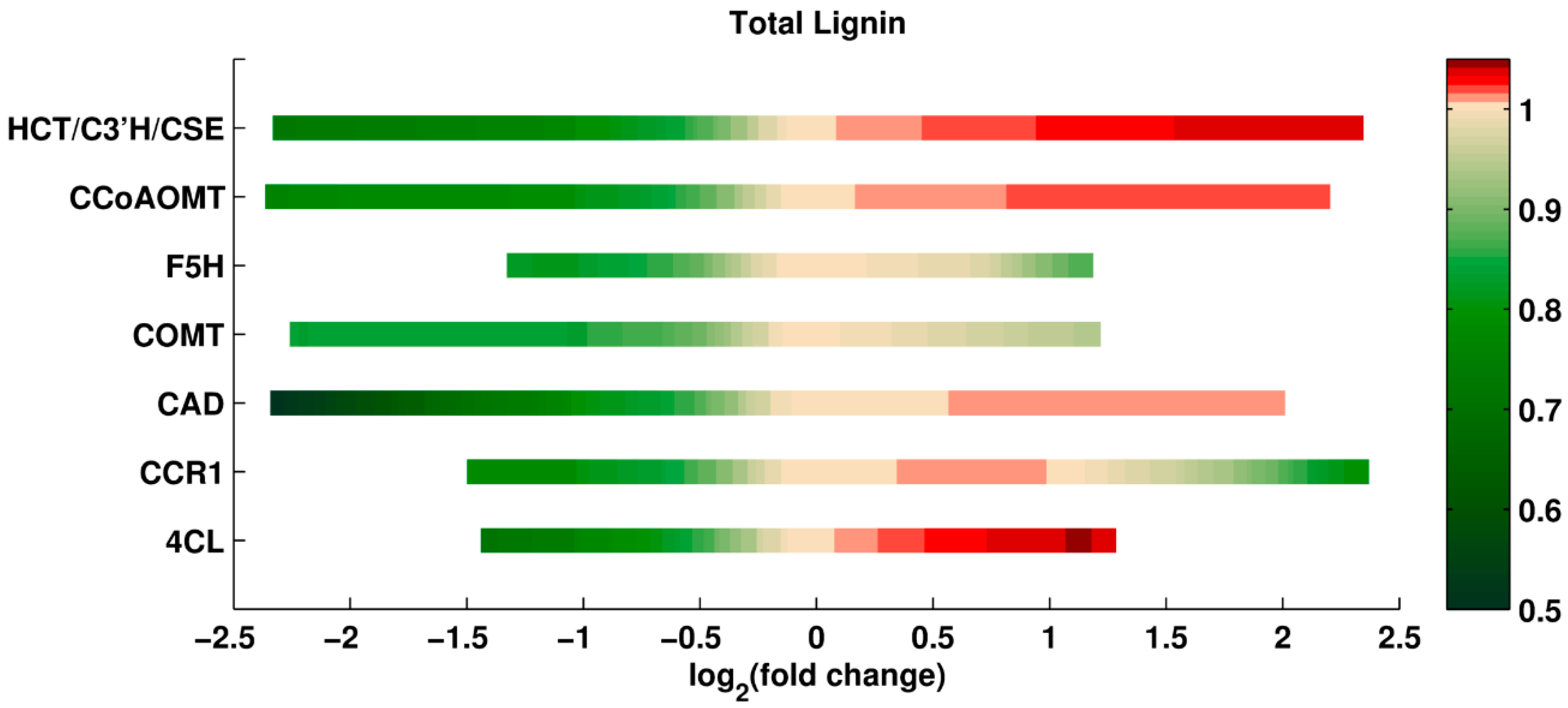
Single Perturbations. In the first set of computational experiments, one enzyme at a time was perturbed up to ±5-fold relative to its wild type activity. Since every scenario is simulated for the entire ensemble of models; the analysis yields many results for each scenario. Using all these results collectively, the median of total lignin content, and the median of the S/G ratio in the perturbed systems are recorded. The medians are normalized with respect to the wild type value, so that value 1 represents the wild type (see Methods).
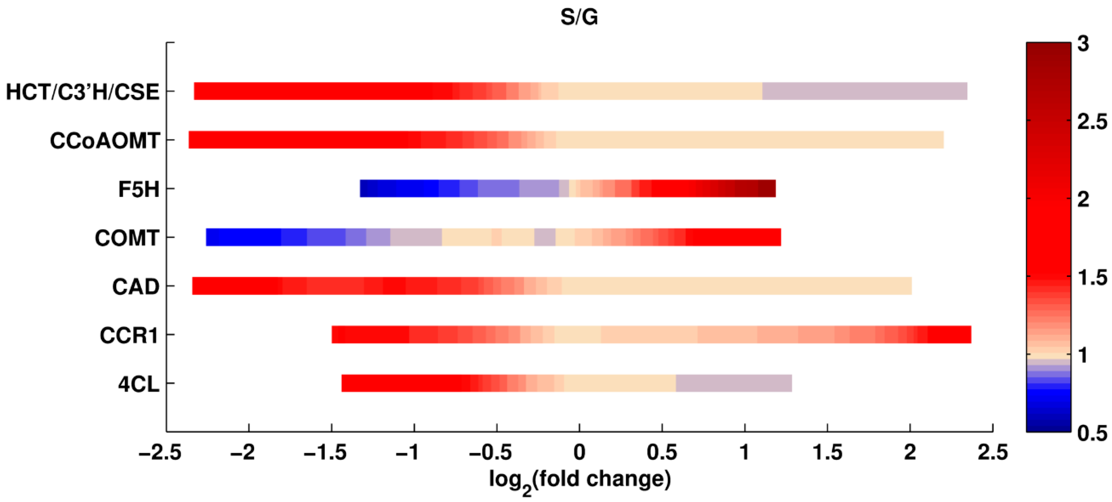
The results of this analysis are shown in Figure 2 and Figure 3. The X-axis shows the log2-fold change in the amount of a given enzyme, and the Y-axis indicates the specifically perturbed enzyme. The grouping of HCT, C3’H, and CSE represents the flux from p-coumaroyl-CoA to caffeic acid, as the corresponding reactions have been merged into one in our model. The color code represents the relative change in total lignin or S/G ratio, for which white depicts no change from the wild type phenotype. The green spectrum (in the panel for total lignin) and the blue spectrum (in the panel for the S/G ratio) represent reductions, while the red spectrum (in both panels) represents an increase relative to wild type. The color bar indicates the intensity of fold change in the enzymes. The greatest lignin reduction achieved is close to 50%, which is the predicted result of an 80% CAD knockdown, with 20% activity remaining. The most significant reduction and increase in S/G ratio is predicted for perturbations in F5H. Thus, the different criteria for total lignin and lignin composition point to different knockdowns.
Double Perturbations. It seems reasonable to surmise that simultaneous changes in two enzymes might be more effective in altering total lignin and/or the S/G ratio. Thus, we analyzed simultaneous perturbations in pairs of enzymes. The perturbations were again restricted to magnitudes of ±5-fold relative to the corresponding wild type activities. Again, every scenario was simulated with the ensemble of models, and the medians of total lignin content and of the S/G ratios were computed and normalized with respect to the wild type values. The results are shown in Figure 4 and Figure 5. The X- and Y-axes represent the log2-fold changes in the perturbed enzyme activities.
It is evident from the results that some perturbations are more effective in altering lignin content and S/G ratio, whereas the system response is more robust to others. It is also clear that many solutions reveal compromises between alterations in total lignin and the S/G ratio. If the S/G ratio is to be altered, F5H seems again to be the key enzyme, and pairs like F5H/4CL, F5H/CCR, F5H/CAD, and F5H/COMT are predicted to be most successful. At the same time, if the goal is solely to reduce lignin, irrespective of the S/G ratio, other solutions exist, including the pairs of CAD/4CL, CAD/CCR, and CAD/F5H.
Single Perturbations in a PvMYB4 Overexpression Strain. A recent study [41,149] analyzed the consequences of overexpressing the inhibitor, PvMYB4, of a transcription factor in switchgrass. The main result was an altered expression profile of many of the enzymes involved in lignin biosynthesis. Consequently, the lignin content was reduced to 40–70%, while the S/G ratio remained the same as for wild type. So far, the PvMYB4 strain has been the most effective transgenic line in reducing recalcitrance in switchgrass. To build upon this success, we combined this scenario with additional single enzyme perturbations, and investigated whether it could be possible to improve the results from the PvMYB4 transgenic strain further. As before, each enzyme was perturbed up to ±5-fold relative to the wild type level. Simulation results are shown in Figure 6 and Figure 7. The color code is the same as for previous figures. The black square in each row represents the enzyme activity in the reference PvMYB4 perturbation. An interesting observation is that the lignin content is predicted to decrease even more than in the reference PvMYB4 experiment if CCR1 is overexpressed in this background. Additional simulations show that lignin content could be reduced further if CCoAOMT, CAD, or 4CL are reduced to even lower levels relative to the PvMYB4 background.
2.4.2. System Optimization through Global Perturbations
So far, all perturbation profiles were determined by Monte Carlo sampling, where the goal was to find a desired combination of lignin content and composition. Now, we pursue a somewhat similar goal, except that it represents a different intent. Namely, a desired target combination of lignin content and S/G ratio is chosen a priori as the criterion for an optimization, where the goal is to determine those admissible combinatorial perturbation profiles that satisfy the criteria in an optimal manner. The main difference between this approach, and the results in Figure 2, Figure 3, Figure 4 and Figure 5, is that the earlier approach tries to keep the number of enzymes to be manipulated as low as possible. Hence, the reduction in lignin content and composition is certainly not necessarily optimized. Furthermore, the changes were restricted by physiological limits, because dramatic changes in enzyme activities may lead to instability of the system, which might translate into the accumulation of toxic intermediate metabolites, or the emergence of undesired phenotypes. Therefore, the level of perturbations should be accordingly limited for at least some enzymes of the pathway.
A different approach toward identifying desirable strains is the optimization of all enzymes within physiological bounds. Although the optimized combinations might not be experimentally implementable at present, they do indicate what changes are theoretically achievable, and in which specific directions novel alterations should be pursued. Thus, this part of the project aims to compute ensembles of optimized enzyme activity patterns within physiological constraints.
As it is not clear which combination of lignin content and composition (S/G ratio) is considered optimal for a particular purpose, all enzymes in the model were simultaneously perturbed randomly up to ±5-fold, using Monte Carlo simulations. Admissible system responses were defined as stable scenarios that reached a steady state and led to an accumulation of metabolites, of at most, 6 times their normal levels, or fell at most, to 5% of the normal level. The admissible solutions were recorded and categorized based on lignin content and S/G ratio.
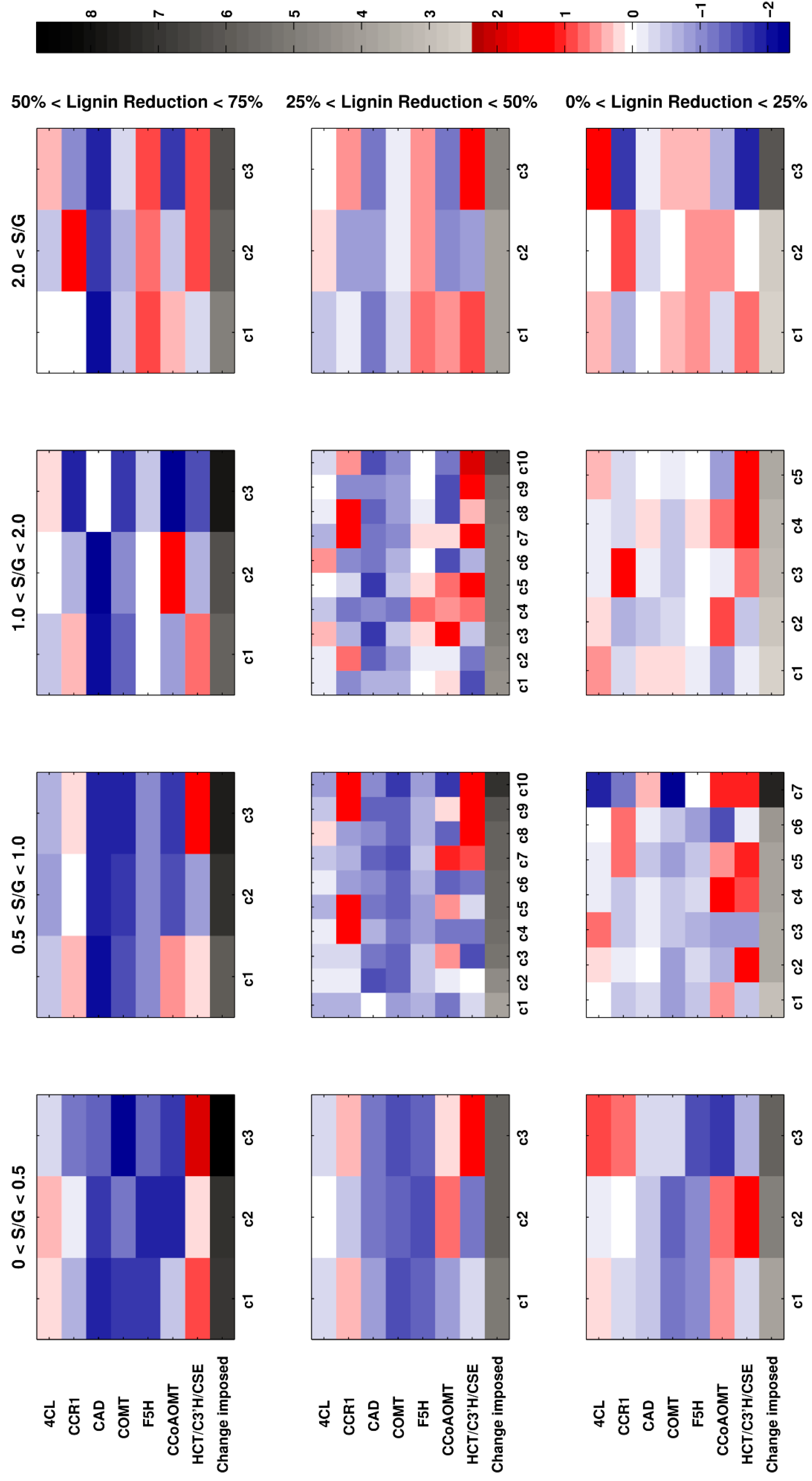
The results are shown in Figure 8. The three rows of subpanels represent the degree of reduction in lignin, categorized in three intervals, and the four columns of subpanels represent intervals for changes in the S/G ratio. Thus, the top row indicates the strongest reduction in lignin, and the left-most subpanel exhibits the lowest S/G ratios. Due to the randomized nature of the Monte Carlo method, we obtain many perturbation profiles that satisfy the constraints of each subpanel. All such profiles are grouped into 3 to 10 clusters, denoted by ci. The default number of clusters is three, and each cluster contains, at most, 100 profiles. Some subpanels include more clusters, which is an indication of the abundance of admissible profiles for that range of constraints. The median of each set of profiles is computed for each cluster, and the clusters are then sorted based on the total fold change in all enzymes collectively, shown as the bottom row in each subpanel. The darker a box in the bottom row is, the more distant the strain is from wild type switchgrass. This total fold change is a measure of how distant or close a mutant strain is to the wild type. This strategy accounts for the observation that profiles closer to wild type are probably to be favored metabolically, and is in line with the concept of the minimization of metabolic adjustment [45].
Since the S/G ratio in wild type switchgrass is about 1, the central subpanels are closer to the wild type. If an experimentalist is interested in a strain with the strongest possible reduction in lignin, and the highest possible increase in the S/G ratio, the subpanel in the top right corner exhibits perturbation profiles that are predicted to achieve these criteria. Among these, cluster c1 is the closer to wild type than c2 and c3 in the same subpanel. If the c1 column is the chosen profile, the enzyme perturbation scenario is indicated by the color code. White represents the wild type, the blue spectrum represents reduced expression of the enzyme, and the red spectrum shows overexpression. The intensity of the color represents the degree of perturbation needed. The log2-fold change is indicated in the color bar.
As a specific example, suppose that a high increase in S/G ratio and a moderate decrease in total lignin is desired, which leads us to the top right subpanel. If a medium total change in enzyme profile is allowed, we choose column c2 as the perturbation scenario. Then, CCR1 must be overexpressed 2.8-fold, F5H must be overexpressed to 1.6-fold, the flux from the group of HCT/C3’H/CSE must be increased 1.9-fold, while 4CL, COMT, and CCoAOMT must be knocked down, as indicated in the blue range of the color scale.
Although the lignin profile in some pathway enzyme knockdowns has been measured before in vivo [40,42,148,149,150], our results cover seven pathway enzyme knockdowns in single, double, and combinatorial perturbations. The possibly strong ±5-fold perturbations presumably cover the realistic range of behaviors of the lignin biosynthetic pathway in response to gene knockdowns. Determining the total lignin and S/G ratio, simultaneously, provides a powerful tool for lignin researchers to choose the desired knockdown scenario based on the lignin characteristics of choice.
Figure 2, Figure 3, Figure 4, Figure 5, Figure 6, Figure 7 and Figure 8 make it clear that the response of the system is nonlinear in some perturbation scenarios. For instance, in single enzyme perturbations (Figure 2), F5H, COMT, and CCR1 exhibit non-monotonic changes in total lignin, which means that reducing the enzyme concentration is not the only way to reduce lignin content, but that targeted overexpression may lead to the same result. In the specific case of CCR, an increase in total lignin with small degrees of enzyme overexpression, followed by a decrease in total lignin at higher levels of enzyme overexpression, is a good example of the occasional counterintuitive behavior of the pathway. The same pattern is even clearer in double knockdowns, such as the pairs of 4CL–CCR, 4CL–F5H, CCR–CAD, CCR–CCoAOMT, and COMT–CCoAOMT (Figure 3). Another interesting result is that choosing a specific perturbation scenario can retain the same amount of total lignin, while leaving room to adjust the desired S/G ratio, as it is the case for the pair 4CL–F5H: there is no substantial difference in total lignin in the left half of the figure, but there is a drastic change in S/G ratio based on the fold change in F5H. The same applies to other pairs including F5H, and also, for the combination of COMT–CCoAOMT.
The computational model turned out to be helpful for an investigation of the transgenic strain of overexpressed PvMYB4 (Figure 5). It is interesting to note that, similar to single enzyme perturbations, combinations of the profile of pathway enzymes in PvMYB4 line with overexpressed CCR can further improve the reduction in total lignin. Again, the S/G ratio is easy to manipulate, while keeping the total lignin almost unchanged; see for instance, combinations of the profile with F5H or COMT.
An added benefit of the developed library is that our results could be complemented with a record of the ethanol yield in the transgenic plants containing different total lignin contents and different S/G ratios. This record could provide the desired lignin content and S/G ratio, and with this target, one could use our results in Figure 2, Figure 3, Figure 4, Figure 5, Figure 6, Figure 7 and Figure 8 to choose the perturbation scenario needed to achieve the target characteristics in the transgenic plant. In other words, this combination of computational results and literature information could be of value and assistance for the targeted design of transgenic plants.
While, from a technical point of view, growing transgenic plants with more than two knocked down enzymes does not seem to be practical at present, fast and inexpensive computational modeling is not really limited. Thus, it offers the opportunity to investigate more complex perturbation scenarios that could shed light onto virtually optimized transgenics. For example, one could restrict the number of enzymes to be perturbed, or permit higher levels of perturbation to achieve a more significant change in total lignin or S/G ratio (cf. [151]).
Of course, caution is advised, and it will be necessary to validate the predictions with correspondingly manipulated strains. As an example of possibly wrong predictions, a drastic change in an enzyme concentration is not a problem, theoretically, but physiological restrictions might not allow it. It could also happen that a significant change in one or two enzymes might lead to intolerable changes in fluxes, or an accumulation of toxic intermediates within, or outside, the lignin pathway. By contrast, a combination of small changes at multiple locations of the pathway is experimentally more challenging, but might avoid such issues. Thus, there is range of options for reaching the same result. Among these admissible perturbation scenarios, which give the same combination of lignin content and S/G ratio, one should presumably focus on the optimized scenario that reaches the target but deviates the least from the wild type. This overall deviation is reminiscent of the philosophy of the method of minimization of metabolic adjustment (MOMA) [45,85], which we discussed before. It may be assessed with a metric, like the Euclidian distance between the enzyme profiles in the virtual transgenic and the wild type. As one might expect, our results show that the more the lignin content is to be reduced, the further the optimized enzyme perturbation profile deviates from the wild type. Interestingly, the S/G ratio is not particularly sensitive to the distance from the wild type, and for the same lignin content, the optimized enzyme perturbation profiles for different S/G ratios are quite close to each other. In other words, it seems that altering the S/G ratio does not introduce plants with severely altered characteristics.
3. Methods
As described elsewhere [47], the lignin pathway system is modeled by a system of stoichiometric differential equations of the form
Here, each is a metabolite, represent fluxes, and are stoichiometric matrix elements. If flux enters the pool of metabolite , then is 1. If flux leaves the pool of metabolite , is −1, and if the flux has no direct association with metabolite , is zero. If all equations equal zero, the pathway operates at a steady state, where the concentrations do not change.
Each flux in Equation (1) is formulated as a general mass action (GMA) equation within the modeling framework of biochemical systems theory [114,115,116,117,152],
where n is the number of metabolites, and m is the number of enzymes in the system. Furthermore, is the rate constant, for is a metabolite, and for is an enzyme. The metabolites are the dependent variables of the system, whereas the enzymes are considered independent variables that do not change during a computational experiment. The parameters and are called kinetic orders. They determine whether a metabolite or enzyme is involved in a flux or not, and if so, in what manner and how strong. For an enzyme, it is customary to set the value of the kinetic order to 0 or 1, which implies that a particular enzyme is not at all involved in the process, or that the flux is linearly dependent on the activity of enzyme . can take a positive or negative value. If , the metabolite is either a substrate or an activator of the flux , and if , is an inhibitor. Here we assume to range between −1 and 1, which is typical (cf. Ch. 5 of [152]). In the case here, the values of the rate constants and kinetic orders are known from the parameterized model in the previous work [47].
Due to lacking information, the steady-state concentrations of the metabolites and the enzyme activities of the pathway are not known. Hence, normalized concentrations relative to wild type concentrations are used.
3.1. A Library of Virtual Mutant Strains
As a consequence of the normalization of the variables, the values for the enzymes are equal to 1 when a wild type strain is modeled. If a knockdown strain is modeled, the corresponding enzyme will have a value less than 1, and if a strain with an upregulated enzyme is modeled, the corresponding enzyme value will be greater than 1. Once a perturbation by down- or upregulation of an enzyme has been introduced, the system rearranges itself, and typically achieves a new steady state. At this state, at least some of the fluxes and metabolites typically assume new values. Thus, the affected flux becomes
To generate a library of virtual mutants, enzyme concentrations, (), are perturbed up to ±5-fold. If the number of enzymes to be perturbed is , using an extensive Monte Carlo simulation, a hypercube in ℝ is randomly sampled, and the generated set of arrays of random values is fed into the system. Since and are already known, the differential equations can be immediately simulated for single or double alterations, or for the PvMYB4 overexpression strain combined with an additional perturbation.
3.2. Admissible Results
Each scenario corresponds to an array of perturbed enzymes. The total lignin content and S/G ratio for the scenario are recorded, if the perturbed system satisfies the following criteria:
- The system is stable at the steady state, and reaches this state after a perturbation.
- The steady-state values of the metabolites do not exceed a value of 6 times the wild type concentration.
- The steady-state values of the metabolites do not fall below 5% of the wild type value.
Since an ensemble of models is used to simulate each scenario, multiple lignin profiles exist for each perturbation scenario. For visualization purposes, the median of the total lignin and the corresponding S/G ratio of the ensemble for each scenario is plotted against the perturbed enzyme(s).
3.3. Global Perturbations and Optimized Virtual Mutant Strains
All seven enzymes are perturbed simultaneously within a range of up to ±5-fold about the wild type value. Perturbation scenarios that satisfy the criteria described in the previous section are recorded. The recorded results are arranged in a matrix based on the total lignin content and S/G ratio. The total lignin range is subdivided into three intervals, namely for 25–50%, 50–75%, and 75–100% reduction in total lignin relative to the wild type, while the S/G ratio is subdivided into four intervals, namely 0–0.5, 0.5–1, 1–2, and >2. These intervals group the results into 12 sets with different total lignin and S/G ratio characteristics.
Each square in the results matrix contains a set with numerous scenarios satisfying specific interval criteria for total lignin and S/G ratio. To facilitate the interpreting of the results, the scenarios are clustered, and the clusters are sorted based on the distance from the wild type, which reflects the overall change imposed upon the system (Figure 8). This distance is defined as the Euclidian distance between the vector of perturbed enzymes and the vector of the corresponding wild type value. The smaller the distance is, the closer is the virtual mutant is to the wild type (Figure 9).
4. Discussion and Conclusions
The article consists of two parts. In the first, we described generic issues of crop modeling, and illustrated them with prominent methods and applications from the literature. Metabolic modeling in plants does not have as rich a history as in animal cells or bacteria, and many of the computational models developed so far have not been specifically tuned for the distinct physiology of plants. We addressed this issue by elaborating strategies on the basis of the most common mathematical techniques in metabolic modeling, focusing on plant applications, and discussing possible discrepancies between standard applications and the specific attributes of plants.
The hope behind this strategy of representing the field was that experimentalists and modelers may find common ground in this discussion. As plant and crop modeling matures, it seems that the current methods may have to be customized toward the genuine features of plants. This customization will have to be the outcome of an extensive, ongoing dialogue between the experimental and computational communities. Such a dialogue is not always easy, as the different communities use different languages and observe nature from different viewpoints. However, the reward of such a collaboration will be the emergence of new integrative approaches that are able to answer pressing questions of the field and guide future experimentation.
As a pertinent side issue, we discussed the reliability of mechanistic modeling using in vitro data, and the fact that researchers must take caution when drawing conclusions from such models, unless extensive validation against in vivo data supports the model performance. Computational models have been instrumental in demonstrating that even for the best known pathways, where allegedly every element of the system is known, in vitro measurements might not be representative enough to simulate the typically complex in vivo environment [103].
An intriguing aspect of computational modeling is the feature of emergence. One type of the emergence of unexpected behavior occurs when a system or organism is exposed to a new environment, in which case, a model may or may not be able to explain the observations. However, the success of computational models in predicting the emergence of some feature, although it had not been foreseen by experimental data, may sometimes be traced back to the nonlinear nature of biological systems, and the model may even offer explanations. It is clear that plant cells, due to their complexity, are susceptible to such issues.
Many mathematical techniques were reviewed in this study, and numerous other techniques exist that have not yet been applied specifically to plant metabolism. The choice of the best suited technique points to the overriding questions of any modeling effort, namely: what are the phenomena that the model is supposed to explain, and which approaches are most efficacious for analyzing the available data? The dichotomies of steady-state or dynamic, deterministic versus stochastic, mechanistic or non-mechanistic models are important choices that a modeler needs to make at the beginning of every analysis, and that ultimately define the quality of a model.
We demonstrated the potential of a model to guide future research in the second part of this article, which was dedicated to a detailed case study. Specifically, we used an earlier model to illustrate how model predictions may provide guideposts for future genomic manipulations. As we demonstrated, the computational model of the lignin biosynthetic pathway captured the complexity of the biological systems and led to insights beyond intuition. It also provided a powerful tool for simulating mutant plants with modified lignin characteristics, and prescribed single, double, combinatorial and global pathway enzyme knockdowns that were predicted to yield plant designs with specifically altered lignin content and composition. The model itself had been validated against a PvMYB4 strain before generating the libraries, but it is clear that further validation against other transgenics will improve the reliability of the presented results, and may improve the model itself.
Acknowledgments
This work was supported by DOE-BESC grant DE-AC05-00OR22725 (PI: Paul Gilna). BESC, the BioEnergy Science Center, is a U.S. Department of Energy Bioenergy Research Center supported by the Office of Biological and Environmental Research in the DOE Office of Science.
Author Contributions
M.F. designed the model as well as the computational experiments. E.O.V. supervised the project and contributed to all computational aspects. Both authors collaborated on the writing of the article.
Conflicts of Interest
The authors declare no conflicts of interest.
Abbreviations
| PAL | L-phenylalanine ammonia-lyase |
| C4H | cinnamate 4-hydroxylase |
| 4CL | 4-coumarate:CoA ligase |
| CCR1 | cinnamoyl CoA reductase 1 |
| CAD | cinnamyl alcohol dehydrogenase |
| HCT | hydroxycinnamoyl-CoA:shikimate hydroxycinnamoyl transferase |
| C3′H | p-coumaroyl shikimate 3′-hydroxylase |
| CSE | caffeoyl shikimate esterase |
| COMT | caffeic acid O-methyltransferase |
| CCoAOMT | caffeoyl CoA O-methyltransferase |
| F5H | ferulate 5-hydroxylase |
| ER | endoplasmic reticulum |
| BST | biochemical systems theory |
| GMA | generalized mass action |
| FBA | flux balance analysis |
References
- Doebley, J. Teosinte As a GraHin Crop. Available online: http://teosinte.wisc.edu/grain_Crop.html (accessed on 5 August 2017).
- List of Sequenced Plant Genomes. Available online: http://en.wikipedia.org/wiki/List_of_sequenced_plant_genomes#Gymnosperm (accessed on 5 August 2017).
- The Human Genome Project Completion. Available online: http://www.genome.gov/11006943/human-genome-project-completion-frequently-asked-questions/ (accessed on 5 August 2017).
- Williams, T.C.R.; Miguet, L.; Masakapalli, S.K.; Kruger, N.J.; Sweetlove, L.J.; Ratcliffe, R.G. Metabolic network fluxes in heterotrophic arabidopsis cells: Stability of the flux distribution under different oxygenation conditions. Plant Physiol. 2008, 148, 704–718. [Google Scholar] [CrossRef] [PubMed]
- Yuan, J.S.; Galbraith, D.W.; Dai, S.Y.; Griffin, P.; Stewart, C.N. Plant systems biology comes of age. Trends Plant Sci. 2008, 13, 165–171. [Google Scholar] [CrossRef] [PubMed]
- Human Metabolome Database. Available online: http://www.hmdb.ca/statistics (accessed on 5 August 2017).
- Bionumbers. Available online: http://bionumbers.hms.harvard.edu/bionumber.aspx?id=105634&ver=4 (accessed on 5 August 2017).
- Dixon, R.A.; Strack, D. Phytochemistry meets genome analysis, and beyond. Phytochemistry 2003, 62, 815–816. [Google Scholar] [CrossRef]
- Saito, K.; Matsuda, F. Metabolomics for functional genomics, systems biology, and biotechnology. Annu. Rev. Plant Biol. 2010, 61, 463–489. [Google Scholar] [CrossRef] [PubMed]
- Cao, H.X.; Wang, W.; Le, H.T.T.; Vu, G.T.H. The power of CRISPR-Cas9-induced genome editing to speed up plant breeding. Int. J. Genom. 2016, 2016, 10. [Google Scholar] [CrossRef] [PubMed]
- Shan, Q.; Wang, Y.; Li, J.; Zhang, Y.; Chen, K.; Liang, Z.; Zhang, K.; Liu, J.; Xi, J.J.; Qiu, J.-L.; et al. Targeted genome modification of crop plants using a CRISPR-Cas system. Nat. Biotech. 2013, 31, 686–688. [Google Scholar] [CrossRef] [PubMed]
- Nekrasov, V.; Staskawicz, B.; Weigel, D.; Jones, J.D.G.; Kamoun, S. Targeted mutagenesis in the model plant nicotiana benthamiana using Cas9 rna-guided endonuclease. Nat. Biotech. 2013, 31, 691–693. [Google Scholar] [CrossRef] [PubMed]
- Li, J.F.; Norville, J.E.; Aach, J.; McCormack, M.; Zhang, D.; Bush, J.; Church, G.M.; Sheen, J. Multiplex and homologous recombination-mediated genome editing in Arabidopsis and Nicotiana benthamiana using guide rna and Cas9. Nat. Biotechnol. 2013, 31, 688–691. [Google Scholar] [CrossRef] [PubMed]
- Cai, Y.; Chen, L.; Liu, X.; Guo, C.; Sun, S.; Wu, C.; Jiang, B.; Han, T.; Hou, W. CRISPR/Cas9-mediated targeted mutagenesis of gmft2a delays flowering time in soya bean. Plant Biotechnol. J. 2017. [Google Scholar] [CrossRef] [PubMed]
- Tian, S.; Jiang, L.; Gao, Q.; Zhang, J.; Zong, M.; Zhang, H.; Ren, Y.; Guo, S.; Gong, G.; Liu, F.; et al. Efficient CRISPR-Cas9-based gene knockout in watermelon. Plant Cell Rep. 2017, 36, 399–406. [Google Scholar] [CrossRef] [PubMed]
- Soyk, S.; Muller, N.A.; Park, S.J.; Schmalenbach, I.; Jiang, K.; Hayama, R.; Zhang, L.; Van Eck, J.; Jimenez-Gomez, J.M. Variation in the flowering gene self pruning 5g promotes day-neutrality and early yield in tomato. Nat. Genet. 2017, 49, 162–168. [Google Scholar] [CrossRef] [PubMed]
- Aharoni, A.; Galili, G. Metabolic engineering of the plant primary-secondary metabolism interface. Curr. Opin. Biotechnol. 2011, 22, 239–244. [Google Scholar] [CrossRef] [PubMed]
- Ratcliffe, R.G.; Shachar-Hill, Y. Measuring multiple fluxes through plant metabolic networks. Plant J. Cell Mol. Biol. 2006, 45, 490–511. [Google Scholar] [CrossRef] [PubMed]
- Morgan, J.A.; Rhodes, D. Mathematical modeling of plant metabolic pathways. Metab. Eng. 2002, 4, 80–89. [Google Scholar] [CrossRef] [PubMed]
- Sweetlove, L.J.; Williams, T.C.; Cheung, C.Y.; Ratcliffe, R.G. Modelling metabolic co(2) evolution—A fresh perspective on respiration. Plant Cell Environ. 2013, 36, 1631–1640. [Google Scholar] [CrossRef] [PubMed]
- Nepali, M.R. Polyploidy Breeding. Available online: http://mukeshramjalipb.blogspot.com/2013/03/polyploidy-breeding.html (accessed on 5 August 2017).
- Meru, G. Polyploidy. Available online: http://plantbreeding.coe.uga.edu/index.php?title=5._Polyploidy (accessed on 5 August 2017).
- Lukhtanov, V.A. The blue butterfly Polyommatus (plebicula) atlanticus (lepidoptera, lycaenidae) holds the record of the highest number of chromosomes in the non-polyploid eukaryotic organisms. Comp. Cytogenet. 2015, 9, 683–690. [Google Scholar] [CrossRef] [PubMed]
- Janick, J.; American Society for Horticultural Science. Plant Breeding Reviews; Wiley Blackwell: Hoboken, NJ, USA, 2009; Volume 31. [Google Scholar]
- Yu, J.; Wang, J.; Lin, W.; Li, S.; Li, H.; Zhou, J.; Ni, P.; Dong, W.; Hu, S.; Zeng, C.; et al. The genomes of Oryza sativa: A history of duplications. PLoS Biol. 2005, 3, e38. [Google Scholar] [CrossRef] [PubMed] [Green Version]
- Arnold, A.; Nikoloski, Z. In search for an accurate model of the photosynthetic carbon metabolism. Math. Comput. Simul. 2014, 96, 171–194. [Google Scholar] [CrossRef]
- Szecowka, M.; Heise, R.; Tohge, T.; Nunes-Nesi, A.; Vosloh, D.; Huege, J.; Feil, R.; Lunn, J.; Nikoloski, Z.; Stitt, M.; et al. Metabolic fluxes in an illuminated Arabidopsis rosette. Plant Cell 2013, 25, 694–714. [Google Scholar] [CrossRef] [PubMed]
- Zhu, X.G.; Wang, Y.; Ort, D.R.; Long, S.P. E-photosynthesis: A comprehensive dynamic mechanistic model of c3 photosynthesis: From light capture to sucrose synthesis. Plant Cell Environ. 2013, 36, 1711–1727. [Google Scholar] [CrossRef] [PubMed]
- Arnold, A.; Nikoloski, Z. A quantitative comparison of calvin-benson cycle models. Trends Plant Sci. 2011, 16, 676–683. [Google Scholar] [CrossRef] [PubMed]
- Cheung, C.Y.M.; Poolman, M.G.; Fell, D.A.; Ratcliffe, R.G.; Sweetlove, L.J. A diel flux balance model captures interactions between light and dark metabolism during day-night cycles in c-3 and crassulacean acid metabolism leaves. Plant Physiol. 2014, 165, 917–929. [Google Scholar] [CrossRef] [PubMed]
- Boyle, N.R.; Morgan, J.A. Computation of metabolic fluxes and efficiencies for biological carbon dioxide fixation. Metab. Eng. 2011, 13, 150–158. [Google Scholar] [CrossRef] [PubMed]
- Guo, Y.; Tan, J.L. A kinetic model structure for delayed fluorescence from plants. Biosystems 2009, 95, 98–103. [Google Scholar] [CrossRef] [PubMed]
- Pearcy, R.W.; Gross, L.J.; He, D. An improved dynamic model of photosynthesis for estimation of carbon gain in sunfleck light regimes. Plant Cell Environ. 1997, 20, 411–424. [Google Scholar] [CrossRef]
- Poolman, M.G.; Miguet, L.; Sweetlove, L.J.; Fell, D.A. A genome-scale metabolic model of Arabidopsis and some of its properties. Plant Physiol. 2009, 151, 1570–1581. [Google Scholar] [CrossRef] [PubMed]
- Lakshmanan, M.; Zhang, Z.Y.; Mohanty, B.; Kwon, J.Y.; Choi, H.Y.; Nam, H.J.; Kim, D.I.; Lee, D.Y. Elucidating rice cell metabolism under flooding and drought stresses using flux-based modeling and analysis. Plant Physiol. 2013, 162, 2140–2150. [Google Scholar] [CrossRef] [PubMed]
- Sweetlove, L.J.; Beard, K.F.M.; Nunes-Nesi, A.; Fernie, A.R.; Ratcliffe, R.G. Not just a circle: Flux modes in the plant tca cycle. Trends Plant Sci. 2010, 15, 462–470. [Google Scholar] [CrossRef] [PubMed]
- Baghalian, K.; Hajirezaei, M.R.; Schreiber, F. Plant metabolic modeling: Achieving new insight into metabolism and metabolic engineering. Plant Cell 2014, 26, 3847–3866. [Google Scholar] [CrossRef] [PubMed]
- Rohwer, J.M. Kinetic modelling of plant metabolic pathways. J. Exp. Bot. 2012, 63, 2275–2292. [Google Scholar] [CrossRef] [PubMed]
- Boerjan, W.; Ralph, J.; Baucher, M. Lignin biosynthesis. Annu. Rev. Plant Biol. 2003, 54, 519–546. [Google Scholar] [CrossRef] [PubMed]
- Xu, B.; Escamilla-Treviño, L.L.; Sathitsuksanoh, N.; Shen, Z.; Shen, H.; Zhang, Y.H.; Dixon, R.A.; Zhao, B. Silencing of 4-coumarate: Coenzyme a ligase in switchgrass leads to reduced lignin content and improved fermentable sugar yields for biofuel production. New Phytol. 2011, 192, 611–625. [Google Scholar] [CrossRef] [PubMed]
- Shen, H.; Poovaiah, C.R.; Ziebell, A.; Tschaplinski, T.J.; Pattathil, S.; Gjersing, E.; Engle, N.L.; Katahira, R.; Pu, Y.; Sykes, R.; et al. Enhanced characteristics of genetically modified switchgrass (Panicum virgatum L.) for high biofuel production. Biotechnol. Biofuels 2013, 6, 71. [Google Scholar] [CrossRef] [PubMed]
- Fu, C.X.; Xiao, X.R.; Xi, Y.J.; Ge, Y.X.; Chen, F.; Bouton, J.; Dixon, R.A.; Wang, Z.Y. Downregulation of cinnamyl alcohol dehydrogenase (cad) leads to improved saccharification efficiency in switchgrass. Bioenerg. Res. 2011, 4, 153–164. [Google Scholar] [CrossRef]
- Tschaplinski, T.J.; Standaert, R.F.; Engle, N.L.; Martin, M.Z.; Sangha, A.K.; Parks, J.M.; Smith, J.C.; Samuel, R.; Jiang, N.; Pu, Y.; et al. Down-regulation of the caffeic acid o-methyltransferase gene in switchgrass reveals a novel monolignol analog. Biotechnol. Biofuels 2012, 5, 71. [Google Scholar] [CrossRef] [PubMed]
- Lee, Y.; Voit, E.O. Mathematical modeling of monolignol biosynthesis in populus xylem. Math. Biosci. 2010, 228, 78–89. [Google Scholar] [CrossRef] [PubMed]
- Lee, Y.; Chen, F.; Gallego-Giraldo, L.; Dixon, R.A.; Voit, E.O. Integrative analysis of transgenic alfalfa (Medicago sativa L.) suggests new metabolic control mechanisms for monolignol biosynthesis. PLoS Comput. Biol. 2011, 7, e1002047. [Google Scholar] [CrossRef] [PubMed]
- Wang, J.P.; Naik, P.P.; Chen, H.C.; Shi, R.; Lin, C.Y.; Liu, J.; Shuford, C.M.; Li, Q.; Sun, Y.H.; Tunlaya-Anukit, S.; et al. Complete proteomic-based enzyme reaction and inhibition kinetics reveal how monolignol biosynthetic enzyme families affect metabolic flux and lignin in populus trichocarpa. Plant Cell 2014, 26, 894–914. [Google Scholar] [CrossRef] [PubMed]
- Faraji, M.; Fonseca, L.L.; Escamilla-Treviño, L.; Dixon, R.A.; Voit, E.O. Computational inference of the structure and regulation of the lignin pathway in panicum virgatum. Biotechnol. Biofuels 2015, 8, 151. [Google Scholar] [CrossRef] [PubMed]
- Amthor, J.S. Efficiency of lignin biosynthesis: A quantitative analysis. Ann. Bot. 2003, 91, 673–695. [Google Scholar] [CrossRef] [PubMed]
- Saha, R.; Suthers, P.F.; Maranas, C.D. Zea mays irs1563: A comprehensive genome-scale metabolic reconstruction of maize metabolism. PLoS ONE 2011, 6, e21784. [Google Scholar] [CrossRef] [PubMed]
- Faraji, M.; Fonseca, L.L.; Escamilla-Trevino, L.; Barros-Rios, J.; Engle, N.; Yang, Z.K.; Tschaplinski, T.J.; Dixon, R.A.; Voit, E.O. Mathematical models of lignin biosynthesis. Biotechnol. Biofuels 2017. under review. [Google Scholar]
- Marshall-Colon, A.; Long, S.P.; Allen, D.K.; Allen, G.; Beard, D.A.; Benes, B.; von Caemmerer, S.; Christensen, A.J.; Cox, D.J.; Hart, J.C.; et al. Crops in silico: Generating virtual crops using an integrative and multi-scale modeling platform. Front. Plant Sci. 2017, 8. [Google Scholar] [CrossRef] [PubMed]
- Crops in Silico. Available online: http://cropsinsilico.org/uiucncsa/ (accessed on 5 August 2017).
- Bogart, E.; Myers, C.R. Multiscale metabolic modeling of c4 plants: Connecting nonlinear genome-scale models to leaf-scale metabolism in developing maize leaves. PLoS ONE 2016, 11, e0151722. [Google Scholar] [CrossRef] [PubMed]
- WIMOVAC (Windows Intuitive Model of Vegetation Response to Atmospheric and Climate Change). Available online: http://www.life.illinois.edu/plantbio/wimovac/ (accessed on 5 August 2017).
- SOYSIM—Soybean Growth Simulation Model. Available online: http://soysim.unl.edu/ (accessed on 5 August 2017).
- Voit, E.O. Models-of-data and models-of-processes in the post-genomic era. Math. Biosci. 2002, 180, 263–274. [Google Scholar] [CrossRef]
- Wiechert, W. C-13 metabolic flux analysis. Metab. Eng. 2001, 3, 195–206. [Google Scholar] [CrossRef] [PubMed]
- Wiechert, W.; Mollney, M.; Petersen, S.; de Graaf, A.A. A universal framework for c-13 metabolic flux analysis. Metab. Eng. 2001, 3, 265–283. [Google Scholar] [CrossRef] [PubMed]
- Maarleveld, T.R.; Khandelwal, R.A.; Olivier, B.G.; Teusink, B.; Bruggeman, F.J. Basic concepts and principles of stoichiometric modeling of metabolic networks. Biotechnol. J. 2013, 8, 997–1008. [Google Scholar] [CrossRef] [PubMed]
- Libourel, I.G.; Shachar-Hill, Y. Metabolic flux analysis in plants: From intelligent design to rational engineering. Ann. Rev. Plant Biol. 2008, 59, 625–650. [Google Scholar] [CrossRef] [PubMed]
- Kruger, N.J.; Ratcliffe, R.G. Insights into plant metabolic networks from steady-state metabolic flux analysis. Biochimie 2009, 91, 697–702. [Google Scholar] [CrossRef] [PubMed]
- Allen, D.K.; Libourel, I.G.; Shachar-Hill, Y. Metabolic flux analysis in plants: Coping with complexity. Plant Cell Environ. 2009, 32, 1241–1257. [Google Scholar] [CrossRef] [PubMed]
- Schwender, J.; Goffman, F.; Ohlrogge, J.B.; Shachar-Hill, Y. Rubisco without the calvin cycle improves the carbon efficiency of developing green seeds. Nature 2004, 432, 779–782. [Google Scholar] [CrossRef] [PubMed]
- Sweetlove, L.J.; Ratcliffe, R.G. Flux-balance modeling of plant metabolism. Front. Plant Sci. 2011, 2. [Google Scholar] [CrossRef] [PubMed]
- Varma, A.; Palsson, B.O. Metabolic flux balancing—Basic concepts, scientific and practical use. Bio-Technology 1994, 12, 994–998. [Google Scholar] [CrossRef]
- Edwards, J.S.; Palsson, B.O. Systems properties of the Haemophilus influenzae Rd metabolic genotype. J. Biol. Chem. 1999, 274, 17410–17416. [Google Scholar] [CrossRef] [PubMed]
- Heinrich, R.; Schuster, S. The Regulation of Cellular Systems; Chapman & Hall: New York, NY, USA, 1996; p. vix. 327p. [Google Scholar]
- Gavalas, G.R. Nonlinear Differential Equations of Chemically Reacting Systems; Springer Verlag: New York, NY, USA, 1968; 106p. [Google Scholar]
- Palsson, B. Systems Biology: Properties of Reconstructed Networks; Cambridge University Press: New York, NY, USA, 2006; p. xii. 322p. [Google Scholar]
- Mahadevan, R.; Schilling, C.H. The effects of alternate optimal solutions in constraint-based genome-scale metabolic models. Metab. Eng. 2003, 5, 264–276. [Google Scholar] [CrossRef] [PubMed]
- Schuster, S.H.S. On elementary flux modes in biochemical reaction systems at steady state. J. Biol. Syst. 1994, 2, 165–182. [Google Scholar] [CrossRef]
- Trinh, C.T.; Wlaschin, A.; Srienc, F. Elementary mode analysis: A useful metabolic pathway analysis tool for characterizing cellular metabolism. Appl. Microbiol. Biotechnol. 2009, 81, 813–826. [Google Scholar] [CrossRef] [PubMed]
- Kruger, N.J.; Masakapalli, S.K.; Ratcliffe, R.G. Strategies for investigating the plant metabolic network with steady-state metabolic flux analysis: Lessons from an Arabidopsis cell culture and other systems. J. Exp. Bot. 2012, 63, 2309–2323. [Google Scholar] [CrossRef] [PubMed]
- Kacser, H.; Burns, J.A. The control of flux. Symp. Soc. Exp. Biol. 1973, 27, 65–104. [Google Scholar] [CrossRef] [PubMed]
- Heinrich, R.; Rapoport, T.A. A linear steady-state treatment of enzymatic chains. Critique of the crossover theorem and a general procedure to identify interaction sites with an effector. Eur. J. Biochem. 1974, 42, 97–105. [Google Scholar] [CrossRef] [PubMed]
- Heinrich, R.; Rapoport, T.A. A linear steady-state treatment of enzymatic chains. General properties, control and effector strength. Eur. J. Biochem. 1974, 42, 89–95. [Google Scholar] [CrossRef] [PubMed]
- Fell, D.A. Metabolic control analysis: A survey of its theoretical and experimental development. Biochem. J. 1992, 286 Pt 2, 313–330. [Google Scholar] [CrossRef] [PubMed]
- Orth, J.D.; Thiele, I.; Palsson, B.O. What is flux balance analysis? Nat. Biotechnol. 2010, 28, 245–248. [Google Scholar] [CrossRef] [PubMed]
- Páez Melo, D.O.; Jay-Pang Moncada, R.; Winck, F.V.; Barrios, A.F.G. In silico analysis for biomass synthesis under different CO2 levels for Chlamydomonas reinhardtii utilizing a flux balance analysis approach. In Advances in Intelligent Systems and Computing; Pietka, E., Ed.; Springer International Publishing: Cham, Switzerland, 2014; Volume 232, pp. 279–285. [Google Scholar]
- Chang, R.L.; Ghamsari, L.; Manichaikul, A.; Hom, E.F.; Balaji, S.; Fu, W.; Shen, Y.; Hao, T.; Palsson, B.O.; Salehi-Ashtiani, K.; et al. Metabolic network reconstruction of Chlamydomonas offers insight into light-driven algal metabolism. Mol. Syst. Biol. 2011, 7, 518. [Google Scholar] [CrossRef] [PubMed]
- Flassig, R.J.; Fachet, M.; Hoffner, K.; Barton, P.I.; Sundmacher, K. Dynamic flux balance modeling to increase the production of high-value compounds in green microalgae. Biotechnol. Biofuels 2016, 9, 165. [Google Scholar] [CrossRef] [PubMed]
- Sengupta, T.; Bhushan, M.; Wangikar, P.P. Metabolic modeling for multi-objective optimization of ethanol production in a Synechocystis mutant. Photosynth. Res. 2013, 118, 155–165. [Google Scholar] [CrossRef] [PubMed]
- Villaverde, A.F.; Bongard, S.; Mauch, K.; Balsa-Canto, E.; Banga, J.R. Metabolic engineering with multi-objective optimization of kinetic models. J. Biotechnol. 2016, 222, 1–8. [Google Scholar] [CrossRef] [PubMed]
- Barros, J.; Serrani-Yarce, J.C.; Chen, F.; Baxter, D.; Venables, B.J.; Dixon, R.A. Role of bifunctional ammonia-lyase in grass cell wall biosynthesis. Nat. Plants 2016, 2, 16050. [Google Scholar] [CrossRef] [PubMed]
- Segre, D.; Vitkup, D.; Church, G.M. Analysis of optimality in natural and perturbed metabolic networks. Proc. Natl. Acad. Sci. USA 2002, 99, 15112–15117. [Google Scholar] [CrossRef] [PubMed]
- Hay, J.; Schwender, J. Metabolic network reconstruction and flux variability analysis of storage synthesis in developing oilseed rape (Brassica napus L.) embryos. Plant J. Cell Mol. Biol. 2011, 67, 526–541. [Google Scholar] [CrossRef] [PubMed]
- Hay, J.; Schwender, J. Computational analysis of storage synthesis in developing Brassica napus L. (oilseed rape) embryos: Flux variability analysis in relation to (1)(3)c metabolic flux analysis. Plant J. Cell Mol. Biol. 2011, 67, 513–525. [Google Scholar] [CrossRef] [PubMed]
- Steuer, R.; Nesi, A.N.; Fernie, A.R.; Gross, T.; Blasius, B.; Selbig, J. From structure to dynamics of metabolic pathways: Application to the plant mitochondrial tca cycle. Bioinformatics 2007, 23, 1378–1385. [Google Scholar] [CrossRef] [PubMed]
- Schuster, S.; Dandekar, T.; Fell, D.A. Detection of elementary flux modes in biochemical networks: A promising tool for pathway analysis and metabolic engineering. Trends Biotechnol. 1999, 17, 53–60. [Google Scholar] [CrossRef]
- Llaneras, F.; Pico, J. Which metabolic pathways generate and characterize the flux space? A comparison among elementary modes, extreme pathways and minimal generators. J. Biomed. Biotechnol. 2010, 2010, 753904. [Google Scholar] [CrossRef] [PubMed]
- Sherry, A.D.; Malloy, C.R. Integration of 13c isotopomer methods and hyperpolarization provides a comprehensive picture of metabolism. In eMagRes; John Wiley & Sons, Ltd.: Chichester, UK, 2007. [Google Scholar]
- Roscher, A.; Kruger, N.J.; Ratcliffe, R.G. Strategies for metabolic flux analysis in plants using isotope labelling. J. Biotechnol. 2000, 77, 81–102. [Google Scholar] [CrossRef]
- Dieuaide-Noubhani, M.; Alonso, A.P. Application of metabolic flux analysis to plants. Methods Mol. Biol. 2014, 1090, 1–17. [Google Scholar] [PubMed]
- Moreno-Sanchez, R.; Saavedra, E.; Rodriguez-Enriquez, S.; Olin-Sandoval, V. Metabolic control analysis: A tool for designing strategies to manipulate metabolic pathways. J. Biomed. Biotechnol. 2008, 2008, 597913. [Google Scholar] [CrossRef] [PubMed]
- Ap Rees, T.; Hill, S.A. Metabolic control analysis of plant metabolism. Plant Cell Environ. 1994, 17, 587–599. [Google Scholar] [CrossRef]
- Giersch, C.; Lämmel, D.; Farquhar, G. Control analysis of photosynthetic CO2 fixation. Photosynth. Res. 1990, 24, 151–165. [Google Scholar] [PubMed]
- Waage, P.; Gulberg, C.M. Studies concerning affinity. J. Chem. Educ. 1986, 63, 1044. [Google Scholar] [CrossRef]
- Farré, G.; Maiam Rivera, S.; Alves, R.; Vilaprinyo, E.; Sorribas, A.; Canela, R.; Naqvi, S.; Sandmann, G.; Capell, T.; Zhu, C.; et al. Targeted transcriptomic and metabolic profiling reveals temporal bottlenecks in the maize carotenoid pathway that may be addressed by multigene engineering. Plant J. 2013, 75, 441–455. [Google Scholar] [CrossRef] [PubMed]
- Bai, C.; Rivera, S.M.; Medina, V.; Alves, R.; Vilaprinyo, E.; Sorribas, A.; Canela, R.; Capell, T.; Sandmann, G.; Christou, P.; et al. An in vitro system for the rapid functional characterization of genes involved in carotenoid biosynthesis and accumulation. Plant J. 2014, 77, 464–475. [Google Scholar] [CrossRef] [PubMed]
- Michaelis, L.; Menten, M.L. Die Kinetik der Invertinwirkung. Biochem. Z. 1913, 49, 333–369. [Google Scholar]
- Henri, V. Lois Générales de L'action des Diastases; Librairie Scientifique A. Hermann: Paris, France, 1903; p. viii. 129p. [Google Scholar]
- Cornish-Bowden, A. One hundred years of Michaelis–Menten kinetics. Perspect. Sci. 2015, 4, 3–9. [Google Scholar] [CrossRef]
- Teusink, B.; Passarge, J.; Reijenga, C.A.; Esgalhado, E.; van der Weijden, C.C.; Schepper, M.; Walsh, M.C.; Bakker, B.M.; van Dam, K.; Westerhoff, H.V.; et al. Can yeast glycolysis be understood in terms of in vitro kinetics of the constituent enzymes? Testing biochemistry. Eur. J. Biochem. 2000, 267, 5313–5329. [Google Scholar] [CrossRef] [PubMed]
- Schulz, A.R. Enzyme Kinetics: From Diastase to Multi-Enzyme Systems; Cambridge University Press: New York, NY, USA, 1994; p. x. 246p. [Google Scholar]
- Hill, A.V. The possible effects of the aggregation of the molecules of haemoglobin on its dissociation curves. J. Physiol. 1910, 40, 4–7. [Google Scholar]
- Nag, A.; Lunacek, M.; Graf, P.A.; Chang, C.H. Kinetic modeling and exploratory numerical simulation of chloroplastic starch degradation. BMC Syst. Biol. 2011, 5, 94. [Google Scholar] [CrossRef] [PubMed]
- Cornish-Bowden, A. Fundamentals of Enzyme Kinetics, 3rd ed.; Portland Press: London, UK, 2004; p. xvi. 422p. [Google Scholar]
- Voit, E.O. The best models of metabolism. Wiley Interdisciplin. Rev. Syst. Biol. Med. 2017. [Google Scholar] [CrossRef] [PubMed]
- Lee, Y.; Escamilla-Trevino, L.; Dixon, R.A.; Voit, E.O. Functional analysis of metabolic channeling and regulation in lignin biosynthesis: A computational approach. PLoS Comput. Biol. 2012, 8, e1002769. [Google Scholar] [CrossRef] [PubMed]
- Steuer, R.; Gross, T.; Selbig, J.; Blasius, B. Structural kinetic modeling of metabolic networks. Proc. Natl. Acad. Sci. USA 2006, 103, 11868–11873. [Google Scholar] [CrossRef] [PubMed]
- Goel, G.; Chou, I.C.; Voit, E.O. System estimation from metabolic time-series data. Bioinformatics 2008, 24, 2505–2511. [Google Scholar] [CrossRef] [PubMed]
- Faraji, M.; Voit, E.O. Nonparametric dynamic modeling. Math. Biosci. 2017, 287, 130–146. [Google Scholar] [CrossRef] [PubMed]
- Faraji, M.; Voit, E.O. Stepwise inference of likely dynamic flux distributions from metabolic time series data. Bioinformatics 2017. [Google Scholar] [CrossRef] [PubMed]
- Savageau, M.A. Biochemical systems analysis. I. Some mathematical properties of the rate law for the component enzymatic reactions. J. Theor. Biol. 1969, 25, 365–369. [Google Scholar] [CrossRef]
- Savageau, M.A. Biochemical systems analysis. Ii. The steady-state solutions for an n-pool system using a power-law approximation. J. Theor. Biol. 1969, 25, 370–379. [Google Scholar] [CrossRef]
- Savageau, M.A. Biochemical Systems Analysis: A Study of Function and Design in Molecular Biology; Addison-Wesley Pub. Co. Advanced Book Program: Reading, Massachusetts, USA, 1976; p. xvii. 379p. [Google Scholar]
- Voit, E.O. Biochemical systems theory: A review. ISRN Biomath. 2013, 2013, 53. [Google Scholar] [CrossRef]
- Voit, E.O. Dynamics of self-thinning plant stands. Ann. Bot. 1988, 62, 67–78. [Google Scholar] [CrossRef]
- Torsella, J.; Bin Razali, A. An analysis of forestry data. In Canonical Nonlinear Modeling: S-System Approach to Understanding Complexity; Voit, E.O., Ed.; Van Nostrand Reinhold: New York, NY, USA, 1991; pp. 181–199. [Google Scholar]
- Torres, N.V. S-system modelling approach to ecosystem: Application to a study of magnesium flow in a tropical forest. Ecol. Model. 1996, 89, 109–120. [Google Scholar] [CrossRef]
- Sands, P.; Voit, E. Flux-based estimation of parameters in s-systems. Ecol. Model. 1996, 93, 75–88. [Google Scholar] [CrossRef]
- Voit, E.O.; Sands, P.J. Modeling forest growth ii. Biomass partitioning in scots pine. Ecol. Model. 1996, 86, 73–89. [Google Scholar] [CrossRef]
- Martin, P.-G. The use of canonical S-system modelling for condensation of complex dynamic models. Ecol. Model. 1997, 103, 43–70. [Google Scholar] [CrossRef]
- Kaitaniemi, P. A canonical model of tree resource allocation after defoliation and bud consumption. Ecol. Model. 2000, 129, 259–272. [Google Scholar] [CrossRef]
- Renton, M.; Kaitaniemi, P.; Hanan, J. Functional–structural plant modelling using a combination of architectural analysis, l-systems and a canonical model of function. Ecol. Model. 2005, 184, 277–298. [Google Scholar] [CrossRef]
- Sorribas, A.; Hernandez-Bermejo, B.; Vilaprinyo, E.; Alves, R. Cooperativity and saturation in biochemical networks: A saturable formalism using Taylor series approximations. Biotechnol. Bioeng. 2007, 97, 1259–1277. [Google Scholar] [CrossRef] [PubMed]
- Wu, L.; Wang, W.; van Winden, W.A.; van Gulik, W.M.; Heijnen, J.J. A new framework for the estimation of control parameters in metabolic pathways using lin-log kinetics. Eur. J. Biochem. 2004, 271, 3348–3359. [Google Scholar] [CrossRef] [PubMed]
- Visser, D.; Heijnen, J.J. Dynamic simulation and metabolic re-design of a branched pathway using linlog kinetics. Metab. Eng. 2003, 5, 164–176. [Google Scholar] [CrossRef]
- Heijnen, J.J. Approximative kinetic formats used in metabolic network modeling. Biotechnol. Bioeng. 2005, 91, 534–545. [Google Scholar] [CrossRef] [PubMed]
- Del Rosario, R.C.H.; Mendoza, E.; Voit, E.O. Challenges in lin-log modelling of glycolysis in Lactococcus lactis. IET Syst. Biol. 2008, 2, 136–149. [Google Scholar] [CrossRef] [PubMed]
- Wang, F.S.; Ko, C.L.; Voit, E.O. Kinetic modeling using S-systems and lin-log approaches. Biochem. Eng. J. 2007, 33, 238–247. [Google Scholar] [CrossRef]
- Chou, I.C.; Voit, E.O. Estimation of dynamic flux profiles from metabolic time series data. BMC Syst. Biol. 2012, 6, 84. [Google Scholar] [CrossRef] [PubMed]
- Dolatshahi, S.; Voit, E.O. Identification of metabolic pathway systems. Front. Genet. 2016, 7, 6. [Google Scholar] [CrossRef] [PubMed]
- Iwata, M.; Shiraishi, F.; Voit, E.O. Coarse but efficient identification of metabolic pathway systems. Int. J. Syst. Biol. 2013, 4, 57. [Google Scholar]
- Voit, E.O.; Goel, G.; Chou, I.C.; Fonseca, L.L. Estimation of metabolic pathway systems from different data sources. Iet. Syst. Biol. 2009, 3, 513–522. [Google Scholar] [CrossRef] [PubMed]
- Hartmann, A.; Schreiber, F. Integrative analysis of metabolic models—From structure to dynamics. Front. Bioeng. Biotechnol. 2015, 2. [Google Scholar] [CrossRef] [PubMed]
- Wu, Q.; Tian, T. Stochastic modeling of biochemical systems with multistep reactions using state-dependent time delay. Sci. Rep. 2016, 6, 31909. [Google Scholar] [CrossRef] [PubMed]
- Yu, Y.; Dong, W.; Altimus, C.; Tang, X.; Griffith, J.; Morello, M.; Dudek, L.; Arnold, J.; Schüttler, H.-B. A genetic network for the clock of Neurospora crassa. Proc. Natl. Acad. Sci. USA 2007, 104, 2809–2814. [Google Scholar] [CrossRef] [PubMed]
- Deng, Z.; Arsenault, S.; Caranica, C.; Griffith, J.; Zhu, T.; Al-Omari, A.; Schuttler, H.B.; Arnold, J.; Mao, L. Synchronizing stochastic circadian oscillators in single cells of Neurospora crassa. Sci. Rep. 2016, 6, 35828. [Google Scholar] [CrossRef] [PubMed]
- Guerriero, M.L.; Akman, O.E.; van Ooijen, G. Stochastic models of cellular circadian rhythms in plants help to understand the impact of noise on robustness and clock structure. Front. Plant Sci. 2014, 5, 564. [Google Scholar] [CrossRef] [PubMed] [Green Version]
- Guerriero, M.L.; Pokhilko, A.; Fernández, A.P.; Halliday, K.J.; Millar, A.J.; Hillston, J. Stochastic properties of the plant circadian clock. J. Royal Soc. Interface 2012, 9, 744–756. [Google Scholar] [CrossRef] [PubMed]
- Akman, O.E.; Ciocchetta, F.; Degasperi, A.; Guerriero, M.L. Modelling biological clocks with bio-pepa: Stochasticity and robustness for the Neurospora crassa circadian network. In Proceedings of the Computational Methods in Systems Biology: 7th International Conference (CMSB 2009), Bologna, Italy, 31 August–1 September 2009; Degano, P., Gorrieri, R., Eds.; Springer: Berlin, Heidelberg, 2009; pp. 52–67. [Google Scholar]
- Gonze, D.; Halloy, J.; Goldbeter, A. Deterministic versus stochastic models for circadian rhythms. J. Biol. Phys. 2002, 28, 637–653. [Google Scholar] [CrossRef] [PubMed]
- Sweetlove, L.J.; Fernie, A.R. The spatial organization of metabolism within the plant cell. Annu. Rev. Plant Biol. 2013, 64, 723–746. [Google Scholar] [CrossRef] [PubMed]
- Grafahrend-Belau, E.; Junker, A.; Eschenroder, A.; Muller, J.; Schreiber, F.; Junker, B.H. Multiscale metabolic modeling: Dynamic flux balance analysis on a whole-plant scale. Plant Physiol. 2013, 163, 637–647. [Google Scholar] [CrossRef] [PubMed]
- Davison, B.H.; Drescher, S.R.; Tuskan, G.A.; Davis, M.F.; Nghiem, N.P. Variation of s/g ratio and lignin content in a populus family influences the release of xylose by dilute acid hydrolysis. Appl. Biochem. Biotechnol. 2006, 129–132, 427–435. [Google Scholar] [CrossRef]
- Van Acker, R.; Vanholme, R.; Storme, V.; Mortimer, J.C.; Dupree, P.; Boerjan, W. Lignin biosynthesis perturbations affect secondary cell wall composition and saccharification yield in Arabidopsis thaliana. Biotechnol. Biofuels 2013, 6, 46. [Google Scholar] [CrossRef] [PubMed] [Green Version]
- Escamilla-Trevino, L.L.; Shen, H.; Uppalapati, S.R.; Ray, T.; Tang, Y.; Hernandez, T.; Yin, Y.; Xu, Y.; Dixon, R.A. Switchgrass (Panicum virgatum) possesses a divergent family of cinnamoyl coa reductases with distinct biochemical properties. New Phytol. 2010, 185, 143–155. [Google Scholar] [CrossRef] [PubMed]
- Shen, H.; He, X.; Poovaiah, C.R.; Wuddineh, W.A.; Ma, J.; Mann, D.G.; Wang, H.; Jackson, L.; Tang, Y.; Stewart, C.N., Jr.; et al. Functional characterization of the switchgrass (Panicum virgatum) r2r3-myb transcription factor pvmyb4 for improvement of lignocellulosic feedstocks. New Phytol. 2012, 193, 121–136. [Google Scholar] [CrossRef] [PubMed]
- Fu, C.; Mielenz, J.R.; Xiao, X.; Ge, Y.; Hamilton, C.Y.; Rodriguez, M., Jr.; Chen, F.; Foston, M.; Ragauskas, A.; Bouton, J.; et al. Genetic manipulation of lignin reduces recalcitrance and improves ethanol production from switchgrass. Proc. Natl. Acad. Sci. USA 2011, 108, 3803–3808. [Google Scholar] [CrossRef] [PubMed]
- Torres, N.V.; Voit, E.O. Pathway Analysis and Optimization in Metabolic Engineering; Cambridge University Press: Cambridge, UK; New York, NY, USA, 2002; p. xiv. 305p. [Google Scholar]
- Voit, E.O. Computational Analysis of Biochemical Systems: A Practical Guide for Biochemists and Molecular Biologists; Cambridge University Press: New York, NY, USA, 2000; p. xii. 531p. [Google Scholar]
Figure 1.
Lignin biosynthesis pathway in switchgrass (Panicum virgatum). The pathway mainly uses phenylalanine as starting compound. The reactions take place in the cytosol, and the monolignol end products are translocated to the plant cell wall, transformed into lignin monomers, and polymerized to form lignin. In switchgrass, the overall lignin composition is ~5% H, 45–50% S, and 45–50% G-lignin.
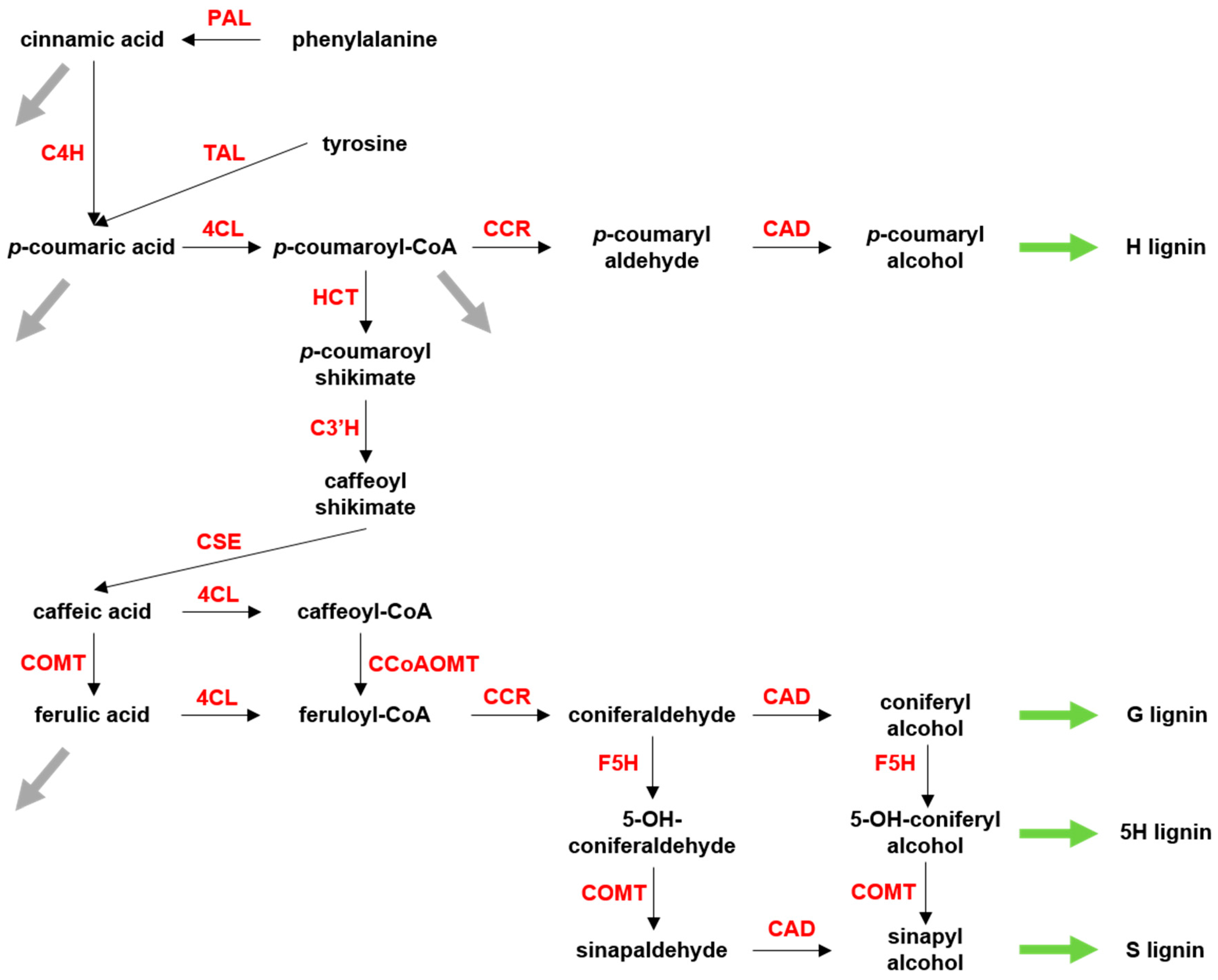
Figure 2.
Total lignin in response to single enzyme perturbations. The total lignin level is color coded, where green represents decreases in total lignin, red represents increases, while white corresponds to the wild type level. CAD seems to be the most effective enzyme in reducing lignin. Note that, surprisingly, the change in lignin content is not always monotonic. Simulations show that lignin can be reduced by knocking down or overexpressing the activities of F5H, COMT and CCR.

Figure 3.
S/G ratios in response to single enzyme perturbations. Blue represents decreases in S/G ratios, red represents increases, while white is the wild type base level. F5H seems to be the most effective enzyme for altering the S/G ratio, both toward increases and decreases. Similar to the total lignin response, changes in S/G ratios are not necessarily monotonic: the S/G ratio increases in both knocked down and overexpressed CCR1.

Figure 4.
Total lignin in double enzyme perturbations. The color code is the same as in Figure 2. Pairs of CAD/4CL, CAD/CCR, and CAD/F5H are predicted as the most effective combinations; in particular, the pair of CAD/F5H shows strong synergism: an increase in F5H, combined with a small reduction in CAD, reduces total lignin dramatically. The nonlinear behavior of the pathway is evident in the dual-overexpression scenarios, especially in pairs, including CCR1, COMT, or F5H.
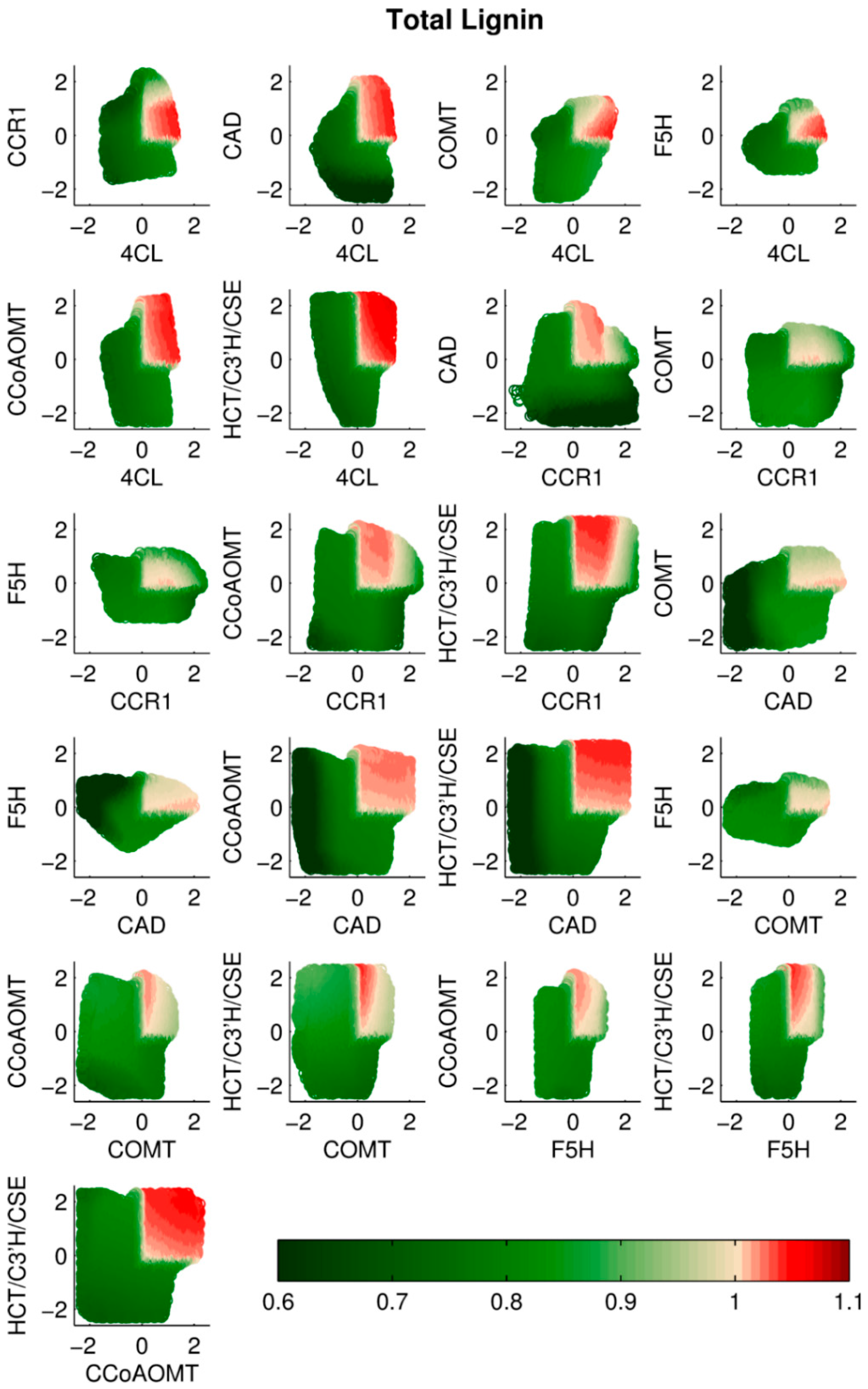
Figure 5.
S/G ratios in response to two simultaneous enzyme perturbations. The color code is the same as in Figure 3. Pairs including F5H and COMT (F5H/4CL, F5H/CCR, F5H/CAD, F5H/COMT, COMT/4CL, COMT/CCR) show the highest changes in S/G ratio. In particular, F5H and COMT work well synergistically, even for moderate perturbations.
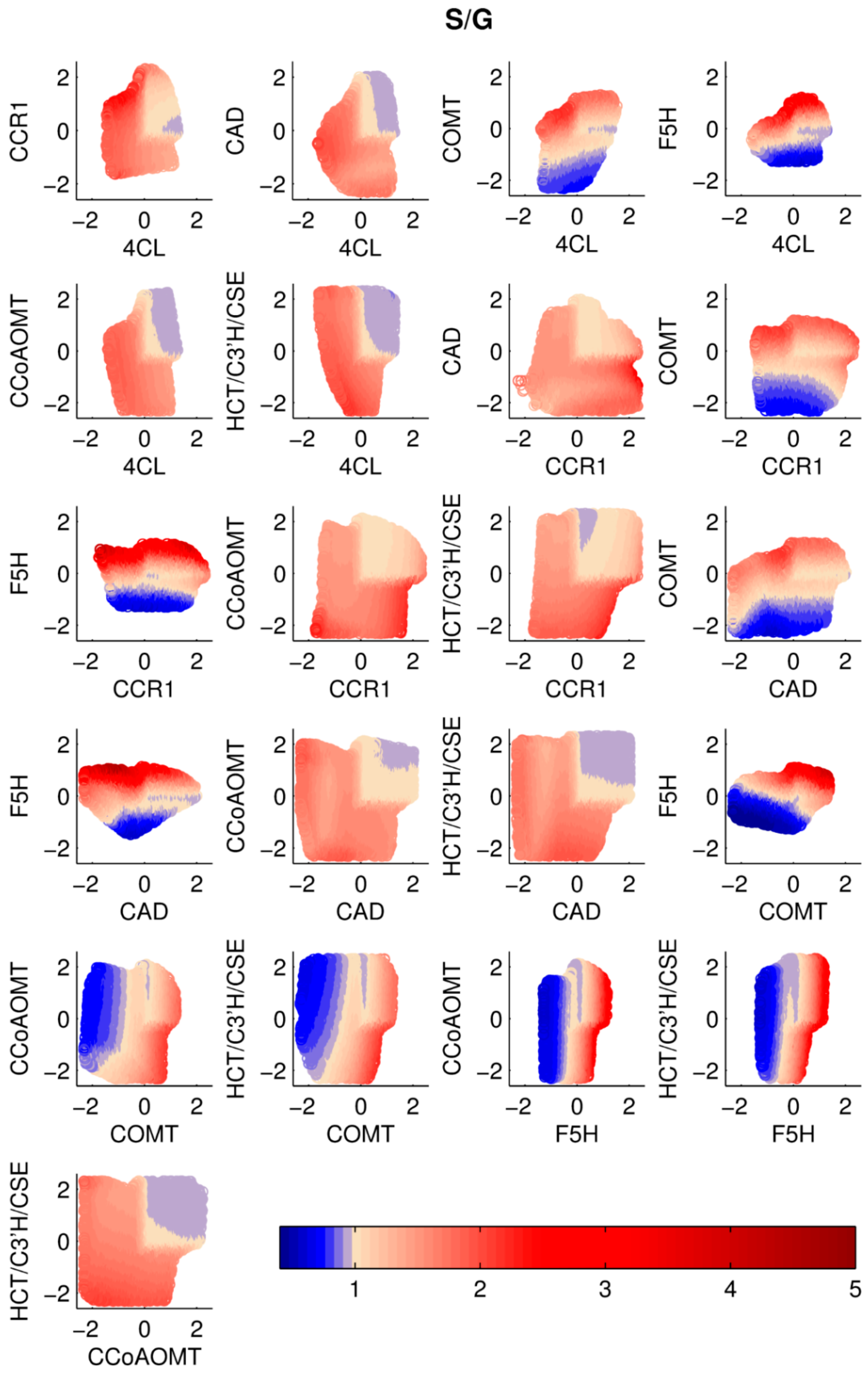
Figure 6.
Total lignin in overexpressed PvMYB4 plus a single enzyme perturbation. The color code is the same as in Figure 2. The black squares represent the original amount of the corresponding enzyme in the PvMYB4 experiment. Additional overexpression of CCR is predicted to improve the total lignin results. Decreasing the level of CAD and CCoAOMT, relative to the reference PvMyb4 experiment, can reduce the total lignin further.
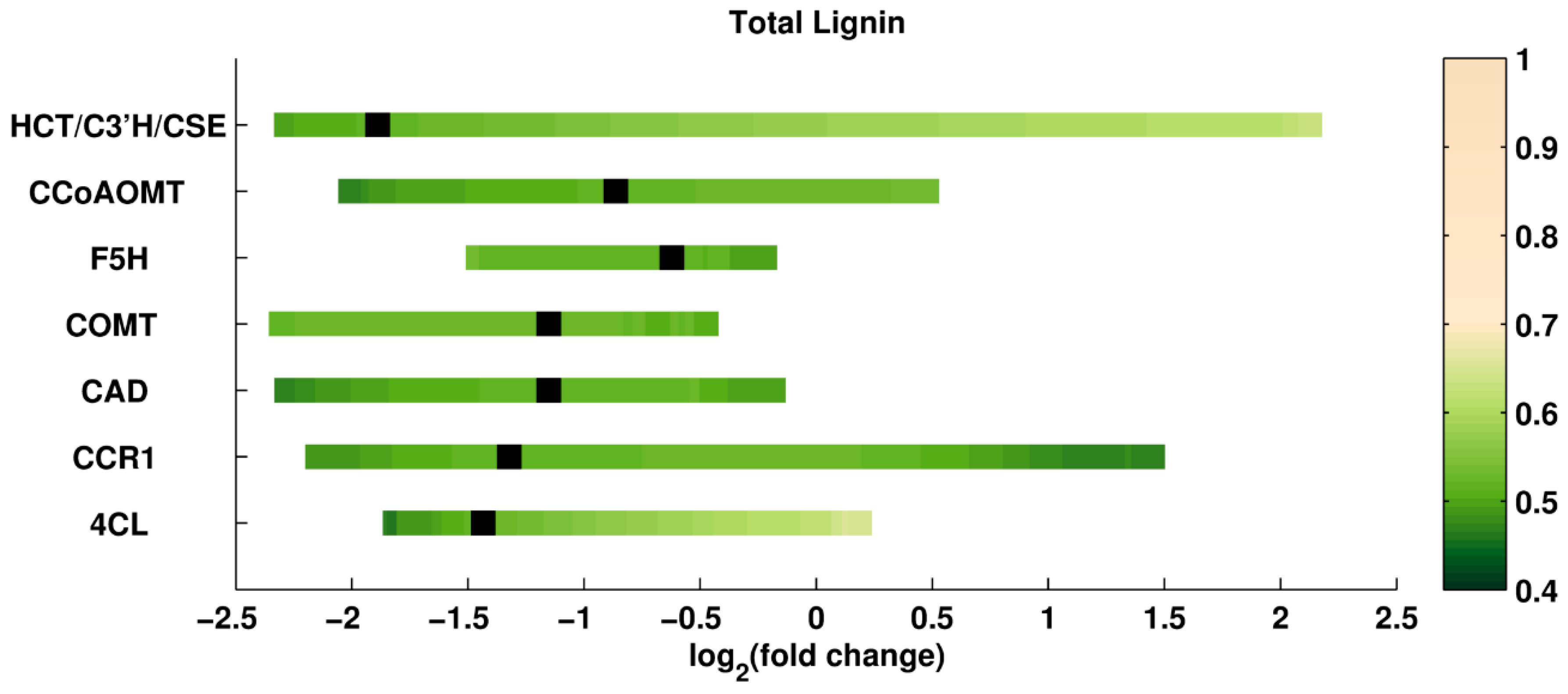
Figure 7.
S/G ratio in overexpressed PvMYB4 plus an additional single enzyme perturbation. The color code is the same as in Figure 3. The black squares represent the reference amount of the corresponding enzyme in the PvMYB4 experiment. The S/G ratio can be significantly changed compared to the background PvMYB4 experiment. A change in F5H can alter the S/G ratio dramatically in a narrow perturbation interval.
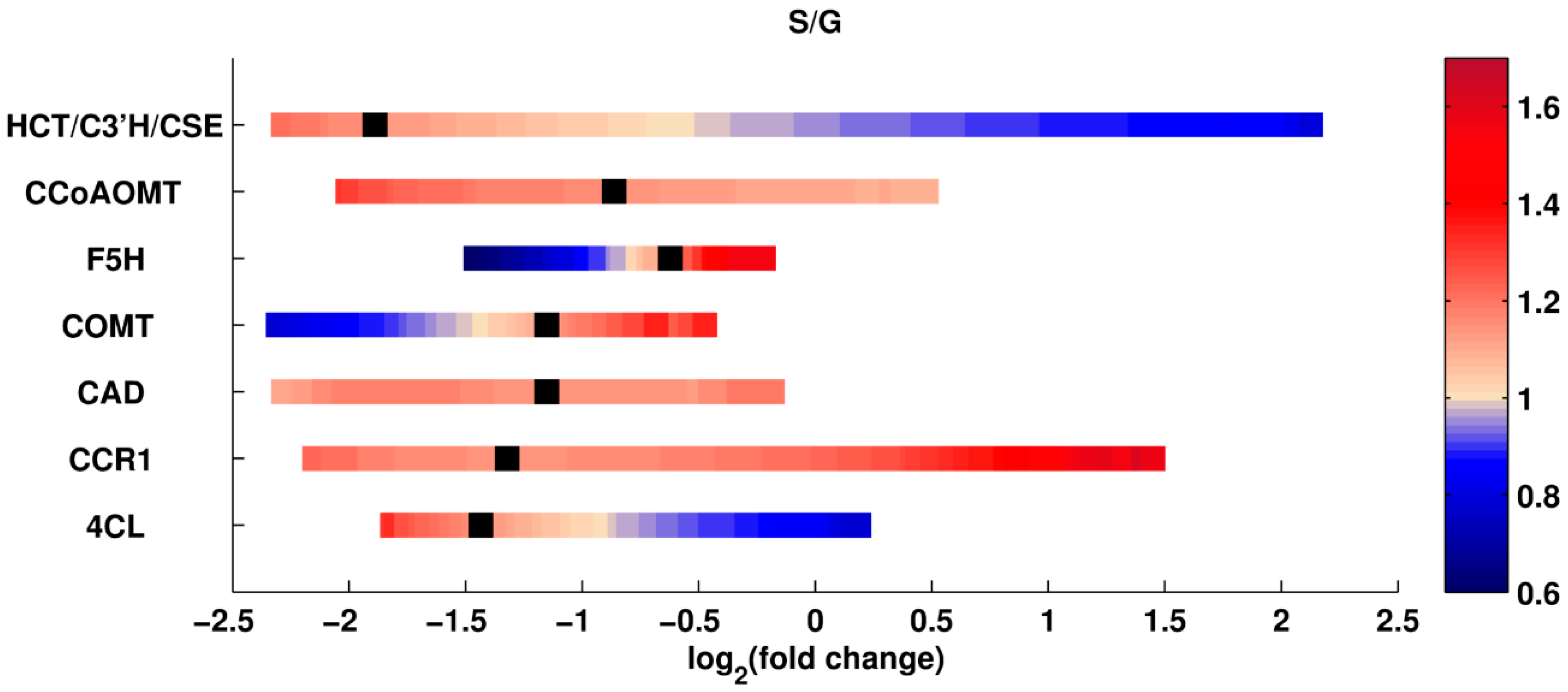
Figure 8.
Global perturbation scenarios. All seven enzymes are perturbed simultaneously. The results are broken into 12 subpanels. The subpanels in the same columns share the same S/G ratio, and the subpanels in the same row share the same total lignin. Each of the subpanels includes several columns, where each column represents a cluster of perturbation vectors that are sorted based on the distance from the wild type. Cluster c1 in each subpanel is the closest perturbation scenario to the wild type. The grey scale represents the distance from the wild type, and the red/blue spectrum shows the increase/decrease in pathway enzyme. White represents the wild type, therefore, no change in the enzyme.

Figure 9.
Clusters of results in matrix subpanels of Figure 8.
Figure 9.
Clusters of results in matrix subpanels of Figure 8.
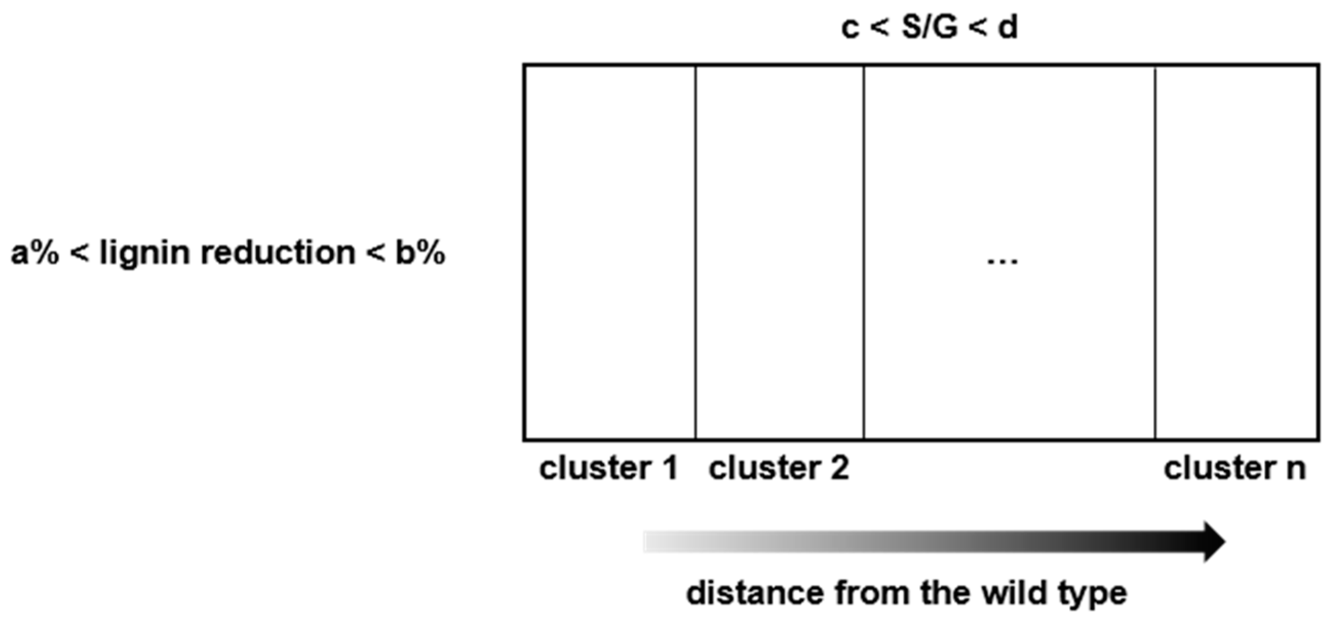
© 2017 by the authors. Licensee MDPI, Basel, Switzerland. This article is an open access article distributed under the terms and conditions of the Creative Commons Attribution (CC BY) license (http://creativecommons.org/licenses/by/4.0/).
Share and Cite
MDPI and ACS Style
Faraji, M.; Voit, E.O. Improving Bioenergy Crops through Dynamic Metabolic Modeling. Processes 2017, 5, 61. https://doi.org/10.3390/pr5040061
AMA Style
Faraji M, Voit EO. Improving Bioenergy Crops through Dynamic Metabolic Modeling. Processes. 2017; 5(4):61. https://doi.org/10.3390/pr5040061
Chicago/Turabian StyleFaraji, Mojdeh, and Eberhard O. Voit. 2017. "Improving Bioenergy Crops through Dynamic Metabolic Modeling" Processes 5, no. 4: 61. https://doi.org/10.3390/pr5040061
Note that from the first issue of 2016, this journal uses article numbers instead of page numbers. See further details here.