A General State-Space Formulation for Online Scheduling


Department of Chemical and Biological Engineering, University of Wisconsin-Madison, Madison, WI 53706, USA
*
Author to whom correspondence should be addressed.
Processes 2017, 5(4), 69; https://doi.org/10.3390/pr5040069
Submission received: 2 October 2017
/
Revised: 29 October 2017
/
Accepted: 2 November 2017
/
Published: 8 November 2017
(This article belongs to the Special Issue Combined Scheduling and Control)
Abstract
:We present a generalized state-space model formulation particularly motivated by an online scheduling perspective, which allows modeling (1) task-delays and unit breakdowns; (2) fractional delays and unit downtimes, when using discrete-time grid; (3) variable batch-sizes; (4) robust scheduling through the use of conservative yield estimates and processing times; (5) feedback on task-yield estimates before the task finishes; (6) task termination during its execution; (7) post-production storage of material in unit; and (8) unit capacity degradation and maintenance. Through these proposed generalizations, we enable a natural way to handle routinely encountered disturbances and a rich set of corresponding counter-decisions. Thereby, greatly simplifying and extending the possible application of mathematical programming based online scheduling solutions to diverse application settings. Finally, we demonstrate the effectiveness of this model on a case study from the field of bio-manufacturing.
1. Introduction
Scheduling plays an important role in all industrial production facilities [1]. Contingent on the scale of operation, optimization based scheduling methods can even achieve multi-million dollars increase in profits [2]. Thus, considerable effort has been devoted towards developing optimization models that accurately represent the decision making flexibility in these facilities [3]. Maravelias (2012) [4] provides a unified notation and a systematic framework for the description of chemical scheduling problems. Further, significant advances in solution methods, now enable us to solve small size scheduling problems. For example, a highly constrained scheduling instance over a network of 8 processing units, 19 tasks, and 26 materials, with a realistic scheduling horizon of 2 weeks, was shown to be solved to optimality in less than 1 min on an ordinary office computer [5]. Thus, being able to generate and revise schedules in an online fashion, so as to account for new information and disturbances, is very much a reality now. The Dow Chemical Company has already adopted online scheduling in many of its production facilities [6,7,8].
Scheduling models, as have been developed till now, were not necessarily designed with an emphasis on being natively ready for implementation in an online scheduling setting. Thus, the online framework utilizing a model had to be tailored to that specific model, and required many ad-hoc (heuristic) adjustments to be able to represent and resolve a disturbance to the schedule [9,10,11,12,13,14,15,16,17,18,19,20,21,22,23]. The introduction of the state-space idea to chemical production scheduling alleviated many of these issues that arose from having to make ad-hoc adjustments [24].
In this work, we present a generalized and extended state-space model which is suitable for implementation in an online scheduling setting. Further, we propose a new scheme for updating the state of the process, as well as an overall formulation to enforce constraints (through parameter/variable modifications), based on feedback information, on future decisions. Although here, we focus on expanding the modeling scope, it is important to point out that once a model has been adopted, there are still many other factors which influence the performance of an online scheduling method [25]. These factors are: the online optimization horizon length, the re-computation trigger and its frequency if periodic, allowable changes from one online iteration to the next, any added constraints (e.g., terminal constraints), and the modeling of uncertainty (deterministic vs. stochastic optimization) [8].
This paper is structured as follows. In Section 2, we present a brief background on chemical production scheduling and discuss the state-space model of Subramanian et al. [24]. In Section 3, we present a reformulated state-space model, based on a new convention, and showcase the generalizations on it one at a time. In Section 4, we present the final integrated model, with all generalizations present simultaneously, which requires more than simply concatenating all the individual generalizations together. Finally, in Section 5, we demonstrate the applicability of our proposed new model to a case study taken from the field of bio-manufacturing. Throughout the text, we use lower case Latin characters for indices, uppercase Latin bold letters for sets, uppercase Latin characters for variables, and Greek letters for parameters.
2. Background
In this section, we present the necessary background to be able to follow through the new general state-space model that we propose in this paper. Here, first, we layout the general problem statement, a standard problem representation framework, and briefly describe model classification, and solution methods. For a detailed discussion, the reader is referred to the following review papers [1,3,4,26]. Second, we show a mixed integer linear programming (MILP) based widely adopted scheduling model. Third, we describe the typical state-space formulation adopted in model predictive control (MPC) technology. Finally, we provide a short overview of the state-space based scheduling model pioneered by Subramanian and co-workers [24,27,28].
2.1. Chemical Production Scheduling
2.1.1. General Problem Statement
The general scheduling problem can be stated as follows. Given:
- (i)
- Production facility data (e.g., unit capacities and connectivity),
- (ii)
- Production recipes (e.g., processing times and mixing rules),
- (iii)
- Production costs (e.g., material holding costs),
- (iv)
- Material availability (e.g., raw materials delivery amounts and dates),
- (v)
- Resource availability (e.g., maintenance schedule and utility levels), and
- (vi)
- Production targets or orders with due-times;
scheduling seeks to find:
- (i)
- Number and the associated processing-sizes of the needed tasks,
- (ii)
- Assignment of these tasks to processing units, and
- (iii)
- Timing (or just the sequence) of these tasks on the assigned units;
so as to meet production targets at minimum cost, or to maximize profit if production beyond the given target is allowed. Apart from minimization of cost, or maximization of profit, the objective can also be minimization of makespan, or minimization of earliness, or any other suitable objective for the considered application. In general, several processing characteristics and constraints could also be present such as sequence dependent changeovers, setup times, storage constraints, time-varying utility costs, etc. [1,3].
2.1.2. Problem Representation
Before a scheduling problem can be solved, we need an abstract framework to represent the different elements of the problem, viz., the production facility, the associated production recipe, etc. The state task network (STN) enables this representation [29]. Under this representation, tasks are carried out on units (equipment), and they transform materials (states) from one to another. Apart from the material to be processed and the equipment to process these materials on, these tasks can also require resources, such as, utilities, manpower etc. Another popular framework, is the resource task network (RTN) [30]. In contrast to STN, in which materials, units, and utilities are treated as different from one another, in RTN, these are treated at par, all termed together as resources. We use the STN representation in this paper, but the general modeling ideas presented are also easily adaptable to the RTN representation.
The STN representation primarily comprises of tasks , units , and materials . The set of tasks producing/consuming material k are denoted by ; task i consumes/produces material k equivalent to mass fraction of its batch-size ( for consumption and for production). The subset of tasks that can be carried out on unit j are denoted by ; The processing time of task i, when executed on unit j, is denoted by . On any given unit, only one task can be performed at a time with its batch-size between lower () and upper capacities (); the associated fixed and proportional production costs of carrying out task i on unit j are and respectively. Feed, intermediate, and product materials are denoted by //; there are possible incoming deliveries () and outgoing orders () at certain times for selected materials; the selling price, inventory cost, and backlog cost of material k are , , and , respectively.
In Figure 1, we see a process network’s STN representation comprising of 4 material nodes (circular) labeled M0-M3 and 4 task nodes (rectangular) labeled T1-T4. Arcs connect task nodes with corresponding input/output material nodes. Tasks can be carried out in compatible units and could require utilities. Task-unit mapping and task batch-size capacities () are also shown here. Material prices () are shown adjacent to the material nodes.
2.1.3. Model Classification
Scheduling models can be classified on the basis of (i) optimization decisions; (ii) modeling elements; and (iii) modeling of time [4]. Models that employ a time-grid are either continuous time or discrete time models. In discrete time models, the fixed time-grid spacing is denoted by . Events can take place only at these grid time-points. Thus, all time-related parameters are rounded in a conservative direction, such that the resulting schedule computed using these new parameter values is feasible even for the original parameter values. Hence, processing times and raw material delivery dates are rounded up, while due dates are rounded down so as to match with an integer multiple of .
Even though, having a discrete time-grid introduces the above approximation error, discrete time models have several advantages over continuous time-grid models. For example, accounting for utility consumption, inventory and backlog costs, time varying prices, or time-dependent resource availability introduces non-linearities in continuous time models, but not so in discrete time models [26]. Furthermore, discrete time models are, in general, at least as effective as continuous time models, and in fact are better suited for large scale problems with several additional processing features [31]. In this work, we employ a discrete time-grid for our state-space model.
2.1.4. Solution Methods
To tackle the computational challenge of MILP scheduling models, several solution methods have been proposed: (1) tightening methods based on preprocessing algorithms and valid inequalities [32,33,34,35,36,37,38]; (2) reformulations [5,37,39,40,41]; (3) decomposition methods [42,43,44,45,46,47]; (4) heuristics [19,48,49,50]; and (5) hybrid methods [51,52,53,54,55]. Finally, parallel computing has been utilized to obtain faster solutions [56,57,58].
2.2. Scheduling MILP Model
The discrete time STN MILP scheduling model modified from Shah et al. (1999) [59] comprises of Equations (1)–(6). Time is represented by index . Binary variable , when 1, implies task i is starting on unit j at time t. Variable denotes its batch-size. The assignment constraint (Equation (1)) ensures only one task can be executed on a unit at a time.
Equation (2) ensures that the batch-size of a task, if initiated, is within its upper and lower bounds.
, which is the variable denoting inventory of material k during time-period , is calculated in Equation (3) as a balance of production/consumption and outgoing ()/incoming () shipments.
Equation (4) couples the outgoing shipment variable with demand, , for material k at time t. Backlog variables, , denote pending demand during time-period , and are penalized in the cost minimization objective function (Equation (5)).
Finally, the domain of all the variables is restricted via Equation (6):
2.3. Standard form of State-Space Models
State-space model formulations have been useful, alongside frequency domain models, in process control [60,61,62,63,64]. Now, as optimization based control and economic MPC are becoming the new standard, state-space models have become ubiquitous [65,66]. In the most general form, a state-space based model can be written as ; where x are the states, u are the manipulated inputs, and d are the disturbances. The function is not theoretically restricted to the class of linear functions, but is typically approximated as linear due to computational tractability considerations. The linear difference equation form for yields the model as:
where, A, B, and are state-space matrices and t is the index for time. The states x need not be associated with a physically identifiable entity in the plant. Some can have a direct physical meaning, while others can be artificial (e.g., augmented) constructs so as to enable the modeling exercise. The output (measurements y) is related to the states and inputs as , where can be non-linear, but is typically linear (e.g., , where C and D are coefficient matrices). The control optimization model has to follow the plant physical constraints and any other imposed constraints due to operational strategy (e.g., for environmental concerns) or those that enable better closed-loop properties (e.g., economics and stability). These constraints, when linear, can take the general form:
where, , , and are the coefficient matrices of the states, inputs, and disturbances, respectively. If there are any equality constraints, these can also be represented as two opposite inequality constraints, so as to conform to the general form (Equation (8)). For example, the following constraints are equivalent:
Thus, any equality constraints that we propose from here on, can be easily converted to the general inequality form through the use of the above trick. Finally, the objective function takes the form:
where N is the number of discrete time-points in the online optimization horizon.
A wealth of literature focuses on the closed-loop properties of the aforementioned iterative control methods, with novel and most recent results, specifically, in presence of discrete inputs, discussed in Rawlings and Risbeck (2017) [67].
2.4. Scheduling State-Space Model
Motivated by process control approaches, Subramanian et al. (2012) [24] proposed a state-space model (Equations (5) and (11)–(16)) for the chemical production scheduling problem. For brevity, we present the formulation for constant batch-sizes (). There are two distinct features of this model. First, the “complete status” of the plant can be interpreted solely from the variables (states) at that moment in time. This is made possible by lifting past actions/inputs (the task start binary variables, ) which have a lagged effect on the “current status" of the plant. Second, observed uncertainties are treated as disturbances, and represented as parameters in the model equations. These two features, together, allow for the model to be kept identical in each online scheduling iteration without any ad-hoc adjustments (due to observation of uncertainty). Thus, the model is in “online ready” form. In addition, due to the use of the state-space formulation, which is popular in process control models, this model also happens to be a very suitable candidate for integration of scheduling and control [68].
To enable lifting of inputs, new task-states (variables) are defined. Although this increases the number of variables in the model, it is matched by an equal increase in the number of equations (the lifting equations, Equations (11) and (12)). Thus, no new degrees of freedom are introduced. When the task starts, n is zero (, Equation (11)), and when the task finishes, n equals the processing time of the task (). To express task delay and unit breakdown disturbances, new parameters and are defined, respectively. , when 1, denotes a delay of h in task i during time-period , where , as defined in Section 2.1.3, is the granularity of the discrete time-grid. , when 1, denotes break-down of unit j while executing task i during time-period . For ease of presentation, we assume from here on that h.
In the absence of delays or breakdowns, the lifting equations effectively represent the relation: . The lifted variables are defined only till , because a “look-back” beyond that value of n is not needed. The effect of past inputs, for , is already, indirectly, contained in the inventory and backlog variables and . The lifted states, , are augmented to the future states (see Figure 2).
In the assignment constraint (Equation (13)), parameters and are included, to ensure that the unit appears to be busy, and no new tasks can be started, when there is a delay or breakdown observed at a time when a task is about to finish. Additionally, for multi-period breakdowns, parameter is made 1, where IT is a fictitious “idle task”, with , that keeps the unit busy through the duration of the multi-period breakdown.
In inventory balance (Equation (14)), and are parameters that denote material handling loss during consumption and production of material k, respectively. When a delay or breakdown is observed at the end of a task, the terms and , which are subtracted from , prevent erroneous multiple counting of the material amount produced by that task.
In the backorder balance (Equation (15)), denotes demand disturbance.
Finally, Equation (16) shows the bounds on the variables present in the model.
Next, we describe the online update step, i.e., how information is carried over from one online iteration to the next. Since the scheduling horizon is advanced by 1 h (the model is kept identical), the state at (initial condition) for the next iteration is matched with the state at of the previous iteration. This is shown in Figure 2, and achieved through the online “update equations” (Equations (17)–(19)), in which denotes the iteration number. Variables , , and for which represent lifted task-states, are assigned fixed values through the update step. But, , which represents degrees of freedom to start new tasks at , is not fixed. This is identical to how the online updates are performed for the no disturbance case [25]. However, since, here we are dealing with the case where disturbances can be present, the disturbance parameters (, , , , and ) are also assigned appropriate values to reflect the observed disturbances. However, these parameters do not participate in the update equations. These influence the prediction of states, for , in the online iteration .
Figure 3A,B, show the evolution of task-states when a 2 h delay is observed right after a task starts and just before a task is about to finish, respectively. The 2 h duration of this multi-period delay is known immediately in iteration . However, the model formulation also does allow for representing the observation of consecutive, possibly independent, 1 h single-period delays, one at a time in succeeding iterations. These collectively, in hindsight, appear to be a single multi-period delay, but are actually not.
It is quite evident, that n, now in the presence of delays, loses its physical meaning of denoting how much progress has been made on the task. For example, for the task in Figure 3A (iteration ), due to the 2 h delay, the task-states evolve as , instead of the more intuitive . Similarly, in Figure 3B (iteration ), the task-states evolve as , instead of the more intuitive . All that can be said now is that when , the task has just started at time t, and when and simultaneously, then the task has finished. As we will show in Section 3.1, we overcome this limitation by introducing a new convention to map observed disturbances to the disturbance parameters, and hence, are able to preserve the physical meaning of n, even when disturbances are present (see Figure 4).
Figure 5A,B, show the evolution of task-states when a breakdown just before is observed and is known to have a 2 h unit downtime (for repairs), right after a task starts and just before a task is about to finish, respectively. Given the observation of breakdown, we would expect intuitively, and unlike what is shown in Figure 5A,B, that none of the task-states are active for the green task at . We show how this is achieved through the new model discussed in Section 3.1 (see Figure 6).
3. Modeling Generalizations
In Section 3.1, we present a new state-space model formulation that differs, from the state-space model of Subramanian et al. (2012) [24], in the convention that is followed for mapping observed disturbances to the disturbance parameters. Although both models are accurate, this new convention ensures that the task-states, in the presence of disturbances, follow a more intuitive notation. Specifically, the meaning of n as the progress of a task, is maintained. In addition, we define several new parameters to systematically account for disturbances.
In Section 3.2, we show how to handle fractional delays and unit downtimes (due to unit breakdowns). In Section 3.3, we expand the scope of the model to account for variable batch-sizes. Thereafter, in Section 3.4, Section 3.5, Section 3.6, Section 3.7, Section 3.8 and Section 3.9 we present generalizations that can be applied to the state-space model, one at a time. Afterwards, in Section 4, we present the final model equations with all generalizations present simultaneously. As we will see in that section, for all the generalizations to work in the presence of each other, a few more modifications are necessary.
3.1. New Basic Formulation
The new state-space model relies on a comprehensive update step of the task-states, in between the online iterations, to promptly reflect the delays and breakdowns in the task-states. The inventory and backorder update stay the same (Equations (18) and (19)) as in the model of Subramanian et al. (2012) [24]. The task-states update is modified from Equation (17) to Equations (20) and (21).
The parameters which, if 1, represent a 1 h delay in task with progress status n. Note the dot (·) instead of the hat (∧) on the symbols of these parameters. Since these parameters are exclusively for the update step, and do not directly participate in the optimization model, these need not be indexed by time—neither (iteration ) nor t (iteration ). Similarly, denotes a breakdown of unit j on which task i with progress status n was running. is a new binary variable, defined for all time-points, which, when 1, captures the information about delays in a task with progress status , i.e., when the task gets delayed right after it starts. The use of this variable, in Equations (22) and (23), will become clear when we discuss the optimization model. We also define a new parameter , which, when 1, denotes the unit is unavailable for the time-period . This parameter participates in Equation (25).
For a multi-period delay of h, in task i on unit j, in addition to , parameters are activated for . For unit breakdowns with downtime duration of h, in addition to , parameters, are activated for . Thus, single-period delays do not result in activation of any parameters, but single-period breakdowns require activation of .
Having described the update step, we now describe the optimization model. In this model, the lifting equations consist of Equations (22)–(24).
When there is a h multi-period delay in a task with progress , the update step assigns and . This ensures that stays activated for next () h, but with , i.e., the task is not erroneously interpreted as a new task start. If there are no delays, then, through Equations (21) and (22), and any new task that starts with , through Equation (23), results in . Equation (23) is a constraint that we impose on the inputs () given the states ( and ), and if needed can be converted to inequality form through use of Equation (9). Variables are either fixed () by the update step or are equated to the delay parameters in the optimization model, hence, can be declared as free variables with no explicit bounds.
The assignment constraint (Equation (25)) includes the parameter to account for unit downtime. Additionally, it contains the variable on the left-hand side, and not variable , to correctly account for the unit being busy, specifically, when a delay in a task with progress is observed.
The inventory balance, Equation (26), in contrast to Equation (14), does not require any corrective delay or breakdown terms. This is because, for any task, the states (task-start) and (task-end), even if delays or breakdowns are observed, are active only at most once.
3.2. Fractional Delays and Unit Downtimes
In Figure 4 and Figure 6, we showed the cases where delays and unit downtime are integer multiples of time-grid spacing . Additionally, the unit breakdown was assumed to take place at almost the time-point t, i.e., very close to an integer multiple of . However, if is not very small, then these assumptions may not be good. Given any fractional delays (), downtimes (), or unit breakdown time (), we need an appropriate scheme for the (online iterations) update step, to ensure realistic rounding of these to integer values, so as to keep the task-finish and unit-availability times, in sync with the discrete time-grid. A single task can have multiple separate delays, hence, we index the delay time with index r (recurrence), i.e., . A breakdown, however, can occur only once, at , following which, the unit downtime, , starts.
For the first delay, a rounded up value is applied in the update steps, i.e., the delay is assumed to be . For every additional th delay, the difference, , dictates how much additional, integer , delay is applied in the update steps. Figure 7A shows a numerical example for fractional delays.
When a unit breaks down, the parameter is always activated, so as to suspend the running task. The key challenge is to identify, for how many next time-points the unit would be unavailable. This dictates, if, and how many, parameters are activated. This is done as follows. On breakdown, the unit becomes unavailable from to (in iteration , ). Hence, all that span integer multiple of , are activated. This also means, if , none of the are activated, i.e., the unit breaks down and comes back online before the immediate next time-point. This is illustrated in Figure 7B.
3.3. Variable Batch-Sizes
To account for variable batch-sizes, we define variables, which denotes the batch-size of the task that just starts, for lifted task batch-size states, and to represent batch-size of task that is delayed with progress status . We define parameters and that participate in the update steps and these denote the batch-size of the task delayed and suspended due to unit break-down, respectively. Further, we define parameter for the optimization model.
It might appear in Equation (30) that when , nothing prevents from also erroneously taking on a positive value. This was not an issue in Equation (23) because the and variables there were binary. However, Equation (2) ensures that can only take a non-zero value when . Since, through Equation (23), , whenever , also takes value 0. The update steps ensure that and can only be non-zero simultaneously.
The inventory balance (Equation (32)) now incorporates the new batch-size variables, and , rather than the task-state binary variables ( and ) which was the case in Equation (26).
Finally, the variable bounds are as follows:
The update step comprises of Equations (18)–(21), (27) and (28), and the optimization model consists of Equations (2), (5), (15), (22)–(25) and (29)–(33).
Remark: In principle, we can completely avoid defining the new parameters , , , and variable by reformulating Equations (27)–(31), so as to only use parameters , , , and variable . For example, Equation (31) can be reformulated to Equation (34).
Since, Equation (34) entails the multiplication of variables with parameters, by itself, it is an acceptable alternate linear formulation. However, when task termination is allowed as a scheduling decision (Section 3.7), this reformulation results in bi-linear terms which are undesirable. Thus, we indeed define the new parameters , , , and variable , and use Equations (27)–(31) in their native form without the simplifying reformulation discussed in this remark.
3.4. Robust Scheduling: Batch-Sizes
In many applications, it can be prudent to schedule batches bigger than what are needed to just satisfy the nominal demand. This can be, for example, due to the possibility of seeing a demand spike, or to pro-actively compensate for typical material handling losses when a batch finishes. To do so, the parameter in material inventory balance (Equation (35b)) can be substituted by a scaled down value (), where . This results in bigger batches starting, since the model now under-predicts the yield of materials from any given batch-size. In order to, however, correctly account for the actual inventory resulting from the finishing of a task, the nominal value of is used at , along with any yield-loss or material handling loss disturbance (Equation (35a)). As it can be seen in Figure 8, which is a simple illustration of this modeling generalization, as the iterations progress, a task-finish-state eventually hits , yielding the large yield proportionate to the true (nominal) value of . Now, if there are any material handling losses (), they can be subtracted from the true yield (in Equation (35a)). It is worth noting that, although and are defined for all time-points, they are possibly active only at , if the corresponding uncertainty is observed. Hence, these parameters can be, in principle, dropped from Equation (35b).
We can write the above two equations, compactly together, as follows:
where
3.5. Robust Scheduling: Processing Times
Uncertainty in the processing times is very common in scheduling [69]. A popular approach to proactively manage this uncertainty is to robustify the schedule by adding a delay buffer to each task’s processing time [70]. Once this robust schedule has been computed, it is advantageous to adjust it online, by taking into account the feedback on actual finish times of the tasks [71]. In discrete-time models, this has been typically done using ad-hoc adjustments in between the online iterations. To the best knowledge of the authors, there is not yet a systematic way to be able to naturally handle this adjustment within an optimization model.
We show here how we can extend the state-space model to produce robust schedules, from a processing time point of view, and yet seamlessly allow for tasks to finish, after they have been running for their nominal processing times plus the delays. We define a new parameter , which denotes the conservative processing time of the tasks (). Thereafter, we modify the lifting (Equation (24) modified to Equations (38a), (38b) and (31) modified to Equations (39a) and (39b)), assignment (Equation (25) modified to Equations (40a) and (40b)), and inventory balance equations (Equation (32) modified to Equations (41a) and (41b)), such that the nominal value of processing times () is employed at , and the conservative value () is employed for . No other model or update equations are modified. An illustration is given in Figure 9.
The lifting equations, Equations (38b) and (39b), contain variables , which are not coupled back to any variables at . These variables must be fixed to zero, otherwise, the optimization can assign these variables a spurious value so as to erroneously generate inventory (in Equation (41b) through variables ).
We can write the above equations, compactly together, as follows:
where
Finally, please note that in this approach, as can be seen in Figure 9B (iteration ), an a priori fixed buffer time () is added to the task duration, irrespective of whether delays have already been observed (during the execution of the current task). It can be argued that the buffer was meant to absorb the actual delays, and hence, should be cut back for tasks that actually get delayed. This is a fair critique. However, owing to feedback, the true task-finish is accounted for (see Figure 9A iteration ), and there is no wasted equipment time due to the unused buffer, which otherwise results in idle time in static robust scheduling approaches.
3.6. Feedback on Yield Estimates
The material handling loss () disturbance parameters can be used to represent yield losses as well, but these parameters are assigned a value only at , i.e., when a task actually ends and a material handling loss is observed. In many applications, the actual yield of a task can, in fact, be estimated during the task’s execution, and does not always come as a surprise when the batch finishes. To incorporate the information about anticipated yield loss in future, these parameters can be assigned values for . However, this information has to be then carried over from one iteration to the next, with corresponding decrement in the t index of these parameters to reflect the shifting time-grid, till the task finishes. In addition, if the task is delayed, these parameter values also have to be delayed. This requires cumbersome mechanisms to handle this information in between the online iterations.
Adapting the state-space model to lift the yield-loss information forward provides a much more natural way to handle this feedback. Thus, we define a new free variable , which is analogous to the batch-size variable , but, as we can see in Equation (47), when the task finishes, instead of adding to, it subtracts from the inventory.
Thus, in a way, this new variable can be thought to be the negative counterpart of the batch-size variable. The yield loss can also be delayed by use of the parameters and so as to stay in sync with the task-finish time, or nullified in case of a unit breakdown through the parameter . This is achieved using the update steps (Equations (48) and (49)) and the model lifting equations (Equations (50)–(52)).
is a parameter the denotes the “additional” yield loss observed (anticipated) in that iteration (). When delays and yield losses are observed simultaneously, then the parameters and take the value , i.e., the total yield loss up to and including in iteration .
Please note that there are no variables in Equation (51). If these variables were to be present, they would have to be fixed to zero. Otherwise the optimization itself can spuriously assign non-zero values to these variables, such that the intended true batch-size is .
3.7. Task Termination
In the update step (Equations (20), (21), (27) and (28)) we made an implicit assumption that past decisions (task-states with at ) are fixed. In general, more decisions from the previous iteration can be considered fixed or the deviation from them penalized in the current iteration. This has been suggested in the literature to reduce schedule nervousness [23,72,73].
However, to the best knowledge of the authors, no model to date considers canceling/terminating tasks already underway, as an optimization decision. This is surprising, given that whenever is needed, this would be a natural decision for a human scheduler. For example, to prioritize processing for a new rush order, an unfinished process unrelated to this rush order may need to be terminated. Other routine possibilities for task termination are excessive delays or yield losses, as is commonly the case in bio-manufacturing [74,75]. This decision to terminate should be an outcome of the online optimization so as to best react to the observed disturbances or new information. We define task termination as a “willful” decision to discontinue a task. This is in contrast with task suspension, which is a “forced” discontinuation of a task as a result of a unit breakdown or loss of utility support. Since, preemption is not customary in chemical processes, we assume a total loss of output of a task that is terminated. This is in agreement with how the output of task suspensions is treated.
This termination of tasks can be achieved by “softening” the initial conditions (task-states at ) in an online iteration. We introduce a new binary variable, , which, when 1, denotes termination of task i, on unit j, which has run-index n. Since, all variables values for iteration are now a parameter for iteration , we can write the following linear equations to achieve this softening:
Hence, the update equations (Equations (20), (21), (27) and (28) modified to (53)–(56)) now become part of the model. The update equations for inventory (Equation (18)) and backlog (Equation (19)) stay unmodified, and are not softened.
If we had no disturbances, just softening the initial task-states would have sufficed. However, when we have delays, we have to also ensure that we appropriately nullify the effect of delay parameters, which have been already assigned a value at the start of an iteration (optimization). Thus, wherever the delay parameters appear, we multiply these with . Since the coefficients of the terms are the delay parameters, when there is no delay, these terms are also, consequently, absent. Parameters , , , and are always zero, hence, variables do not participate in the model. A unit breakdown implicitly disrupts a task, hence, in such a situation, the question of termination does not arise. Overall, the lifting equations are modified to Equations (57)–(60) with Equations (23) and (30) remaining unchanged.
We do not index variable with time (t), because it serves no purpose to terminate a task in future (). If a task is already under execution and has to be terminated in the future for some reason, it is always better to terminate it right away ().
In addition to including a cost associated with task termination, , in the objective, we can also enforce a pre-specified unit downtime () following every task termination, by including a summation term in the assignment constraints for that many time-points:
We can write the above two equations, compactly together, as follows:
where
An added advantage of the compact form, is that the unit downtime can now be a function of the task that was terminated, i.e., is indexed by i as well, and not just j.
To systematically account for unit downtime resulting from task-termination in a previous iteration, i.e., if , the parameter has to be activated for in iteration . Thereafter, in each subsequent iterations, the downtime is decremented by 1, and the parameter appropriately activated for the corresponding time-points. Alternatively, we can define a new binary variable and lift it, to keep the unit deactivated for the remaining downtime in subsequent iterations. The new variable, which would be subtracted on the right hand side of Equations (61a) and (61b), in lieu of , can be thought of as the unit unavailability variable.
3.8. Post-Production Storage in Unit
Kondili et al. (1993) [29] proposed a formulation for “hold” tasks, which are dummy tasks that can be used to model storage of materials in a processing unit, while waiting to be unloaded. This is especially important for production facilities that follow a no intermediate storage (NIS) policy for certain materials. In the network shown in Figure 1, task T4 is a hold task. The purpose of this task is to keep material M3 residing in unit U3. So as to ensure that the hold task can only store material in a unit that it was originally produced in, we write the state-space version of the original constraint proposed by Kondili et al. (1993) [29] in Equation (64).
where is the set of hold tasks. When multiple materials are produced in a unit, here we assume that the corresponding hold task emulates the simultaneous storage of all these materials in the unit. The mass-coefficient then dictates in what proportion are the materials released from the unit. If only a certain individual material is held, and the others unloaded, the term is substituted with , and the constraint is written only for that material k which is held. Further, for a perishable material, ; that is, a fraction of the material is lost (perishes or deactivates) when held.
3.9. Unit Capacity Degradation and Maintenance
In many processes, such as polymerization reactions, or purification processes, it is not uncommon for the unit capacity to “degrade” after a task has been processed on that unit [76,77,78,79,80,81]. This can be, for example, due to residue formation (e.g., scaling) or impurity accumulation (e.g., membrane pore blockages). Some degradation is gradual and predictable, while some degradation may occur suddenly and unexpectedly.
To model unit degradation, we define a new non-negative variable, , which denotes the capacity of the unit j, to perform task i that starts at time t. For an un-degraded unit, is initialized to the value . This variable value is passed over from one iteration to another, through the update equation:
A new disturbance parameter, , which when negative, represents extent of sudden (unexpected) partial loss in unit capacity. Conversely, a positive value represents renewal of unit capacity. This positive value could be, for example, a result of installing a new repaired unit in place of an old unit that broke down.
Through Equation (66), we define a balance on the unit capacity. is a parameter that denotes the gradual degradation in capacity of unit j to perform task i, due to execution of task on that unit. is either negative or zero.
The degraded unit can be typically restored to its full capacity through a maintenance task (e.g., cleaning), which we denote with the abbreviation MT. We define as a set of maintenance tasks, and as a set of units which can degrade, and consequently, need a corresponding maintenance task. Further, we add the maintenance task (MT) to the set of tasks that can be performed on unit j. The value of , the variable which we define below, dictates the restored capacity due to completion of a maintenance task.
Like any conventional task, the maintenance task has a start binary () associated with it, which is appropriately lifted. The assignment equation (Equation (25)) ensures that the maintenance task can only run when the unit is not running any other task. Since the maintenance task does not consume or produce materials, the conventional batch-size of this maintenance task, is fixed to zero. Instead, we define a new type of batch-size, , specific to the purpose of this task, which we term as the maintenance-size. Since we assume that only one kind of a maintenance task exists for every unit, the index i in this maintenance-size variable is not MT. This variable denotes, how much capacity to perform task i is restored, when maintenance is performed on unit j. This variable is also lifted, similar to the batch-size variable, and can be delayed or suspended due to breakdowns. Similarly, the parameters , , and denote the maintenance-sizes of the maintenance task corresponding to capacity restored to perform task i. The update equations associated with this variable are:
The model equations, for lifting, are:
The batch-size of new tasks is upper bounded by the unit capacity variable (Equation (72)). This ensures that only smaller batches can now be processed if . If a task just finishes, the restored or degraded capacity due to that is also accounted for while upper bounding the task-batchsize .
We define the maintenance task with fixed processing time (), and assume that whenever performed, the unit is restored to its full capacity (i.e., ). This requires the maintenance-size, , to be the difference between the deteriorated unit capacity (), before the maintenance starts, and the upper capacity limit (), to which the unit has to be restored to. This is achieved using Equation (73):
Finally, we specify the lower and upper bounds for variable :
and define a new parameter , which denotes the proportional cost of maintenance of a unit. The cost term, in the objective, for a maintenance task is .
4. Integrated Model
In this section, we present the complete model with all generalizations present simultaneously. For brevity, we write index in only those equations, where is also present. Everywhere else, all variables are those of the current iteration .
The update equations are Equations (18), (19), and (65). The softened update equations, which are part of the model, are Equations (53)–(56) and (75)–(78).
The lifting equations are Equations (23), (30), (51), (57), (59), (70), and (79)–(84).
where please note the use of parameter in Equations (79), (80), (82), and (84).
The assignment constraint is:
Batch-size, post-production storage, and maintenance-size constraints are Equations (2), (88), and (73) and (89).
Bounds on the variables are enforced by Equations (74) and (90)–(92).
Variables are free variables, however, through the update and model equations, they are always equated to a parameter value, hence, are not degrees of freedom. The decision variables, or in other words—the inputs from a systems perspective [24], are , and .
The objective is:
5. Case Study
Bio-manufacturing is a type of manufacturing in which molecules of interest, such as, metabolites, drugs, enzymes, etc., are produced through the use of biological systems such as living micro-organisms [82]. Several commercial sectors, rely on these, for example, pharmaceuticals, food and beverage processing, agriculture, waste treatment, etc. Furthermore, there is an increasing thrust towards finding biological routes for production of bulk chemicals [83]. The use of live systems in bio-manufacturing, however, introduces several operational challenges. These include batch-to-batch variability, parallel growth of both, the desired product as well as undesired toxic byproducts in the same batch, and possible random shocks that can lead to complete failure of a batch [75]. This makes it an interesting area for application of scheduling methods. In this section, we present an example, motivated from bio-manufacturing, to demonstrate all modeling generalizations discussed in Section 3, using the integrated model equations outlined in Section 4.
In general, bio-manufacturing processes can be divided into an upstream bio-reaction (e.g., fermentation) stage and a downstream purification stage [74]. The upstream stage typically consists of two steps: cell culture preparation in the lab and the bio-reaction. These two steps are task T1 and T2, respectively, in the network in Figure 1. The downstream purification stage typically consists of three steps: centrifugation, chromatography, and filtration. Among these three steps, chromatography takes the longest and the chromatograph columns are prone to unpredictable failures. Hence, we assume that chromatography, being the dominant step, is representative of the complete purification stage. This is task T3 in the network in Figure 1. Overall, we choose this simplified system (network) for an easier illustration of the capabilities of our general state-space model.
In our example, as features, we allow for possible delays in the cell culture preparation (T1), and small yield losses in the bio-reaction (T2), including possible substantial yield losses due to sudden cell death. Thus, we carry out robust scheduling, using a conservative processing time () for task T1 and a conservative mass-conversion coefficient (), against small yield losses, for task T2. Further, in the downstream stage, we assume that the chromatograph column (U3) loses capacity with usage, part of which is predictable. Executing a maintenance task can restore capacity on the chromatographs. To enforce the no-intermediate storage (NIS) policy for material M2, the inventory variable is fixed to zero for all time-points. Raw material, M0, is assumed to be available in an unrestricted supply, as needed. Selected instance parameter values, other than the ones already shown in Figure 1, are outlined in Table 1.
An order for 15 kg of M3 is due at the 14th hour of the day. To meet this order, online scheduling is carried out, with a horizon of 16 h, and re-optimization every 1 h, starting at the 0th hour. All optimizations are solved to optimality using default solver options in CPLEX 12.6.1 (IBM Corporation, North Castle, NY, USA) via GAMS 24.4.3 (GAMS Development Corporation, Fairfax, VA, USA), installed on an Intel Xeon (E5520, 2.27 GHz, 8 core processor) machine (Intel Corporation, Santa Clara, CA, USA), with 16 GB of RAM and Linux CentOS 7 operating system (Red Hat Inc., Raleigh, NC, USA). The schedules obtained in selected online scheduling iteration are shown in Figure 10. For the remaining online iterations, the predicted schedule is identical to the respective previous iteration (but with time-grid shift).
The nominal makespan, without any disturbances or robustification, to meet this order is 13 h. However, in iteration 0 (see Figure 10), T1 is started at , instead of , since a conservative processing time, h is in use. Further, the batch-sizes for T1 and T2 are 16.67 kg, since a conservative yield parameter () is in use for T2. This predicts production of 15 kg of M2, which through the two T3 batches, of 6.25 kg and 8.75 kg, makes 15 kg of M3.
In the next iteration, a fractional delay of 0.5 h is observed. Due to the use of a discrete time-grid with granularity h, and being the first delay for this task, this is rounded up to 1 h. Since, now the order is predicted to be late, the batch-sizes of T3 are revised so as to meet as much of the order as possible on time (). Going forward, no more delays are observed in T1, hence, it finishes at in iteration 3. This is because the nominal is in use at in Equations (85) and (86). Consequently, the downstream tasks are all scheduled earlier now, matching up with the initial predicted schedule in iteration 0. Thus, the conservative processing time was useful, in making T1 start earlier at 0th hour.
In iteration 4, due to sudden cell death, 90% yield loss in T2 is observed (anticipated at task finish). Hence, T2 is terminated. T1 is restarted (with conservative processing time). Since, no delays are observed through the execution of this new task T1, in iteration 6, it finishes after the nominal processing time of 2 h. Thus the start times of the downstream tasks are pulled forward by 1 h.
In iteration 9, 10% yield loss is observed (anticipated at task finish). Since, this is not substantial, T2 is not terminated. Instead, a new train of tasks is scheduled to start at to compensate for the lost yield. In iteration 11, when T2 finishes, it results in nominal yield () minus the 10% anticipated yield loss. Hence, 15 kg of M2 is produced. Thus, the new train of tasks previously scheduled, but not yet started, in iteration 9 are canceled.
In iteration 11, in addition to the gradual decline in chromatograph capacity due to usage (), which does not affect starting the next 5 kg T3 task, a sudden loss in capacity is observed (). Hence, a maintenance task (MT) is scheduled with maintenance-size . Once this maintenance is over, the pending task T3 can start. No further disturbances are observed. Consequently, the order is fully met at the 19th hour.
If task termination, conservative processing time, and conservative yield were not used, the order would have been fully met only at the 27th hour (Gantt chart not shown). Hence, using the general state-space model enabled a richer set of decision making, resulting in an overall better schedule.
6. Conclusions
We developed a general state-space model, particularly motivated by an online scheduling perspective, that allows modeling (1) task-delays and unit breakdowns with a new, more intuitive convention over that of Subramanian et al. (2012) [24]; (2) fractional delays and unit downtimes, when using discrete-time grid; (3) variable batch-sizes; (4) robust scheduling through the use of conservative yield estimates and processing times; (5) feedback on task-yield estimates before the task finishes; (6) task termination during its execution; (7) post-production storage of material in unit; and (8) unit capacity degradation and maintenance. Further, we propose a new scheme for updating the state of the process, as well as an overall formulation to enforce constraints (through parameter/variable modifications), based on feedback information, on future decisions. We demonstrate the effectiveness of this model on a case study from the field of bio-manufacturing. Through this new state-space model, we have enabled a natural way to handle routinely encountered processing features and disturbance information in online scheduling. The general features that we address are found in several industrial sectors, namely, pharmaceuticals, fine chemicals, pulp and paper, agriculture, steel production, oil and gas, food processing, bio-manufacturing, etc. The proposed model, therefore, greatly extends and enables the possible application of mathematical programming based online scheduling solutions to diverse application settings. Finally, it is important to note, that although here we presented the model using STN based representation, these generalizations can also be adapted to RTN based representation.
Acknowledgments
The authors acknowledge support from the National Science Foundation under grants CMMI-1334933 and CBET-1264096, as well as the Petroleum Research Fund under grant 53313-ND9. Further, the authors thank Ananth Krishnamurthy for fruitful discussions on bio-manufacturing.
Author Contributions
D.G. conceived the model and prepared the manuscript under the supervision of C.T.M.
Conflicts of Interest
The authors declare no conflict of interest.
Abbreviations
The following abbreviations are used in this manuscript
| MILP | mixed integer linear program |
| MPC | model predictive control |
| RTN | resource task network |
| STN | state task network |
| HOLD | hold (storage) task |
| MT | maintenance (cleaning) task |
Nomenclature
| Indices/sets | |
| tasks | |
| units (equipment) | |
| materials | |
| time-points/periods | |
| tasks that can be carried out in unit j | |
| tasks producing material k | |
| tasks consuming material k | |
| hold (storage) tasks | |
| maintenance tasks | |
| units suitable for carrying out task i | |
| units which can degrade, and consequently, need a corresponding maintenance task | |
| feed (raw) materials | |
| intermediates | |
| final products | |
| Parameters | |
| fixed cost of running task i on unit j | |
| proportional cost of running task i on unit j | |
| cost of terminating task i on unit j | |
| proportional cost of maintenance task i on unit j | |
| fixed batch-size of task i executed on unit j | |
| min/max capacity on batch-size of task i executed on unit j | |
| material unloading/loading loss during production/consumption of material k | |
| selling price of material k | |
| inventory cost of material k | |
| backlog cost of material k | |
| discretization of time-grid; length of time-periods | |
| incoming shipment of material k at time t | |
| disturbance parameter denoting unit breakdown | |
| batch-size of task suspended due to unit breakdown | |
| yield-loss size of task suspended due to unit breakdown | |
| maintenance-size of maintenance task suspended due to unit breakdown | |
| dummy parameter as defined in Equation (46) | |
| dummy parameter as defined in Equation (37) | |
| dummy parameter as defined in Equation (63) | |
| yield loss in task i running on unit j, with run status n | |
| binary parameter, when 1, denotes unit j unavailable during time | |
| when negative, represents extent of sudden partial loss in unit capacity | |
| demand for material k at time t | |
| demand disturbance for material k at time t | |
| actual (fractional) time at which a unit breaks down | |
| fractional downtime in a unit | |
| fractional delay in a task | |
| rth delay in a task | |
| mass-conversion coefficient (material consumption) | |
| mass-conversion coefficient (material production) | |
| conservative mass-conversion coefficient for production () | |
| deterioration in unit capacity to perform task i, due to performing task on that unit j. | |
| online iteration number | |
| processing time of task i on unit j | |
| conservative processing time of task i () on unit j | |
| task independent unit j downtime after terminating a task | |
| task dependent unit j downtime after terminating task i | |
| , | single-/multi-period disturbance parameters denoting delay |
| , | single-/multi-period disturbance parameters denoting batch-size of a delayed task |
| , | single-/multi-period disturbance parameters denoting yield-loss size of a delayed task |
| , | single-/multi-period disturbance parameters denoting maintenance-size of delayed maintenance task |
| duration of delay or breakdown, in multiples of | |
| recurrence count of delay for a task | |
| Variables | |
| batch-size of task i on unit j | |
| lifted batch-size | |
| backlog level of material k during period | |
| capacity of unit j to perform task i during period | |
| lifted yield-loss variables | |
| maintenance-size of the maintenance task | |
| lifted maintenance-size | |
| inventory level of material k during period | |
| binary variable, when 1, denotes termination of task i, with run-status n, on unit j | |
| outgoing shipment to meet demand for material k at time t | |
| binary variable, when 1, denotes task i starts on unit j at time-point t | |
| lifted task-start variables | |
| when 1, captures the information about delays in a task with progress status | |
| the batch-size of delayed task with progress status | |
| yield-loss of delayed task with progress status | |
| maintenance-size of delayed maintenance task with progress status | |
References
- Harjunkoski, I.; Maravelias, C.T.; Bongers, P.; Castro, P.M.; Engell, S.; Grossmann, I.E.; Hooker, J.; Méndez, C.A.; Sand, G.; Wassick, J.M. Scope for industrial applications of production scheduling models and solution methods. Comput. Chem. Eng. 2014, 62, 161–193. [Google Scholar] [CrossRef]
- Kelly, J.D.; Mann, J. Crude oil blend scheduling optimization: An application with multimillion dollar benefits. Hydrocarb. Process. 2003, 82, 47–54. [Google Scholar]
- Méndez, C.A.; Cerdá, J.; Grossmann, I.E.; Harjunkoski, I.; Fahl, M. State-of-the-art review of optimization methods for short-term scheduling of batch processes. Comput. Chem. Eng. 2006, 30, 913–946. [Google Scholar] [CrossRef]
- Maravelias, C.T. General framework and modeling approach classification for chemical production scheduling. AIChE J. 2012, 58, 1812–1828. [Google Scholar] [CrossRef]
- Velez, S.; Maravelias, C.T. Reformulations and branching methods for mixed-integer programming chemical production scheduling models. Ind. Eng. Chem. Res. 2013, 52, 3832–3841. [Google Scholar] [CrossRef]
- Wassick, J.M.; Ferrio, J. Extending the resource task network for industrial applications. Comput. Chem. Eng. 2011, 35, 2124–2140. [Google Scholar] [CrossRef]
- Nie, Y.; Biegler, L.T.; Villa, C.M.; Wassick, J.M. Discrete Time Formulation for the Integration of Scheduling and Dynamic Optimization. Ind. Eng. Chem. Res. 2015, 54, 4303–4315. [Google Scholar] [CrossRef]
- Gupta, D.; Maravelias, C.T.; Wassick, J.M. From rescheduling to online scheduling. Chem. Eng. Res. Des. 2016, 116, 83–97. [Google Scholar] [CrossRef]
- Cott, B.J.; Macchietto, S. Minimizing the effects of batch process variability using online schedule modification. Comput. Chem. Eng. 1989, 13, 105–113. [Google Scholar] [CrossRef]
- Kanakamedala, K.B.; Reklaitis, G.V.; Venkatasubramanian, V. Reactive schedule modification in multipurpose batch chemical plants. Ind. Eng. Chem. Res. 1994, 33, 77–90. [Google Scholar] [CrossRef]
- Huercio, A.; Espuña, A.; Puigjaner, L. Incorporating on-line scheduling strategies in integrated batch productioncontrol. Comput. Chem. Eng. 1995, 19, 609–614. [Google Scholar] [CrossRef]
- Kim, M.; Lee, I.B. Rule-based reactive rescheduling system for multi-purpose batch processes. Comput. Chem. Eng. 1997, 21, S1197–S1202. [Google Scholar] [CrossRef]
- Ko, D.; Na, S.; Moon, I.; Oh, M.; Dong-Gu Samsung, T.S. Development of a Rescheduling System for the Optimal Operation of Pipeless Plants. Comput. Chem. Eng. 1999, 23, S523–S526. [Google Scholar] [CrossRef]
- Huang, W.; Chung, P.W.H. A constraint approach for rescheduling batch processing plants including pipeless plants. Comput. Aided Chem. Eng. 2003, 14, 161–166. [Google Scholar]
- Henning, G.P.; Cerdá, J. Knowledge-based predictive and reactive scheduling in industrial environments. Comput. Chem. Eng. 2000, 24, 2315–2338. [Google Scholar] [CrossRef]
- Palombarini, J.; Martínez, E. SmartGantt—An interactive system for generating and updating rescheduling knowledge using relational abstractions. Comput. Chem. Eng. 2012, 47, 202–216. [Google Scholar] [CrossRef]
- Elkamel, A.; Mohindra, A. A rolling horizon heuristic for reactive scheduling of batch process operations. Eng. Optim. 1999, 31, 763–792. [Google Scholar] [CrossRef]
- Vin, J.; Ierapetritou, M.G. A new approach for efficient rescheduling of multiproduct batch plants. Ind. Eng. Chem. Res. 2000, 39, 4228–4238. [Google Scholar] [CrossRef]
- Méndez, C.A.; Cerdá, J. Dynamic scheduling in multiproduct batch plants. Comput. Chem. Eng. 2003, 27, 1247–1259. [Google Scholar] [CrossRef]
- Ferrer-Nadal, S.; Méndez, C.A.; Graells, M.; Puigjaner, L. Optimal reactive scheduling of manufacturing plants with flexible batch recipes. Ind. Eng. Chem. Res. 2007, 46, 6273–6283. [Google Scholar] [CrossRef]
- Janak, S.L.; Floudas, C.A.; Kallrath, J.; Vormbrock, N. Production scheduling of a large-scale industrial batch plant. II. Reactive scheduling. Ind. Eng. Chem. Res. 2006, 45, 8253–8269. [Google Scholar] [CrossRef]
- Novas, J.M.; Henning, G.P. Reactive scheduling framework based on domain knowledge and constraint programming. Comput. Chem. Eng. 2010, 34, 2129–2148. [Google Scholar] [CrossRef]
- Honkomp, S.; Mockus, L.; Reklaitis, G.V. A framework for schedule evaluation with processing uncertainty. Comput. Chem. Eng. 1999, 23, 595–609. [Google Scholar] [CrossRef]
- Subramanian, K.; Maravelias, C.T.; Rawlings, J.B. A state-space model for chemical production scheduling. Comput. Chem. Eng. 2012, 47, 97–110. [Google Scholar] [CrossRef]
- Gupta, D.; Maravelias, C.T. On deterministic online scheduling: Major considerations, paradoxes and remedies. Comput. Chem. Eng. 2016, 94, 312–330. [Google Scholar] [CrossRef]
- Velez, S.; Maravelias, C.T. Advances in Mixed-Integer Programming Methods for Chemical Production Scheduling. Annu. Rev. Chem. Biomol. Eng. 2014, 5, 97–121. [Google Scholar] [CrossRef] [PubMed]
- Subramanian, K.; Rawlings, J.B.; Maravelias, C.T.; Flores-Cerrillo, J.; Megan, L. Integration of control theory and scheduling methods for supply chain management. Comput. Chem. Eng. 2013, 51, 4–20. [Google Scholar] [CrossRef]
- Subramanian, K.; Rawlings, J.B.; Maravelias, C.T. Economic model predictive control for inventory management in supply chains. Comput. Chem. Eng. 2014, 64, 71–80. [Google Scholar] [CrossRef]
- Kondili, E.; Pantelides, C.C.; Sargent, R.W.H. A general algorithm for short-term scheduling of batch operations-I. MILP formulation. Comput. Chem. Eng. 1993, 17, 211–227. [Google Scholar] [CrossRef]
- Pantelides, C.C. Unified frameworks for optimal process planning and scheduling. In Proceedings of the Second Conference on Foundations of Computer Aided Operations; Cache: New York, NY, USA, 1994; pp. 253–274. [Google Scholar]
- Sundaramoorthy, A.; Maravelias, C.T. Computational Study of Network-Based Mixed-Integer Programming Approaches for Chemical Production Scheduling. Ind. Eng. Chem. Res. 2011, 50, 5023–5040. [Google Scholar] [CrossRef]
- Pinto, J.M.; Grossmann, I.E. A Continuous Time Mixed Integer Linear Programming Model for Short Term Scheduling of Multistage Batch Plants. Ind. Eng. Chem. Res. 1995, 34, 3037–3051. [Google Scholar] [CrossRef]
- Blomer, F.; Gunther, H.O. LP-based heuristics for scheduling chemical batch processes. Ind. Eng. Chem. Res. 2000, 38, 1029–1051. [Google Scholar] [CrossRef]
- Velez, S.; Maravelias, C.T. Mixed-integer programming model and tightening methods for scheduling in general chemical production environments. Ind. Eng. Chem. Res. 2013, 52, 3407–3423. [Google Scholar] [CrossRef]
- Merchan, A.F.; Maravelias, C.T. Reformulations of Mixed-Integer Programming Continuous-Time Models for Chemical Production Scheduling. Ind. Eng. Chem. Res. 2014, 53, 10155–10165. [Google Scholar] [CrossRef]
- Burkard, R.; Hatzl, J. Review, extensions and computational comparison of MILP formulations for scheduling of batch processes. Comput. Chem. Eng. 2005, 29, 1752–1769. [Google Scholar] [CrossRef]
- Janak, S.L.; Floudas, C.A. Improving unit-specific event based continuous-time approaches for batch processes: Integrality gap and task splitting. Comput. Chem. Eng. 2008, 32, 913–955. [Google Scholar] [CrossRef]
- Lee, H.; Maravelias, C.T. Discrete-time mixed-integer programming models for short-term scheduling in multipurpose environments. Comput. Chem. Eng. 2017, 107, 171–183. [Google Scholar] [CrossRef]
- Sahinidis, N.; Grossmann, I. Reformulation of multiperiod MILP models for planning and scheduling of chemical processes. Comput. Chem. Eng. 1991, 15, 255–272. [Google Scholar] [CrossRef]
- Yee, K.; Shah, N. Improving the efficiency of discrete time scheduling formulation. Comput. Chem. Eng. 1998, 22, S403–S410. [Google Scholar] [CrossRef]
- Lee, H.; Maravelias, C.T. Mixed-integer programming models for simultaneous batching and scheduling in multipurpose batch plants. Comput. Chem. Eng. 2017, 106, 621–644. [Google Scholar] [CrossRef]
- Papageorgiou, L.G.; Pantelides, C.C. Optimal campaign planning/scheduling of multipurpose batch/semicontinuous plants. 2. A mathematical decomposition approach. Ind. Eng. Chem. Res. 1996, 35, 510–529. [Google Scholar] [CrossRef]
- Bassett, M.H.; Pekny, J.F.; Reklaitis, G.V. Decomposition techniques for the solution of large-scale scheduling problems. AIChE J. 1996, 42, 3373–3387. [Google Scholar] [CrossRef]
- Kelly, J.D.; Zyngier, D. Hierarchical decomposition heuristic for scheduling: Coordinated reasoning for decentralized and distributed decision-making problems. Comput. Chem. Eng. 2008, 32, 2684–2705. [Google Scholar] [CrossRef]
- Wu, D.; Ierapetritou, M.G. Decomposition approaches for the efficient solution of short-term scheduling problems. Comput. Chem. Eng. 2003, 27, 1261–1276. [Google Scholar] [CrossRef]
- Calfa, B.A.; Agarwal, A.; Grossmann, I.E.; Wassick, J.M. Hybrid Bilevel-Lagrangean Decomposition Scheme for the Integration of Planning and Scheduling of a Network of Batch Plants. Ind. Eng. Chem. Res. 2013, 52, 2152–2167. [Google Scholar] [CrossRef]
- Castro, P.M.; Harjunkoski, I.; Grossmann, I.E. Greedy algorithm for scheduling batch plants with sequence-dependent changeovers. AIChE J. 2011, 57, 373–387. [Google Scholar] [CrossRef]
- Roslöf, J.; Harjunkoski, I.; Björkqvist, J.; Karlsson, S.; Westerlund, T. An MILP-based reordering algorithm for complex industrial scheduling and rescheduling. Comput. Chem. Eng. 2001, 25, 821–828. [Google Scholar] [CrossRef]
- Kopanos, G.M.; Méndez, C.A.; Puigjaner, L. MIP-based decomposition strategies for large-scale scheduling problems in multiproduct multistage batch plants: A benchmark scheduling problem of the pharmaceutical industry. Eur. J. Oper. Res. 2010, 207, 644–655. [Google Scholar] [CrossRef]
- Relvas, S.; Barbosa-Póvoa, A.P.F.; Matos, H.A. Heuristic batch sequencing on a multiproduct oil distribution system. Comput. Chem. Eng. 2009, 33, 712–730. [Google Scholar] [CrossRef]
- Jain, V.; Grossmann, I.E. Algorithms for Hybrid MILP/CP Models for a Class of Optimization Problems. INFORMS J. Comput. 2001, 13, 258–276. [Google Scholar] [CrossRef]
- Harjunkoski, I.; Grossmann, I.E. Decomposition techniques for multistage scheduling problems using mixed-integer and constraint programming methods. Comput. Chem. Eng. 2002, 26, 1533–1552. [Google Scholar] [CrossRef]
- Maravelias, C.T.; Grossmann, I.E. A hybrid MILP/CP decomposition approach for the continuous time scheduling of multipurpose batch plants. Comput. Chem. Eng. 2004, 28, 1921–1949. [Google Scholar] [CrossRef]
- Roe, B.; Papageorgiou, L.G.; Shah, N. A hybrid MILP/CLP algorithm for multipurpose batch process scheduling. Comput. Chem. Eng. 2005, 29, 1277–1291. [Google Scholar] [CrossRef]
- Maravelias, C.T. A decomposition framework for the scheduling of single- and multi-stage processes. Comput. Chem. Eng. 2006, 30, 407–420. [Google Scholar] [CrossRef]
- Subrahmanyam, S.; Kudva, G.K.; Bassett, M.H.; Pekny, J.F. Application of distributed computing to batch plant design and scheduling. AIChE J. 1996, 42, 1648–1661. [Google Scholar] [CrossRef]
- Ferris, M.C.; Maravelias, C.T.; Sundaramoorthy, A. Simultaneous Batching and Scheduling Using Dynamic Decomposition on a Grid. INFORMS J. Comput. 2009, 21, 398–410. [Google Scholar] [CrossRef]
- Velez, S.; Maravelias, C.T. A branch-and-bound algorithm for the solution of chemical production scheduling MIP models using parallel computing. Comput. Chem. Eng. 2013, 55, 28–39. [Google Scholar] [CrossRef]
- Shah, N.; Pantelides, C.C.; Sargent, R.W.H. A general algorithm for short-term scheduling of batch operations-II. Computational issues. Comput. Chem. Eng. 1993, 17, 229–244. [Google Scholar] [CrossRef]
- Stephanopoulos, G. Chemical Process Control: An Introduction to Theory and Practice; Prentice-Hall: Englewood Cliffs, NJ, USA, 1984; p. 696. [Google Scholar]
- Ogunnaike, B.A.; Ray, W.H. Process Dynamics, Modeling, and Control; Oxford University Press: New York, NY, USA, 1994; p. 1260. [Google Scholar]
- Bequette, B.W. Process Control: Modeling, Design, and Simulation; Prentice Hall PTR: Upper Saddle River, NJ, USA, 2003; p. 769. [Google Scholar]
- Rawlings, J.B.; Mayne, D. Model Predictive Control: Theory and Design; Nob Hill Pub: Madison, WI, USA, 2009; p. 669. [Google Scholar]
- Seborg, D.E.; Edgar, T.F.; Duncan, M.A.; Doyle, F.J., III. Process Dynamics and Control; Wiley: Hoboken, NJ, USA, 2016; p. 502. [Google Scholar]
- Amrit, R.; Rawlings, J.B.; Biegler, L.T. Optimizing process economics online using model predictive control. Comput. Chem. Eng. 2013, 58, 334–343. [Google Scholar] [CrossRef]
- Ellis, M.; Durand, H.; Christofides, P.D. A tutorial review of economic model predictive control methods. J. Process Control 2014, 24, 1156–1178. [Google Scholar] [CrossRef]
- Rawlings, J.B.; Risbeck, M.J. Model predictive control with discrete actuators: Theory and application. Automatica 2017, 78, 258–265. [Google Scholar] [CrossRef]
- Baldea, M.; Harjunkoski, I. Integrated production scheduling and process control: A systematic review. Comput. Chem. Eng. 2014, 71, 377–390. [Google Scholar] [CrossRef]
- Li, Z.; Ierapetritou, M.G. Process scheduling under uncertainty: Review and challenges. Comput. Chem. Eng. 2008, 32, 715–727. [Google Scholar] [CrossRef]
- Janak, S.L.; Lin, X.; Floudas, C.A. A new robust optimization approach for scheduling under uncertainty. II. Uncertainty with known probability distribution. Comput. Chem. Eng. 2007, 31, 171–195. [Google Scholar] [CrossRef]
- Sand, G.; Engell, S. Modeling and solving real-time scheduling problems by stochastic integer programming. Comput. Chem. Eng. 2004, 28, 1087–1103. [Google Scholar] [CrossRef]
- Sabuncuoglu, I.; Karabuk, S. Rescheduling frequency in an fms with uncertain processing times and unreliable machines. J. Manuf. Syst. 1999, 18, 268–283. [Google Scholar] [CrossRef]
- Chaari, T.; Chaabane, S.; Aissani, N.; Trentesaux, D. Scheduling under uncertainty: Survey and research directions. In Proceedings of the 2014 International Conference on Advanced Logistics and Transport, Hammamet, Tunisia, 1–3 May 2014; pp. 229–234. [Google Scholar]
- Martagan, T.; Krishnamurthy, A. Control and Optimization of Bioprocesses Using Markov Decision Process. In Proceedings of the 2012 Industrial and Systems Engineering Research Conference, Orlando, FL, USA, 19–23 May 2012; pp. 1–8. [Google Scholar]
- Martagan, T.; Krishnamurthy, A.; Maravelias, C.T. Optimal condition-based harvesting policies for biomanufacturing operations with failure risks. IIE Trans. 2016, 48, 440–461. [Google Scholar] [CrossRef]
- Dedopoulos, I.T.; Shah, N. Optimal Short-Term Scheduling of Maintenance and Production for Multipurpose Plants. Ind. Eng. Chem. Res. 1995, 34, 192–201. [Google Scholar] [CrossRef]
- Sanmartí, E.; Espuña, A.; Puigjaner, L. Batch production and preventive maintenance scheduling under equipment failure uncertainty. Comput. Chem. Eng. 1997, 21, 1157–1168. [Google Scholar] [CrossRef]
- Vassiliadis, C.; Pistikopoulos, E. Maintenance scheduling and process optimization under uncertainty. Comput. Chem. Eng. 2001, 25, 217–236. [Google Scholar] [CrossRef]
- Kopanos, G.M.; Xenos, D.P.; Cicciotti, M.; Pistikopoulos, E.N.; Thornhill, N.F. Optimization of a network of compressors in parallel: Operational and maintenance planning – The air separation plant case. Appl. Energy 2015, 146, 453–470. [Google Scholar] [CrossRef]
- Xenos, D.P.; Kopanos, G.M.; Cicciotti, M.; Thornhill, N.F. Operational optimization of networks of compressors considering condition-based maintenance. Comput. Chem. Eng. 2016, 84, 117–131. [Google Scholar] [CrossRef]
- Biondi, M.; Sand, G.; Harjunkoski, I. Optimization of multipurpose process plant operations: A multi-time-scale maintenance and production scheduling approach. Comput. Chem. Eng. 2017, 99, 325–339. [Google Scholar] [CrossRef]
- Zhang, Y.H.P.; Sun, J.; Ma, Y. Biomanufacturing: History and perspective. J. Ind. Microbiol. Biotechnol. 2017, 44, 773–784. [Google Scholar] [CrossRef] [PubMed]
- Clomburg, J.M.; Crumbley, A.M.; Gonzalez, R. Industrial biomanufacturing: The future of chemical production. Science 2017, 355. [Google Scholar] [CrossRef] [PubMed]
Figure 1.
STN representation of a process network. This network, for a bio-manufacturing process, is described in detail in Section 5. It has three steps (tasks) for production of a pharmaceutical ingredient (material M3). T1 is the task of preparing the cell cultures in lab-size beakers. T2 denotes the task of having the cell culture grow and produce the pharmaceutical active ingredient, on a feed of sugars, in a bio-reactor. T3 is a purification task, which is carried out in chromatograph columns. Finally, T4 is a dummy task to model storage of material M2 inside unit U2. values (not shown in the figure) are either or depending on whether the task is consuming the material or producing it.

Figure 2.
Task-states are shown for two online iterations – numbered and . Each iteration uses its own local time-grid which is reset to start from 0. Here, for the tasks is assumed to be 3. Lifting of past inputs enables knowing the complete status of the plant by looking at the states (variables) only at that moment in time. In the absence of delays or breakdowns, the lifting equations effectively represent the relation: . Arrows show which variables are equal due to the lifting equations (Equations (11) and (12), with no delays or breakdowns). Variables in green or red have a value of 1, rest have value 0. Information is carried over from one iteration to the next through the update step (Equations (17)–(19)).
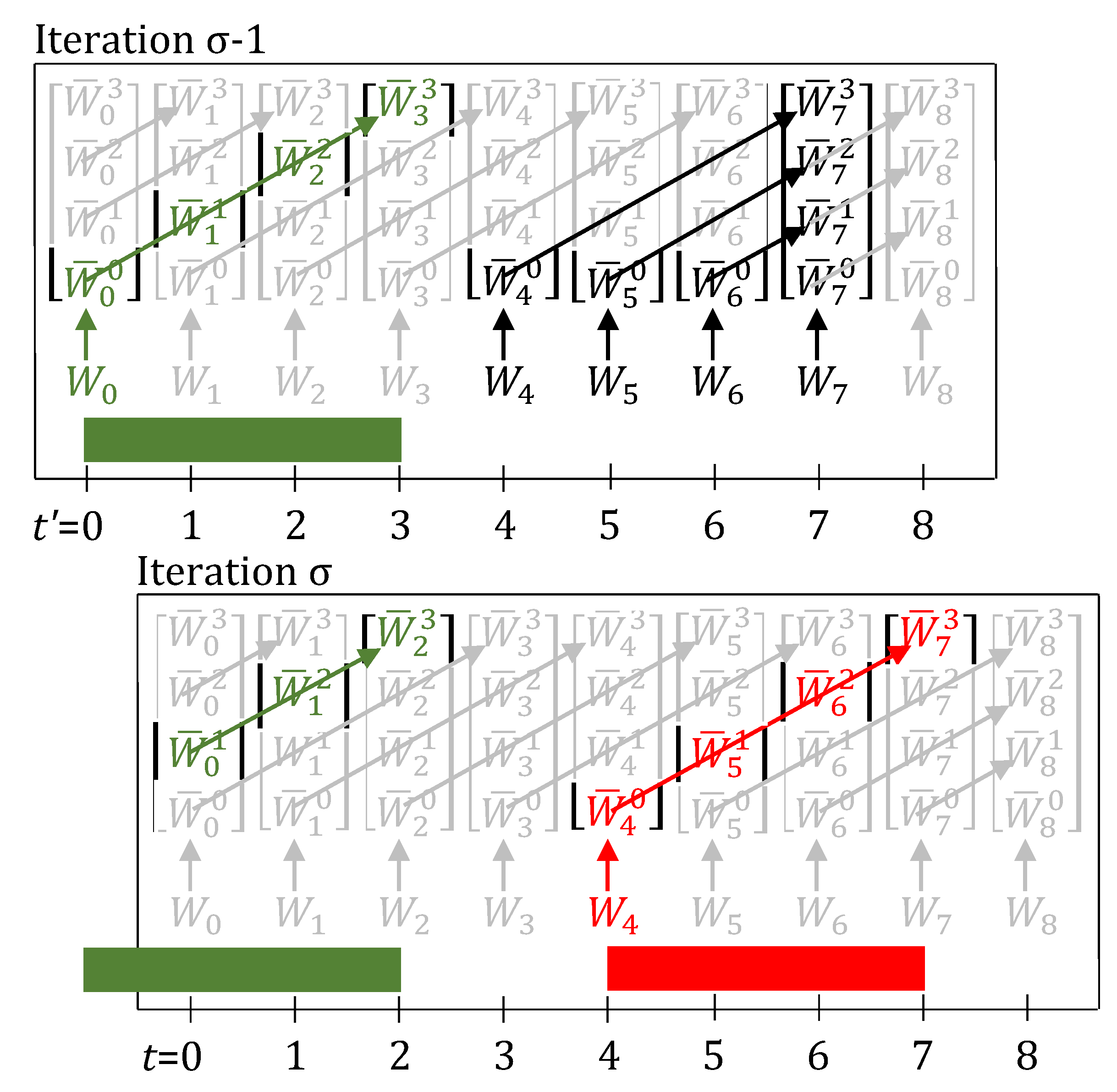
Figure 3.
When a 2 h delay is observed, through the lifting equations, evolve over the green trajectory, leading to the task correctly finishing 2 h late in iteration . Here, for the task is 3. Arrows show which variables are enforced as equal by the lifting equations (Equations (11) and (12), with delays present). Variables and parameters in green have a value of 1, rest have value 0. (A) The task now finishes at , instead of at . (B) The task now finishes at , instead of at . Through Equation (13), the unit is kept busy at and 1, by the inclusion of the terms and , and hence a new task is prevented from starting at these times. In addition, these terms in Equation (14), prevent the task’s produce from erroneously contributing to inventory ( and ).

Figure 4.
When a 2 h delay is observed, through the lifting equations, evolve over the green trajectory, leading to the task correctly finishing 2 h late in iteration . Here, for the task is 3. Arrows show which variables are enforced as equal by the lifting equations (Equations (22)–(24), with delays present). Variables and parameters in green have a value of 1, rest have value 0. (A) The task now finishes at , instead of at . Due to the update step, parameters , and variable are 1, hence, in iteration , due to the optimization model, , , and are also 1. (B) The task now finishes at , instead of at . The update step ensures that the true progress, n, of the task is reflected in the task-states at , i.e., .

Figure 5.
When a breakdown is observed, further evolution of the task-states for the task (the green trajectory), running on the unit that broke, stops. Here, for the task is 3 and the unit downtime (blue) is 2 h. Arrows show which variables are enforced as equal by the lifting equations (Equations (11) and (12), with breakdown present). Variables and parameters in green, blue, or red have a value of 1, rest have value 0. The green task is suspended at . A new task (red) can only start at , once the unit downtime is over. (A) Through Equation (13), the unit is kept busy at and 1, due to the terms and , respectively. (B) Through Equation (13), the unit is kept busy at and 1, due to the terms and , respectively. Additionally, the term in Equation (14), prevents the green task-state () from erroneously contributing to the inventory.

Figure 6.
When a breakdown is observed, further evolution of the task-states for the task (the green trajectory), running on the unit that broke, stops. Here, for the task is 3 and the unit downtime (blue) is 2 h. Arrows show which variables are enforced as equal by the lifting equations (Equations (22)–(24)). Variables and parameters in green, blue, or red have a value of 1, rest have value 0. The green task is suspended at . A new task (red) can only start at , once the unit downtime is over. Through Equation (25), the unit is kept busy at and 1, by the inclusion of the terms and . (A) The parameter , through Equation (20), prevents the task-state from evolving from to . (B) The parameter , through Equation (20), prevents the task-state from evolving from to .
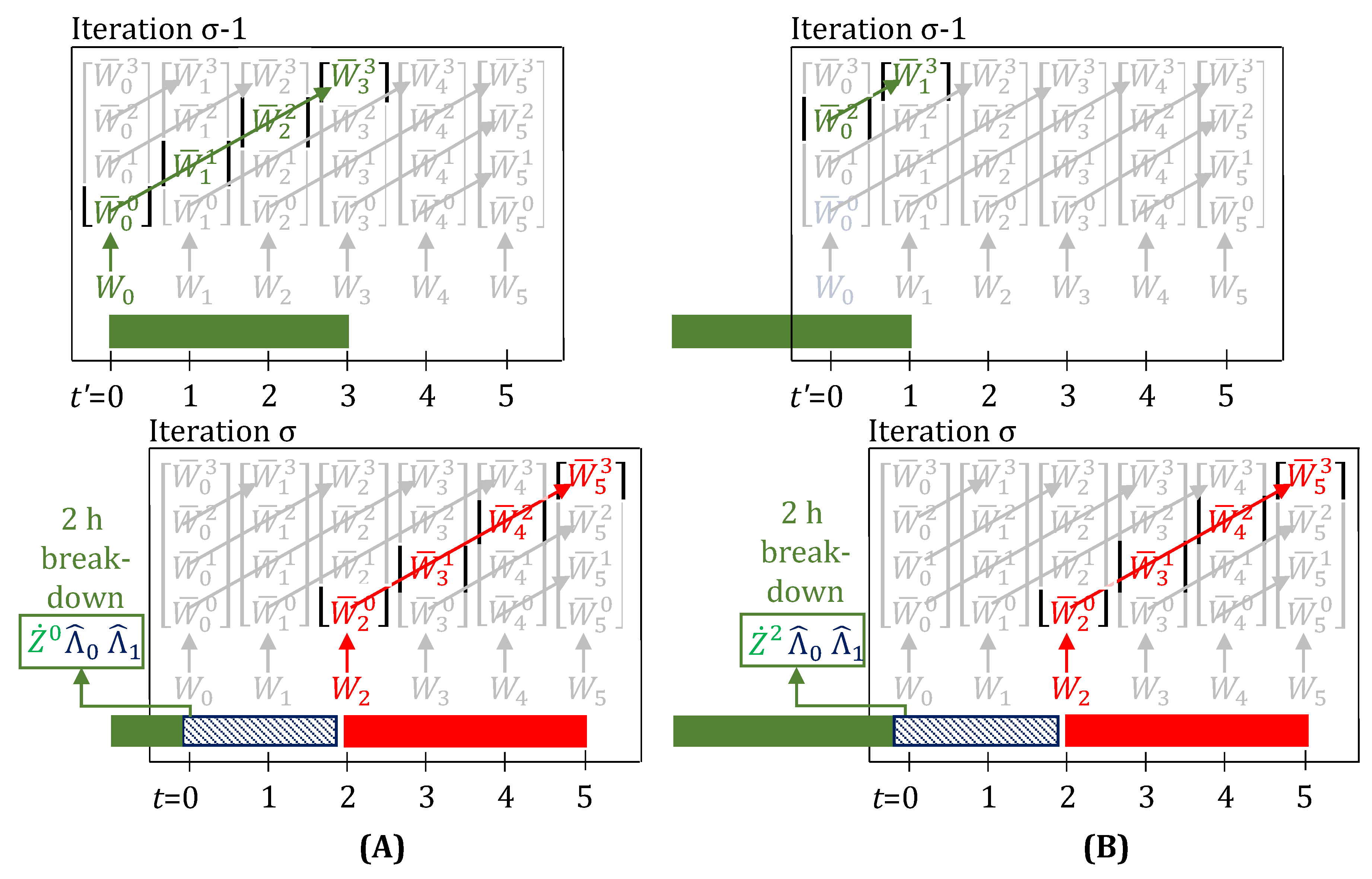
Figure 7.
The task has a nominal processing time . Time-grid spacing is h. Here, for ease of discussion, the time-grid is global, i.e., it is not reset for each iteration. (A) A delay (shown as oblique green pattern) of 0.66 h in time-period (0, 1) is observed. Since, , a delay of 1 h is applied at . This would ensure that the task finish is aligned with , even if the task actually ends at . The horizontal green pattern represents the fictitious extra task runtime to align with the discrete time-grid. Next, another delay of 0.2 h is observed in time-period (1, 2). Since, , no additional delay is applied in the update steps. This makes sense, because, the task finishes at in reality. Since, the previous delay was applied as 1 h, the task is now still thought to finish at , in alignment with the time-grid. Finally, when another delay of 0.66 h is observed in time-period (2, 3). Since, , a 1 h delay is applied in the update step. This correctly ensures that the task is now thought to end at , which is the round up of the true end time of h. (B) A break-down is observed at . Thus, for the update step between the iterations starting at and . If the downtime (blue) is 0.66 h, then the unit actually becomes available at . Thus, is not activated. This is indeed the case from our mathematical procedure as well, since, does not include any integer time-point. If h, then does span , and consequently . Finally, if h, then spans and , which results in and .

Figure 8.
In iteration , the green task () with a “large batch” is finishing at , but, due to the use of , is anticipated to produce only half of what the demand is. Thus, another identical green task is scheduled to start at , to satisfy the demand. With the use of , if the demand could be still be satisfied with a single “large” batch, a second batch wouldn’t be scheduled. In iteration , the earlier green task yields a large amount of material, in line with its large batch-size due to the true value of used at . (A) Since, here, there was no material handling loss, thus the second green task need not run now, as the demand was satisfied by the first batch itself. (B) Although the green task results in a large yield at , a small material handling loss () at , requires the second green task to still be scheduled in order to meet the demand, but now with a smaller batch-size. If there are no further material handling losses, there would be a small excess inventory of material produced by the second green task, since its batch-size was decided assuming the yield to be lower () but would in reality by higher ().
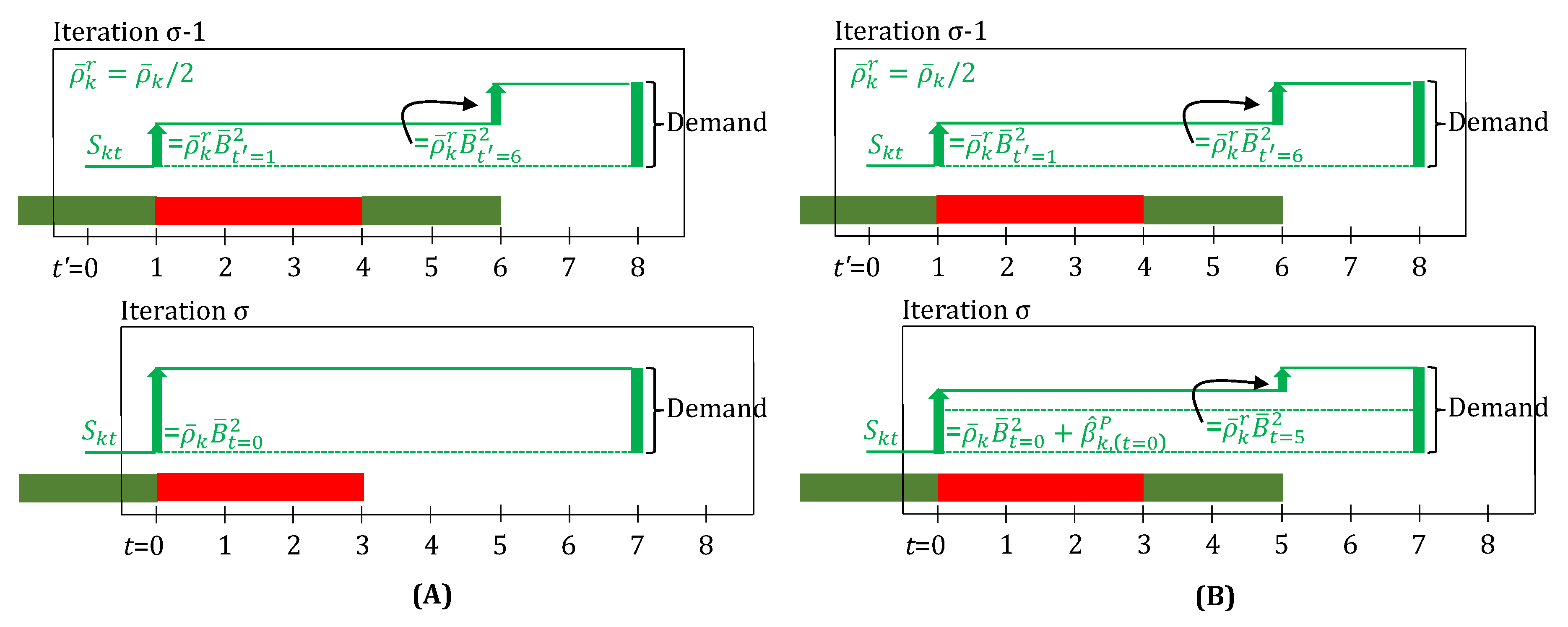
Figure 9.
For the green task (), a delay buffer of 1 h is chosen, i.e., . (A) In iteration , the model predicts that the green task will finish at . In the next iteration , when there is no delay in the green task, having run for 2 h, it correctly finishes at . No ad-hoc model changes are required in between the iterations to make this possible. Consequently, to take advantage of this nominal finish time of the green task, the red task, now starts 1 h earlier than what it was scheduled for in the previous iteration. (B) The green task, with conservative processing time, is scheduled to finish at in iteration . In iteration , a delay of 1 h is observed. The processing time delay buffer is maintained, and now the task is anticipated to finish at . In the next iteration (), the task correctly finishes at , accounting for the 1 h delay. The red task can now start on time at , or equivalently . Thus, having a delay buffer was useful, since it predicted a realistic start time for the red task in iteration itself.
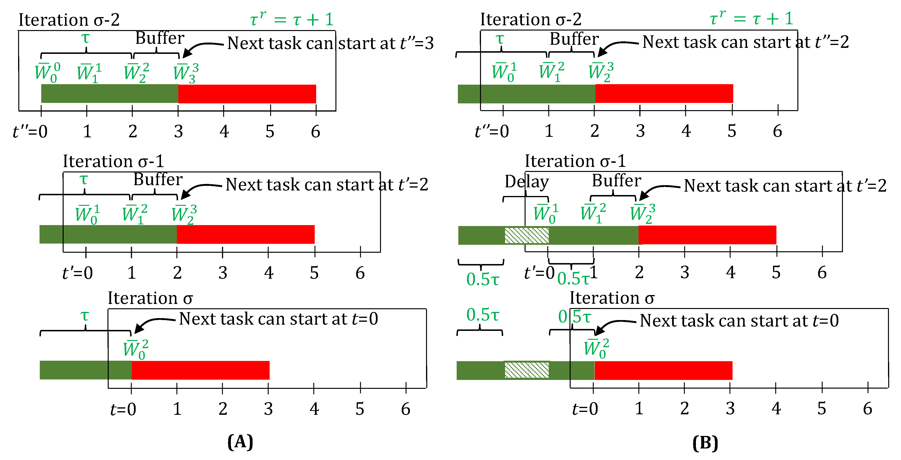
Figure 10.
Selected online scheduling iterations for the case study. The color of the tasks corresponds to their color in Figure 1. Executed schedule, with respect to each iteration, is shown in lighter (fainted) colors. The clock-time is the global time. Each iteration has its own local discrete time-grid.
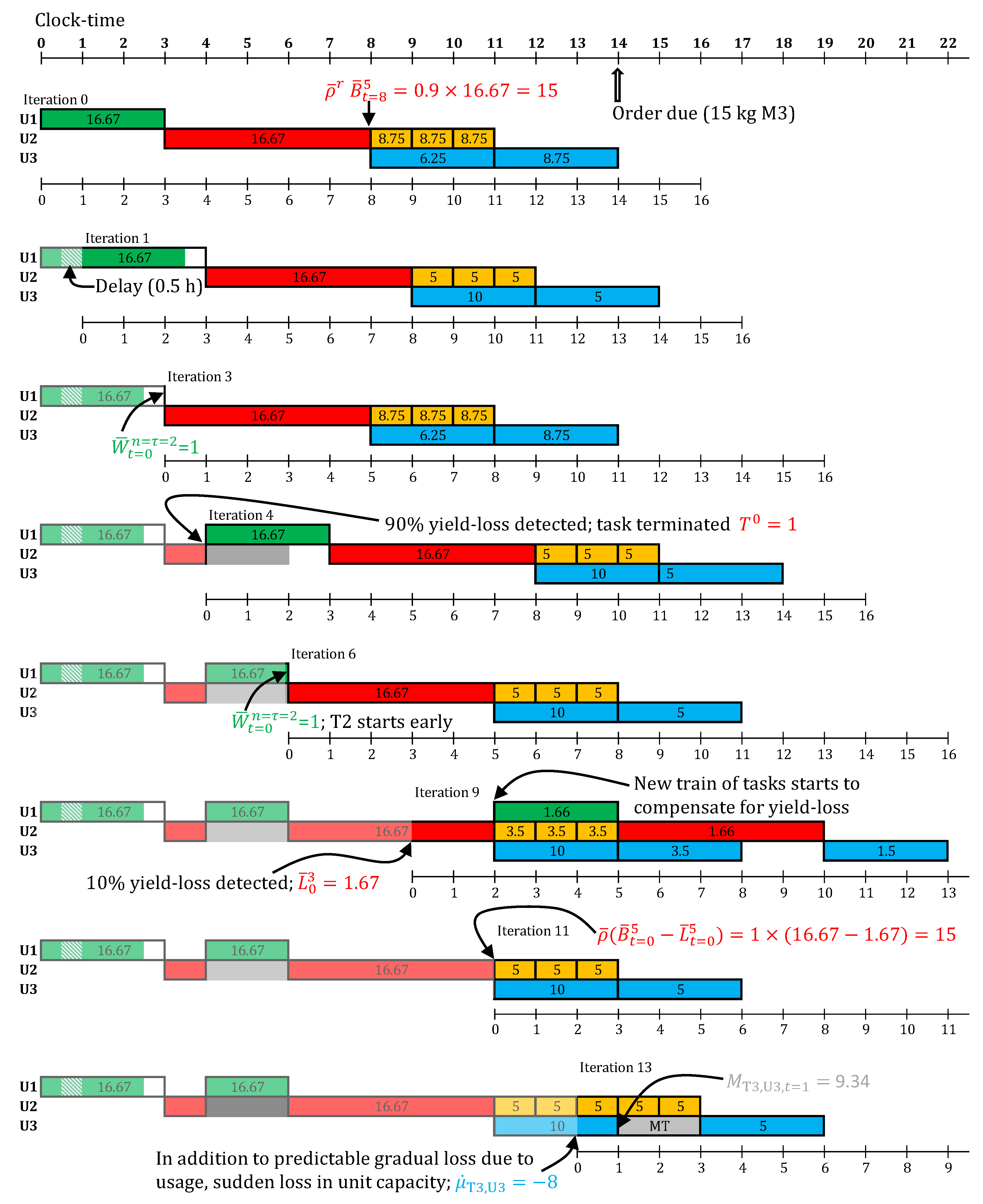

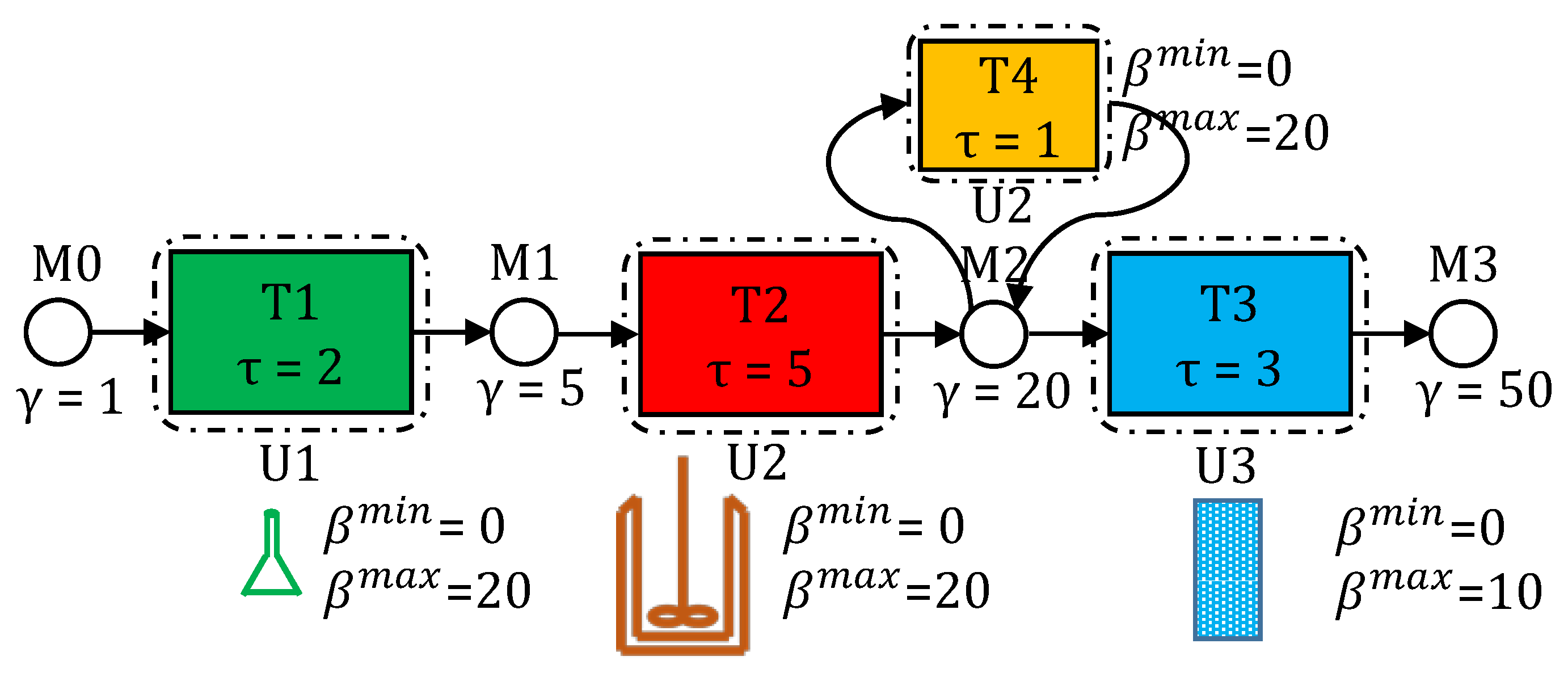
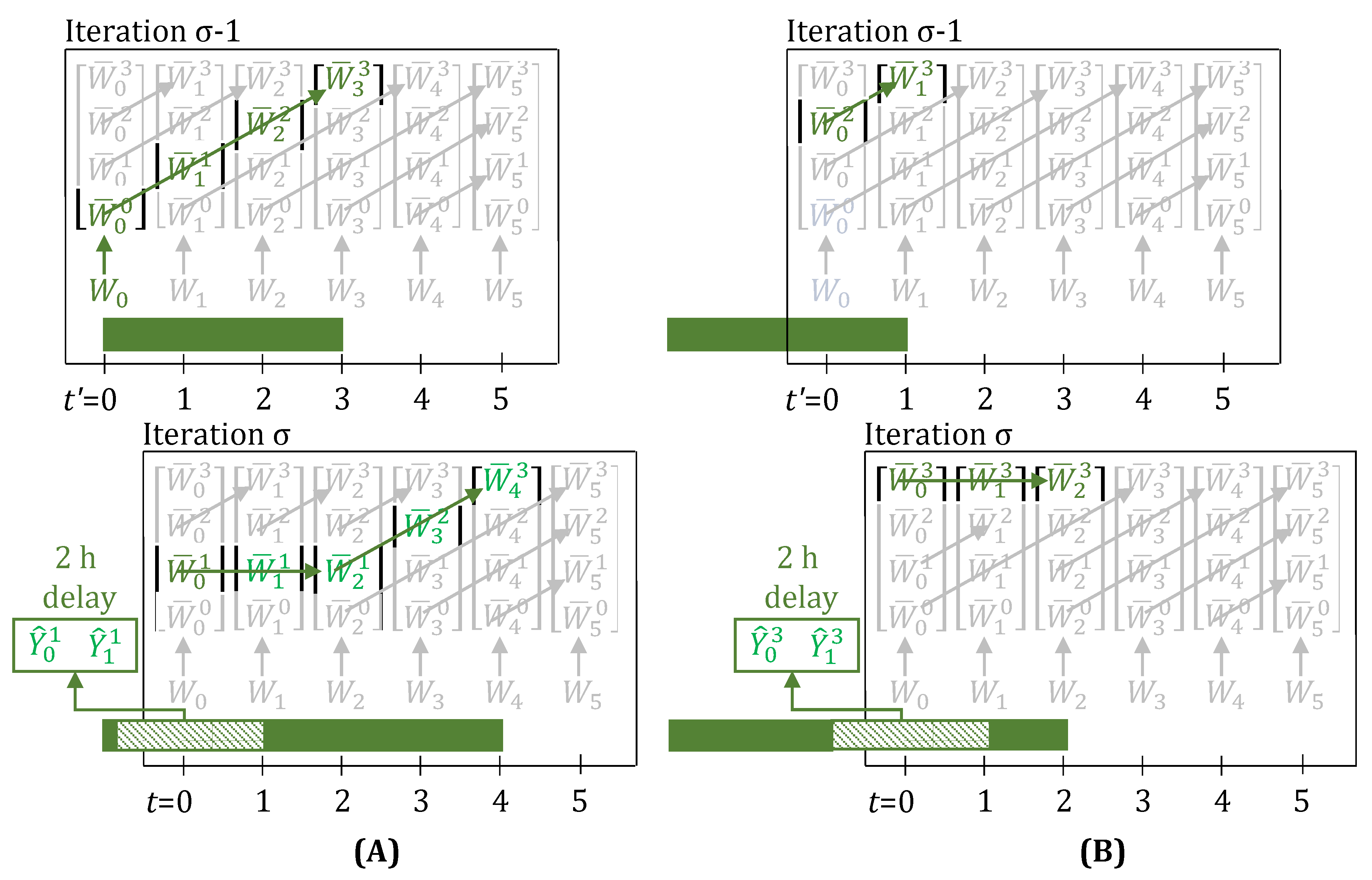
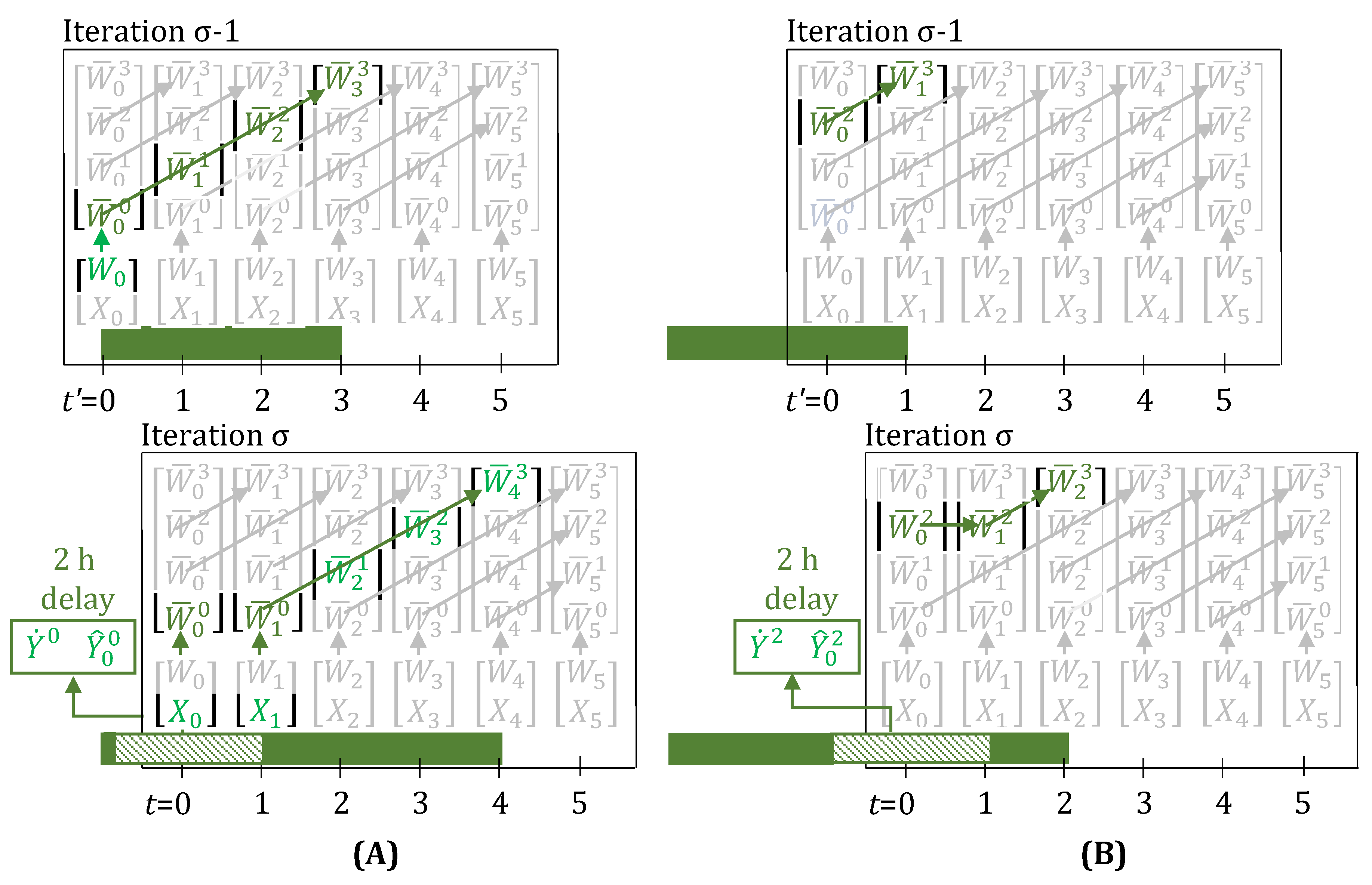
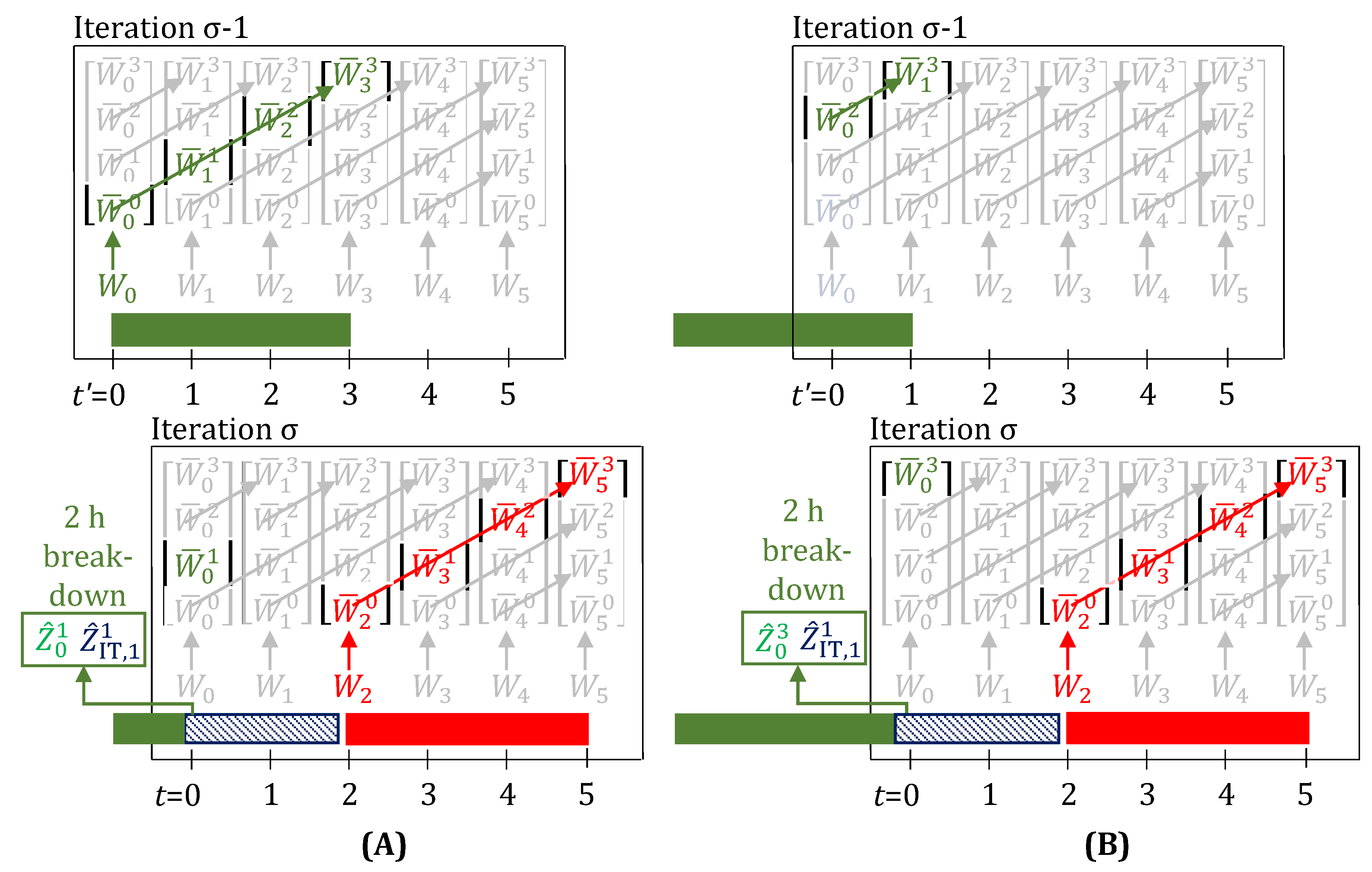
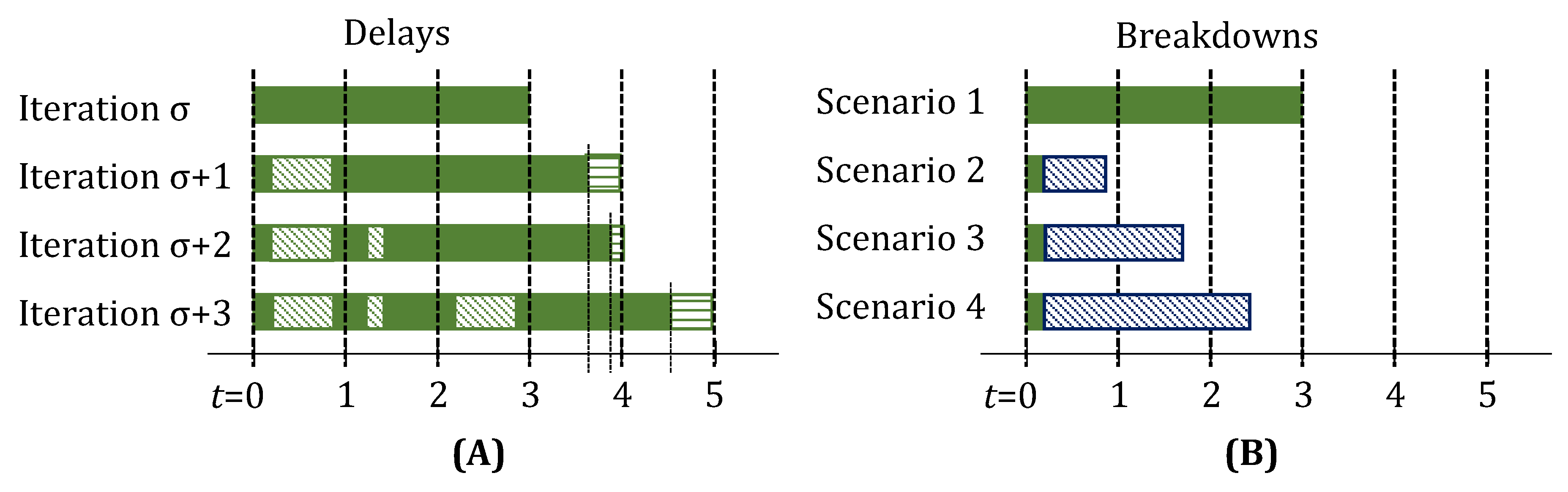
Table 1.
Parameter values for the case study.
© 2017 by the authors. Licensee MDPI, Basel, Switzerland. This article is an open access article distributed under the terms and conditions of the Creative Commons Attribution (CC BY) license (http://creativecommons.org/licenses/by/4.0/).
Share and Cite
MDPI and ACS Style
Gupta, D.; Maravelias, C.T. A General State-Space Formulation for Online Scheduling. Processes 2017, 5, 69. https://doi.org/10.3390/pr5040069
AMA Style
Gupta D, Maravelias CT. A General State-Space Formulation for Online Scheduling. Processes. 2017; 5(4):69. https://doi.org/10.3390/pr5040069
Chicago/Turabian StyleGupta, Dhruv, and Christos T. Maravelias. 2017. "A General State-Space Formulation for Online Scheduling" Processes 5, no. 4: 69. https://doi.org/10.3390/pr5040069
Note that from the first issue of 2016, this journal uses article numbers instead of page numbers. See further details here.