Economic Benefit from Progressive Integration of Scheduling and Control for Continuous Chemical Processes

 ,
, 
Abstract
:1. Introduction
1.1. Economic Benefit from Integrated Scheduling and Control
- (i)
- Rapid fluctuations in dynamic product demand;
- (ii)
- Rapid fluctuations in dynamic energy rates;
- (iii)
- Dynamic production costs;
- (iv)
- Benefits of increased energy efficiency;
- (v)
- Necessity of control-level dynamics information for optimal production schedule calculation.
1.2. Previous Work
1.2.1. Integrating Process Dynamics into Scheduling
1.2.2. Reactive Integrated Scheduling and Control
1.2.3. Responsiveness to Market Fluctuations
1.3. Purpose of This Work
2. Phases of Progressive Integration
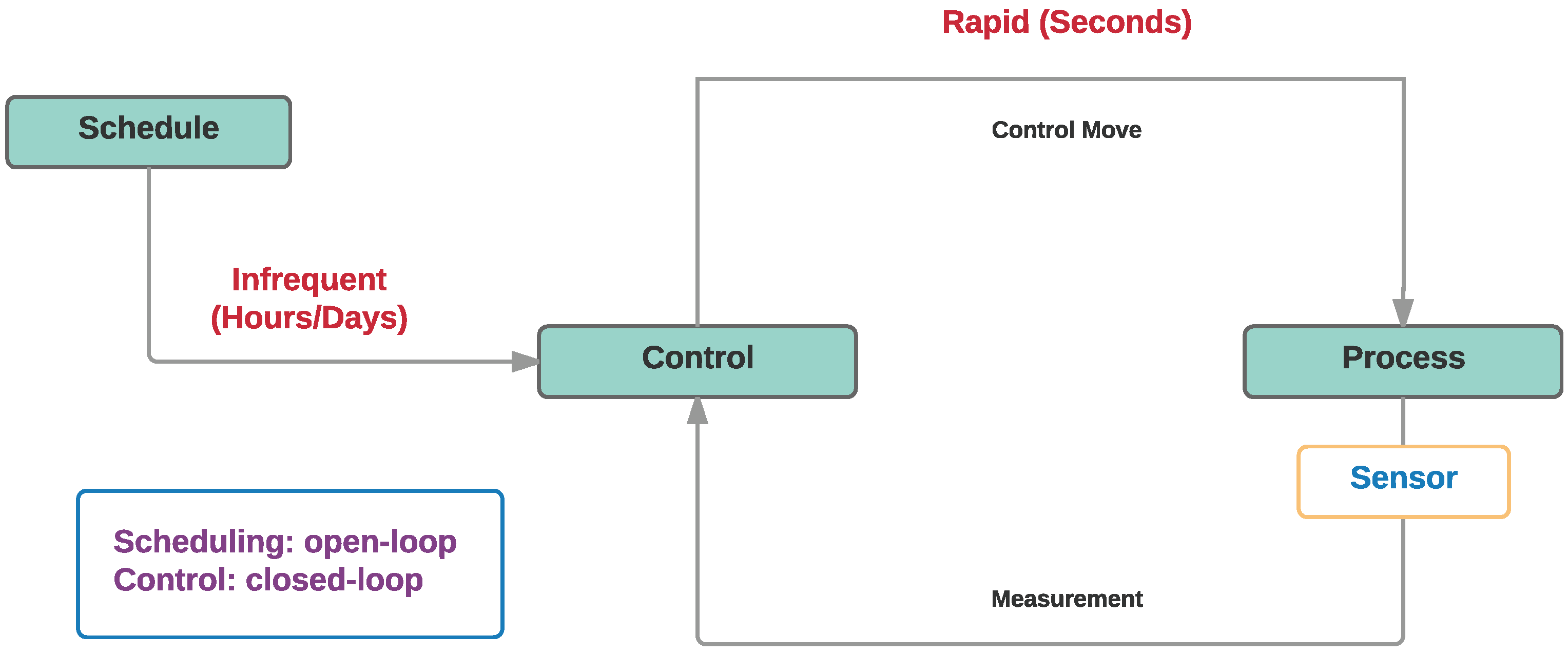
2.1. Phase 1: Fully Segregated Scheduling and Control
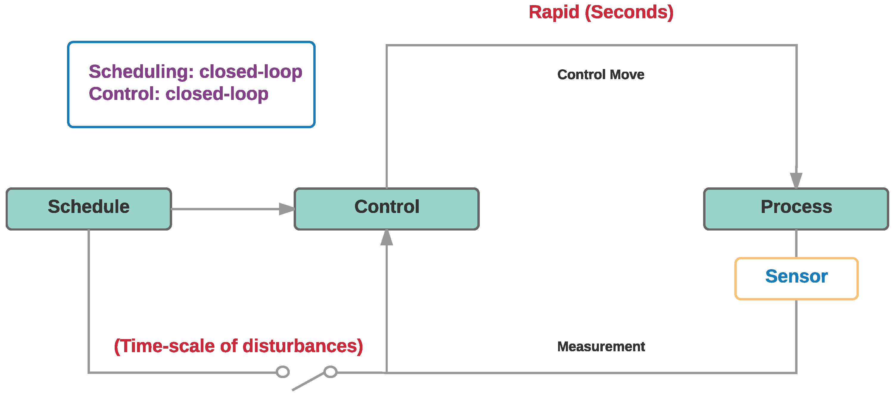
2.2. Phase 2: Reactive Closed-Loop Segregated Scheduling and Control
2.3. Phase 3: Open-Loop Integrated Scheduling and Control
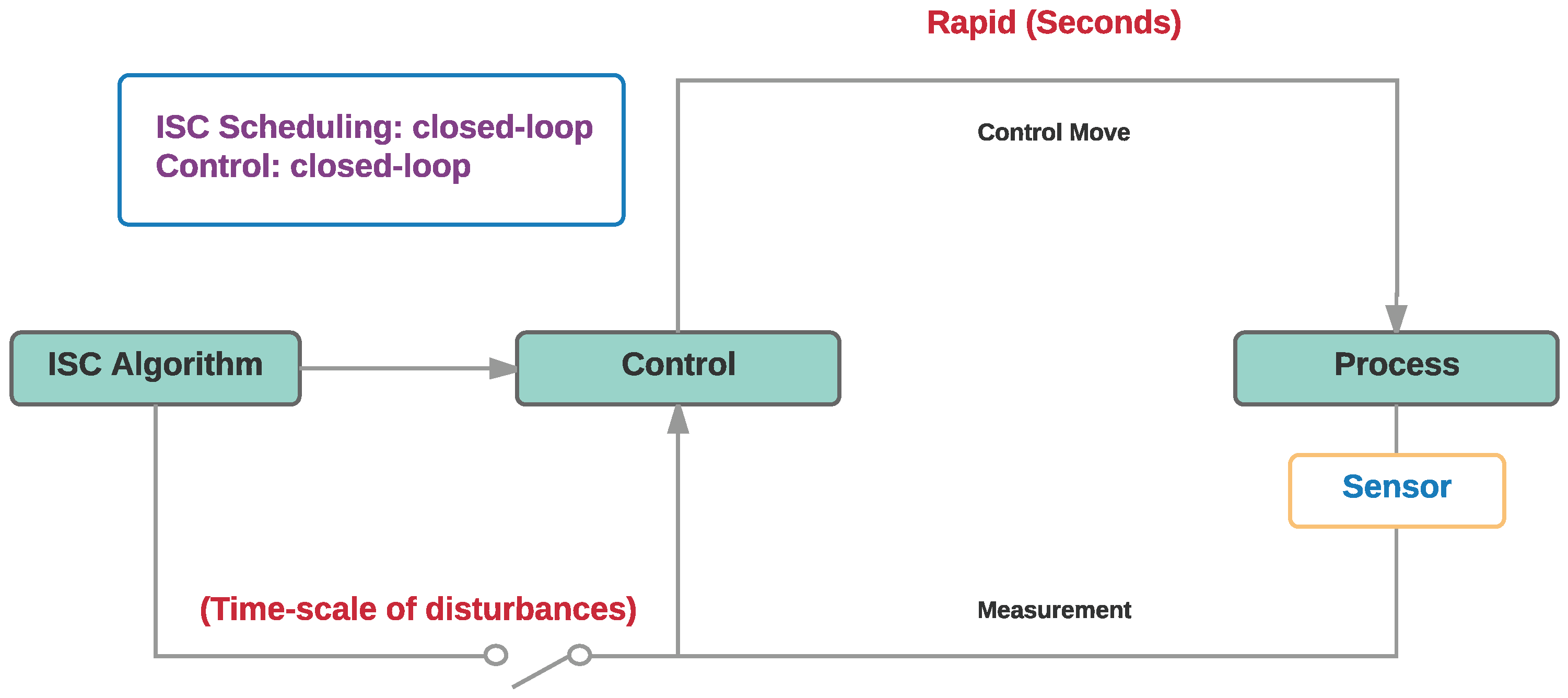
2.4. Phase 4: Closed-Loop Integrated Scheduling and Control Responsive to Market Fluctuations
2.5. Mathematical Formulation
3. Case Study Application
3.1. Process Model
- Constant volume;
- Well mixed;
- Constant density.
3.2. Scenarios
- (A)
- Process disturbance ;
- (B)
- Demand disturbance;
- (C)
- Price disturbance.
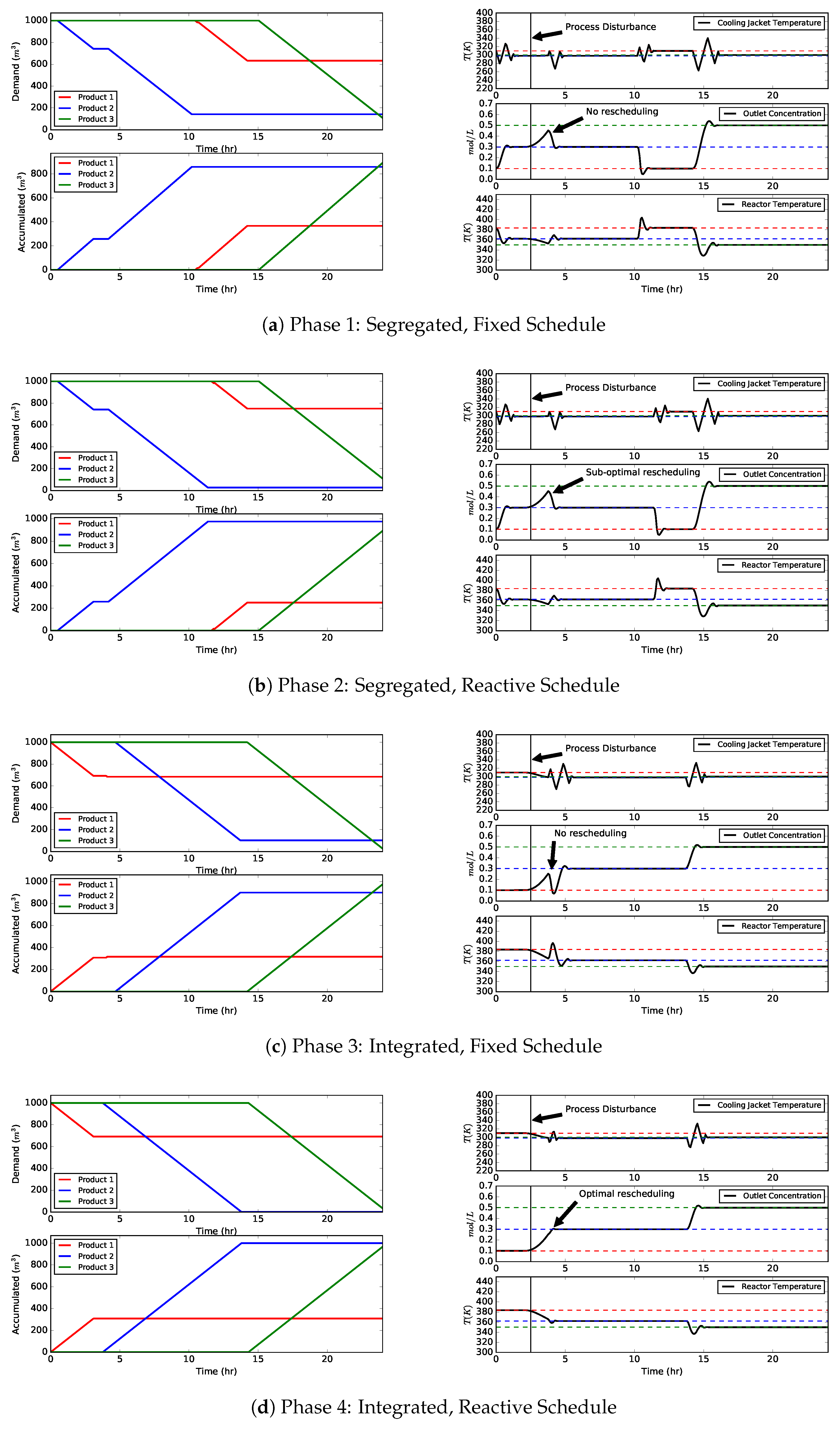
4. Results
4.1. Scenario A: Process Disturbance
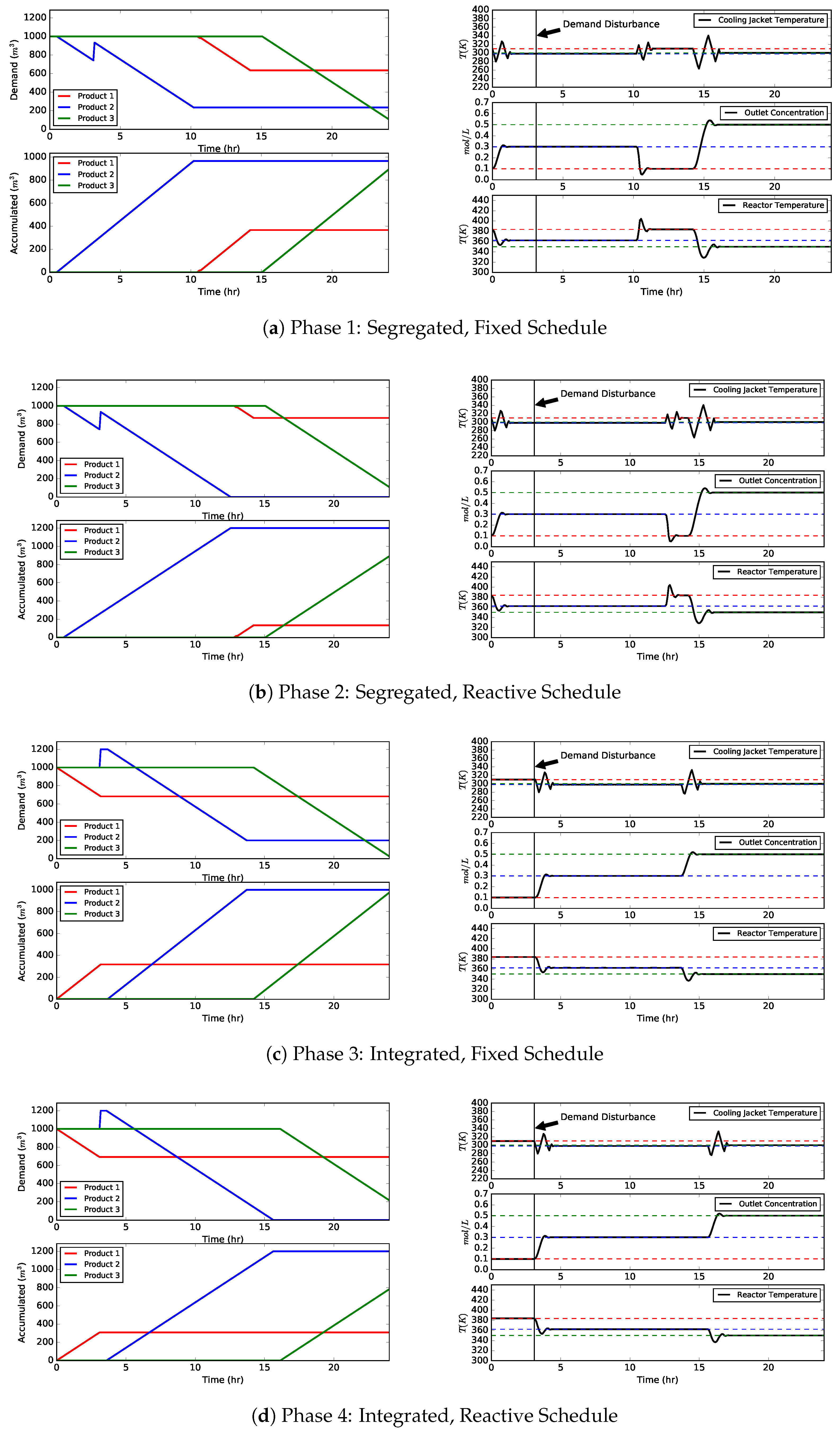
4.2. Scenario B: Market Update Containing Demand Fluctuation
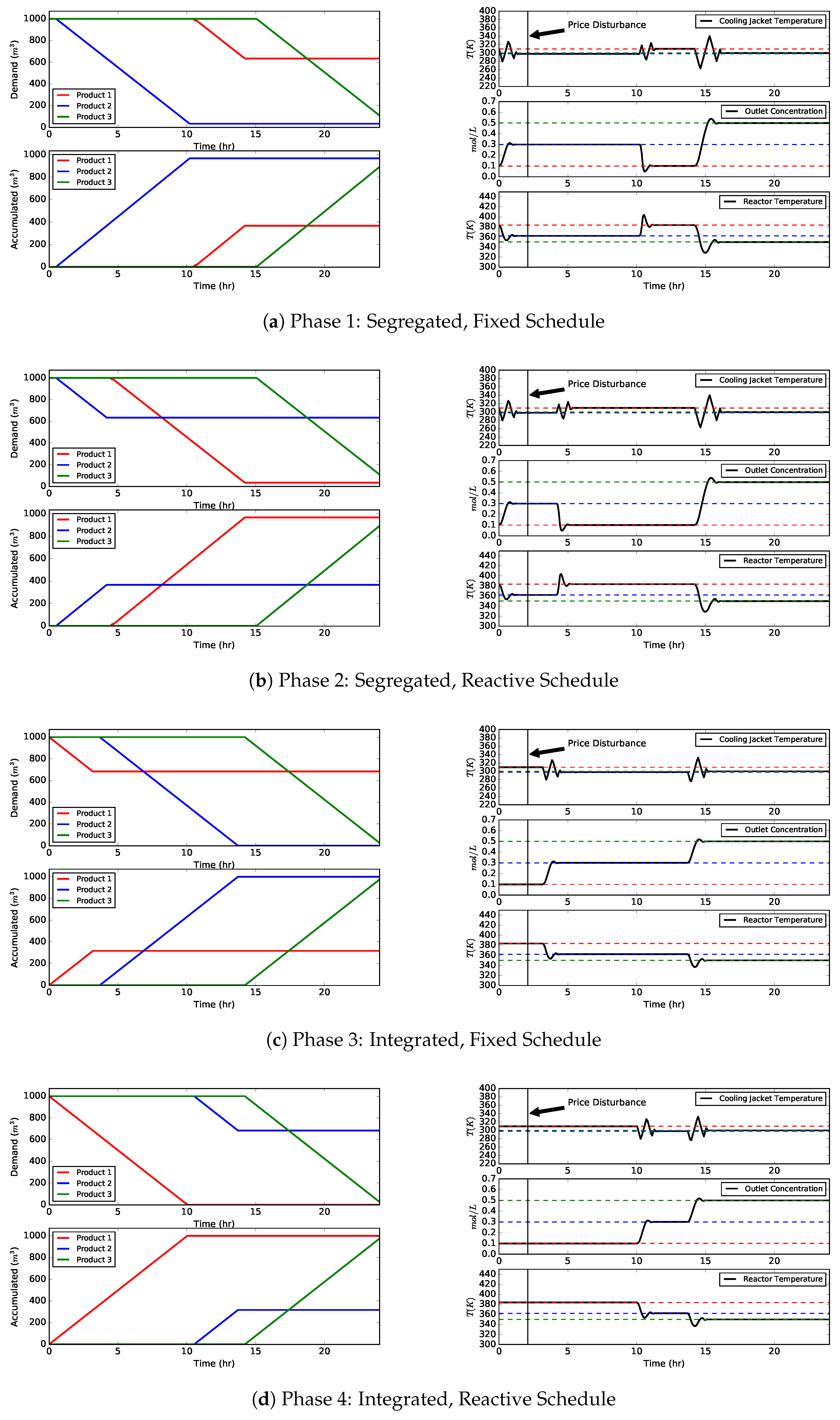
4.3. Scenario C: Market Update Containing New Product Selling Prices
5. Conclusions
Directions for Future Work
Acknowledgments
Author Contributions
Conflicts of Interest
Abbreviations
| ISC | integrated scheduling and control |
| SSC | segregated scheduling and control |
| MINLP | mixed-integer nonlinear programming |
| NLP | nonlinear programming |
| CSTR | continuous stirred tank reactor |
| MIDO | mixed-integer dynamic optimization |
| MILP | mixed-integer linear programming |
| NMPC | nonlinear model predictive control |
| ASU | air separation unit |
| MMA | methyl methacrylate reactor |
| FBR | fluidized bed reactor |
| RTN | resource task network |
| HIPS | high impact polystyrene reactor |
| ASU | cryogenic air separation unit |
| SISO | single-input single-output |
| PFR | plug flow reactor |
| PWA | piecewise affine |
| DR | demand response |
References
- Backx, T.; Bosgra, O.; Marquardt, W. Integration of Model Predictive Control and Optimization of Processes. In Proceedings of the ADCHEM 2000 International Symposium on Advanced Control of Chemical Processes, Pisa, Italy, 14–16 June 2000; pp. 249–260. [Google Scholar]
- Soderstrom, T.A.; Zhan, Y.; Hedengren, J. Advanced Process Control in ExxonMobil Chemical Company: Successes and Challenges. In Proceedings of the AIChE Spring Meeting, Salt Lake City, UT, USA, 7–12 Novembrer 2010; pp. 1–12. [Google Scholar]
- Baldea, M.; Harjunkoski, I. Integrated production scheduling and process control: A systematic review. Comput. Chem. Eng. 2014, 71, 377–390. [Google Scholar] [CrossRef]
- Nyström, R.H.; Harjunkoski, I.; Kroll, A. Production optimization for continuously operated processes with optimal operation and scheduling of multiple units. Comput. Chem. Eng. 2006, 30, 392–406. [Google Scholar] [CrossRef]
- Chatzidoukas, C.; Perkins, J.D.; Pistikopoulos, E.N.; Kiparissides, C. Optimal grade transition and selection of closed-loop controllers in a gas-phase olefin polymerization fluidized bed reactor. Chem. Eng. Sci. 2003, 58, 3643–3658. [Google Scholar] [CrossRef]
- Capón-García, E.; Guillén-Gosálbez, G.; Espuña, A. Integrating process dynamics within batch process scheduling via mixed-integer dynamic optimization. Chem. Eng. Sci. 2013, 102, 139–150. [Google Scholar] [CrossRef]
- Nie, Y.; Biegler, L.T.; Wassick, J.M. Integrated scheduling and dynamic optimization of batch processes using state equipment networks. AIChE J. 2012, 58, 3416–3432. [Google Scholar] [CrossRef]
- Flores-Tlacuahuac, A.; Grossmann, I.E. Simultaneous scheduling and control of multiproduct continuous parallel lines. Ind. Eng. Chem. Res. 2010, 49, 7909–7921. [Google Scholar] [CrossRef]
- Terrazas-Moreno, S.; Flores-Tlacuahuac, A.; Grossmann, I.E. Lagrangean heuristic for the scheduling and control of polymerization reactors. AIChE J. 2008, 54, 163–182. [Google Scholar] [CrossRef]
- Pattison, R.C.; Touretzky, C.R.; Harjunkoski, I.; Baldea, M. Moving Horizon Closed-Loop Production Scheduling Using Dynamic Process Models. AIChE J. 2017, 63, 639–651. [Google Scholar] [CrossRef]
- Engell, S.; Harjunkoski, I. Optimal operation: Scheduling, advanced control and their integration. Comput. Chem. Eng. 2012, 47, 121–133. [Google Scholar] [CrossRef]
- Harjunkoski, I.; Maravelias, C.T.; Bongers, P.; Castro, P.M.; Engell, S.; Grossmann, I.E.; Hooker, J.; Méndez, C.; Sand, G.; Wassick, J. Scope for industrial applications of production scheduling models and solution methods. Comput. Chem. Eng. 2014, 62, 161–193. [Google Scholar] [CrossRef]
- Harjunkoski, I.; Nyström, R.; Horch, A. Integration of scheduling and control—Theory or practice? Comput. Chem. Eng. 2009, 33, 1909–1918. [Google Scholar] [CrossRef]
- Shobrys, D.E.; White, D.C. Planning, scheduling and control systems: Why cannot they work together. Comput. Chem. Eng. 2002, 26, 149–160. [Google Scholar] [CrossRef]
- Baldea, M.; Du, J.; Park, J.; Harjunkoski, I. Integrated production scheduling and model predictive control of continuous processes. AIChE J. 2015, 61, 4179–4190. [Google Scholar] [CrossRef]
- Baldea, M.; Touretzky, C.R.; Park, J.; Pattison, R.C. Handling Input Dynamics in Integrated Scheduling and Control. In Proceedings of the 2016 IEEE International Conference on Automation, Quality and Testing, Robotics (AQTR), Cluj-Napoca, Romania, 19–21 May 2016; pp. 1–6. [Google Scholar]
- Baldea, M. Employing Chemical Processes as Grid-Level Energy Storage Devices. Adv. Energy Syst. Eng. 2017, 247–271. [Google Scholar] [CrossRef]
- Beal, L.D.R.; Clark, J.D.; Anderson, M.K.; Warnick, S.; Hedengren, J.D. Combined Scheduling and Control with Diurnal Constraints and Costs Using a Discrete Time Formulation. In Proceedings of the FOCAPO/CPC, Tucson, Arizona, 8–12 January 2017. [Google Scholar]
- Beal, L.D.; Petersen, D.; Grimsman, D.; Warnick, S.; Hedengren, J.D. Integrated Scheduling and Control in Discrete-Time with Dynamic Parameters and Constraints. Comput. Chem. Eng. 2008, 32, 463–476. [Google Scholar]
- Beal, L.D.; Park, J.; Petersen, D.; Warnick, S.; Hedengren, J.D. Combined model predictive control and scheduling with dominant time constant compensation. Comput. Chem. Eng. 2017, 104, 271–282. [Google Scholar] [CrossRef]
- Cai, Y.; Kutanoglu, E.; Hasenbein, J.; Qin, J. Single-machine scheduling with advanced process control constraints. J. Sched. 2012, 15, 165–179. [Google Scholar] [CrossRef]
- Chatzidoukas, C.; Kiparissides, C.; Perkins, J.D.; Pistikopoulos, E.N. Optimal grade transition campaign scheduling in a gas-phase polyolefin FBR using mixed integer dynamic optimization. Comput. Aided Chem. Eng. 2003, 15, 744–747. [Google Scholar]
- Chatzidoukas, C.; Pistikopoulos, S.; Kiparissides, C. A Hierarchical Optimization Approach to Optimal Production Scheduling in an Industrial Continuous Olefin Polymerization Reactor. Macromol. React. Eng. 2009, 3, 36–46. [Google Scholar] [CrossRef]
- Chu, Y.; You, F. Integration of scheduling and control with online closed-loop implementation: Fast computational strategy and large-scale global optimization algorithm. Comput. Chem. Eng. 2012, 47, 248–268. [Google Scholar] [CrossRef]
- Chu, Y.; You, F. Integration of production scheduling and dynamic optimization for multi-product CSTRs: Generalized Benders decomposition coupled with global mixed-integer fractional programming. Comput. Chem. Eng. 2013, 58, 315–333. [Google Scholar] [CrossRef]
- Chu, Y.; You, F. Integrated Scheduling and Dynamic Optimization of Sequential Batch Proesses with Online Implementation. AIChE J. 2013, 59, 2379–2406. [Google Scholar] [CrossRef]
- Chu, Y.; You, F. Integrated Scheduling and Dynamic Optimization of Complex Batch Processes with General Network Structure Using a Generalized Benders Decomposition Approach. Ind. Eng. Chem. Res. 2013, 52, 7867–7885. [Google Scholar] [CrossRef]
- Chu, Y.; You, F. Integration of scheduling and dynamic optimization of batch processes under uncertainty: Two-stage stochastic programming approach and enhanced generalized benders decomposition algorithm. Ind. Eng. Chem. Res. 2013, 52, 16851–16869. [Google Scholar] [CrossRef]
- Chu, Y.; You, F. Moving Horizon Approach of Integrating Scheduling and Control for Sequential Batch Processes. AIChE J. 2014, 60, 1654–1671. [Google Scholar] [CrossRef]
- Chu, Y.; You, F. Integrated Planning, Scheduling, and Dynamic Optimization for Batch Processes: MINLP Model Formulation and Efficient Solution Methods via Surrogate Modeling. Ind. Eng. Chem. Res. 2014, 53, 13391–13411. [Google Scholar] [CrossRef]
- Chu, Y.; You, F. Integrated scheduling and dynamic optimization by stackelberg game: Bilevel model formulation and efficient solution algorithm. Ind. Eng. Chem. Res. 2014, 53, 5564–5581. [Google Scholar] [CrossRef]
- Dias, L.S.; Ierapetritou, M.G. Integration of scheduling and control under uncertainties: Review and challenges. Chem. Eng. Res. Des. 2016, 116, 98–113. [Google Scholar] [CrossRef]
- Du, J.; Park, J.; Harjunkoski, I.; Baldea, M. A time scale-bridging approach for integrating production scheduling and process control. Comput. Chem. Eng. 2015, 79, 59–69. [Google Scholar] [CrossRef]
- Flores-Tlacuahuac, A.; Grossmann, I.E. Simultaneous Cyclic Scheduling and Control of a Multiproduct CSTR. Ind. Eng. Chem. Res. 2006, 45, 6698–6712. [Google Scholar] [CrossRef]
- Gutierrez-Limon, M.A.; Flores-Tlacuahuac, A.; Grossmann, I.E. A Multiobjective Optimization Approach for the Simultaneous Single Line Scheduling and Control of CSTRs. Ind. Eng. Chem. Res. 2011, 51, 5881–5890. [Google Scholar] [CrossRef]
- Gutierrez-Limon, M.A.; Flores-Tlacuahuac, A.; Grossmann, I.E. A reactive optimization strategy for the simultaneous planning, scheduling and control of short-period continuous reactors. Comput. Chem. Eng. 2016, 84, 507–515. [Google Scholar] [CrossRef]
- Gutiérrez-Limón, M.A.; Flores-Tlacuahuac, A.; Grossmann, I.E. MINLP formulation for simultaneous planning, scheduling, and control of short-period single-unit processing systems. Ind. Eng. Chem. Res. 2014, 53, 14679–14694. [Google Scholar] [CrossRef]
- Koller, R.W.; Ricardez-Sandoval, L.A. A Dynamic Optimization Framework for Integration of Design, Control and Scheduling of Multi-product Chemical Processes under Disturbance and Uncertainty. Comput. Chem. Eng. 2017, 106, 147–159. [Google Scholar] [CrossRef]
- Nie, Y.; Biegler, L.T.; Villa, C.M.; Wassick, J.M. Discrete Time Formulation for the Integration of Scheduling and Dynamic Optimization. Ind. Eng. Chem. Res. 2015, 54, 4303–4315. [Google Scholar] [CrossRef]
- Nyström, R.H.; Franke, R.; Harjunkoski, I.; Kroll, A. Production campaign planning including grade transition sequencing and dynamic optimization. Comput. Chem. Eng. 2005, 29, 2163–2179. [Google Scholar] [CrossRef]
- Patil, B.P.; Maia, E.; Ricardez-Sandoval, L.A. Integration of Scheduling, Design, and Control of Multiproduct Chemical Processes Under Uncertainty. AIChE J. 2015, 61, 2456–2470. [Google Scholar] [CrossRef]
- Pattison, R.C.; Touretzky, C.R.; Johansson, T.; Harjunkoski, I.; Baldea, M. Optimal Process Operations in Fast-Changing Electricity Markets: Framework for Scheduling with Low-Order Dynamic Models and an Air Separation Application. Ind. Eng. Chem. Res. 2016, 55, 4562–4584. [Google Scholar] [CrossRef]
- Prata, A.; Oldenburg, J.; Kroll, A.; Marquardt, W. Integrated scheduling and dynamic optimization of grade transitions for a continuous polymerization reactor. Comput. Chem. Eng. 2008, 32, 463–476. [Google Scholar] [CrossRef]
- Terrazas-Moreno, S.; Flores-Tlacuahuac, A.; Grossmann, I.E. Simultaneous design, scheduling, and optimal control of a methyl-methacrylate continuous polymerization reactor. AIChE J. 2008, 54, 3160–3170. [Google Scholar] [CrossRef]
- Terrazas-Moreno, S.; Flores-Tlacuahuac, A.; Grossmann, I.E. Simultaneous cyclic scheduling and optimal control of polymerization reactors. AIChE J. 2007, 53, 2301–2315. [Google Scholar] [CrossRef]
- You, F.; Grossmann, I.E. Design of responsive supply chains under demand uncertainty. Comput. Chem. Eng. 2008, 32, 3090–3111. [Google Scholar] [CrossRef]
- Zhuge, J.; Ierapetritou, M.G. Integration of Scheduling and Control with Closed Loop Implementation. Ind. Eng. Chem. Res. 2012, 51, 8550–8565. [Google Scholar] [CrossRef]
- Zhuge, J.; Ierapetritou, M.G. Integration of Scheduling and Control for Batch Processes Using Multi-Parametric Model Predictive Control. AIChE J. 2014, 60, 3169–3183. [Google Scholar] [CrossRef]
- Zhuge, J.; Ierapetritou, M.G. An Integrated Framework for Scheduling and Control Using Fast Model Predictive Control. AIChE J. 2015, 61, 3304–3319. [Google Scholar] [CrossRef]
- Zhuge, J.; Ierapetritou, M.G. A Decomposition Approach for the Solution of Scheduling Including Process Dynamics of Continuous Processes. Ind. Eng. Chem. Res. 2016, 55, 1266–1280. [Google Scholar] [CrossRef]
- Mahadevan, R.; Doyle, F.J.; Allcock, A.C. Control-relevant scheduling of polymer grade transitions. AIChE J. 2002, 48, 1754–1764. [Google Scholar] [CrossRef]
- Mojica, J.L.; Petersen, D.; Hansen, B.; Powell, K.M.; Hedengren, J.D. Optimal combined long-term facility design and short-term operational strategy for CHP capacity investments. Energy 2017, 118, 97–115. [Google Scholar] [CrossRef]
- Gupta, D.; Maravelias, C.T.; Wassick, J.M. From rescheduling to online scheduling. Chem. Eng. Res. Des. 2016, 116, 83–97. [Google Scholar] [CrossRef]
- Gupta, D.; Maravelias, C.T. On deterministic online scheduling: Major considerations, paradoxes and remedies. Comput. Chem. Eng. 2016, 94, 312–330. [Google Scholar] [CrossRef]
- Gupta, D.; Maravelias, C.T. A General State-Space Formulation for Online Scheduling. Processes 2017, 4, 69. [Google Scholar] [CrossRef]
- Kopanos, G.M.; Pistikopoulos, E.N. Reactive scheduling by a multiparametric programming rolling horizon framework: A case of a network of combined heat and power units. Ind. Eng. Chem. Res. 2014, 53, 4366–4386. [Google Scholar] [CrossRef]
- Liu, S.; Shah, N.; Papageorgiou, L.G. Multiechelon Supply Chain Planning With Sequence-Dependent Changeovers and Price Elasticity of Demand under Uncertainty. AIChE J. 2012, 58, 3390–3403. [Google Scholar] [CrossRef]
- Touretzky, C.R.; Baldea, M. Integrating scheduling and control for economic MPC of buildings with energy storage. J. Process Control 2014, 24, 1292–1300. [Google Scholar] [CrossRef]
- Li, Z.; Ierapetritou, M.G. Process Scheduling Under Uncertainty Using Multiparametric Programming. AIChE J. 2007, 53, 3183–3203. [Google Scholar] [CrossRef]
- Petersen, D.; Beal, L.D.R.; Prestwich, D.; Warnick, S.; Hedengren, J.D. Combined Noncyclic Scheduling and Advanced Control for Continuous Chemical Processes. Processes 2017, 4, 83. [Google Scholar] [CrossRef]
- Hart, W.E.; Watson, J.P.; Woodruff, D.L. Pyomo: Modeling and solving mathematical programs in Python. Math. Program. Comput. 2011, 3, 219–260. [Google Scholar] [CrossRef]
- Hart, W.E.; Laird, C.; Watson, J.P.; Woodruff, D.L. Pyomo—Optimization Modeling in Python; Springer Science+Business Media, LLC: Berlin/Heidelberg, Germany, 2012; Volume 67. [Google Scholar]
- Carey, G.; Finlayson, B.A. Orthogonal collocation on finite elements for elliptic equations. Chem. Eng. Sci. 1975, 30, 587–596. [Google Scholar] [CrossRef]
- Hedengren, J.; Mojica, J.; Cole, W.; Edgar, T. APOPT: MINLP Solver for Differential Algebraic Systems with Benchmark Testing. In Proceedings of the INFORMS Annual Meeting, Pheonix, AZ, USA, 14–17 October 2012. [Google Scholar]
- Belotti, P.; Lee, J.; Liberti, L.; Margot, F.; Wächter, A. Branching and bounds tightening techniques for non-convex MINLP. Optim. Methods Softw. 2009, 24, 597–634. [Google Scholar] [CrossRef]
- Floudas, C.A.; Lin, X. Continuous-time versus discrete-time approaches for scheduling of chemical processes: A review. Comput. Chem. Eng. 2004, 28, 2109–2129. [Google Scholar] [CrossRef]
- Sundaramoorthy, A.; Maravelias, C.T. Computational study of network-based mixed-integer programming approaches for chemical production scheduling. Ind. Eng. Chem. Res. 2011, 50, 5023–5040. [Google Scholar] [CrossRef]


| Author | Shows Benefit of ISC over SSC | Batch Process | Continuous Process | Example Application (s) |
|---|---|---|---|---|
| Baldea et al. (2015) [15] | X | CSTR | ||
| Baldea et al. (2016) [16] | X | MMA | ||
| Baldea (2017) [17] | X | DR chemical processes and power generation facilities | ||
| Beal (2017) [18] | X | CSTR | ||
| Beal (2017) [19] | X | CSTR | ||
| Beal (2017a) [20] | X | CSTR | ||
| Cai et al. (2012) [21] | X | Semiconductor production | ||
| Capon-Garcia et al. (2013) [6] | X | 2 different batch plants (1-stage, 3-product & 3-stage, 3-product) | ||
| Chatzidoukas et al. (2003) [22] | X | X | gas-phase polyolefin FBR. | |
| Chatzidoukas et al. (2009) [23] | X | X | catalytic olefin copolymerization FBR | |
| Chu & You (2012) [24] | X | MMA | ||
| Chu & You (2013) [25] | X | CSTR | ||
| Chu & You (2013a) [26] | X | polymerization with parallel reactors & 1 purification unit (RTN) | ||
| Chu & You (2013b) [27] | X | X | 5-unit batch process | |
| Chu & You (2013c) [28] | X | X | sequential batch process | |
| Chu & You (2014) [29] | X | batch process (reaction task, filtration task, reaction task) | ||
| Chu & You (2014a) [30] | X | 8-unit batch process | ||
| Chu & You (2014b) [31] | X | X | 8-unit batch process | |
| Dias et al. (2016) [32] | X | MMA | ||
| Du et al. (2015) [33] | X | CSTR & MMA | ||
| Flores-Tlacuahuac & Grossmann (2006) [34] | X | CSTR | ||
| Flores-Tlacuahuac (2010) [8] | X | Parallel CSTRs | ||
| Gutiérrez-Limón et al. (2011) [35] | X | CSTR | ||
| Gutiérrez-Limón et al. (2016) [36] | X | CSTR & MMA | ||
| Gutiérrez-Limón & Flores-Tlacuahuac (2014) [37] | X | CSTR | ||
| Koller & Ricardez-Sandoval (2017) [38] | X | CSTR | ||
| Nie & Bieglier (2012) [7] | X | X | flowshop plant (batch reactor, filter, distillation column) | |
| Nie et al. (2015) [39] | X | X | polymerization with parallel reactors & 1 purification unit | |
| Nystrom et al. (2005) [40] | X | industrial polymerization process | ||
| Nystrom et al. (2006) [4] | X | industrial polymerization process | ||
| Patil et al. (2015) [41] | X | CSTR & HIPS | ||
| Pattison et al. (2016) [42] | X | X | ASU model | |
| Pattison et al. (2017) [10] | X | ASU model | ||
| Prata (2008) et al. [43] | X | medium industry-scale model | ||
| Terrazas-Moreno et al. (2008) [44] | X | MMA (with one CSTR) & HIPS | ||
| Terrazas-Moreno & Flores-Tlacuahuac (2007) [45] | X | HIPS & MMA | ||
| Terrazas-Moreno & Flores-Tlacuahuac (2008) [9] | X | HIPS & MMA | ||
| You & Grossmann (2008) [46] | X | medium and large polystyrene supply chaiins | ||
| Zhuge & Ierapetritou (2012) [47] | X | CSTR & PFR. | ||
| Zhuge & Ierapetritou (2014) [48] | X | simple and complex batch processes | ||
| Zhuge & Ierapetritou (2015) [49] | X | SISO & MIMO CSTRs | ||
| Zhuge & Ierapetritou (2016) [50] | X | X | CSTR & MMA |
| Authors | Product Price Disturbance | Product Demand Disturbance | Process Variable Disturbance | Other Disturbances |
|---|---|---|---|---|
| Baldea et al. (2016) [16] | X | X | ||
| Baldea (2017) [17] | X | |||
| Cai et al. (2012) [21] | X | |||
| Chu & You (2012) [24] | X | |||
| Du et al. (2015) [33] | ||||
| Flores-Tlacuahuac (2010) [8] | X | |||
| Gutiérrez-Limón et al. (2016) [36] | X | |||
| Kopanos & Pistikopoulos (2014) [56] | X | |||
| Liu et al. (2012) [57] | X | X | ||
| Patil et al. (2015) [41] | X | |||
| Pattison et al. (2017) [10] | X | X | ||
| Touretzky & Baldea (2014) [58] | Weather & energy price | |||
| You & Grossmann (2008) [46] | X | |||
| Zhuge & Ierapetritou (2012) [47] | X | |||
| Zhuge & Ierapetritou (2015) [49] | X |
| Parameter | Value |
|---|---|
| V | 100 m |
| 8750 K | |
| 2.09 s | |
| s | |
| 350 K | |
| 1 mol/L | |
| −209 | |
| q | 100 m/h |
| Product | Max Demand | Price | Storage Cost | |
|---|---|---|---|---|
| (mol/L) | (m) | ($/m) | ($/h/m) | |
| 1 | 0.10 | 1000 | 22 | 0.11 |
| 2 | 0.30 | 1000 | 29 | 0.1 |
| 3 | 0.50 | 1000 | 23 | 0.12 |
| Starting | Final Product | ||
|---|---|---|---|
| Product | 1 | 2 | 3 |
| 1 | 0 | 0.50 | 0.833 |
| 2 | 0.50 | 0 | 0.50 |
| 3 | 0.417 | 0.833 | 0 |
| Scenario | Time | Disturbance | ||
|---|---|---|---|---|
| (h) | Product 1 | Product 2 | Product 3 | |
| A | 2.2–3.8 |  | ||
| B | 3.1 | +0 | +200 | +0 |
| C | 2.1 | +0 $/m3 | $/m3 | +6 $/m3 |
| Phase | Description | Profit | Production | |||
|---|---|---|---|---|---|---|
| ($) | (%) | Product 1 | Product 2 | Product 3 | ||
| 1 | Segregated, Fixed Schedule | 3114 | () | 367 | 858 | 908 |
| 2 | Segregated, Reactive Schedule | 3942 | () | 317 | 900 | 992 |
| 3 | Integrated, Fixed Schedule | 4983 | (+0%) | 308 | 1000 | 983 |
| 4 | Integrated, Reactive Schedule | 7103 | (+43%) | 308 | 1000 | 983 |
| Phase | Description | Profit | Production | |||
|---|---|---|---|---|---|---|
| ($) | (%) | Product 1 | Product 2 | Product 3 | ||
| 1 | Segregated, Fixed Schedule | 6033 | () | 367 | 967 | 908 |
| 2 | Segregated, Reactive Schedule | 7446 | (+0.1%) | 133 | 1200 | 908 |
| 3 | Integrated, Fixed Schedule | 7441 | (+0%) | 317 | 1000 | 992 |
| 4 | Integrated, Reactive Schedule | 8676 | (+17%) | 308 | 1200 | 800 |
| Phase | Description | Profit | Production | |||
|---|---|---|---|---|---|---|
| ($) | (%) | Product 1 | Product 2 | Product 3 | ||
| 1 | Segregated, Fixed Schedule | 3758 | () | 367 | 967 | 908 |
| 2 | Segregated, Reactive Schedule | 4879 | (+9%) | 967 | 367 | 908 |
| 3 | Integrated, Fixed Schedule | 4466 | (+0%) | 317 | 1000 | 992 |
| 4 | Integrated, Reactive Schedule | 5662 | (+27%) | 1000 | 317 | 992 |
© 2017 by the authors. Licensee MDPI, Basel, Switzerland. This article is an open access article distributed under the terms and conditions of the Creative Commons Attribution (CC BY) license (http://creativecommons.org/licenses/by/4.0/).
Share and Cite
Beal, L.D.R.; Petersen, D.; Pila, G.; Davis, B.; Warnick, S.; Hedengren, J.D. Economic Benefit from Progressive Integration of Scheduling and Control for Continuous Chemical Processes. Processes 2017, 5, 84. https://doi.org/10.3390/pr5040084
Beal LDR, Petersen D, Pila G, Davis B, Warnick S, Hedengren JD. Economic Benefit from Progressive Integration of Scheduling and Control for Continuous Chemical Processes. Processes. 2017; 5(4):84. https://doi.org/10.3390/pr5040084
Chicago/Turabian StyleBeal, Logan D. R., Damon Petersen, Guilherme Pila, Brady Davis, Sean Warnick, and John D. Hedengren. 2017. "Economic Benefit from Progressive Integration of Scheduling and Control for Continuous Chemical Processes" Processes 5, no. 4: 84. https://doi.org/10.3390/pr5040084