Effect of Chain Transfer to Polymer in Conventional and Living Emulsion Polymerization Process


Department of Materials Science and Engineering, University of Fukui, 3-9-1 Bunkyo, Fukui 910-8507, Japan
Processes 2018, 6(2), 14; https://doi.org/10.3390/pr6020014
Submission received: 28 December 2017
/
Revised: 3 February 2018
/
Accepted: 5 February 2018
/
Published: 7 February 2018
Abstract
:Emulsion polymerization process provides a unique polymerization locus that has a confined tiny space with a higher polymer concentration, compared with the corresponding bulk polymerization, especially for the ab initio emulsion polymerization. Assuming the ideal polymerization kinetics and a constant polymer/monomer ratio, the effect of such a unique reaction environment is explored for both conventional and living free-radical polymerization (FRP), which involves chain transfer to the polymer, forming polymers with long-chain branches. Monte Carlo simulation is applied to investigate detailed branched polymer architecture, including the mean-square radius of gyration of each polymer molecule, <s2>0. The conventional FRP shows a very broad molecular weight distribution (MWD), with the high molecular weight region conforming to the power law distribution. The MWD is much broader than the random branched polymers, having the same primary chain length distribution. The expected <s2>0 for a given MW is much smaller than the random branched polymers. On the other hand, the living FRP shows a much narrower MWD compared with the corresponding random branched polymers. Interestingly, the expected <s2>0 for a given MW is essentially the same as that for the random branched polymers. Emulsion polymerization process affects branched polymer architecture quite differently for the conventional and living FRP.

1. Introduction
Chain transfer to polymer during free-radical polymerization (FRP) leads to form branched polymer molecules. Branching has significant effects on the rheological and physical properties of the product polymers, and, therefore, control of branched architecture is an important consideration in the design and development of polymerization processes. For the production of branched polymers, various structural properties must be controlled properly. In the present investigation, the distributions of molecular weights, branch points, and the mean-square radii of gyration that represent the three-dimensional (3D) size in space are highlighted.
Chain transfer to polymer leads to form short- and long-chain branches. Short-chain branches are formed by intramolecular reactions, called backbiting, through the occurrence of a five- or six-membered ring transition state of a chain-end radical [1]. The backbiting reaction does not change the molecular weight distribution (MWD) by itself. As long as the reaction rate of short-chain branching is much smaller than the propagation reaction, which is usually the case for FRPs, the effect of backbiting on the formed MWD, as well as the radius of gyration, would not be significant. Although it has been reported that the frequency of short-chain branching is greater than that of long-chain branching, especially for acrylic monomers [2,3], the backbiting reaction is neglected in the present theoretical investigation in which the effects of polymerization process on the MWD and the 3D size distribution are highlighted.
Long-chain branching is the intermolecular chain transfer reaction between a polymer radical and a backbone polymer chain. When a midchain radical formed by chain transfer to polymer propagates, a long-branch chain is formed. In this case, large polymer chains have a better chance of being attacked because they have a larger number of monomeric units. In addition, the polymer chains formed at earlier stages of polymerization are subjected to chain transfer reaction for a longer period of time, leading to a larger expected branching density [4]. Therefore, the long-chain branched architecture is highly dependent on the polymerization process employed, which grants considerable leeway for designing and developing polymerization processes by controlling the reaction environment during polymerization.
Emulsion polymerization proceeds inside the polymer particles. In the polymerization locus, the polymer concentration is high from the beginning, and is higher than the corresponding bulk polymerization, as long as monomer droplets exist to work as a monomer feed reservoir. Higher polymer concentration enhances the rate of chain transfer to polymer, compared with the corresponding bulk polymerization in which the polymer concentration increases gradually from zero. Therefore, even for the type of monomer whose branching density is negligibly small and the chain transfer to polymer reaction can be neglected in bulk polymerization especially for the early stage of polymerization, the long-chain formation may not be neglected in emulsion polymerization [5].
Another interesting characteristic of emulsion polymerization is that the size of polymerization locus is often smaller than 100 nm. With this small volume, two radicals cannot coexist, causing almost immediate bimolecular termination between radicals. Unique emulsion polymerization kinetics, typically represented by the zero-one system [6] is valid for such small polymer particles. Not only the number of radicals, but the number of monomeric units in a particle is finite. The high molecular weight (MW) tail the MWD of nonlinear polymers could be affected by this finite size of the confined polymerization locus [7,8]. In this article, the effects of higher polymer concentration and finite tiny size of polymerization locus on the long-chain branching are considered for conventional and living FRP.
In the experiment, ab initio emulsion polymerization, utilizing controlled/living radical polymerization, often encounters difficulty due to the colloidal instabilities [9,10]. However, various methods have been proposed to overcome the experimental problems [11,12,13]. In the present investigation, theoretical analysis is conducted, assuming an ideal ab initio emulsion polymerization both for conventional and living FRP. Emulsified systems provide the polymerization loci with huge surface area per unit volume, which enables one to conduct semibatch operation without suffered significantly by the slow diffusion of the added substances [14,15], which endows the process with additional operability. The present theoretical investigation is hoped to provide useful information, also for such advanced operation.
In this article, the Monte Carlo simulation method proposed earlier for the investigation of the MWD formed in conventional FRP that involves chain transfer to polymer [8,16,17,18,19] is extended for the living FRP. The exploration is made not only for the full MWD, but also for the distributions of the branch points among various polymer molecules and the 3D polymer architecture both for conventional and living FRP. The differences of the effect of chain transfer to polymer are contrasted between these two different types of FRP mechanisms.
2. Simulation Method
2.1. Conventional Free-Radical Emulsion Polymerization
A simplified model for the conventional free-radical emulsion polymerization that involves chain transfer to polymer is used for the present investigation. In emulsion polymerization, the monomer concentration inside the polymer particle is kept approximately constant as long as the monomer droplets exist. To highlight unique characteristic of emulsion polymerization, the simulation is conducted during a constant polymer/monomer ratio period.
The primary chain is defined as a linear chain when the branch point is severed. In the conventional FRP, a primary chain is formed instantaneously, when the growing primary polymer radical is stopped growing by the termination reaction or the chain transfer reaction. Neglecting the chain-length dependent kinetics, the number-based chain length distribution of the primary chain radicals in conventional FRP, Npr(r) is given by [20]:
where r is the chain length (degree of polymerization), and τ and CP are dimensionless numbers defined by:
where Cfm, CfCTA, Cfp are the chain transfer constants to the monomer, to the chain transfer agent (CTA), and to the polymer, respectively. [CTA]p and [M]p are the concentration of CTA and monomer in the polymer particle. [P]p is the polymer concentration, represented by the total number of monomeric units incorporated into polymer chains, and the ratio, [P]p/[M]p, is kept constant until the depletion of monomer droplets. In the final term of Equation (2), the zero-one kinetics is assumed, and tav represents the average time interval between radical entry to a particle. The propagation rate constant is represented by kp.
Npr(r) = (τ + CP) exp[−(τ + CP)r],
τ = Cfm + CfCTA[CTA]p/[M]p + 1/(kp[M]ptav),
CP = Cfp[P]p/[M]p,
To highlight the most fundamental characteristics of emulsion polymerization until the depletion of monomer droplets, both τ and CP are assumed to be constant in the present MC simulation. Note that the number-average chain length of primary polymer radicals, n,p is given by:
The length of a dead primary polymer chain formed by the chain transfer reaction is the same as that of a primary polymer radical. Assuming the zero-one kinetics is valid, a newly entered oligomeric radical terminates immediately if a polymer radical exists. Therefore, bimolecular termination by combination leads to form a dead primary polymer chain that is almost the same chain length as the original primary polymer radicals. Disproportionation termination forms a dead primary polymer chain and an oligomeric chain. When the existence of such oligomeric chains is neglected, the dead primary polymer chain length distribution is also given by Equation (1). In the present MC simulation, Equation (1) is used to represent the primary chain length distribution, whose number average is given by Equation (4).
The probability that a newly formed primary chain has started growing from the midchain radical, i.e., the probability that a chain end of a primary chain is connected to a backbone chain, Pb is given by the following ratio:
which is also a constant in the present MC simulation. In this article, Pb is called the “branching probability”. Note that in the present simulation condition, the value of Pb is constant throughout the simulated polymerization period, and the branching probability is the same for all primary chains for the conventional FRP. Note, however, because the primary chains formed earlier are subjected to branching reaction for a longer period of time, the expected branching density, i.e., the number of branch points on the primary chain divided by the chain length, is dependent on the birth time of the primary chain [5].
Pb = CP/(τ + CP),
The MC simulation proceeds as follows. The nucleation stage is neglected for simplicity, and it is assumed that the primary polymer chain length distribution follows Equation (1), starting from the very first chain. The first primary chain length is determined by generating a random number that follows Equation (1), which can simply be done by using a uniform random number y between 0 and 1, as follows.
where Ceiling[a] means the least integer not smaller than a.
r = Ceiling[ln(1/y)/(τ + CP)],
From the second primary chain in a particle, every time a new primary polymer chain is generated, the probability given by Equation (5) is checked. If the chain end is connected, the connected branch point is selected randomly from the monomeric units already bound into polymer chains. The simulation for a single polymer particle ends when the total number of polymerized monomeric units reaches a predetermined value, NM. By repeating such simulation for a large number of polymer particles to generate a significant number of polymer molecules, one can determine the statistical properties of the product polymers effectively.
2.2. Living Free-Radical Emulsion Polymerization
In FRP, the bimolecular termination reactions of the active radicals are inevitable. Therefore, the living polymerization in which the chain termination reactions are totally absent in a strict sense, is impossible. However, if a large percentage of polymer chains are dormant and can potentially grow further, such FRP systems can be regarded as pseudo-living polymerization. By introducing the reversible-deactivation process in FRP, polymers having a narrow distribution can be obtained in the linear polymerization that does not involve branching and/or crosslinking. IUPAC recommends using the term, “reversible-deactivation radical polymerization” (RDRP) [21], because the reversible-deactivation reaction is the origin of pseudo-livingness. However, the effect of intermittent growth of living chain with the existence of chain transfer to polymer is the essence of comparison in this article, the term, “living FRP” is used interchangeably.
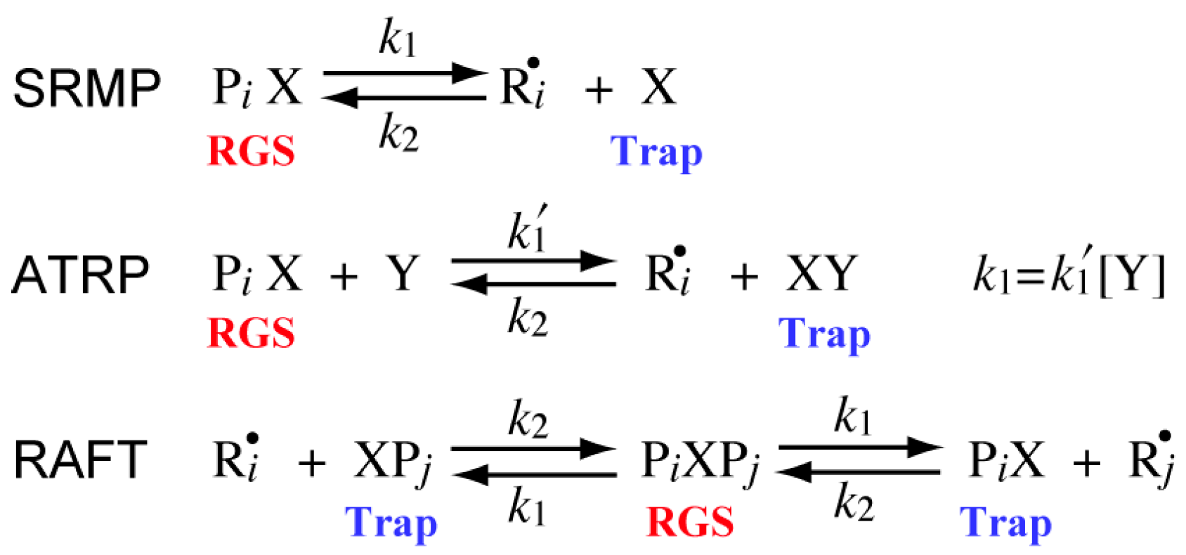
Figure 1 shows the reversible deactivation reactions in some of representative RDRPs, i.e., stable-radical-mediated polymerization (SRMP), atom-transfer radical polymerization (ATRP), and reversible-addition-fragmentation chain-transfer (RAFT) polymerization. In order to formulate the polymerization rate expression for various types of RDRPs in a unified manner [22], the component that generates an active radical is represented as the radical generating species (RGS), and the component that deactivates an active radical is represented as the trapping agent (Trap) in Figure 1.
In order to highlight the most fundamental characteristics in living emulsion FRP, an ideal living radical polymerization, with no termination occurring other than the loss of livingness through the chain transfer to polymer is considered. Using the notations shown in Figure 1, the deactivation rate, Rdeact is given by:
Rdeact = k2 [Trap][R•].
Dividing Equation (7) by the polymerization rate, Rp = kp[M][R•], one obtains the following dimensionless ratio, δ:
δ = (k2 [Trap])/(kp [M]).
In emulsion polymerization, the monomer concentration in the polymer particle, [M]p is approximately constant until the depletion of monomer droplets. The value of [Trap]p may change even for a constant polymer/monomer ratio period in emulsion polymerization. However, in order to simplify the discussion, the value of δ is assumed constant during the polymerization in the present MC simulation.
Neglecting the bimolecular termination reactions, the probability that an active radical connects another monomer unit during the active period is given by:
Note that the rate ratio CP, defined by Equation (3), is constant, and therefore p is also a constant.
p = 1/(1 + δ + Cp).
The number-based chain length distribution during a single active period, Nsa(r) is given by the following modified most probable distribution [23]:
which includes the possibility that the activated species fails to connect a single monomer, i.e., the cases with r = 0. In this article, the sequence of monomeric units formed during a single active period is called a “segment chain.”
Nsa(r) = pr (1 − p),
The number-average chain length of segment chains, n,s is given by:
The probability that the active period starts from a midchain radical, which is equal to the probability that the chain end of a segment is connected to a backbone chain, Pbs is given by:
Pbs = CP/(δ + Cp).
Note that the “slow reactivation” of midchain dormant [24] is not considered in the present investigation, to highlight pure differences of living and nonliving FRP.
In order to make “fair” comparison with the corresponding conventional (nonliving) FRP, the final number-average chain length (degree of polymerization), n and the total number of monomeric units bound into polymer molecules in a particle, NM are set to be the same for both cases. The number of dormant species in a particle, which is equal to the number of product polymers in a particle, is given by NM/n. In the simulation for conventional FRP, a single linear polymer molecule having chain length ca. n,p exists initially. In order to have an equivalent initial condition for living FRP, the total of n,p/n,s dormant chains are generated. The chain lengths of these dormant chains are determined by generating random numbers that follow the distribution given by Equation (10), which can be done by using a uniform random number y between 0 and 1, as follows:
r = Ceiling[ln y/ln p − 1].
The MC simulation starts from the following initial condition. There are n,p/n,s dormant chains whose lengths are generated by using Equation (13), and (NM/n − n,p/n,s) dormant species having length 0 in a polymer particle. Note in the present simulation study shown in the next section, NM/n > n,p/n,s for all conditions. After that, one chain end having a trapping agent is selected randomly to be activated, and a new segment chain, generated by using Equation (13), is connected to the activated chain end. Then, with probability (1 − Pbs), the eliminated trapping agent is attached to the segment end. On the other hand, with probability Pbs, chain transfer to polymer occurs, and the location of a midchain radical is determined by selecting one unit randomly from the already formed chains. In this case, next segment grows from the midchain radical to form a branch chain and the eliminated trapping agent moves to be attached to this segment end. These processes continue until the total number of polymerized monomeric units leaches NM, and the simulation for a single particle ends. By repeating such simulation for a large number of polymer particles, one can determine the statistical properties of the product living polymers effectively.
3. Results and Discussion
The total number of monomeric units bound into polymer molecules in a particle, NM that defines the end point for the MC simulation is set to be NM = 1 × 10⁶ both for the conventional and living FRP. Assuming that the molecular weight of monomer is 100 and that the density of polymer is 1 g/cm3, the value of NM = 1 × 10⁶ corresponds to the diameter of the dried polymer particle being 68 nm. It is assumed that the polymer/monomer ratio in the polymer particle is kept constant until the end point of simulation, NM = 1 × 10⁶.
The parameters used for the conventional FRP are shown in Table 1, and those for the living FRP are shown in Table 2. The number-average chain length of the product polymers, n is 200 for C1 and L1, n = 500 for C2 and L2, and n = 1000 for C3, C4, L3, L4. Note that the number-average chain length, n is given by the following equation for the conventional FRP:
Because the polymer/monomer ratio, [P]p/[M]p is kept constant, the average branching density of the all polymers, is given by the following equation for both conventional and living FRP.
Table 3 shows the properties of product polymers that are set to be the same for the corresponding conventional and living FRP. For the living FRP, the probability that the chain end of a primary chain is connected, or the branching probability Pb, is not the same for all primary chains. However, the average branching probability, b is set to be the same for the corresponding conventional and living FRP, and b is increased from 0.2857 for C1 and L1 to 0.8333 for C4 and L4. In the case of living FRP, the number-average segment length during a single active period is set to be n,s = 2 throughout the polymerization.
3.1. Weight Fraction Distribution
3.1.1. Conventional Free-Radical Emulsion Polymerization
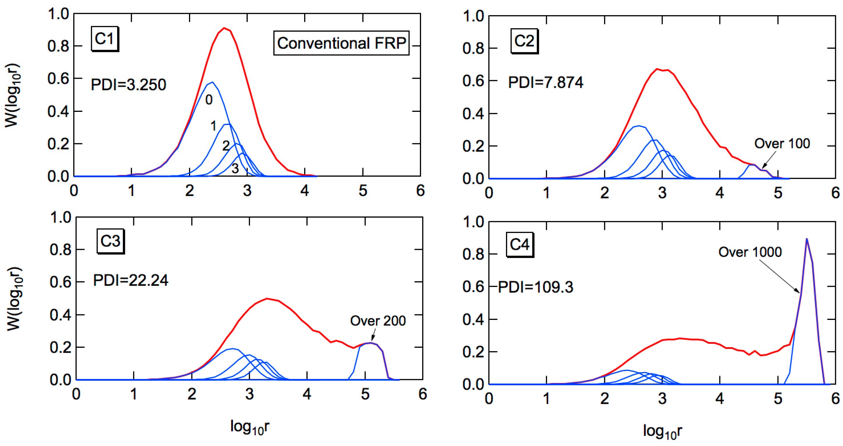
The red curve in Figure 2 shows the MC simulation results for the weight fraction distribution. The independent variable is the logarithm of chain length, as is usually employed for the GPC measurement. The blue curves in Figure 2 show the fractional MWDs consisting of k branch points. The value of k is 0, 1, 2, 3 from the left to the right. For the second high MW peak shown in C2–C4, the large k-value fractions are summed up, as shown in the figure. When the branching probability, Pb is large, a sharp high MW peak appears. In the present condition, the total number of monomeric units incorporated into polymer molecules is, NM = 1 × 10⁶, and therefore, a polymer molecule with log10r > 6 cannot exist in a polymer particle. The sharp high MW peak is formed due to the limitation of the small particle size. A sharp high MW peak essentially consists of the largest polymer molecule in each polymer particle [17].
In the present model emulsion polymerization, the weight-average chain length (degree of polymerization), w is given by [16,17]:
and
where n is the number of primary chains in a particle.
Table 4 shows the comparison of average chain lengths between the MC simulation results and the theoretical values. The errors are rather small, and the accuracy of the present MC simulation is confirmed. Note that the present MC simulation is conducted on the number basis, and therefore, the statistical errors are expected to be smaller for the number-average chain length n, rather than the weight-average w.
In order to highlight the characteristics of the emulsion polymerization system, the comparison with the random branched polymer, in which the probability of having a branch point ρ is the same for monomeric units in polymer, is considered. Suppose we have the primary chains whose number- and weight-average chain lengths are n,p and w,p, respectively. When such primary chains are connected through random branching, the number- and weight-average chain length are given, respectively, by [25]:
Note that Equations (18) and (19) are valid irrespective of the primary chain length distribution.
Comparison of the present model emulsion polymerization and random branching is shown in Table 5. The number-average chain length n is the same for both the emulsion polymers and the random branched polymers, because the average branching density is the same. On the other hand, in the case of the emulsion polymers, the expected branching density of the primary chains formed in the earlier stage of polymerization is much larger than those formed in the later stage of polymerization [5]. The primary chains with larger values of branching density form hubs in the buildup process to connect a large number of primary chains in a polymer molecule, which allows the formation of large sized polymers. It is clearly shown that the weight-average chain length w is larger for the emulsion polymers, especially for the large branching probability cases.
In the present model emulsion polymerization, the primary chain length distribution follows the most probable distribution, given by Equation (1). When the primary chains conforming to the most probable distribution are connected through random branching, the full weight fraction distribution can be calculated from the following equation [25]:
where I1 is the modified Bessel function of the first kind and of the first order.
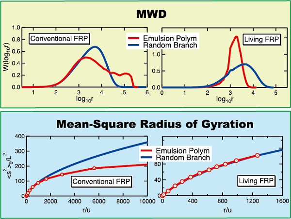
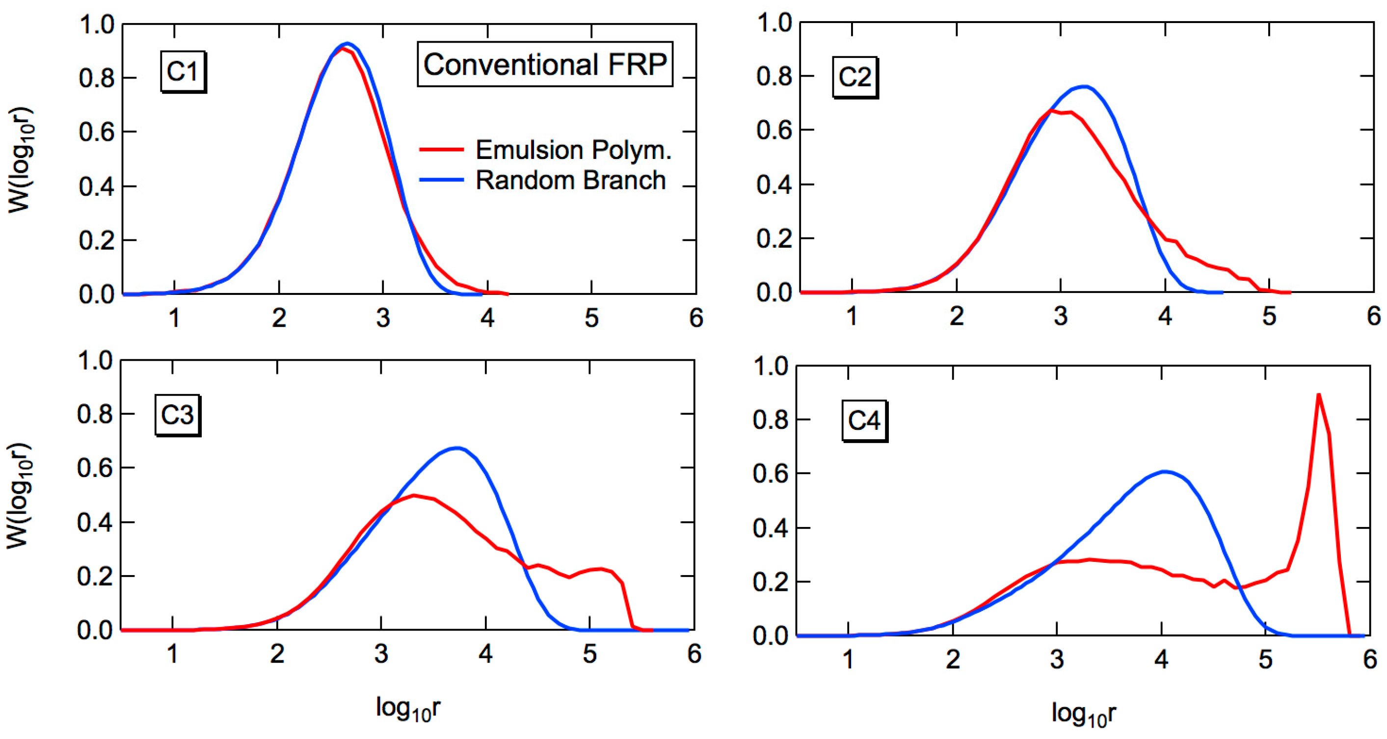
Figure 3 shows the comparison of the full weight fraction distribution profiles between the emulsion polymers and the random branched polymers. It is clearly shown that the MWD is much broader for the emulsion polymerization.
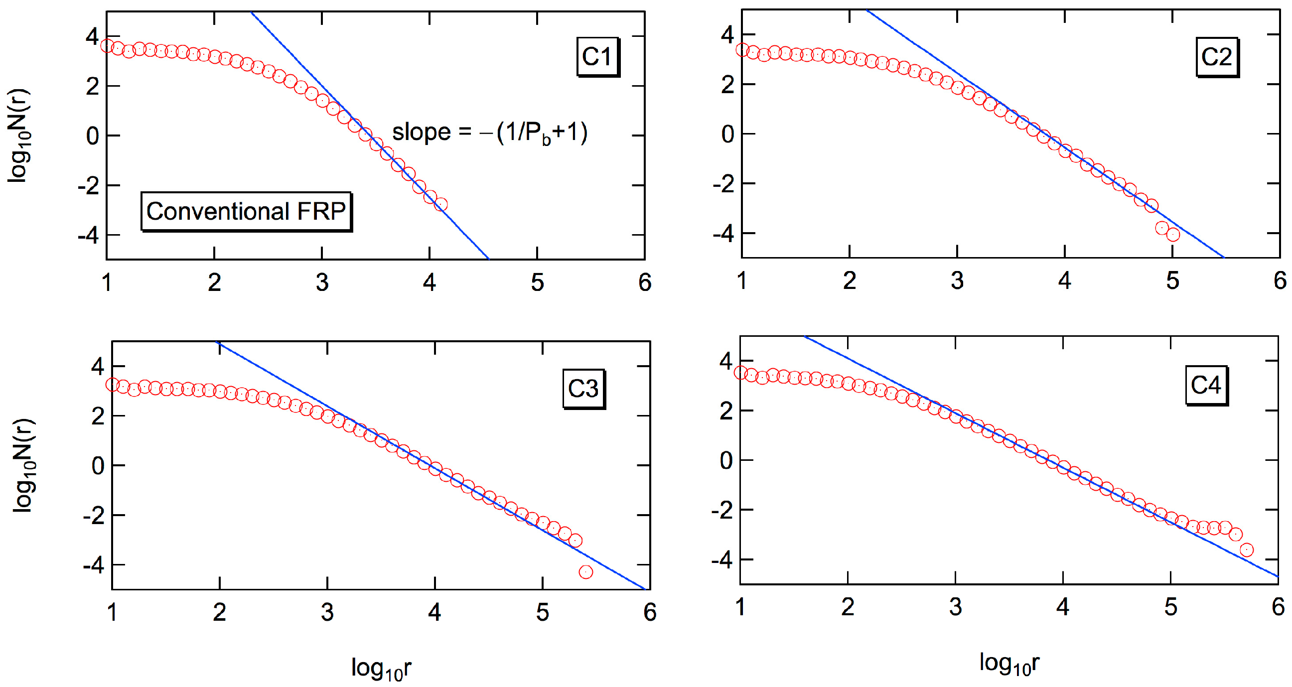
Figure 4 shows the log-log plot of the number fraction distribution, N(r). The power law holds for a significant range of chain lengths [8,18,19]. The power exponent for the number fraction distribution, N(r) is −(1/Pb + 1), as shown in the figure. With the relationship, W(r) ~ rN(r), the power exponent of the weight fraction distribution, W(r) is −1/Pb, i.e., W(r) ~ r−α with α = 1/Pb. Because the branching probability, Pb is related with the chain transfer constant Cfp through Equations (3) and (5), the value of Cfp could be estimated through the present type of double logarithmic plot, as was illustrated for the emulsion-polymerized polyethylene [18].
3.1.2. Living Free-Radical Emulsion Polymerization
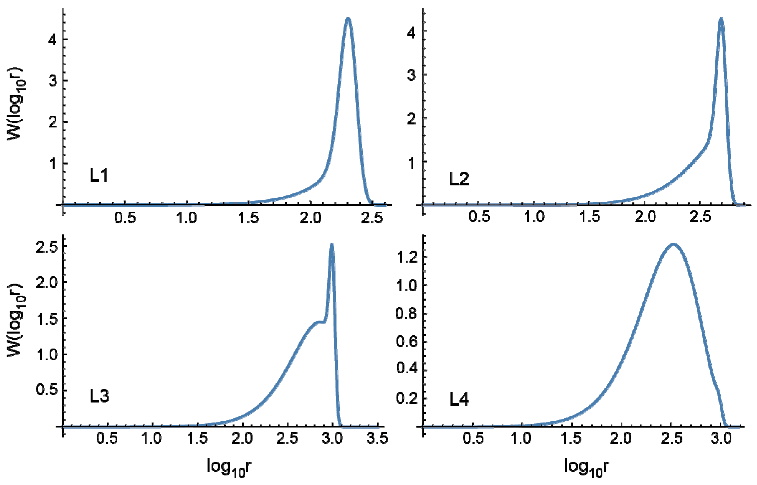
Figure 5 shows the MC simulation results for the full weight fraction distribution, formed through living FRP. A notable difference from the conventional FRP, shown in Figure 2, is the narrowness of the MWD. Note that the number-average chain length of primary chains n,p and the average branching density , as well as the number-average chain lengths of the product polymers n, are the same for the corresponding polymerization conditions, i.e., C1 and L1, C2 and L2, and so on. Bimodal distributions of W(log10r) are shown for L1 and L2. On the other hand, in the present idealized model, a uniform particle size distribution is assumed. In a real system, the MWD is expected to be somewhat broader than the present prediction, and the second peak may be difficult to be observed. In addition, the second peak contains branches and the hydrodynamic volume becomes smaller than the corresponding linear polymers. The peak separation could be difficult in the usual GPC analysis.
The power-law relationship of MWD was found for the conventional emulsion FRP, as was discussed in the previous section. On the other hand, the power law does not hold for the living emulsion polymerization.
In L4, the PDI value is 2.15, while the corresponding conventional FRP gives the PDI value as large as 109.3. In the cases of conventional emulsion FRP, the existence of long-chain branches would be predicted easily judging from a broad MWD. On the other hand, for living emulsion polymerization, the existence of long-chain branches could be overlooked because of a relatively narrow MWD of product polymers.
In Figure 5, the fractional MWDs containing k branches are also shown. Compared with the fractional MWDs for the conventional FRP shown in Figure 2, one would notice that the branch points are distributed much more equally for the living emulsion polymerization. Note that the average branching density of the whole system is the same for the corresponding conditions, e.g., C1 and L1, and so on, as shown in Table 3.
The MWD of linear polymer fraction (k = 0) shows a long tail toward small chain lengths. The long tail is formed through chain transfer to polymer, which causes irreversible deactivation of the chain-end radical. The primary chain length distribution in the present living polymerization system can be calculated theoretically, as follows.
In the case of ideal linear living FRP, where the segment distribution is kept constant throughout the polymerization without termination and chain transfer reactions, the full weight fraction distribution is given by [23]:
where F[a,b;x] is the confluent hypergeometric function (Kummer’s function of the first kind), and z is the average number of active period for a chain that is defined by:
Note that n,s = 2 in the present set of simulations.
In the present model reaction system, the probability for an active radical to cause chain transfer reaction, resulting in the irreversible termination for the primary chain is equal to CP, represented by Equation (3), which is kept constant throughout polymerization. When the ideal living chains whose MWD is represented by Equation (21) is subjected to a constant probability of chain transfer, the weight fraction distribution is represented by [23]:
Equation (23) gives the weight fraction distribution of the primary chains in the present model living emulsion polymerization. Figure 6 shows the calculated results for L1 to L4. The characteristics of long tails in the low MW region, including a strange distorted fractional MWD profile for k = 0 of L3 condition in Figure 5, agree qualitatively with the primary chain length distribution shown in Figure 6. Note that the primary chains whose distribution is given by Figure 6 are combined, according to the pertinent emulsion polymerization kinetics, to form the branched polymers whose MWD is shown in Figure 5.
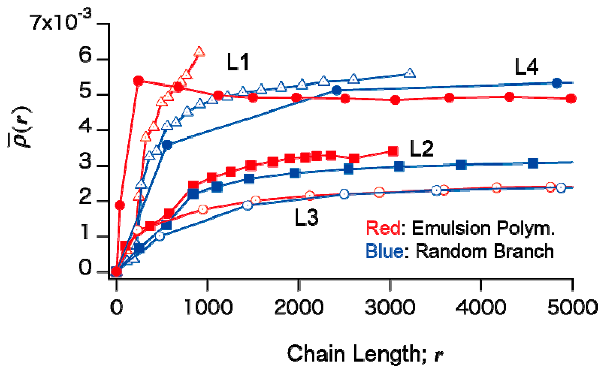
The number-average chain lengths of the primary chains, n,p for L1 to L4 are given respectively in Table 3. The weight-average chain lengths of the primary chains, w,p can be calculated from Equation (23). On the other hand, if these primary chains are combined to form random branched polymers, the number- and weight-average chain lengths of product polymers can be calculated from Equations (18) and (19). Note that Equations (18) and (19) are valid, irrespective of the primary chain length distribution, as long as the branching is random, i.e., the probability of having a branch point is the same for all units.
Table 6 shows the comparison between the emulsion polymerization and the random branching, in the case of living FRP. The number-average chain length n is the same for both types of branched polymers, because the average branching density is the same. On the other hand, in the case of living FRP, the branch chains must be formed after the formation of the backbone chain. The branch chain is allowed to grow a shorter period of time than the backbone chain, and is expected to be shorter than the backbone chain. In addition, the branch chains formed later are subjected to branching reaction for a shorter period of time, and therefore, the expected branching density is smaller. On the other hand, in the random branched polymers, the expected branching density is the same for all primary chains and any primary chain can become a branch chain. A long primary chain having large branching density could be connected as a branch chain in the random branching process. Larger polymer molecules can be formed in the random branching process, compared with the living emulsion polymerization, leading to a larger weight-average chain length w. It is clearly shown that the living emulsion polymerization gives smaller PDI values, indicating narrower MWD.
The full weight fraction distribution of the random branched polymers, whose primary chain length distribution is given by Equation (23) can be determined by using the MC simulation. Figure 7 shows the comparison of weight fraction distribution, between random branching and emulsion polymerization. The formed MWDs in L1–L3 are distorted because of the complicated distribution of the primary chains. Both from the PDI values in Table 6 and the full MWD profiles in Figure 7, it can be concluded that the MWD is narrower for the emulsion-polymerized polymers, compared with the corresponding random branched polymers. Remember that for the conventional FRP, the results are totally opposite, i.e., the MWDs are much broader for the emulsion polymers, compared with random branching, in the case of conventional FRP.
3.2. Branching Density
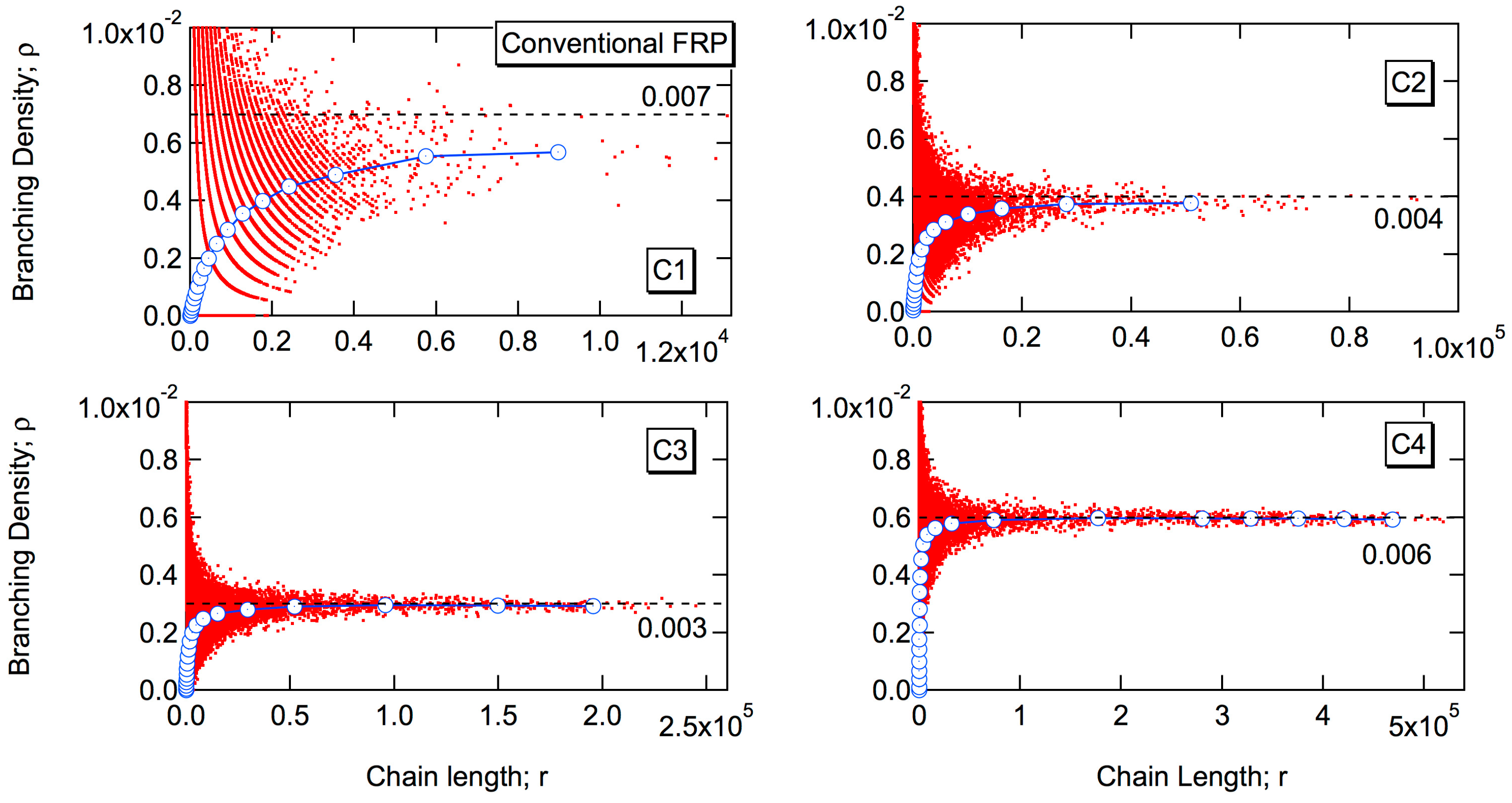
3.2.1. Conventional Free-Radical Emulsion Polymerization
Figure 8 shows the relationship between the branching density ρ and chain length r (degree of polymerization). In the figure, each dot represents the branching density and the chain length of each polymer molecule generated in the MC simulation. The blue curve shows the estimate of average branching density having chain length r, (r). As shown in the figure, the expected branching density increases as the chain length r increases for smaller polymers, but the value soon reaches a constant limiting value, . The branching densities of branched polymers are distributed around the value of , not the average branching density of the whole reaction system, given in Table 3. It is interesting to note that the high MW polymers that form the second sharp high MW peak of C3 and C4 in Figure 2 still possess the branching density approximately being equal to .
The black dotted line shows the value of 1/n,p, which seems to be a reasonable estimate of , at least for large branching probability cases, C2–C4.
Figure 9 shows the expected branching density of polymers having chain length r, (r). In the figure, the independent variable is changed to the reduced chain length defined by:
In addition, the y-axis in Figure 9 shows the product of (ζ) and n,p. For all 4 cases, including C1, the curves are reduced to fall approximately on the same curve. The number-average chain length of primary chains, n,p is kept constant throughout the polymerization in the present model emulsion polymerization, and therefore, the limiting value is given by:
It is now found that the limiting branching density is simply given by the inverse of the number-average chain length of the primary polymer molecules.
In the present model FRP, the primary chains conform to the most probable distribution. When the primary chains with the most probable distribution are branched randomly, the expected branching density, (r) is given by: [25]
or
where I2 is a modified Bessel function of the first kind of the second order, and Pb is the branching probability. For random branching, Pb = ρn,p.
Equation (27) shows that a universal curve exists for the relationship between (ζ)n,p and ζ, in the random branched polymer systems for a given branching probability, Pb. On the other hand, the value of Pb does not play a role in emulsion polymers, as shown in Figure 9.
From Equation (26), one can obtain the limiting branching density , as follows:
Because the value of Pb must be smaller than unity, i.e., Pb < 1, the limiting branching density, is always larger for the emulsion polymerization, compared with the corresponding random branched polymers. The lines in Figure 10 show the relationship between (ζ)n,p and ζ for the random branching, and that for the emulsion polymerization, in particular the data for C4. Although the emulsion polymerization shows slightly slower increase, but the limiting value, agrees with the case with Pb = 1 in the random branched polymer system.
In the present branched architecture, only one of two chain ends of a primary chain can be connected. In a branched polymer molecule, there always exists a single primary chain whose both chain ends are unconnected and all the other primary chains are connected at their head units. The branching density of a polymer molecule, consisting of k branch points and r monomeric units is given by:
where is the number-average chain length of the primary chains that constitute the branched polymer molecule. For large polymer, . Therefore, Equation (25) means to show that for large polymers in the conventional emulsion polymerization. For large emulsion polymers, no discrimination of the size of the primary chain exists in connecting branch chains. On the other hand, for the random branched polymers, , which means that larger primary chains are connected preferentially in the large-sized polymers.
3.2.2. Living Free-Radical Emulsion Polymerization
Figure 11 shows the relationship between the branching density and chain length for living free-radical emulsion polymerization. Each dot represents the branching density and the chain length of each polymer molecule generated in the MC simulation. The blue curve shows the estimate of the average branching density having chain length r, (r). The discrete arrays of dots correspond to the class of polymers having k = 0, 1, 2, … branch points. Because the number of “arrays” is small for L1 and L2, the curve for (r) is not smooth. It is interesting to note that in the case of L4, for which the average Pb-value is largest with b = 0.833 as listed in Table 3, the curve of (r) shows an overshooting behavior that was not observed in the conventional FRPs.
The black dotted lines in Figure 11 show the values of for the conventional emulsion polymerization. It is difficult to judge if these values apply also for living polymers, because the curve of (r) does not reach a constant value for L1 to L3. For L4, the limiting value for the living polymers, represented by the blue line, is clearly smaller than that for the corresponding conventional FRP given by the black dotted line. It seems that the limiting value, is close to the average branching density of the whole reaction system, that is = 0.005 given by the blue horizontal line.
Figure 12 shows the expected branching density, (r). The red lines are for the living emulsion polymerization, and the blue lines are for the random branched polymers whose primary chain length distribution is the same as for the corresponding living emulsion polymerization. For L1 and L2, the expected branching density of the large polymers seems to be larger for the emulsion polymers. On the other hand, however, the branching probability Pb is small for these conditions, and it is difficult to make discussions on the limiting branching density, . For L3, the limiting value seems to be almost the same, but the emulsion polymers show a larger branching density for the transient region of chain lengths. For L4, the branching density of the emulsion polymers is larger for smaller polymers, while it becomes smaller than the random branch for large chain length region. The behavior is quite complicated.
3.3. Radius of Gyration
In the present MC simulation method, one can observe the structure of each polymer molecule directly, and any type of detailed structural information can be extracted. The mean-square radius of gyration for the unperturbed random-flight chain of each polymer molecule, <s2>0 can be determined from the Wiener index (WI) [26]. The relationship between <s2>0 and WI is given by: [27]
where L is the random-walk segment length, and N is the number of random-walk steps in the given polymer. Obviously, N is given by:
where u is the number of monomeric units in a random-walk segment, and u = 5 was used for the actual calculation. Obviously, the “random-walk segment” is different from the “segment” introduced for the MC simulation of the living emulsion polymerization.
<s2>0/L2 = WI/N2,
N = r/u,
In the present simulation, the Wiener Index method is used for N < 1000. With the Wiener index method, the obtained mean-square radius of gyration is exact, with no statistical errors involved. The Wiener index method is an excellent method especially for smaller polymers whose standard deviation of <s2>0 in each polymer is large. For larger polymers with N > 1000, the actual random walk process in the 3D space was conducted for 100 times to estimate the value of <s2>0.
3.3.1. Conventional Free-Radical Emulsion Polymerization
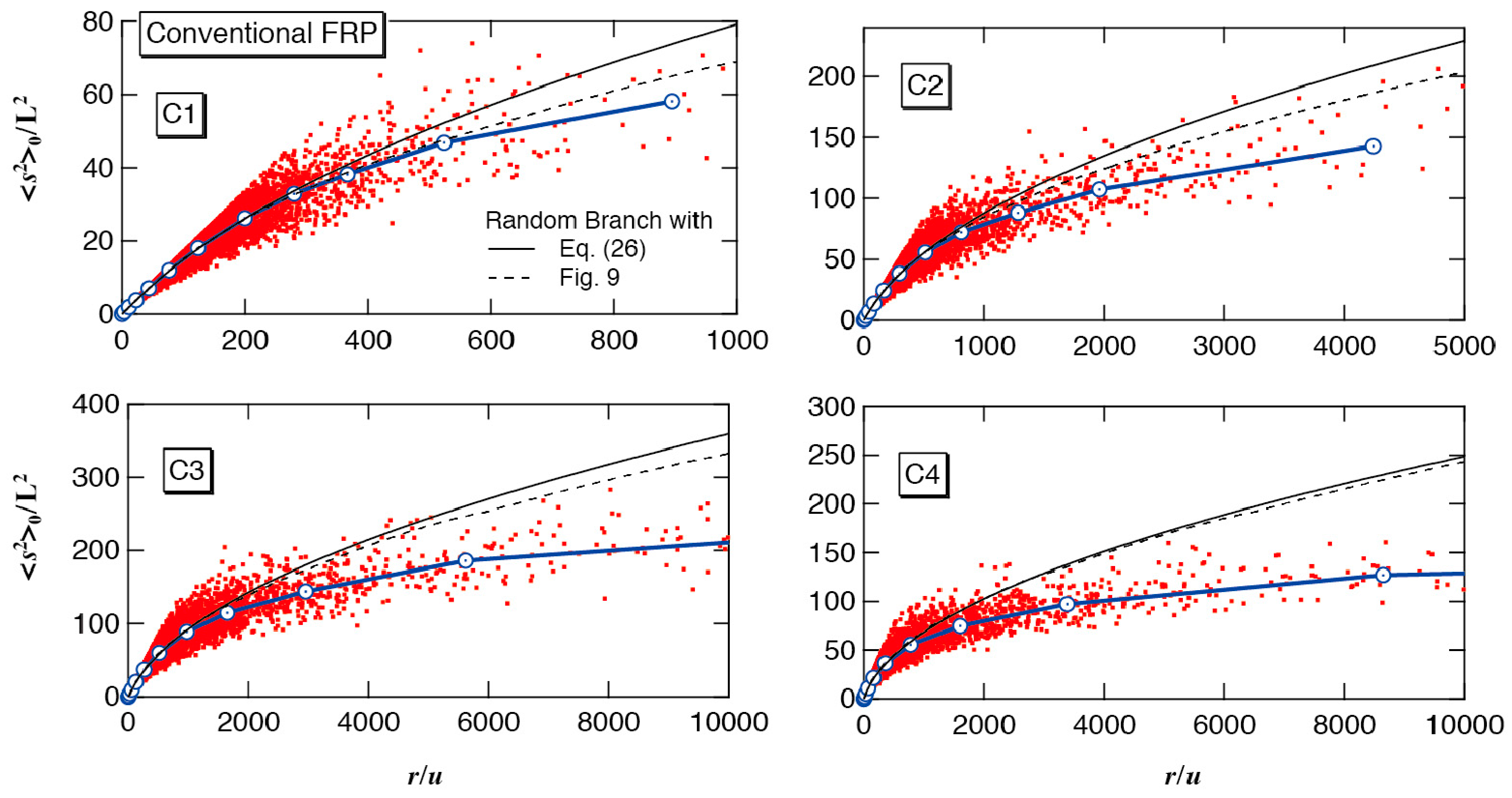
Figure 13 shows the relationship between the mean-square radius of gyration represented by <s2>0/L2 and chain length r divided by u. In the figure, each dot represents the value set of <s2>0/L2 and r/u of the individual polymer molecule obtained in the MC simulation, and the blue solid curve with circular symbols shows the average value of <s2>0/L2 within the intervals of Δr, which is the estimate of the average mean-square radius of gyration for the polymers having chain length r.
In Figure 13, the solid black curve shows the value of <s2>0/L2 for the random branched polymers whose primary polymer chain length distribution is the same as the present model emulsion polymers. For the random branched polymers whose primary chain length distribution conforms to the most probable distribution is given by [28]:
where r is the average number of branch points for the polymers with chain length r, which is given by:
In Equation (33), (r) is the average branching density of the polymer molecules having chain length r.
For a random branched polymer system whose primary chains conform to the most probable distribution, (r) is given by Equation (26), and the black solid curve shows such calculation results. It is clearly shown that the emulsion polymerization leads to more compact structure, compared with the random branched polymers.
On the other hand, however, the limiting branching density , or the branching density of large polymers is larger for the emulsion polymers, i.e., for the emulsion polymerization while for the random branching. Therefore, compact molecular architecture in emulsion polymerization might be resulted from larger branching density. In order to eliminate the factor of different branching density level, the expected branching density (r) shown by the blue curve in Figure 8 is used for Equation (33). The calculated results are shown by the black dotted curves in Figure 13. The ratio of limiting branching density between the emulsion polymerization and corresponding random branching is , and therefore, the difference between the black solid and dotted lines is large for C1 (Pb = 0.2857), and is small for C4 (Pb = 0.8333). In all cases, the expected mean-square radius of gyration is smaller for the emulsion polymers, which shows the non-randomness in the distribution of branch points formed in emulsion polymerization leads to compact 3D architecture in the conventional FRP.
In the conventional emulsion FRP, the expected branching density of the primary chains formed in the earlier stage of polymerization is much larger than those formed in the later stage of polymerization [5]. The primary chains with larger branching density form hubs to connect a large number of primary chains in a polymer molecule, leading to form a star-like compact architecture.
3.3.2. Living Free-Radical Emulsion Polymerization
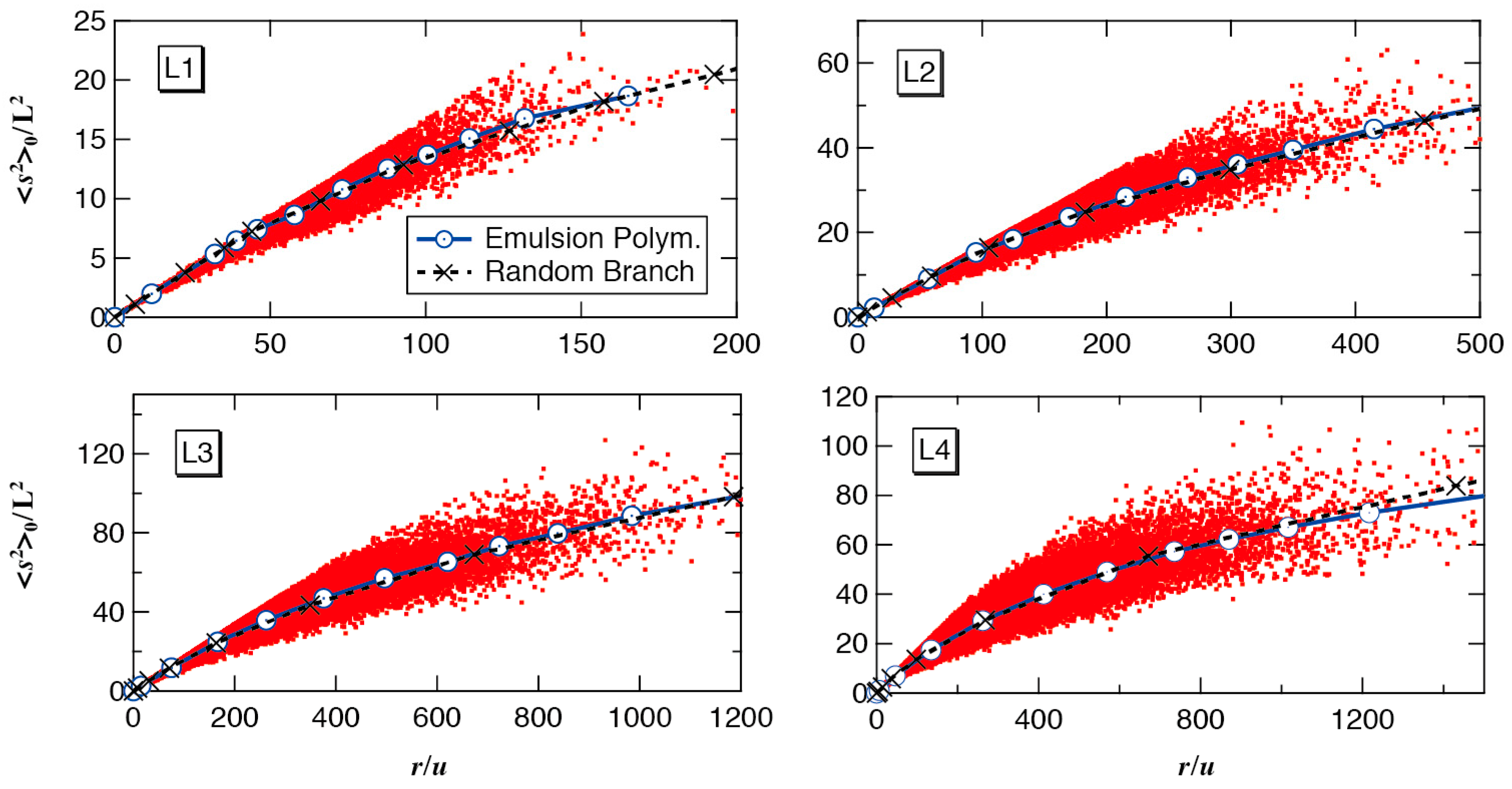
Figure 14 shows the relationship between the mean-square radius of gyration and chain length. Each red dot represents the mean-square radius of gyration of the individual polymer molecule obtained in the MC simulation, and the blue solid curve with circular symbols shows the estimate of the expected <s2>0 of polymers having chain length r.
The black dotted curve with X-symbols shows the value of <s2>0/L2 of the random branched polymers whose primary polymer chain length distribution, as well as the average branching density, is the same as the present model emulsion polymers. The mean-square radius of gyration of the random branched polymers was estimated by the MC simulation, in which the primary chains whose distribution is shown in Figure 6 are connected randomly. Interestingly, for living emulsion polymerization, the expected mean-square radius of gyration for the polymers with chain length r is essentially the same as for the random branched polymers.
4. Conclusions
Assuming an idealized emulsion polymerization condition, a Monte Carlo simulation is conducted for both conventional and living FRP, which involves chain transfer to polymer, resulting in forming polymers with long-chain branches.
The molecular weight distribution (MWD) of the emulsion polymers formed in conventional FRP is very broad, and high molecular weight polymers conform to the power law, W(r) = r−α with the power exponent α given by α = 1/Pb, where Pb is the probability that the chain end of the primary polymer molecule is connected to a backbone chain. The MWD is much broader than the corresponding random branched polymer system. When the branching probability Pb is large, the second sharp high MW peak appears because of the limitation of the particle size.
The MWD of emulsion polymers formed in living FRP is much narrower than that of the conventional FRP. The MWD is so narrow that one may overlook the existence of long-chain branches from the measured MWD data. The MWD is narrower than the corresponding random branched system.
The branching density of large polymers reaches a constant value, for both conventional and living emulsion FRPs, as well as for the random branched polymers. For the conventional FRP, a simple relationship, = 1/n,p is found. This limiting value is −times larger for the emulsion polymerization, compared with the corresponding random branched polymers.
For the living emulsion FRP, the relationship with the corresponding random branched polymers concerning the value of is rather complex, as was shown in Figure 12.
For the conventional emulsion FRP, the mean-square radii of gyration, <s2>0 for the given chain length r is smaller than the corresponding random branched polymers. On the other hand, for the living emulsion FRP, the value of <s2>0 for the given chain length r is essentially the same as for the random branched polymers.
The present model analysis promises to offer a broad perspective for designing and controlling the branched polymer architecture both in the conventional and living emulsion polymerization.
Conflicts of Interest
The author declares no conflict of interest.
Nomenclature
The following symbols and acronyms are used in this manuscript:
| Symbols | |
| [CTA]p | Concentration of the chain transfer agent in the polymer particle |
| CfCTA | Chain transfer constant to the chain transfer agent |
| Cfm | Chain transfer constant to monomer |
| Cfm | Chain transfer constant to polymer |
| CP | Ratio of the reaction rates between chain transfer to polymer and propagation |
| F[a,b;x] | Confluent hypergeometric function (Kummer’s function of the first kind) |
| I1 | Modified Bessel function of the first kind and of the first order |
| I2 | Modified Bessel function of the first kind and of the second order |
| k | Number of branch points in the polymer molecule |
| kp | Propagation rate constant |
| L | Random-walk segment length |
| [M]p | Monomer concentration in the polymer particle |
| r | Average number of branch points for the polymers with chain length r |
| N | Number of random-walk segments in the polymer |
| n | Number of primary chains in the particle |
| Npr(r) | Number-based chain length distribution of the primary chains |
| Nsa(r) | Number-based chain length distribution during a single active period in living FRP |
| N(r) | Number fraction distribution |
| p | Probability that an active radical connects another monomer unit during the active period in living FRP |
| Pb | Branching probability, which gives the probability that the chain end of a primary chain is connected to a backbone chain |
| Pbs | Probability that the chain end of a segment formed during a single active period is connected to a backbone chain in living FRP |
| [P]p | Polymer concentration in the polymer particle, represented by the total number of monomeric units in polymer |
| Rp | Polymerization rate |
| Rdeact | Deactivation rate in the reversible deactivation process in controlled/living radical polymerization |
| r | Chain length (number of monomeric units in the polymer) |
| n | Number-average chain length of the product polymers |
| n,p | Number-average chain length of the primary chains |
| Number-average chain length of the primary chains that constitute a branched polymer molecule | |
| n,s | Number-average chain length of the sequence of chains (segments) formed during a single active period in living FRP |
| w | Weight-average chain length of the product polymers |
| <s2>0 | Mean-square radius of gyration of unperturbed chain |
| tav | Average time interval between radical entry to a polymer particle |
| u | Number of monomeric units in a random-walk segment |
| WI | Wiener Index |
| W(r) | Weight fraction distribution |
| Wliv(r) | Weight fraction distribution of the ideal linear living FRP |
| WCP(r) | Weight fraction distribution of the polymer chains formed through the ideal linear living FRP with a constant chain transfer probability |
| y | Uniform random number between 0 and 1 |
| z | Average number of active period for the linear living chain formation |
| α | Exponent of the power-law distribution |
| δ | Ratio of the reaction rates between the deactivation in living FRP and the propagation, defined by Equation (8) |
| ζ | Reduced chain length, defined by r/n,p |
| ρ | Branching density |
| (r) | Expected branching density of the polymer molecules having chain length r |
| τ | Dimensionless parameter representing the ratio of reaction rates between various types of chain stoppage and the propagation, defined by Equation (2) |
| Acronyms | |
| ATRP | Atom-Transfer Radical Polymerization |
| CTA | Chain Transfer Agent |
| FRP | Free-Radical Polymerization |
| GPC | Gel Permeation Chromatography |
| MC | Monte Carlo |
| MW | Molecular Weight |
| MWD | Molecular Weight Distribution |
| PDI | Polydispersity Index, PDI = w/n |
| RAFT | Reversible Addition–Fragmentation Chain-Transfer |
| RDRP | Reversible-Deactivation Radical Polymerization |
| SRMP | Stable-Radical-Mediated Polymerization |
References
- Odian, G. Principles of Polymerization, 4th ed.; John Wiley & Sons: Hoboken, NJ, USA, 2004; pp. 252–255. [Google Scholar]
- Plessis, C.; Arzamendi, G.; Leiza, J.R.; Schoonbrood, H.A.S.; Charmot, D.; Asua, J.M. Seeded Semibatch Emulsion Polymerization of n-Butyl Acrylate. Kinetics and Structural Properties. Macromolecules 2000, 33, 5041–5047. [Google Scholar] [CrossRef]
- Nikitin, A.N.; Hutchinson, R.A.; Kalfas, G.A.; Richards, J.R.; Bruni, C. The effect of Intramolecular Transfer to Polymer on Stationary Free-Radical Polymerization of Alkyl Acrylates, 3—Consideration of Solution Polymerization up to High Conversions. Macromol. Theory Simul. 2009, 18, 247–258. [Google Scholar] [CrossRef]
- Tobita, H. Molecular Weight Distribution in Free Radical Polymerization with Long-Chain Branching. J. Polym. Sci. B Polym. Phys. 1993, 31, 1363–1371. [Google Scholar] [CrossRef]
- Tobita, H. Kinetics of Long-Chain Branching via Chain Transfer to Polymer: 1. Branched Structure. Polym. React. Eng. 1993, 1, 357–378. [Google Scholar] [CrossRef]
- Gilbert, R.G. Emulsion Polymerization, A Mechanistic Approach; Academic Press: San Diego, CA, USA, 1995. [Google Scholar]
- Tobita, H.; Yamamoto, K. Network Formation in Emulsion Cross-Linking Copolymerization. Macromolecules 1994, 27, 3389–3396. [Google Scholar] [CrossRef]
- Tobita, H. Scale-Free Power-Law Distribution of Emulsion Polymerized Nonlinear Polymers: Free-Radical Polymerization with Chain Transfer to Polymer. Macromolecules 2004, 37, 585–589. [Google Scholar] [CrossRef]
- Cunningham, M.F. Controlled/living radical polymerization in aqueous dispersed systems. Prog. Polym. Sci. 2008, 33, 365–398. [Google Scholar] [CrossRef]
- Zetterlund, P.B.; Kagawa, Y.; Okubo, M. Controlled/Living Radical Polymerization in Dispersed Systems. Chem. Rev. 2008, 108, 3747–3794. [Google Scholar] [CrossRef] [PubMed]
- Ferguson, C.J.; Hughes, R.J.; Nguyen, D.; Pham, B.T.T.; Gilbert, R.G.; Serelis, A.K.; Such, C.H.; Hawkett, B.S. Ab Initio Emulsion Polymerization by RAFT-Controlled Self-Assembly. Macromolecules 2005, 38, 2191–2204. [Google Scholar] [CrossRef]
- Luo, Y.; Wang, X.; Li, B.G.; Zhu, S. Toward Well-Controlled ab Initio RAFT Emulsion Polymerization of Styrene Mediated by 2-(((Dodecylsulfanyl)carbonothiol)sulfanyl)propanoic Acid. Macromolecules 2011, 44, 221–229. [Google Scholar] [CrossRef]
- Zhu, Y.; Bi, S.; Gao, X.; Luo, Y. Comparison of RAFT Ab Initio Emulsion Polymerization of Methyl Methacrylate and Styrene Mediated by Oligo(methacrylic acid-β-methyl methacrylate) Trithiocarbonate Surfactant. Macromol. React. Eng. 2015, 9, 503–511. [Google Scholar] [CrossRef]
- Gonzalez-Blanco, R.; Saldivar-Guerra, E.; Herrera-Ordonez, J.; Cano-Valdez, A. TEMPO Mediated Radical Emulsion Polymerization of Styrene by Stepwize and Semibatch Processes. Macromol. Symp. 2013, 325, 89–95. [Google Scholar] [CrossRef]
- Li, X.; Wang, W.J.; Li, B.G.; Zhu, S. Branching in RAFT Miniemulsion Copolymerization of Styrene/Triethylene Glycol Dimethacrylate and Contro of Branching Density Distribution. Macromol. React. Eng. 2015, 9, 90–99. [Google Scholar] [CrossRef]
- Tobita, H. Molecular Weight Distribution in Nonlinear Emulsion Polymerization. J. Polym. Sci. B Polym. Phys. 1997, 35, 1515–1532. [Google Scholar] [CrossRef]
- Tobita, H. Bimodal Molecular Weight Distribution Formed in Emulsion Polymerization with Long-Chain Branching. Polym. React. Eng. 2003, 11, 855–868. [Google Scholar] [CrossRef]
- Tobita, H. Scale-Free Power-Law Distribution of Emulsion Polymerized Branched Polymers: Power Exponent of the Molecular Weight Distribution. Macromol. Mater. Eng. 2005, 290, 363–371. [Google Scholar] [CrossRef]
- Tobita, H. Power-law distribution of molecular weights of nonlinear emulsion polymers. e-Polymers 2005, 5, 684–694. [Google Scholar] [CrossRef]
- Tobita, H. Polymerization Processes, 1. Fundamentals. In Ullmann’s Encyclopedia of Industrial Chemistry; Elvers, B., Ed.; Wiley: Weinheim, Germany, 2015. [Google Scholar] [CrossRef]
- Jenkins, A.D.; Jones, R.G.; Moad, G. Terminology for reversible-deactivation radical polymerization previously called “controlled” radical or “living” radical polymerization (IUPAC Recommendations 2010). Pure Appl. Chem. 2010, 82, 483–491. [Google Scholar] [CrossRef]
- Tobita, H. Effect of Small Reaction Locus in Free-Radical Polymerization: Conventional and Reversible-Deactivation Radical Polymerization. Polymers 2016, 8, 155. [Google Scholar] [CrossRef]
- Tobita, H. Molecular Weight Distribution of Living Radical Polymers. 1. Fundamental Distribution. Macromol. Theory Simul. 2006, 15, 12–22. [Google Scholar] [CrossRef]
- Konkolewicz, D.; Sosnowski, S.; D’hooge, D.R.; Szymanski, R.; Reyniers, M.F.; Martin, G.B.; Matyjaszewski, K. Origin of the difference between Branching an Acrylates Polymerization under Controlled and Free Radical Conditions: A Computational Study of Competitive Processes. Macromolecules 2011, 44, 8361–8373. [Google Scholar] [CrossRef]
- Tobita, H. Molecular weight distribution in random branching of polymer chains. Macromol. Theory Simul. 1996, 5, 129–144. [Google Scholar] [CrossRef]
- Wiener, H. Structural Determination of Paraffin Boiling Points. J. Am. Chem. Soc. 1947, 69, 17–20. [Google Scholar] [CrossRef] [PubMed]
- Nitta, K. A topological approach to statistics and dynamics of chain molecules. J. Chem. Phys. 1994, 101, 4222–4228. [Google Scholar] [CrossRef]
- Zimm, G.H.; Stockmayer, W.H. The dimensions of chain molecules containing branches and rings. J. Chem. Phys. 1949, 17, 1301–1314. [Google Scholar] [CrossRef]
Figure 1.
Reversible deactivation reactions in some of representative RDRP. In the figure, PiX or XPi is the dormant polymer with chain length i. is the active polymer radical with chain length i.
Figure 1.
Reversible deactivation reactions in some of representative RDRP. In the figure, PiX or XPi is the dormant polymer with chain length i. is the active polymer radical with chain length i.

Figure 2.
Weight fraction distribution determined by the MC simulation for the conditions, C1–C4. In the figure, PDI means the polydispersity index, defined by PDI = w/n. The PDIs are the theoretical values, with w being calculated from Equations (16) and (17).
Figure 2.
Weight fraction distribution determined by the MC simulation for the conditions, C1–C4. In the figure, PDI means the polydispersity index, defined by PDI = w/n. The PDIs are the theoretical values, with w being calculated from Equations (16) and (17).

Figure 3.
Comparison of the full weight fraction distribution profiles of polymers formed through the conventional emulsion polymerization for the conditions, C1–C4 (red) and the corresponding random branching (blue).
Figure 3.
Comparison of the full weight fraction distribution profiles of polymers formed through the conventional emulsion polymerization for the conditions, C1–C4 (red) and the corresponding random branching (blue).

Figure 4.
Double logarithmic plot of the number fraction distribution of the polymers formed through the conventional free-radical emulsion polymerization, for the conditions C1–C4.
Figure 4.
Double logarithmic plot of the number fraction distribution of the polymers formed through the conventional free-radical emulsion polymerization, for the conditions C1–C4.

Figure 5.
Weight fraction distribution determined by the MC simulation for the living emulsion polymerization, for the conditions, L1–L4. The PDI values in the figure are determined also from the MC simulation results.
Figure 5.
Weight fraction distribution determined by the MC simulation for the living emulsion polymerization, for the conditions, L1–L4. The PDI values in the figure are determined also from the MC simulation results.
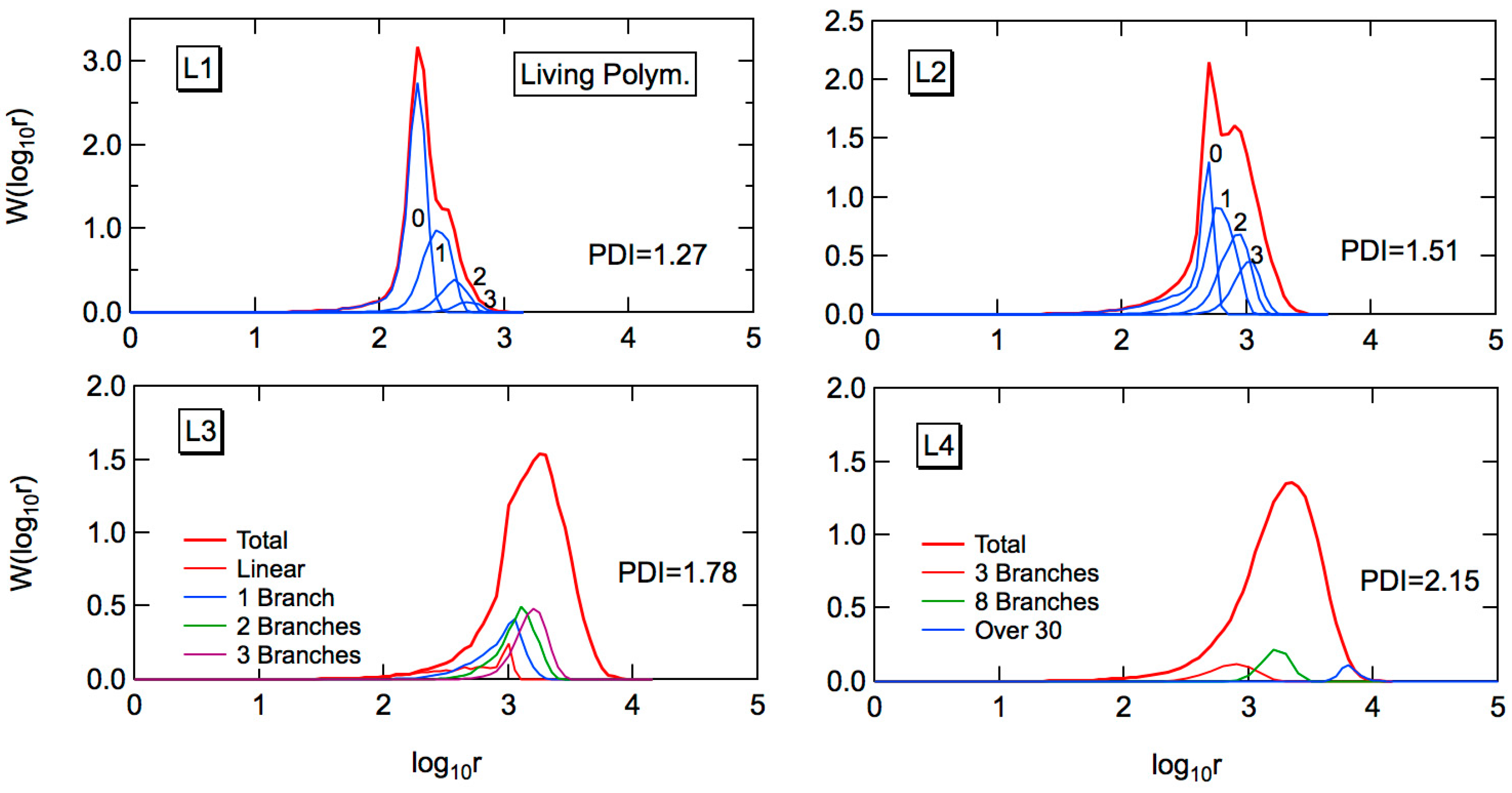
Figure 6.
Primary polymer chain length distribution of the present model living emulsion polymerization for the conditions L1–L4, calculated from Equation (23).
Figure 6.
Primary polymer chain length distribution of the present model living emulsion polymerization for the conditions L1–L4, calculated from Equation (23).

Figure 7.
Comparison of the full weight fraction distribution profiles formed through the living emulsion polymerization for the conditions L1–L4 (red) and the corresponding random branching (blue).
Figure 7.
Comparison of the full weight fraction distribution profiles formed through the living emulsion polymerization for the conditions L1–L4 (red) and the corresponding random branching (blue).
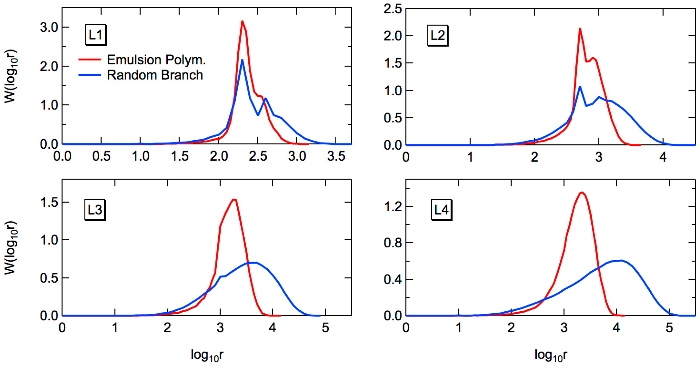
Figure 8.
Relationship between branching density and chain length in conventional free-radical emulsion polymerization, for the conditions C1–C4.
Figure 8.
Relationship between branching density and chain length in conventional free-radical emulsion polymerization, for the conditions C1–C4.

Figure 9.
Expected branching density of the polymer whose reduced chain length is ζ (= r/n,p).

Figure 10.
Expected branching density of the polymer whose reduced chain length is ζ (=r/n,p). The lines are for random branching with the given Pb-values, and the circular symbols are for the conventional emulsion polymerization, C4.
Figure 10.
Expected branching density of the polymer whose reduced chain length is ζ (=r/n,p). The lines are for random branching with the given Pb-values, and the circular symbols are for the conventional emulsion polymerization, C4.
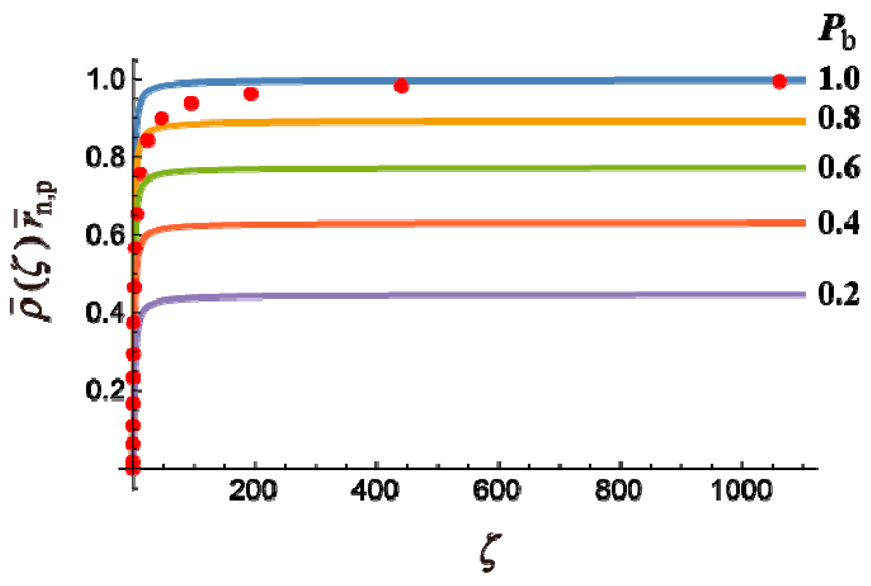
Figure 11.
Relationship between the branching density and the chain length in living free-radical emulsion polymerization, for the conditions L1–L4.
Figure 11.
Relationship between the branching density and the chain length in living free-radical emulsion polymerization, for the conditions L1–L4.

Figure 12.
Expected branching density of the polymer with chain length r, for living emulsion polymerization (red) and random branching (blue).
Figure 12.
Expected branching density of the polymer with chain length r, for living emulsion polymerization (red) and random branching (blue).

Figure 13.
Relationship between the mean-square radius of gyration, <s2>0 and the chain length, r for the conventional emulsion polymerization conditions, C1–C4. The red dots show the property of each polymer molecule simulated, and the blue curve with circular symbols is the expected <s2>0–value for the given r. The black solid and dotted curves are for the random branched polymers, having the same primary chain length distribution. See more details in the text.

Figure 14.
Relationship between the mean-square radius of gyration, <s2>0 and the degree of polymerization, r for the living emulsion polymerization conditions, L1–L4. The red dots show the property of each polymer molecule simulated, and the blue curve with circular symbol is the expected <s2>0–value for the given r. The black dotted curve with -symbol is for the random branched polymers, having the same primary chain length distribution and the average branching density.


Table 1.
Parameters used for conventional FRP.
| Run | τ | CP |
|---|---|---|
| C1 | 0.005 | 0.002 |
| C2 | 0.002 | 0.002 |
| C3 | 0.001 | 0.002 |
| C4 | 0.001 | 0.005 |
Table 2.
Parameters used for living FRP.
| Run | 1/n | CP |
|---|---|---|
| L1 | 0.005 | 0.002 |
| L2 | 0.002 | 0.002 |
| L3 | 0.001 | 0.002 |
| L4 | 0.001 | 0.005 |
n,s = 2 for all cases, which means that p = 2/3.
Table 3.
Properties set to be the same for the corresponding conventional and living FRP.
| Run | n | n,p 1) | b 2) | |
|---|---|---|---|---|
| C1, L1 | 200 | 0.002 | 142.9 | 0.2857 |
| C2, L2 | 500 | 0.002 | 250 | 0.5 |
| C3, L3 | 1000 | 0.002 | 333.3 | 0.6667 |
| C4, L4 | 1000 | 0.005 | 166.7 | 0.8333 |
1) The primary chains are defined as linear chains when the branch points formed by chain transfer to polymer are severed, both for the conventional and living FRP, which is given by 1/n,p = 1/n + CP. 2) Average probability for the chain end of a primary chain is connected to a backbone chain, which is given by b = n.
Table 4.
Comparison of the calculated average chain lengths.
| Run | Description | n | w |
|---|---|---|---|
| C1 | MC | 200.6 | 647.9 |
| Theory | 200 | 649.9 | |
| Error (%) | 0.3 | −0.311 | |
| C2 | MC | 500.3 | 4024.5 |
| Theory | 500 | 3936.8 | |
| Error (%) | 0.06 | 2.23 | |
| C3 | MC | 1000.4 | 21,753.9 |
| Theory | 1000 | 22,238.4 | |
| Error (%) | 0.04 | −2.18 | |
| C4 | MC | 1001.9 | 108,989 |
| Theory | 1000 | 109,270 | |
| Error (%) | 0.19 | −0.257 |
Table 5.
Comparison of the calculated average chain lengths for conventional FRP.
| Run | Description | n | w | PDI |
|---|---|---|---|---|
| C1 | Emulsion Polym. | 200 | 649.9 | 3.250 |
| Random Branch | 200 | 560 | 2.8 | |
| C2 | Emulsion Polym. | 500 | 3936.8 | 7.874 |
| Random Branch | 500 | 2000 | 4 | |
| C3 | Emulsion Polym. | 1000 | 22,238.4 | 22.24 |
| Random Branch | 1000 | 6000 | 6 | |
| C4 | Emulsion Polym. | 1000 | 108,989 | 109.3 |
| Random Branch | 1000 | 12,000 | 12 |
Table 6.
Comparison of the calculated average chain lengths for living FRP.
| Run | Description | n | w | PDI |
|---|---|---|---|---|
| L1 | Emulsion Polym. | 200 | 254.2 | 1.27 |
| Random Branch | 200 | 351.1 | 1.76 | |
| L2 | Emulsion Polym. | 500 | 755.8 | 1.51 |
| Random Branch | 500 | 1478.9 | 2.96 | |
| L3 | Emulsion Polym. | 1000 | 1782.3 | 1.78 |
| Random Branch | 1000 | 5115.1 | 5.12 | |
| L4 | Emulsion Polym. | 1000 | 2153.3 | 2.15 |
| Random Branch | 1000 | 11,540.9 | 11.5 |
© 2018 by the author. Licensee MDPI, Basel, Switzerland. This article is an open access article distributed under the terms and conditions of the Creative Commons Attribution (CC BY) license (http://creativecommons.org/licenses/by/4.0/).
Share and Cite
MDPI and ACS Style
Tobita, H. Effect of Chain Transfer to Polymer in Conventional and Living Emulsion Polymerization Process. Processes 2018, 6, 14. https://doi.org/10.3390/pr6020014
AMA Style
Tobita H. Effect of Chain Transfer to Polymer in Conventional and Living Emulsion Polymerization Process. Processes. 2018; 6(2):14. https://doi.org/10.3390/pr6020014
Chicago/Turabian StyleTobita, Hidetaka. 2018. "Effect of Chain Transfer to Polymer in Conventional and Living Emulsion Polymerization Process" Processes 6, no. 2: 14. https://doi.org/10.3390/pr6020014
Note that from the first issue of 2016, this journal uses article numbers instead of page numbers. See further details here.