Predicting the Operating States of Grinding Circuits by Use of Recurrence Texture Analysis of Time Series Data


1
Department of Mining Engineering and Metallurgical Engineering, Western Australian School of Mines, Curtin University, GPO Box U1987, Perth, 6845 WA, Australia
2
Department of Chemical Engineering, Curtin University, GPO Box U1987, Perth, 6845 WA, Australia
*
Author to whom correspondence should be addressed.
Processes 2018, 6(2), 17; https://doi.org/10.3390/pr6020017
Submission received: 28 December 2017
/
Revised: 24 January 2018
/
Accepted: 29 January 2018
/
Published: 11 February 2018
(This article belongs to the Collection Process Data Analytics)
Abstract
:Grinding circuits typically contribute disproportionately to the overall cost of ore beneficiation and their optimal operation is therefore of critical importance in the cost-effective operation of mineral processing plants. This can be challenging, as these circuits can also exhibit complex, nonlinear behavior that can be difficult to model. In this paper, it is shown that key time series variables of grinding circuits can be recast into sets of descriptor variables that can be used in advanced modelling and control of the mill. Two real-world case studies are considered. In the first, it is shown that the controller states of an autogenous mill can be identified from the load measurements of the mill by using a support vector machine and the abovementioned descriptor variables as predictors. In the second case study, it is shown that power and temperature measurements in a horizontally stirred mill can be used for online estimation of the particle size of the mill product.
1. Introduction
Energy consumption in comminution circuits is often the single largest component of the energy expenditure in concentrator circuits, owing to the inefficiency of the processes used to reduce the size of ore particles [1], among other reasons. Considerable effort has been expended to increase the efficiency of grinding circuits by improvements in the design of comminution equipment, as well as smarter operation or better control of operations [2]. The limited availability of reliable models is a significant and ongoing challenge in these efforts, as comminution circuits can exhibit complex nonlinear behavior that can be difficult to capture in first-principles models [2].
As a result, the use of data-based process models is increasingly attracting attention, as data are becoming abundant and the means to process these data are likewise becoming increasingly sophisticated and cheap. Over the last decade, a number of studies have appeared in this regard, e.g., in the analysis of vibration and acoustic signals from comminution equipment [3,4,5,6,7], estimation of mill load parameters [8,9], and soft sensor approaches to the monitoring of mill operations [10].
In many of these studies, nonlinear time series analysis, in one form or another, plays a critical role; in this investigation, a novel approach to nonlinear time series analysis is proposed and is used to explore the behavior of grinding equipment. The proposed method is based on the analysis of the structures or patterns in time series data by extracting features representing the Euclidean distances between the time series measurements.
These distances are collected in a matrix that is amenable to analysis by a large body of multivariate methods. As demonstrated in this paper, it includes the use of textural analysis, whereby information-rich descriptors of the dynamics of the comminution equipment can be extracted. These descriptors can subsequently be used as predictors in process models or to visualize the behavior of the equipment, as discussed in more detail in the paper.
2. Recurrence Texture Analysis of Time Series Data
A general overview of the analytical method is given in Figure 1. It starts by dividing the generally multivariate time series (A) into segments of equal lengths, specified by the user (B). A distance matrix is calculated for each time series segment (C) and, from this matrix, a set of features is extracted (D) that can subsequently be used for further analysis, such as predictors in a classification model (E). A more formal description follows below.
2.1. Segmentation of Time Series Data
In the first step, the normalized time series data consisting in total of observations, , are partitioned into a number of equal segments , where = 1, 2, …, . These segments each contain observations, as specified by the user. Ideally, each segment should be as short as possible, but still be of sufficient length to capture the characteristic or recurrent behavior of the time series. The latter requirement could, in principle, be accomplished by selecting a value for approximately coinciding with the first minimum point in the autocorrelation function (ACF) of the time series, as shown in Equation (1). In this equation, and are the sample (time series) mean and sample (time series) variance.
This approach is often used to estimate the minimum lag in a sense such that the time series and its lagged counterpart become independent of one another [11]. Alternatively, the value of can be determined empirically as a problem-dependent parameter that needs to be optimized over a certain range []. The minimum value of could theoretically not be less than 2, which would yield a window containing 2 or fewer samples and would thus preclude the calculation of a distance matrix, as discussed in Section 2.2.
2.2. Distance Matrix Calculation
Once the time series segmentation is completed, a distance matrix is computed for each time series segment , for . In this paper, the Euclidean distance metric is used, owing to its simple, yet competitive capability in dealing with time series classification [12]. The elements of the matrix are calculated according to Equation (2). This uses a Euclidean norm to calculate the proximity of a given point to another point . As a result, it forms a distance square using the equation below.
The textural analysis of image data is considered here to capture the structural information contained in the Euclidean distance matrices by considering these matrices as ‘images’ of the time series with their elements or values being the equivalent of image pixels.
Three different algorithms were implemented to extract features from the distance matrices, namely, textons, and two algorithms based on pretrained convolutional neural networks, namely, AlexNet and VGG16. These algorithms are described in more detail elsewhere and only briefly summarized below.
2.3. Texton Algorithm
Textons refer to fundamental microstructures or textural primitives in images, such as blobs, edges, line terminators, and line crossings, etc., and were conceptualized as the basis for an alternative texture perception model. According to this model, texture discrimination is governed by local processes, instead of a global process governed by well-defined higher-order statistical properties [13,14]. Discrimination between textures is based on local changes in pixel densities [14,15].
In general, textons are learned in a series of steps in a training stage that includes image filtering, filter response aggregation, and texton definition as cluster centers in the filter response space [16]. Textons are defined by performing vector quantization, e.g., k-means clustering, on the filtered responses of the images from the training set.
These responses are obtained through convolution of images in a training set with oriented linear spatial basis functions contained in a filter bank. For each training image , the number of pixels in the qth texton channel would provide the qth histogram bin in the image, . That is,
where and are the indicator function and the texton channel assigned to pixel j, respectively [17]. This histogram of textons is then considered to be the textural features extracted from the set of images [15,18]. In this study, these texton features are subsequently aggregated in a feature matrix , where is the number of time series segments, and is the number of texton features.
The textons were based on a Schmid filter bank [19] that uses a two-layer representation to capture ‘texture-like’ visual structures efficiently. The layers consist of descriptors and the joint probability of the frequencies of these over neighborhoods.
In essence, these descriptors are sets of rotationally invariant feature vectors, similar to a Gabor filter on the transformation of each pixel location, as indicated by Equation (4). The filter has complete rotational symmetry, but lacks sensitivity to anisotropic features [17].
In Equation (4), and are the x- and y-coordinates of the pixel in the image, is the cycle count in the harmonic function, and is the zero DC component guarantor. Note that to avoid high-frequency responses, a smaller is used at small scales.
2.4. AlexNet
A convolutional neural network typically consists of several groups of specialized layers. The first is an input layer, where data (images) are presented to the network. This layer is followed by convolutional layers containing fixed-sized filters that generate feature maps based on convolution with the image data. Figure 2 explains the concept of convolution, whereby a filter and image are convolved to yield a set of features, , as the sums of the products of the filter and image elements, i.e., .
In convolutional neural networks, the elements of the filters (weights) are learned during the training phase. Moreover, the feature maps are summarized by pooling layers using sliding windows across these maps and applying some operations, such as calculating the local mean or maximum values, to ensure that the network focuses only on the most important patterns.
The patterns generated by the convolution and pooling layers of the network are interpreted by fully connected layers with activation functions similar to those found in multilayer perceptrons. However, to facilitate training, rectified linear units are used to apply nonlinear functions to the outputs for faster convergence. Finally, the penalties applied to network errors during training are determined by so-called loss layers that can include loss functions, such as softmax and sigmoidal cross-entropy.
Developed by Krizhevsky et al. in 2012 [20], AlexNet is a convolutional neural network that won the ImageNet Large-Scale Visual Recognition Challenge (ILSCRC) in 2012 with an achievement of 16.4% top-5 test error rate. The model was trained using the ImageNet dataset which consists of approximately 1.2 million images of variable resolution of 1000 common objects in different settings. It uses nonsaturating neurons and efficient GPU implementation of the convolution operation for efficient training of the network, while a drop-out method is implemented in the first two fully connected layers to minimize overfitting [20].
AlexNet has been used widely recently as a feature extractor in areas such as mineral processing [21], medical image analysis [22,23], audio processing [24], text analysis [25], botany [26], and remote sensing [27].
As indicated in Figure 3, AlexNet consists of 5 convolutional layers, 3 max pooling layers, and 3 fully connected layers. It requires input images of a fixed resolution of 256 × 256 pixels from which it generates 4096 features for each image in the hidden layer (FC2) immediately preceding the output layer.
2.5. VGG16
VGG16 is an ILSCRC 2014 entry which won second place with a 7.3% top-5 error rate. The configuration of the network is the similar to that of AlexNet, but with a deeper architecture [28]. VGG16 consists of 13 convolutional layers, 5 pooling layers, and 3 fully connected layers. A simplified diagram of its architecture is shown in Figure 4. While the input layer of this network requires fixed-size 224 × 224 RGB images, the fully connected layers are the same as those of AlexNet, so it also generates 4096 features for each image.
Like AlexNet, the VGG16 convolutional neural network has seen rapid growth in applications in image analysis since its introduction in 2014 [25,29,30].
In this study, both the pretrained AlexNet and VGG16 networks were used to extract features from the distance matrices. Implementation of the convolutional neural networks was carried out in MATLAB® R2017b. Prior to feature extraction, all images are preprocessed by automatically resizing to [227 227] and [224 224] for AlexNet and VGG16, respectively.
2.6. Delay Vector or Lagged Trajectory Coordinates
For comparative purposes, the time series was also analyzed by means of phase space reconstruction. This entailed the construction of a set of predictor variables based on lagged copies of the original predictor variables themselves, to enable classification of the time series by models of the form
In Equation (5), denotes the class to which the time series observation belongs at time . The parameters and are referred to as the embedding lag and embedding dimension of the time series, respectively. The embedding lag parameters were determined via analysis of the autocorrelation function of the time series data, while the embedding dimension was determined with the method of false nearest neighbors, as described by Barnard et al. [31] and other authors [32].
The observations of the variables and their lagged copies yield a so-called lagged trajectory matrix that represents a trajectory of the evolution of the dynamical system represented by the observed time series [11].
In this study, these variables were used as predictors to classify the groups of the feed particle sizes in the second case study discussed in Section 3.
2.7. Classification with Support Vector Machines
The features extracted from the time series data were associated with different phenomena or performance criteria related to the comminution circuit, i.e., as predictors to identify control states or particle size classes in a mill. This was done by building classification models with support vector machines (SVMs).
The support vector machine is a supervised learning method where the maximal margin hyperplane is achieved, and the distance from the hyperplane to the nearest data points on each side is maximized [33,34]. More formally, in building the minimum hypersphere with center a, and radius R, an error function can be formulated as
where is the slack variable and C is the controlling parameter. However, to ensure that almost all objects are located within the hypersphere, the constraints should also be defined as
It is noted that the controlling parameter C dictates the adjustment between the volume of the hypersphere and the errors. With the maximization of the corresponding primal Lagrangian, Equation (6) could be transformed to function as defined in Equation (8):
which has a constraint of 0 ≤ αi ≤ C and I = 1, 2, … , N. Thus, for a given test object z, the object is accepted if the calculated distance to the center of the sphere is smaller than or equal to the radius R. This is better understood in Equation (9):
where i, j = 1, 2, … , N.
Kernel functions , satisfying Mercer’s theorem can also be incorporated into the SVM by substituting them into the inner products (8) with a predefined function mapping , i.e.,
In this study, a third-degree or cubic polynomial function (Equation (11)) was used in the SVM model:
During construction of the classification model, cross-validation is used on the data sets to validate the results and to avoid overfitting of the data.
2.8. Implementation of Online Model
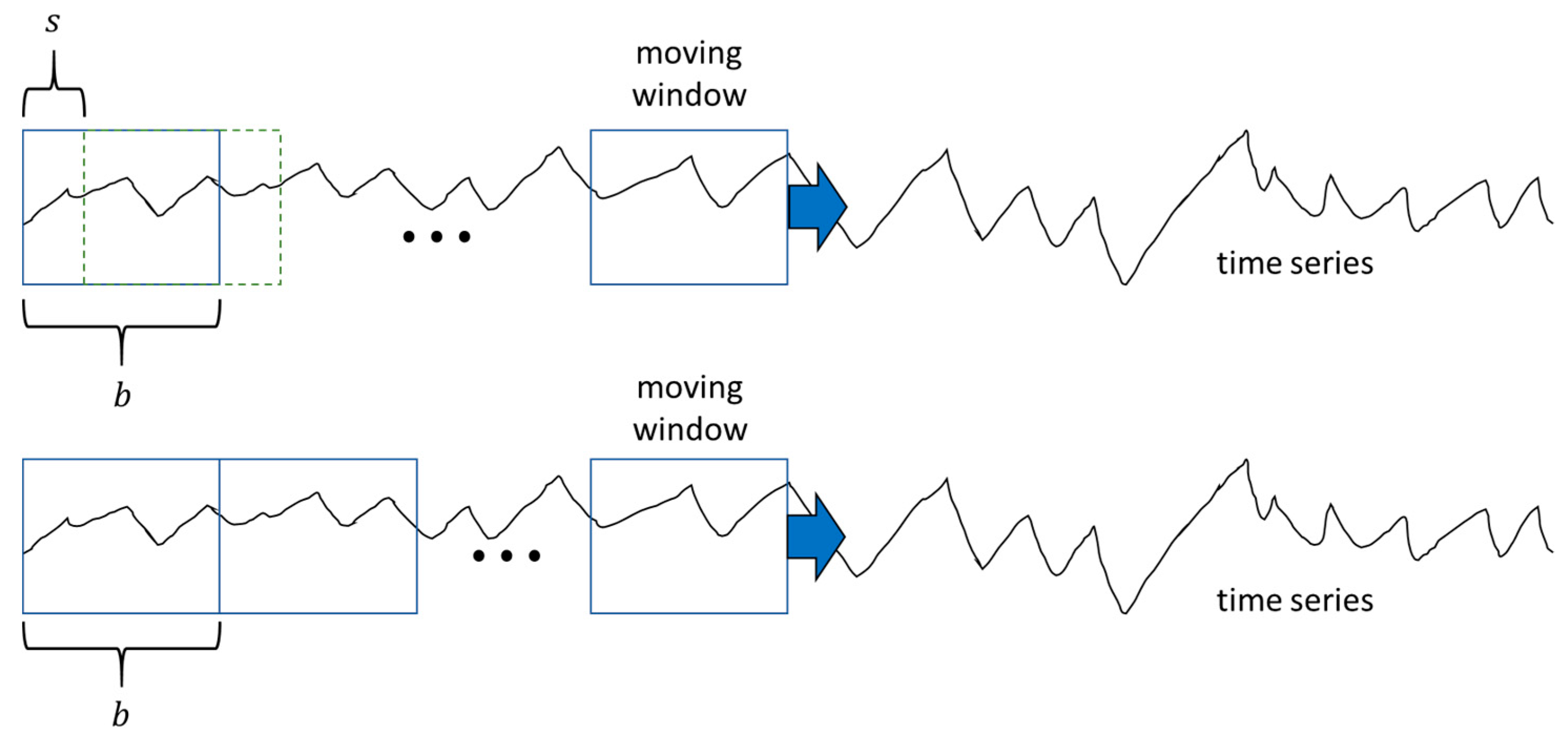
Once the model is constructed, it is implemented online by moving the window of length along the measured time series data with a step size , as indicated in Figure 5. The smaller the values of and , the more rapidly the model will respond to changing conditions, albeit at a higher computational cost. The optimal values of these parameters are system dependent and need to be determined empirically or heuristically by the user on a case-by-case basis, or alternatively by a grid search over a training database.
3. Case Studies
Two cases are considered. In the first case, the controller state of an autogenous mill, as discussed by Aldrich et al. [35], is identified from load measurements only. In the second case study, measurements of temperature and power consumption are used to predict the size distribution of the product of a horizontal stirred mill, as discussed in more detail below.
3.1. Case Study 1: Identification of Controller States in a Fully Autogenous Milling Circuit on a South African Platinum Metal Group Plant
A basic diagram of the milling circuit consisting of a fully autogenous closed-loop mill with a recycling load that overflows from a screen unit is shown in Figure 6. The control variables of the mill, namely, its water inlet, coarse ore feed rate, and fine ore feed rate, are used to control the mill load and the power consumption. The circuit is described in more detail elsewhere [35,36].
Measurements of the mill load were collected approximately every 10 s over a period of almost 89 h of continuous operation. In addition, state labels were logged by the mill controller for each sample collected in the dataset. These logged controller states are related to the operating conditions during the period under investigation, and also reflect the collective, heuristic knowledge of the operation of the comminution circuit. Normal operating conditions were not defined formally, but could be considered as the default state of the mill, i.e., when none of the other conditions were flagged by the controller.
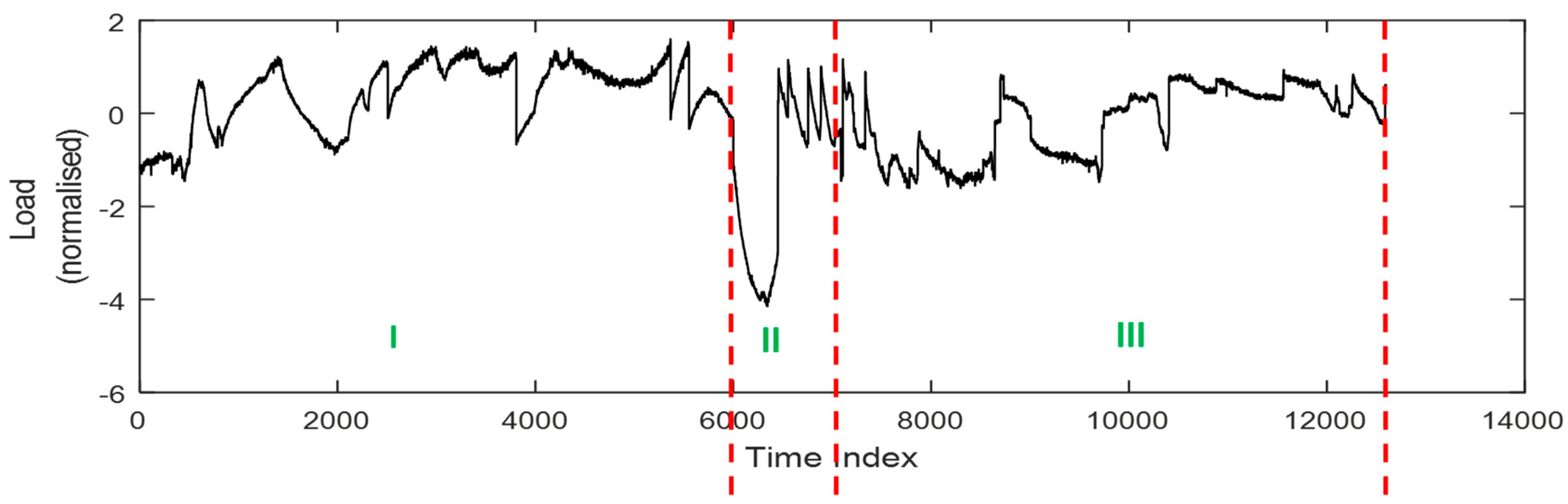
Not all the data logged over the 89 h period were used, as only three of the operational states described by Aldrich et al. [35] were considered. As a result, the mill load data obtained from an autogenous mill contained a total of 12,600 observations from these three operational states, namely, normal operating condition (NOC), feed disturbance (FD), and feed limited (FL), as defined by an expert mill controller [35]. A feed disturbance (FD) is identified when the combined ore feed rate is in excess of the average feed rate by a set threshold. In contrast, a feed limited (FL) state prevails when the mill load shows a rate of change less than zero, while the combined ore feed rate is in excess of the average rate.
As indicated in Figure 7, the NOC (I) and FL states (III) in particular are not easily distinguishable from one other based on a visual inspection of the load measurements of the mill only.
The autocorrelation function (ACF) of the data shown in Figure 7 is shown in Figure 8. The autocorrelation decreases to a negligible value (<0.2) at a lag of approximately 250 and this value was used as the length of the time series segments, i.e., b = 250. Subsequent analyses have indicated that an even smaller value (e.g., b = 125) would still have given satisfactory results, which suggests that the ACF criterion used in this investigation is conservative. This was not investigated in further detail, but more work on this criterion would be required in future studies.
This time series was consequently partitioned into K contiguous segments, each containing b = 250 observations. A breakdown of the partitioning of the time series data of the different mill controller states is given in Table 1. A total of 50 segments, each with a length of 250, were used to calculate the Euclidean distance matrices.
During implementation of the model, the step size was set equal to the window size, s = b, to ensure that each image contained new data only. This was for illustrative purposes only and a lower value for the step size might have been more appropriate if rapid detection of changes in the operating states was the primary objective.
3.2. Case Study 2: Estimation of Product Size in a Horizontal Stirred Mill on an Australian Base Metal Plant
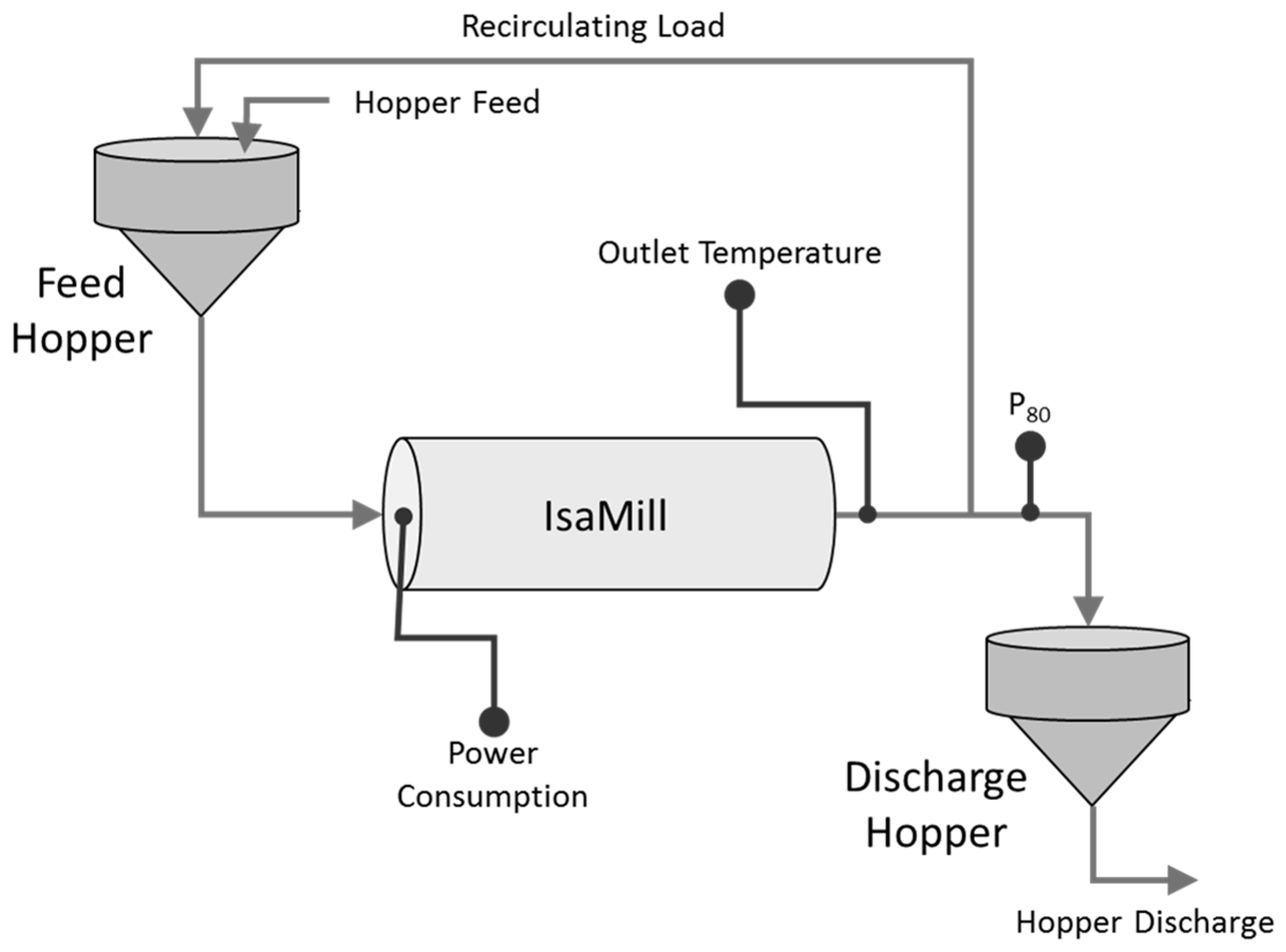
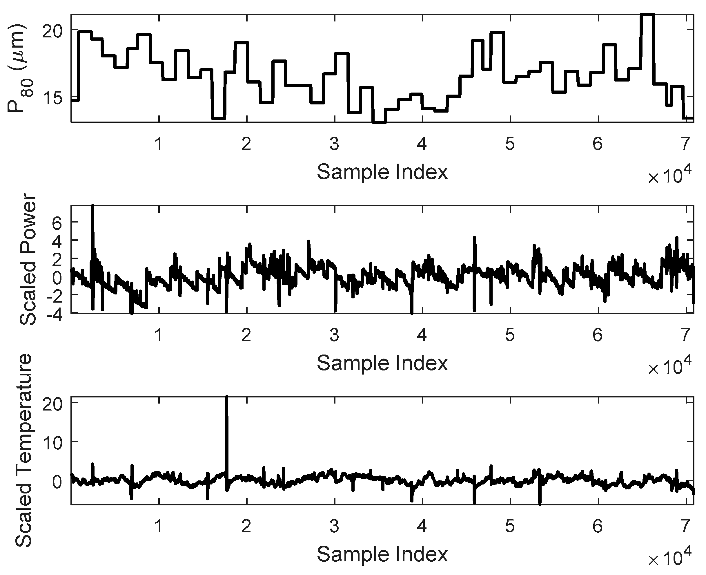
Two variables, namely, power consumption and the temperature, were obtained from a horizontal stirred mill (IsaMill) operating on a base metal plant in Australia. A simplified diagram of the grinding circuit is shown in Figure 9. For proprietary reasons, these variables were scaled to zero mean and unit variance, as shown in Figure 10. The data were obtained from continuous operation of the mill, resulting in a total of 70,842 observations collected over a period of approximately two months.
The product size (P80 values) of the mill was measured off-line once every 24 h and had to be fused with the temperature and power data that were collected every minute. This was done based on a ‘hold until updated’ approach on the same timeline as the power and temperature samples, as indicated in the top panel in Figure 10.
Based on an autocorrelation analysis of the times series variables, both time series were partitioned into segments of length equal to b = 720. These segments were not contiguous, as with the first case study, but were generated with a sliding window with a step size of s = 100. Other values were also tested, but this did not have a material effect on the overall results. As shown in Figure 11 and Table 2, the particle sizes were grouped into three classes, which represent the particle size distribution that could be either fine (Class 1), intermediate (Class 2), or coarse (Class 3).
In this case study, a soft sensor is simulated, designed to predict the particle size class from measurements of the power consumption and temperature of the mill load only. Over a comparatively short period of approximately two months, 50 different P80 values were measured and the data were therefore divided into a training data set containing 40 of the 50 particle sizes (spread across the three classes summarized in Table 2), as well as a test data set containing 10 of the 50 particle sizes. This split in the data was not random, but sequential in time, so as to simulate a soft sensor constructed from data during a given period of data collection and then used to predict (classify the particle size) in a subsequent period.
The soft sensor model was based on the use of a support vector machine to identify the P80 class (1, 2, or 3) based on feature sets extracted from the power, temperature, or measurements of both. Five-fold cross-validation was used to construct the model from the training data set. The test set was not used in the development of the model.
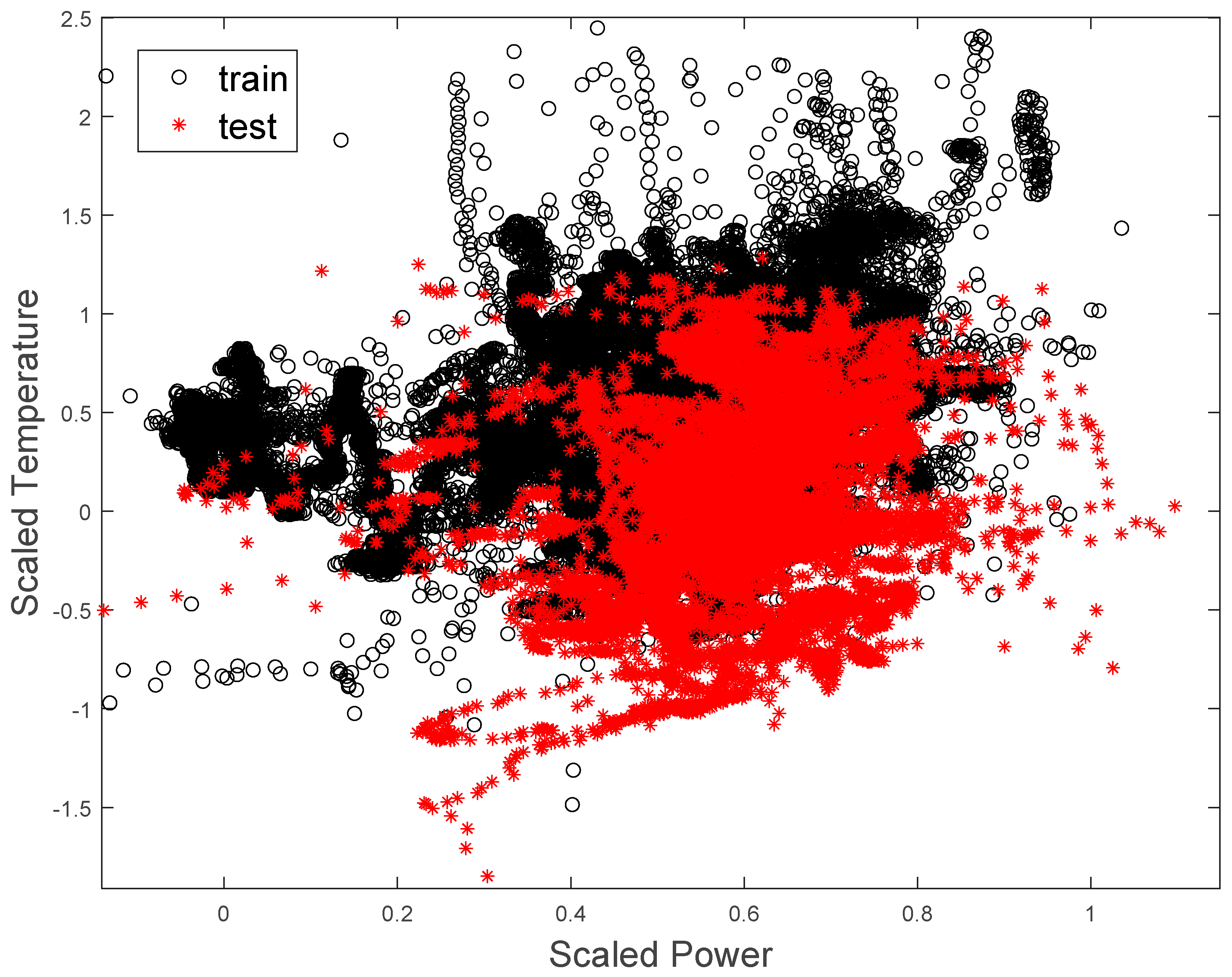
It is important to note that owing to the short period over which data were collected and the variability of plant operation, the training and test data sets had similar, but not identical distributions. This is illustrated in Figure 12, where the incomplete overlap of the training data (black ‘o’) and test data (‘*’) can be seen.
4. Results
4.1. Case Study 1
The time series load data were used to classify the three mill operational states, i.e., normal operating condition, feed disturbance, and feed limited. Representative plots of the distance matrices of each operational state are displayed in Figure 13. In this figure, the colors range from dark blue to bright yellow (Matlab’s default colormap) denoting very small to very large distances. The figures are symmetrical around the diagonals running from the top left to the bottom right of the figures.
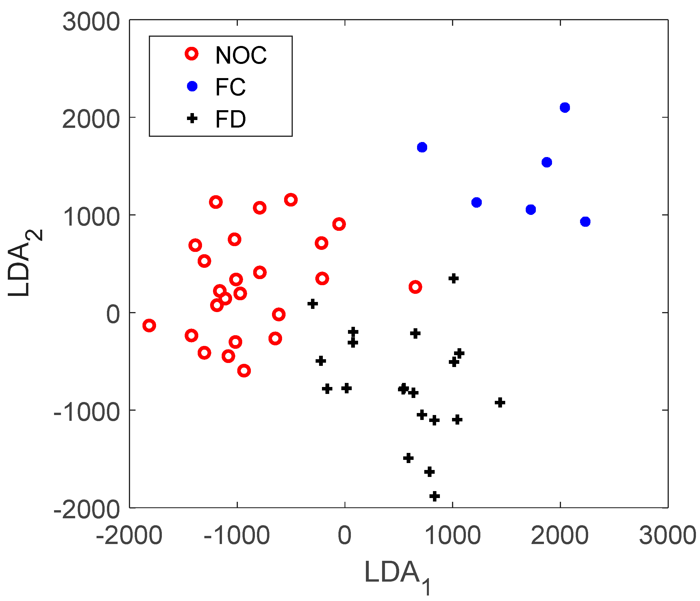
Prior to the classification task, the texton features were visualized by projecting the linear discriminant scores onto 2D space. Virtually complete separation of the three classes can be seen in Figure 14, and it is clear that the control states of the mill can be identified from the mill load only.
This shows that the operational states of the mill can be inferred from load measurements only. Moreover, the models considered here could, in principle, be implemented online once calibrated appropriately and subsequently could form the foundation for more advanced process control models for autogenous mills.
4.2. Case Study 2
Figure 16 shows typical Euclidean distance matrices for each of the three particle size classes derived from the power (top) and temperature (middle) variables. The color map is the same as that used in Figure 13, i.e., small distances are represented by dark blue hues, while large distances are indicated by light green and bright yellow. The bright yellow horizontal and vertical lines in the top and middle panels are indicative of possible outliers in the data, but these were not removed.
The bottom panels in the figure show the Euclidean distance matrices derived from both variables simultaneously, or the cross distances between observations. That is, the distances were determined from , for , where x = power and y = temperature.
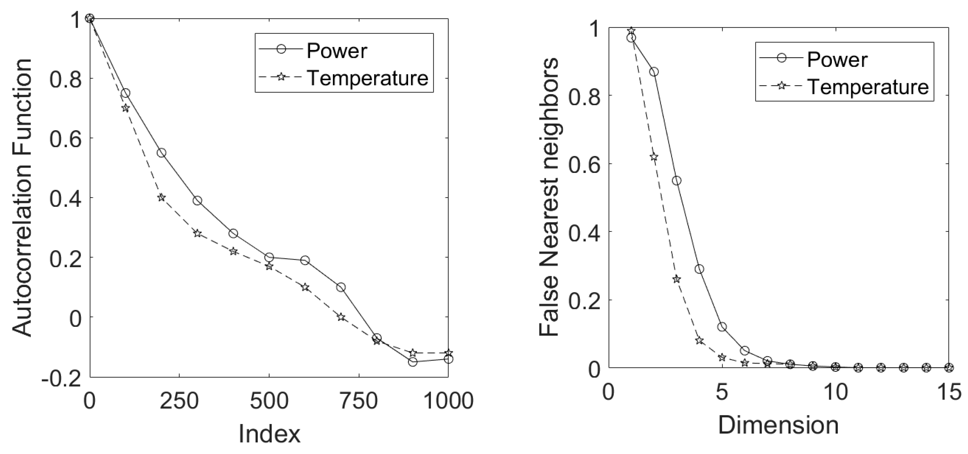
A total of 11 feature sets were extracted from the distance matrices of the power variable the temperature variable ), cross distance matrices of power and temperature variables (), and feature sets derived from the lagged trajectory (LTM) embeddings of the power and temperature variables The embedding parameters and were determined from the autocorrelation functions and by use of the false nearest neighbor algorithm [31], as shown in Figure 17. The above feature matrices were used as predictors in building the classification models.
Since the AlexNet and VGG16 feature sets were comparatively large (4096 features each), the authors also performed dimensionality reduction of these features using principal component analysis, but using the first 20 principal component scores of these large feature sets did not result in better SVM models than when all the features were used.
Five-fold cross-validation was used to partition the data. For each fold, a model was trained using all the data outside the fold, followed by testing using the data inside the fold. The results of using the above features sets to classify the P80 values are shown in Table 3, Table 4, Table 5 and Table 6.
As indicated in these tables, it is not possible to distinguish statistically between the different algorithms based on the average values (% overall reliability of the classifiers), owing to the large standard deviations associated with these values. However, since the folds were not selected randomly from the data, and each fold represents a unique portion of the data set, the classifiers could also be scored on their performance based on the folds, with the winner allotted a score of 1 and all the others zero. On this basis, the algorithms could be ranked as follows (with scores in parentheses): VGG16 (7.5), LTM (5), ALEX (1.5), and TEX (1).
It is interesting that the VGG16 performed significantly better than AlexNet over all feature sets, which is in keeping with other comparative studies between these two algorithms. Also of interest is the fact that the VGG16 algorithm scored higher than the LTM approach often used in the development of dynamic process models. This observation is consistent with the premise that deeper neural networks can lead to better classification models in complex decision spaces [26,28,38].
The reconstructed attractors for both variables can be visualized by plotting the first three dimensions of the trajectory matrix in each case, as shown in Figure 18. These plots are not necessarily able to capture all the variance in the data, but provide some indication of the segregation of the data labels in these phase spaces.
5. Discussion and Conclusions
In this study, analysis of the structures of time series data were investigated based on the Euclidean distance matrices of the observations. More specifically, the elements of these matrices were treated as analogous to the pixels in images, which made them amenable to multivariate image analysis. Three state-of-the-art algorithms were used for this purpose, based on textons, as well as two convolutional neural networks, AlexNet and VGG16, that have recently led to unprecedented improvements in image recognition.
The main parameters that need to be specified by the user are the window size, or length of the time series segment on which the distance matrix calculations are based, and the step size with which this window is moved along the time series. Some guidelines were given with regard to the selection of the window size, based on analysis of the autocorrelation function of the time series data. Alternatively, both parameters generally would need to be optimized empirically, as their optimal values would be system dependent.
The methodology was applied to two case studies associated with comminution systems in the mineral processing industries and was used to capture the dynamic behavior of a few key variables in these systems. By using features extracted with the above algorithms as predictors, classification models could be constructed to identify mill control states and mill particle sizes.
The following conclusions can be made from the results.
- Of the three algorithms, the VGG16 convolutional neural network appeared to yield the best performance overall.
- The controller states of a fully autogenous mill could be identified with a high degree of accuracy with the proposed methodology—significantly more so than was possible with a conventional approach using lagged variables as predictors.
- The general approach also compared favorably with a traditional approach in the identification of product size in a horizontal stirred mill, although only marginally so. Although the particle sizes could not be identified with a high degree of accuracy in this case, the models could likely be improved substantially with the availability of more plant data.
Finally, it should be noted that the methodology could be used for time series analysis in general, including forecasting, classification, and clustering, and this should be confirmed by further investigation on larger and more general data sets and systems.
Acknowledgments
J.P.B. is grateful for financial support from the Western Australian School of Mines.
Author Contributions
Chris Aldrich conceptualized the study and designed the experiments. He and Jason Bardinas developed the algorithms and implemented them computationally. Lara Napier acquired, collected and analyzed the data in the second case study. Chris Aldrich and Jason Bardinas co-wrote the paper.
Conflicts of Interest
The authors declare no conflict of interest.
References
- Fuerstenau, D.W.; Abouzeid, A.-Z.M. The energy efficiency of ball milling in comminution. Int. J. Miner. Process. 2002, 67, 161–185. [Google Scholar] [CrossRef]
- Aguila-Camacho, N.; le Roux, J.D.; Duarte-Mermpud, M.A.; Orchard, M.E. Control of a grinding mill circuit using fractional order controllers. J. Process Control 2017, 53, 80–94. [Google Scholar] [CrossRef]
- Zeng, Y.; Forssberg, K.S.E. Application of vibration signals to monitoring crushing parameters. Powder Technol. 1993, 76, 247–252. [Google Scholar] [CrossRef]
- Zeng, Y.; Forssberg, K.S.E. Monitoring grinding parameters by vibration signal measurement—A primary application. Miner. Eng. 1994, 7, 495–501. [Google Scholar] [CrossRef]
- Zeng, Y.; Forssberg, K.S.E. Vibration signal emission from mono-size particle breakage. Int. J. Miner. Process. 1996, 44–45, 59–69. [Google Scholar] [CrossRef]
- Theron, D.A.; Aldrich, C. Acoustic estimation of the particle size distributions of sulphide ores in a laboratory ball mill. J. S. Afr. Inst. Min. Metall. 2000, 100, 243–248. [Google Scholar]
- Tang, J.; Chai, T.; Yu, W.; Zhao, L. Feature extraction and selection based on vibration spectrum with application to estimating the load parameters of ball mill in grinding process. Control Eng. Pract. 2012, 20, 991–1004. [Google Scholar] [CrossRef]
- Liu, Z.; Chai, T.; Yu, W.; Tang, J. Multi-frequency signal modeling using empirical mode decomposition and PCA with application to mill load estimation. Neurocomputing 2015, 169, 392–402. [Google Scholar] [CrossRef]
- Tang, J.; Zhao, L.-J.; Zhou, J.-W.; Yiue, H.; Chai, T.-Y. Experimental analysis of wet mill load based on vibration signals of laboratory-scale mill shell. Miner. Eng. 2010, 23, 720–730. [Google Scholar] [CrossRef]
- Li, Y.; Shao, C. Application of grey relation analysis and RBF network on grinding concentration’s soft sensing. IFAC Proceed. Vol. 2005, 38, 74–79. [Google Scholar]
- Aldrich, C.; Auret, L. Unsupervised Process Monitoring and Fault Diagnosis with Machine Learning Methods; Series: Advances in Pattern Recognition; Springer: London, UK, 2013; p. 374. ISBN 978-1-4471-5184-5. [Google Scholar]
- Aghabozorgi, S.; Seyed Shirkhorshidi, A.; Ying Wah, T. Time series clustering—A decade review. Inf. Syst. 2015, 53, 16–38. [Google Scholar] [CrossRef]
- Julesz, B. Textons, the elements of texture perception, and their interaction. Nature 1981, 290, 91–97. [Google Scholar] [CrossRef] [PubMed]
- Julesz, B. A brief outline of the texton theory of human vision. Trends Neurosci. 1984, 7, 41–45. [Google Scholar] [CrossRef]
- Kistner, M.; Jemwa, G.T.; Aldrich, C. Monitoring of mineral processing systems by using textural image analysis. Miner. Eng. 2013, 52, 169–177. [Google Scholar] [CrossRef]
- Leung, T.; Malik, J. Representing and recognizing the visual appearance of materials using three-dimensional textons. Int. J. Comput. Vis. 2001, 43, 29–44. [Google Scholar] [CrossRef]
- Jemwa, G.T.; Aldrich, C. Estimating size fraction categories of coal particles on conveyor belts using image texture modeling methods. Expert Syst. Appl. 2012, 39, 7947–7960. [Google Scholar] [CrossRef]
- Varma, M.; Zisserman, A. A statistical approach to texture classification from single images. Int. J. Comput. Vis. 2005, 62, 61–81. [Google Scholar] [CrossRef]
- Schmid, C. Constructing models for content-based image retrieval. In Proceedings of the IEEE Computer Society Conference on Computer Vision and Pattern Recognition, Kauai, HI, USA, 8–14 December 2001. [Google Scholar]
- Krizhevsky, A.; Sutskever, I.; Hinton, G.E. Imagenet classification with deep convolutional neural networks. Neural Inf. Process. Syst. 2012, 1097–1105. [Google Scholar] [CrossRef]
- Fu, Y.; Aldrich, C. Froth image analysis by use of transfer learning and convolutonal neural networks. Miner. Eng. 2018, 115, 68–78. [Google Scholar] [CrossRef]
- Sharma, H.; Zerbe, N.; Klempert, I.; Hellwich, O.; Hufnagl, P. Deep neural networks for automatic classification of gastric carcinoma using whole-slide images in digital histopathology. Comput. Med. Imaging Gr. 2017, 61, 2–13. [Google Scholar] [CrossRef] [PubMed]
- Isin, A.; Ozdalili, S. Cardiac arrhythmia detection using deep learning. Procedia Comput. Sci. 2017, 120, 268–275. [Google Scholar] [CrossRef]
- Boddapati, V.; Petef, A.; Rasmussen, J.; Lundberg, L. Classifying environmental sounds using image recognition networks. Procedia Comput. Sci. 2017, 112, 2048–2056. [Google Scholar] [CrossRef]
- Capobianco, S.; Marinai, S. Deep neural networks for record counting in historical handwritten records. Pattern Recognit. Lett. 2017. [Google Scholar] [CrossRef]
- Ghazi, M.M.; Yanikoglu, B.; Aptoula, E. Plant identification using deep neural networks via optimization of transfer learning parameters. Neurocomputing 2017, 235, 228–235. [Google Scholar] [CrossRef]
- Nogueira, K.; Penatti, O.A.B.; dos Santos, J.A. Towards better exploiting convolutional neural networks for remote sensing scene classifcation. Pattern Recognit. 2017, 61, 539–556. [Google Scholar] [CrossRef]
- Simonyan, K.; Zisserman, A. Very deep convolutional networks for large-scale image recognition. arXiv, 2014; arXiv:1409.1556. [Google Scholar]
- Ma, S.; Bargal, S.A.; Zhang, J.; Sigal, L.; Scalroff, S. Do less and achieve more: Training CNNs for action recognition utilizing action images from the Web. Pattern Recognit. 2017, 68, 334–345. [Google Scholar] [CrossRef]
- Jozwik, K.M.; Kriegeskorte, M.; Storrs, K.R.; Mur, M. Deep convolutional neural networks outperform feature-based but not categorical models in explaining object similarity judgments. Front. Psychol. 2017, 8, 1726. [Google Scholar] [CrossRef] [PubMed]
- Barnard, J.P.; Aldrich, C.; Gerber, M. Identification of dynamic process systems with surrogate data methods. AIChE J. 2001, 47, 2064–2075. [Google Scholar] [CrossRef]
- Fabretti, A.; Ausloos, M. Recurrence plot and recurrence quantification analysis techniques for detecting a critical regime. Ex. Financ. Mark. Indices 2004. [Google Scholar] [CrossRef]
- Kim, S.; Choi, Y.; Lee, M. Deep learning with support vector data description. Neurocomputing 2015, 165, 111–117. [Google Scholar] [CrossRef]
- Tax, D.M.J.; Duin, R.P.W. Support vector data description. Mach. Learn. 2004, 54, 45–66. [Google Scholar] [CrossRef]
- Aldrich, C.; Burchell, J.J.; Groenewald, J.W.d.V.; Yzelle, C. Visualization of the controller states of an autogenous mill from time series data. Miner. Eng. 2014, 56, 1–9. [Google Scholar] [CrossRef]
- Burchell, J.J.; Aldrich, C.; Groenewald, J.W.d.V.; Barnard, J.P. Tracking the operational states of an autogenous mill on a concentrator plant. In Proceedings of the South African Chemical Engineering Congress, Cape Town, Western Cape, South Africa, 20–22 September 2009. [Google Scholar]
- Aldrich, C.; Napier, L.F.A. Development of soft sensors for stirred mill grinding circuits based on random forest and principal component models. In Proceedings of the 17th IFAC World Congress, Toulouse, France, 9–14 July 2017. [Google Scholar]
- Yu, W.; Yang, K.; Bai, Y.; Xiao, T.; Yao, H.; Rui, Y. Visualizing and comparing AlexNet and VGG using deconvolutional layers. In Proceedings of the 33rd International Congress on Machine Learning, New York, NY, USA, 19–24 June 2016; JMLR W & CP. Volume 48. [Google Scholar]
Figure 1.
Schematic workflow of the study, comprising the time series data (A), segmentation of the data (B), calculation of distance matrix for each time series segment (C), and extraction of texture features from each matrix (D) from which models can be built to relate the features to the descriptive labels associated with the time series data.
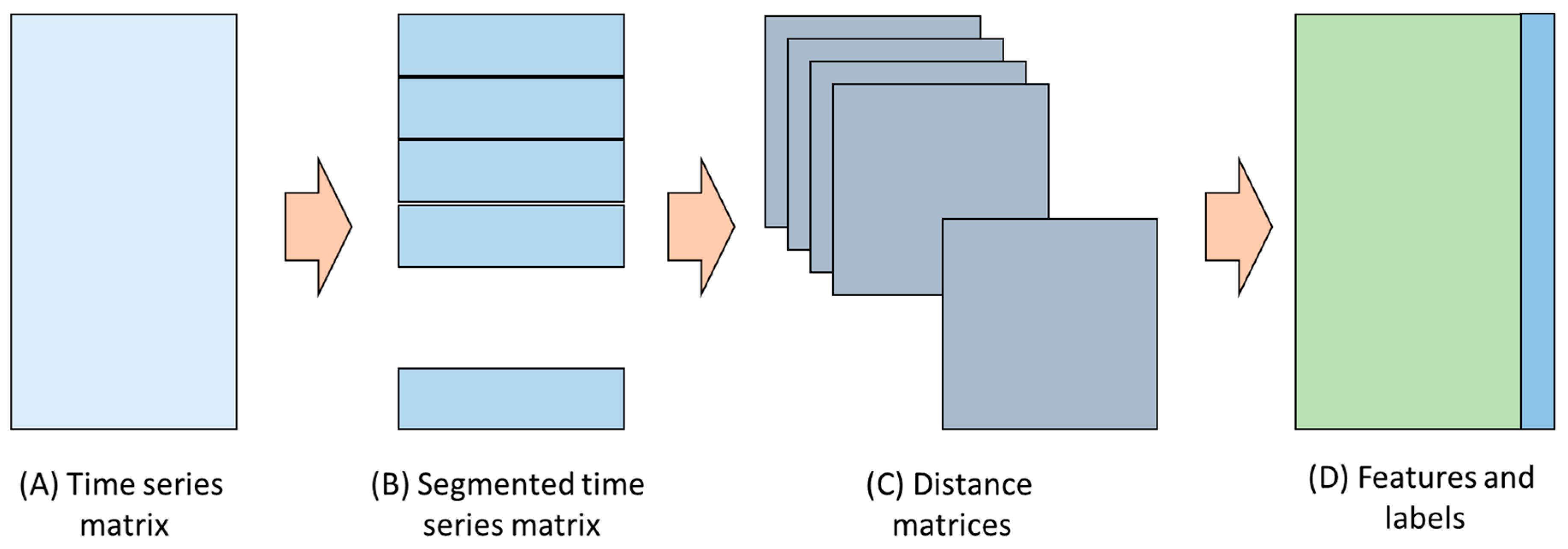
Figure 2.
Convolution of a 4 × 4 image () with a 3 × 3 filter (), yielding 4 features ().
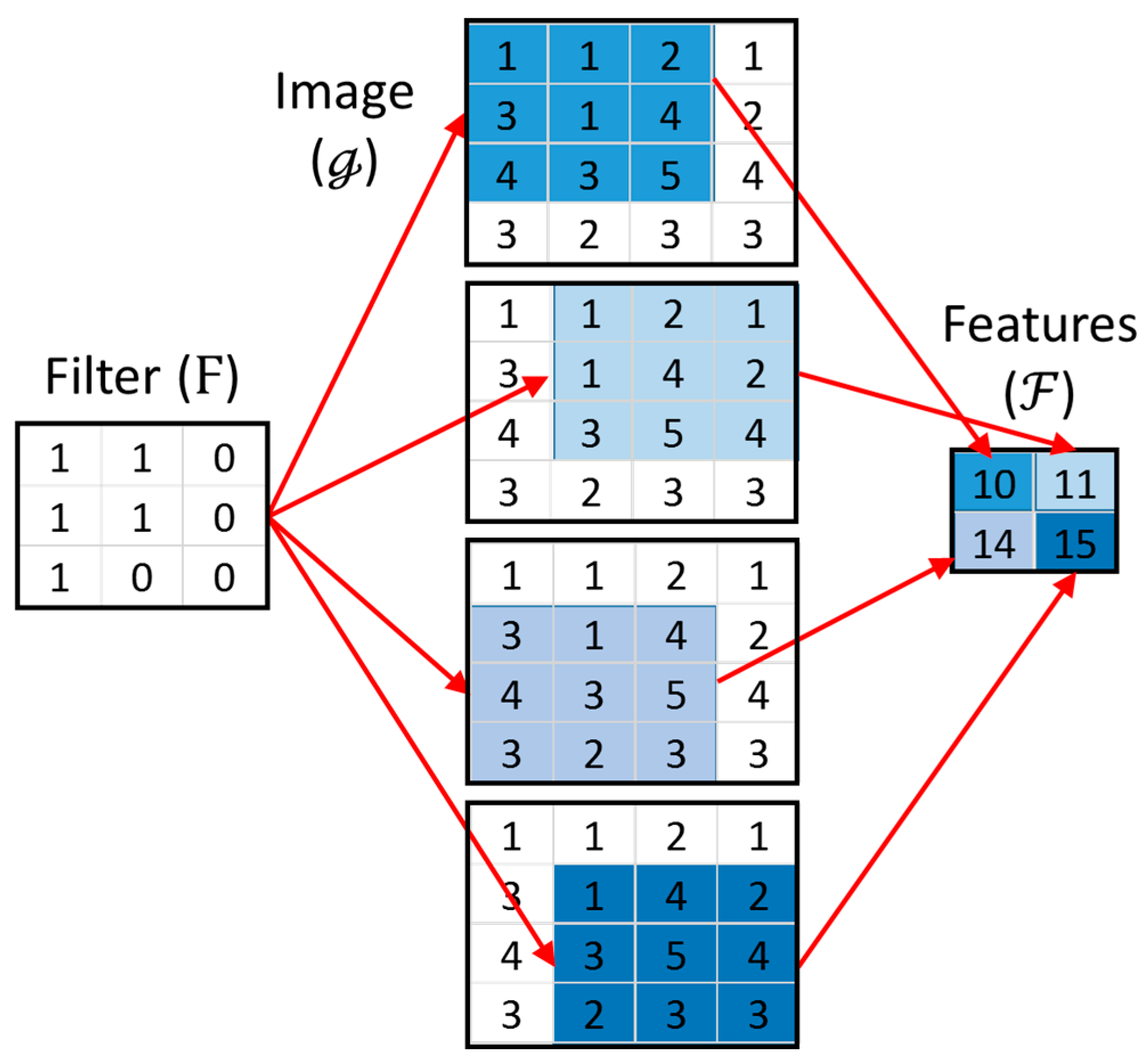
Figure 3.
A simplified version of the architecture of AlexNet showing convolutional (Conv), pooling (Pool), and fully connected (FC) layers.
Figure 3.
A simplified version of the architecture of AlexNet showing convolutional (Conv), pooling (Pool), and fully connected (FC) layers.
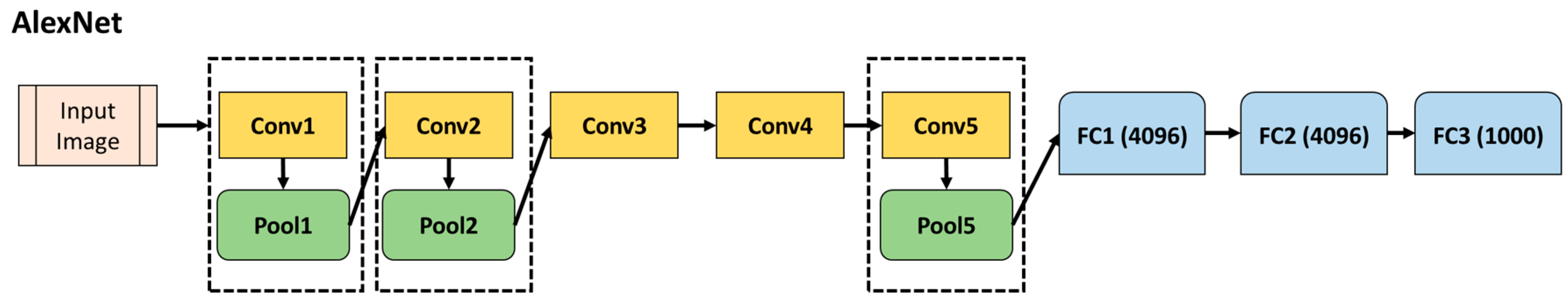
Figure 4.
A simplified version of the architecture of VGG16 neural network showing the different convolutional (Conv), pooling (Pool), and fully connected (FC) layers.
Figure 4.
A simplified version of the architecture of VGG16 neural network showing the different convolutional (Conv), pooling (Pool), and fully connected (FC) layers.
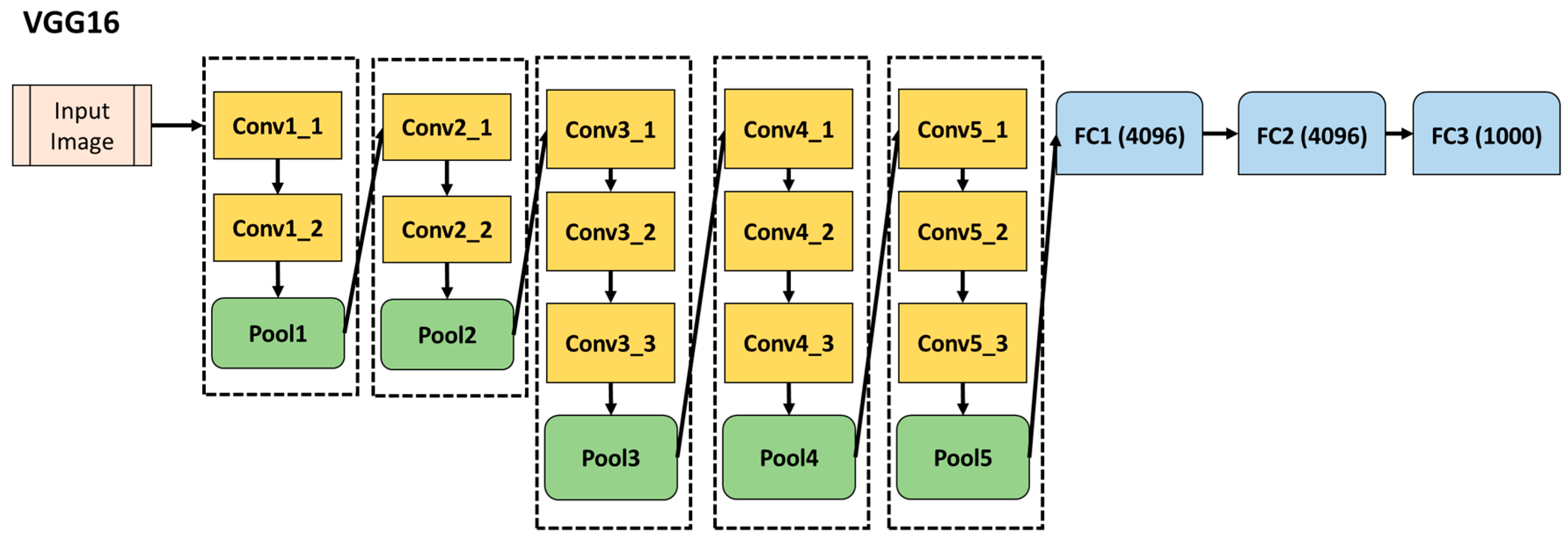
Figure 5.
Online application of the model, whereby a window of length is moved along the time series with a step size (top) and (bottom).
Figure 5.
Online application of the model, whereby a window of length is moved along the time series with a step size (top) and (bottom).

Figure 6.
Basic diagram of fully autogenous grinding circuit (after Aldrich et al. [35]).
Figure 6.
Basic diagram of fully autogenous grinding circuit (after Aldrich et al. [35]).
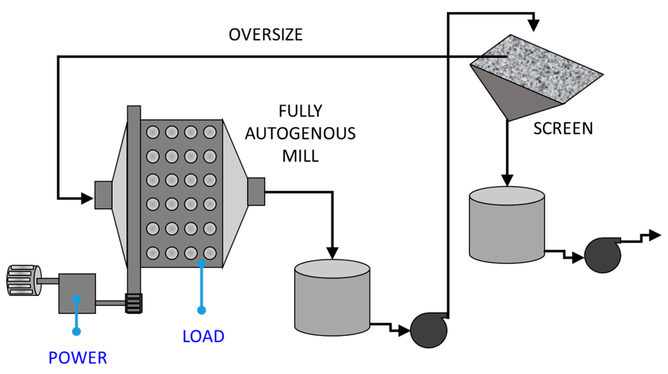
Figure 7.
The normalized mill load with labelled states: (I) normal operating condition (NOC), (II) Feed disturbance, (III) Feed limited.
Figure 7.
The normalized mill load with labelled states: (I) normal operating condition (NOC), (II) Feed disturbance, (III) Feed limited.

Figure 8.
The autocorrelation function (ACF) of the mill load time series showing a low to negligible value at an index exceeding a window length of b = 250.
Figure 8.
The autocorrelation function (ACF) of the mill load time series showing a low to negligible value at an index exceeding a window length of b = 250.
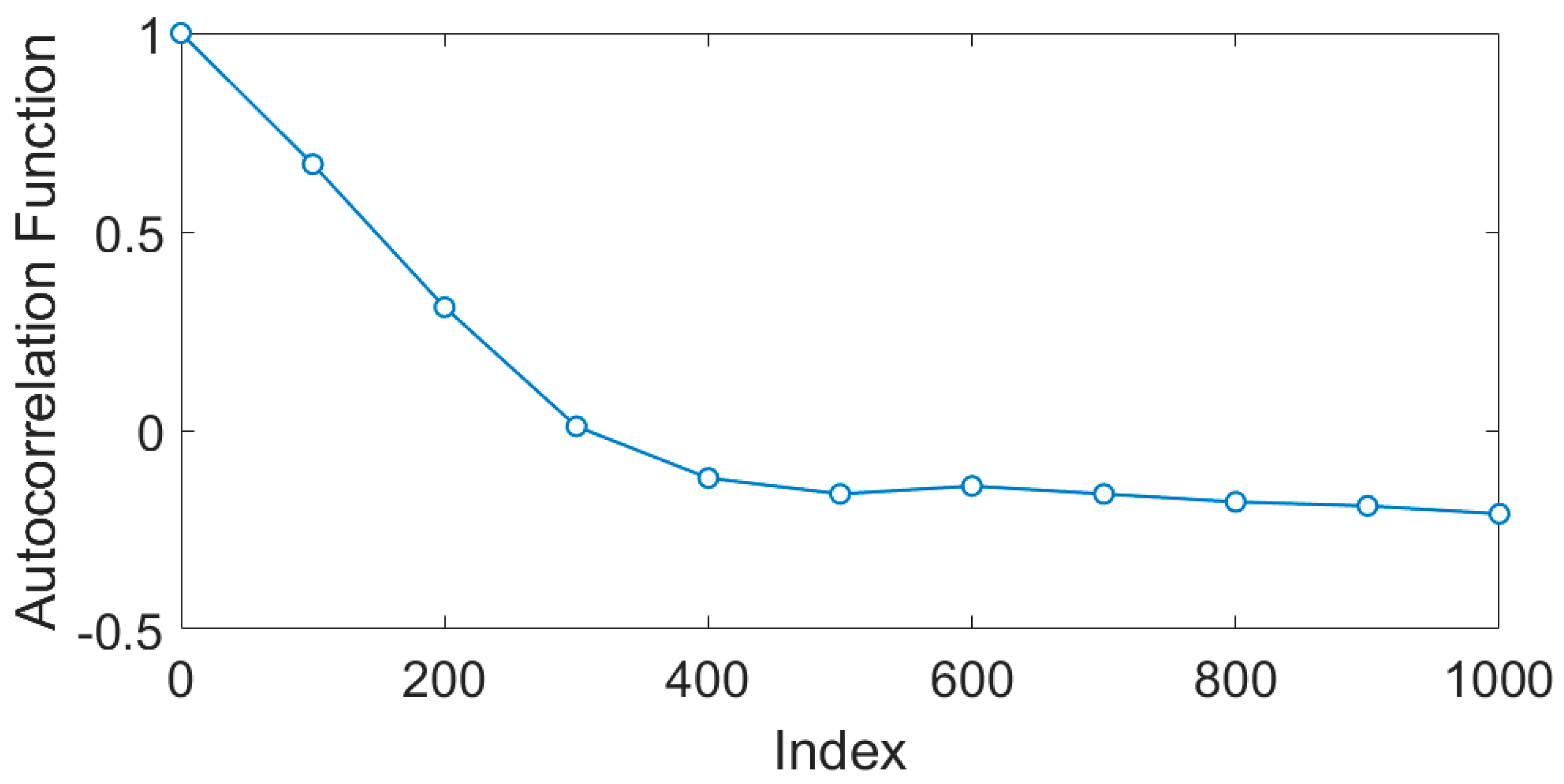
Figure 9.
Flow diagram of the IsaMill grinding circuit, showing the measuring points of the power, temperature, and P80 particle size (after Aldrich and Napier [37]).
Figure 9.
Flow diagram of the IsaMill grinding circuit, showing the measuring points of the power, temperature, and P80 particle size (after Aldrich and Napier [37]).

Figure 10.
The raw time series of P80 particle size (top), scaled power consumption (middle), and scaled temperature (bottom) of the IsaMill mill.
Figure 10.
The raw time series of P80 particle size (top), scaled power consumption (middle), and scaled temperature (bottom) of the IsaMill mill.

Figure 11.
Distribution of particle size classes as a function of scaled temperature and power measurements.
Figure 11.
Distribution of particle size classes as a function of scaled temperature and power measurements.
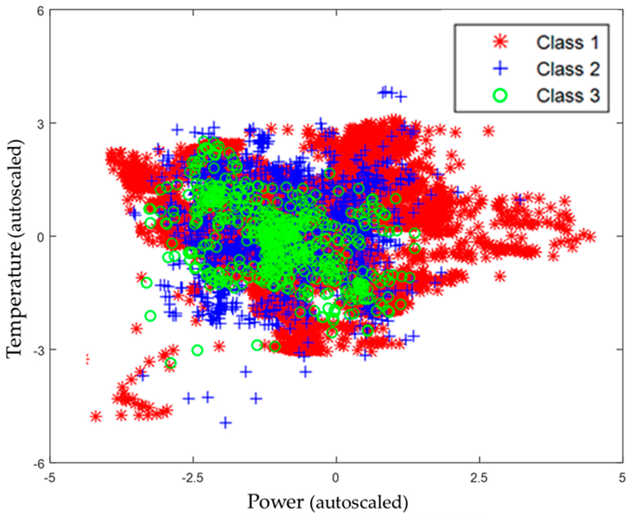
Figure 12.
Distribution of training (black ‘o’) and test (red ‘*’) data sets.

Figure 13.
Representative plot of the Euclidean distance matrices of three control states of the autogenous mill, i.e., normal operating conditions (left), feed disturbance (middle) and a feed limited state (right). Small values are indicated by dark blue colors on the one extreme, while large distance values are indicated by bright yellow colors.
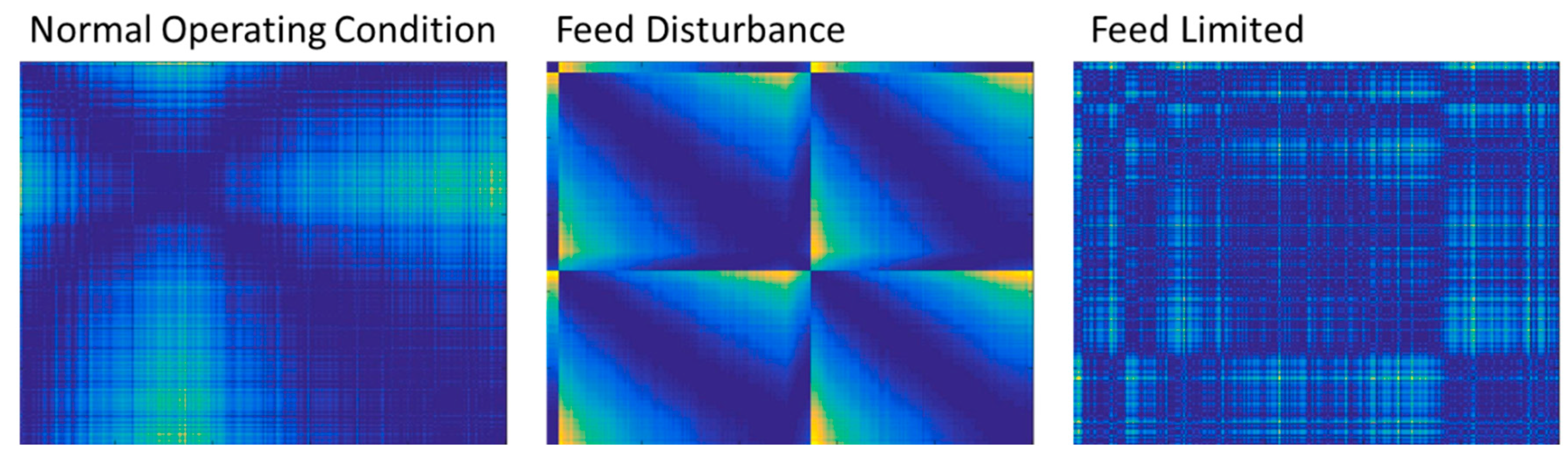
Figure 14.
Visualization of the texton feature set of the mill load data (Case Study 1) as projected onto 2D space using linear discriminant scores, LDA1 and LDA2.
Figure 14.
Visualization of the texton feature set of the mill load data (Case Study 1) as projected onto 2D space using linear discriminant scores, LDA1 and LDA2.

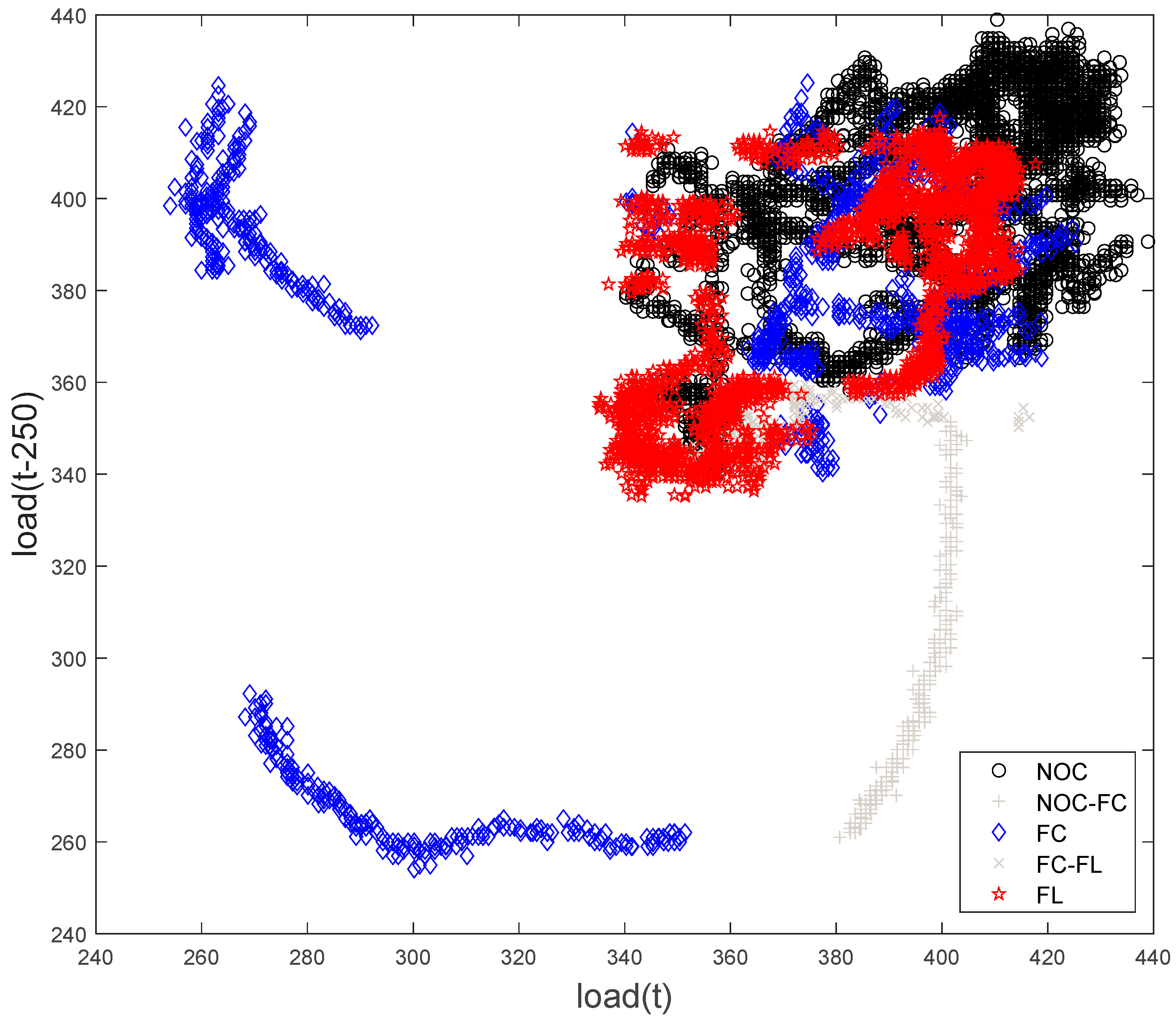
Figure 15.
Visualization of the LTM feature set of the mill load data (Case Study 1), showing the NOC, FC, and FL control states. The scores indicated by ‘NOC–FC’ and ‘FC–FL’ show transitions between the NOC and FC and FC and FL states, respectively.
Figure 15.
Visualization of the LTM feature set of the mill load data (Case Study 1), showing the NOC, FC, and FL control states. The scores indicated by ‘NOC–FC’ and ‘FC–FL’ show transitions between the NOC and FC and FC and FL states, respectively.

Figure 16.
Distance matrix plots of 3 classes—fine (left), intermediate (middle), and coarse (right)—using time series of power draw (top), outlet temperature (middle), and cross distance of these variables (bottom). Small values are indicated by dark blue colors on the one extreme, while large distance values are indicated by bright yellow colors.
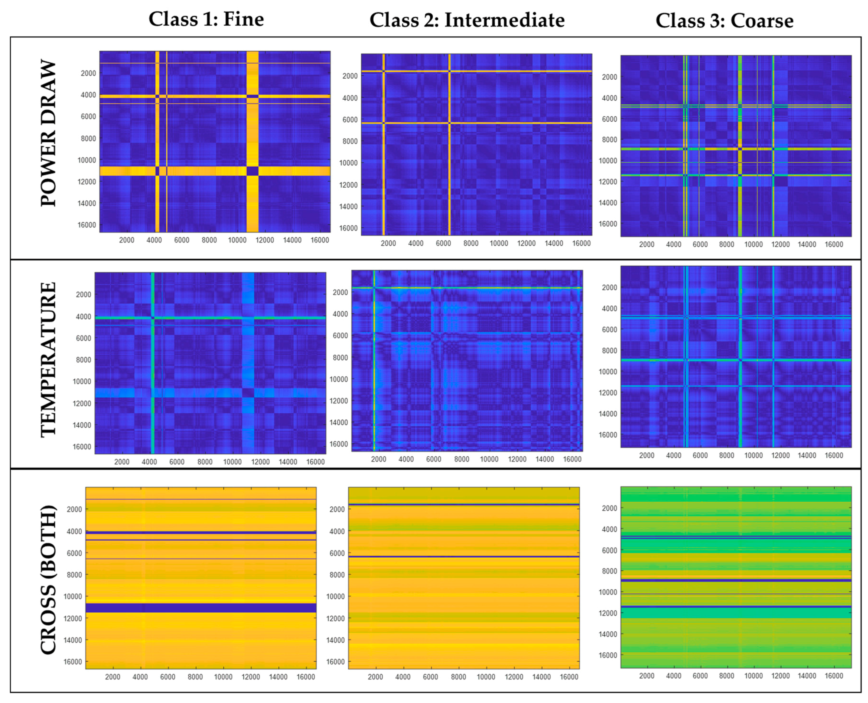
Figure 17.
The autocorrelation function (left) and false nearest neighbor (right) plots of power draw (solid lines) and outlet temperature (broken lines) time series.
Figure 17.
The autocorrelation function (left) and false nearest neighbor (right) plots of power draw (solid lines) and outlet temperature (broken lines) time series.

Figure 18.
The reconstructed attractors of power draw (left) and outlet temperature (right) time series data with legend: fine (red ‘*’), intermediate (blue ‘+’), and coarse (green ‘o’).
Figure 18.
The reconstructed attractors of power draw (left) and outlet temperature (right) time series data with legend: fine (red ‘*’), intermediate (blue ‘+’), and coarse (green ‘o’).


Table 1.
Mill load measurements and number of time series segments for b = 250.
| Mill States | Number of Observations | Number of Segments |
|---|---|---|
| Normal Operating Condition (NOC) | 6000 | 24 |
| Feed Disturbance (FD) | 1500 | 6 |
| Feed Limited (FL) | 5100 | 20 |
| 12,600 | 50 |
Table 2.
Distribution of P80 particle size classes in the IsaMill.
| Particle Size (μm) | Class | Description | No of Observations | No of Segments * |
|---|---|---|---|---|
| 13 P80 < 15 | 1 | Fine (F) | 16,712 | 160 |
| 15 P80 < 18 | 2 | Intermediate (I) | 40,330 | 397 |
| P80 18 | 3 | Coarse (C) | 17,280 | 166 |
| 74,312 | 723 |
* Segments generated with a sliding window of length b = 720 and a step size s = 100.
Table 3.
Results of classification (% correct) with predictor sets derived from the mill power data and use of a cubic kernel support vector machine.
Table 3.
Results of classification (% correct) with predictor sets derived from the mill power data and use of a cubic kernel support vector machine.
| Run | Power | |||||||
|---|---|---|---|---|---|---|---|---|
| TEXTONS | ALEXNET | VGG16 | LTM | |||||
| Train | Test | Train | Test | Train | Test | Train | Test | |
| 1 | 83.3 | 60.0 | 71.3 | 62.7 | 76.6 | 63.4 | 59.5 | 60.9 |
| 2 | 86.5 | 41.9 | 76.7 | 47.3 | 77.9 | 46.5 | 65.5 | 37.1 |
| 3 | 85.0 | 44.7 | 74.2 | 57.5 | 78.3 | 48.1 | 62.7 | 53.6 |
| 4 | 83.7 | 64.9 | 71.6 | 65.0 | 73.6 | 66.4 | 65.4 | 55.3 |
| 5 | 84.3 | 54.2 | 72.0 | 58.8 | 78.1 | 62.6 | 62.9 | 54.6 |
| AVG | 84.6 | 53.1 | 73.2 | 56.3 | 76.9 | 57.4 | 63.2 | 52.3 |
| STD | 1.26 | 9.80 | 2.28 | 8.39 | 1.96 | 9.35 | 2.46 | 8.96 |
Table 4.
Results of classification (% correct) with predictor sets derived from the mill temperature data and use of a cubic kernel support vector machine.
Table 4.
Results of classification (% correct) with predictor sets derived from the mill temperature data and use of a cubic kernel support vector machine.
| Run | Temperature | |||||||
|---|---|---|---|---|---|---|---|---|
| TEXTONS | ALEXNET | VGG16 | LTM | |||||
| Train | Test | Train | Test | Train | Test | Train | Test | |
| 1 | 79.1 | 57.0 | 72.1 | 59.2 | 75.6 | 59.9 | 66.3 | 68.9 |
| 2 | 84.6 | 36.6 | 75.5 | 46.5 | 77.9 | 47.3 | 69.6 | 55.4 |
| 3 | 79.5 | 48.8 | 73.9 | 47.3 | 76.3 | 49.6 | 70.8 | 58.3 |
| 4 | 80.3 | 58.0 | 78.6 | 58.0 | 75.9 | 62.6 | 71.3 | 61.1 |
| 5 | 79.1 | 63.4 | 74.8 | 60.3 | 76.0 | 64.1 | 68.5 | 63.5 |
| AVG | 80.5 | 52.8 | 75.0 | 54.3 | 76.3 | 56.7 | 69.3 | 61.4 |
| STD | 2.33 | 10.43 | 2.39 | 6.77 | 0.91 | 7.72 | 2.00 | 5.16 |
Table 5.
Results of classification (% correct) with predictor sets derived from the cross recurrence combination of mill temperature and power data and use of a cubic kernel support vector machine.
Table 5.
Results of classification (% correct) with predictor sets derived from the cross recurrence combination of mill temperature and power data and use of a cubic kernel support vector machine.
| Run | Cross | |||||||
|---|---|---|---|---|---|---|---|---|
| TEXTONS | ALEXNET | VGG16 | LTM | |||||
| Train | Test | Train | Test | Train | Test | Train | Test | |
| 1 | 69.9 | 59.2 | 59.0 | 57.8 | 69.2 | 63.1 | NA | NA |
| 2 | 76.4 | 50.3 | 65.2 | 45.0 | 74.2 | 46.5 | NA | NA |
| 3 | 74.6 | 46.5 | 67.1 | 46.5 | 74.6 | 48.0 | NA | NA |
| 4 | 72.8 | 64.1 | 59.8 | 67.9 | 73.1 | 66.4 | NA | NA |
| 5 | 72.4 | 58.8 | 63.0 | 61.8 | 72.2 | 60.3 | NA | NA |
| AVG | 73.2 | 55.8 | 62.8 | 55.8 | 72.7 | 56.9 | NA | NA |
| STD | 2.44 | 7.18 | 3.45 | 9.87 | 2.15 | 9.05 | NA | NA |
Table 6.
Results of classification (% correct) with predictor sets derived from combination of the mill temperature and power data and use of a cubic kernel support vector machine.
Table 6.
Results of classification (% correct) with predictor sets derived from combination of the mill temperature and power data and use of a cubic kernel support vector machine.
| Run | Combined Power and Temperature | |||||||
|---|---|---|---|---|---|---|---|---|
| TEXTONS | ALEXNET | VGG16 | LTM | |||||
| Train | Test | Train | Test | Train | Test | Train | Test | |
| 1 | 86.1 | 78.9 | 80.9 | 77.5 | 85.2 | 78.2 | 60.5 | 61.3 |
| 2 | 89.7 | 45.0 | 80.6 | 47.3 | 86.3 | 47.3 | 77.4 | 41.9 |
| 3 | 91.1 | 43.1 | 80.4 | 51.9 | 85.7 | 52.6 | 75.3 | 55.9 |
| 4 | 89.0 | 65.0 | 80.7 | 59.8 | 83.4 | 66.4 | 72.6 | 61.2 |
| 5 | 88.8 | 74.1 | 78.9 | 69.2 | 86.2 | 71.8 | 73.4 | 51.2 |
| AVG | 88.9 | 61.2 | 80.3 | 61.1 | 85.4 | 63.3 | 71.8 | 54.3 |
| STD | 1.83 | 16.5 | 0.80 | 12.4 | 1.18 | 13.0 | 6.60 | 8.10 |
© 2018 by the authors. Licensee MDPI, Basel, Switzerland. This article is an open access article distributed under the terms and conditions of the Creative Commons Attribution (CC BY) license (http://creativecommons.org/licenses/by/4.0/).
Share and Cite
MDPI and ACS Style
Bardinas, J.P.; Aldrich, C.; Napier, L.F.A. Predicting the Operating States of Grinding Circuits by Use of Recurrence Texture Analysis of Time Series Data. Processes 2018, 6, 17. https://doi.org/10.3390/pr6020017
AMA Style
Bardinas JP, Aldrich C, Napier LFA. Predicting the Operating States of Grinding Circuits by Use of Recurrence Texture Analysis of Time Series Data. Processes. 2018; 6(2):17. https://doi.org/10.3390/pr6020017
Chicago/Turabian StyleBardinas, Jason P., Chris Aldrich, and Lara F. A. Napier. 2018. "Predicting the Operating States of Grinding Circuits by Use of Recurrence Texture Analysis of Time Series Data" Processes 6, no. 2: 17. https://doi.org/10.3390/pr6020017
Note that from the first issue of 2016, this journal uses article numbers instead of page numbers. See further details here.