FluxVisualizer, a Software to Visualize Fluxes through Metabolic Networks


1
Institute for Quantitative and Theoretical Biology, Heinrich-Heine-University, 40225 Duesseldorf, Germany
2
IBGC-CNRS UMR 5095, 1 rue Camille Saint Saens, CS 61390, 33077 Bordeaux-cedex, France
3
University of Bordeaux France, 33076 Bordeaux-cedex, France
*
Author to whom correspondence should be addressed.
Processes 2018, 6(5), 39; https://doi.org/10.3390/pr6050039
Submission received: 2 March 2018
/
Revised: 10 April 2018
/
Accepted: 17 April 2018
/
Published: 24 April 2018
(This article belongs to the Special Issue Methods in Computational Biology)
Abstract
:FluxVisualizer (Version 1.0, 2017, freely available at https://fluxvisualizer.ibgc.cnrs.fr) is a software to visualize fluxes values on a scalable vector graphic (SVG) representation of a metabolic network by colouring or increasing the width of reaction arrows of the SVG file. FluxVisualizer does not aim to draw metabolic networks but to use a customer’s SVG file allowing him to exploit his representation standards with a minimum of constraints. FluxVisualizer is especially suitable for small to medium size metabolic networks, where a visual representation of the fluxes makes sense. The flux distribution can either be an elementary flux mode (EFM), a flux balance analysis (FBA) result or any other flux distribution. It allows the automatic visualization of a series of pathways of the same network as is needed for a set of EFMs. The software is coded in python3 and provides a graphical user interface (GUI) and an application programming interface (API). All functionalities of the program can be used from the API and the GUI and allows advanced users to add their own functionalities. The software is able to work with various formats of flux distributions (Metatool, CellNetAnalyzer, COPASI and FAME export files) as well as with Excel files. This simple software can save a lot of time when evaluating fluxes simulations on a metabolic network.
1. Introduction
The study of genome-scale metabolic models has grown strongly in recent years. This has stimulated the development of visualization software of large models of metabolism [1,2,3] for reviews. At the same time, new methods of studying metabolic fluxes have emerged which lead to the enumeration of EFMs, Flux Balance Analysis (FBA) [4,5] for reviews alongside more traditional methods such as dynamical systems and Metabolic Control Analysis [6,7,8] using the rate functions of the metabolic steps [9,10]. However only FBA can be applied to the greatest genome-scale models. As a matter of fact, the number of EFMs highly increases and it is not possible to calculate them. Furthermore, the rate equations are not entirely known at the level of genome scale model, particularly the number of enzymes. Consequently, it is not possible to derive a pertinent dynamical system describing the behaviour of a genome-scale model in a physiological context. For these reasons, reduced metabolic models, or core models, are often derived to study particular problems or for a manoeuvrable approach to metabolism [11,12,13]. In this type of approach drawing a reduced metabolic network plays an essential role. It usually summarizes the results or hypotheses of the authors in the form of pathways of different colours or of different sizes according to the flux values. Many software already exist for automatically generating flux maps for a metabolic network (at the genome-scale level or not): Omix (Omix Visualization GmbH & Co. KG, Lennestadt, Germany, 2018) [14], MetDraw (freely available at http://www.metdraw.com) [15], MetExploreViz (available at: http://metexplore.toulouse.inra.fr/metexploreViz/doc /) [16], BiGG (freely available for academic use at http://bigg.ucsd.edu) [3], Fluxviz (Cytoscape pen-source plug-in available at http://apps.cytoscape.org/apps/fluxviz) [17], VisANT (VisANT 5.0 freely available at: http://visant.bu.edu) [18], among many others. However, ‘visualization relies mainly on human perceptual and cognitive capabilities for extracting information’ [19], so many scientists prefer to use their own network representations of their models which are perfectly fitted to their needs because they are accustomed to recognizing these classic metabolic pathways and metabolites at a glance. Furthermore, even on core models one can be confronted with a great (huge in some instances) number of flux data so that hand-drawing is time consuming. FluxVisualizer is a software that does not seek to compete with the software mentioned above in drawing metabolic networks from, for instance, an Systems Biology Markup Language (SBML) file, which most software already does very well. The first aim of FluxVisualizer is to use a customer’s SVG representation of a metabolic network to simultaneously visualize reactions and flux values, that is, to automatically draw from the customer’s network what the biochemist usually draws by hand. The second aim of FluxVisualizer is to automatically generate a series of pathways on a metabolic network. This is often necessary when dealing with a list of elementary flux modes (EFMs) or a series of results obtained in Flux Balances Analysis (FBA) particularly in varying the constraints (Flux Variability Analysis) or with time (dynamic FBA). In these cases, researchers are faced with tedious time-consuming series of drawings that have to be automated.
FluxVisualizer is an open source software, which offers a simple way to represent fluxes by colour and/or width on a Scalable Vector Graphics (SVG) image. We chose the SVG format, because it is widely used and can be built and edited by a variety of programs. The XML structure of the SVG format makes it easy to access, edit and save in any necessary quality. Furthermore, already existing software [3,14,15,16,17,18] can output an SVG file of a metabolic network (inputted as XML file for instance). FluxVisualizer can handle different classical formats of flux distributions (Metatool output files [20], CellNetAnalyzer export files [21], COPASI export files [22] and FAME export files [23]) and more generally any CSV or TSV files, so that an Excel file of flux values can be directly represented on the customer’s SVG image. FluxVisualizer can automatically describe a series of pathways of the same metabolic network, for instance a series of EFMs, resulting in a set of different SVG files of the same basic metabolic map. The program provides a graphical user interface (GUI) and an application programming interface (API) for python3. All functionalities of the program can be used from the API and the GUI, whereas the API has more possibilities to adapt the output and allows advanced users to add their own functionalities to the program.
2. Overview of FluxVisualizer
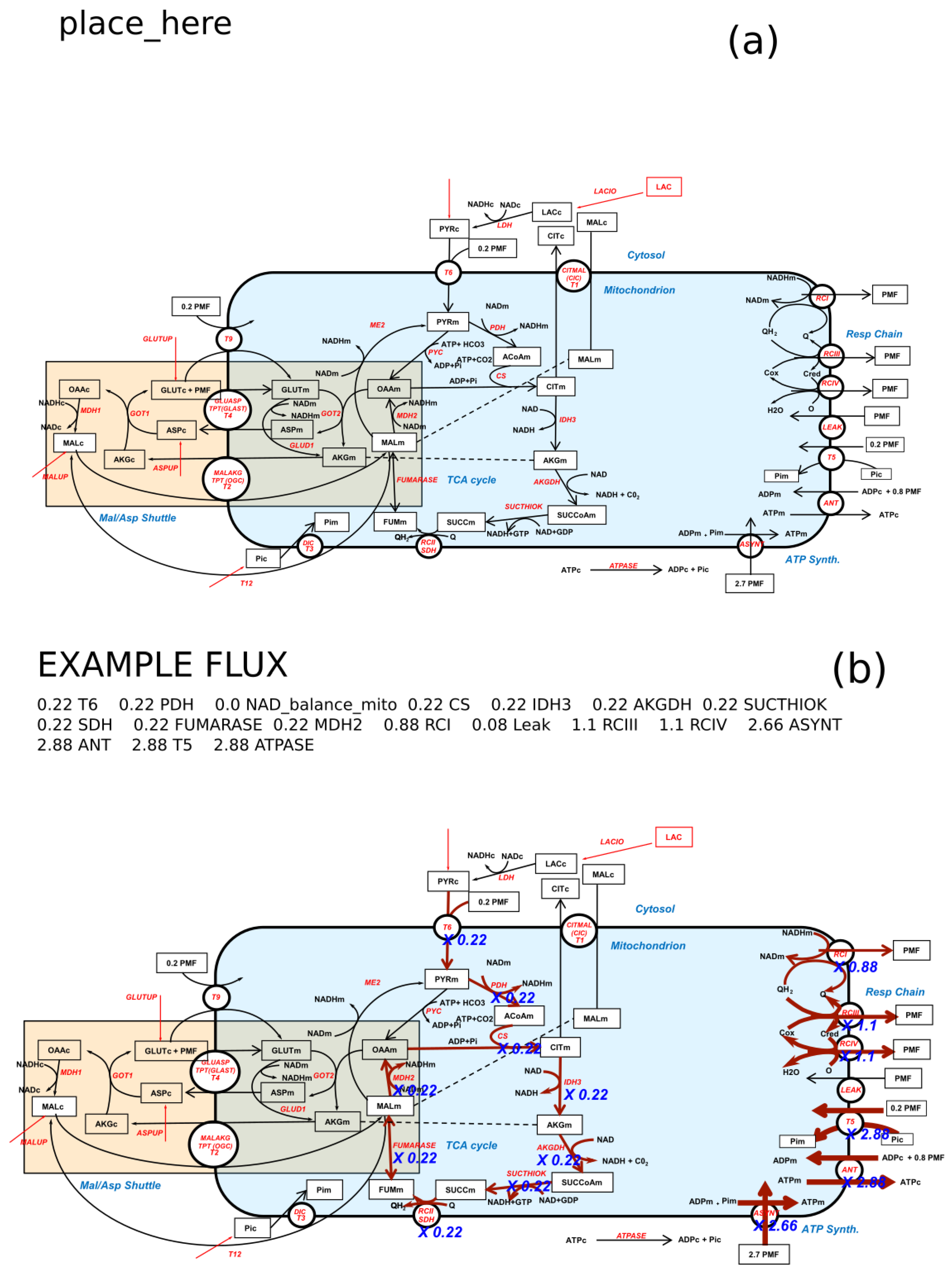
Figure 1 illustrates the idea of the algorithm. Starting from a SVG image of the metabolic network (Figure 1a) an “Example Flux” is plotted on Figure 1b with the option “Auto width” that automatically adjusts the width of the arrows to the flux values between two chosen extrema. The pathway with the flux values is written in place of the “place-here” label in Figure 1a.
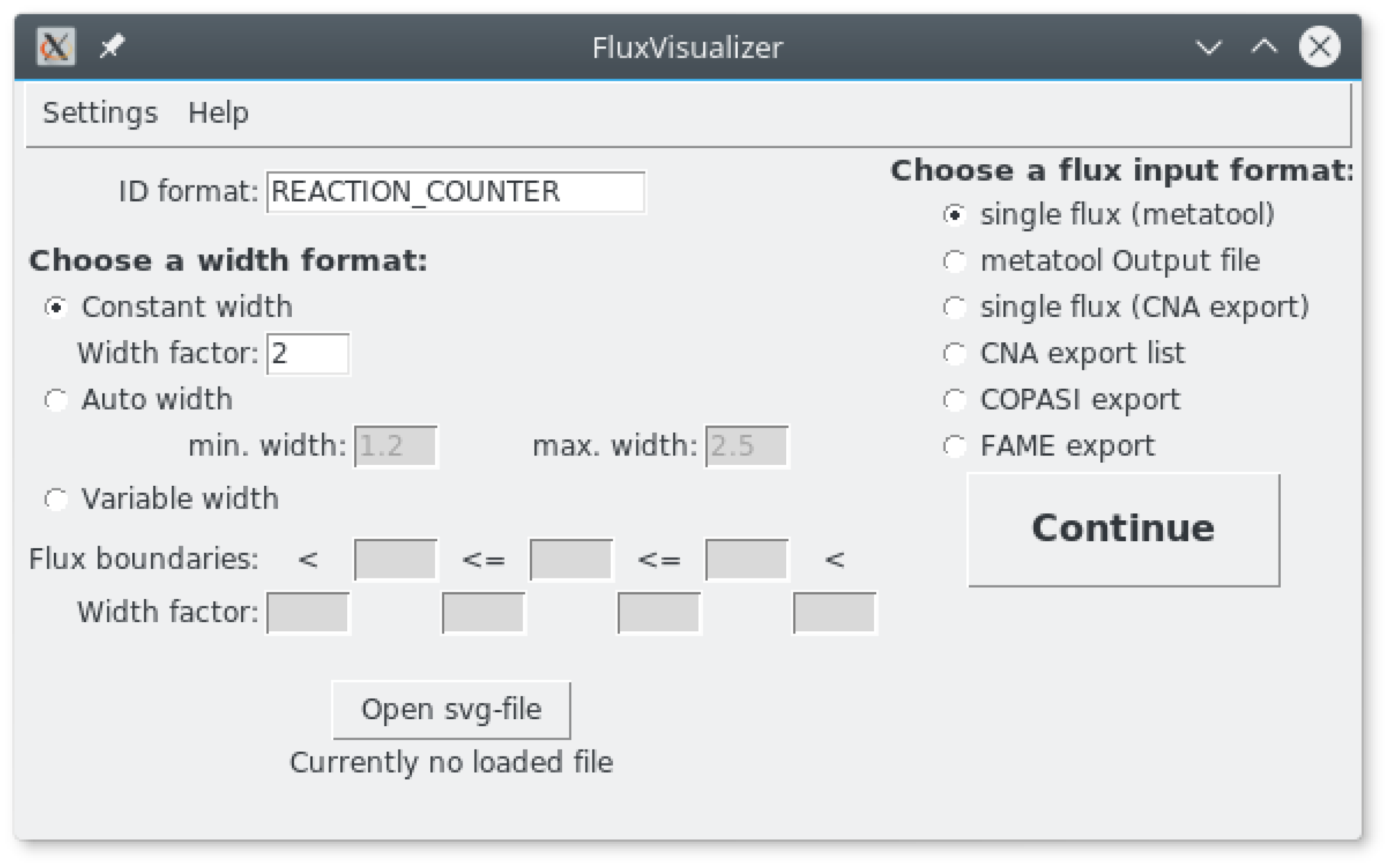
2.1. Main Window (Figure 2)
After starting FluxVisualizer the main window appears (Figure 2). The user can change the ID format and adapt it to the format used in their SVG file. The algorithm will replace the word “REACTION” with the actual reaction name and the word “COUNTER” with a number. To indicate Reversibility the word “REV” has to be added to the ID format (see the manual). All other letters and characters will remain the same for every actual ID in the SVG file. Below the ID format the user has the choice between three ways to define the width factor with which the original width of the arrows is multiplied when a reaction is part of the flux distribution. It is important to mention that all flux constraints and width factors are always considered as absolute flux values (A flux of −5 will have the same width as a flux of 5). This can either be a constant width factor, an automatically fitted width or a variable width. If a constant width is chosen, the arrow widths of the non-zero fluxes are multiplied with the value in the text field “Width factor.” If the “Auto width” is selected, the reaction arrow with the minimum flux (absolute) will be multiplied with the “min. width” value and the maximum value (absolute) will be multiplied with the “max. width” value. The width of all fluxes in between will be obtained by a linear intrapolation in between the minimum and maximum. This option is used to draw the fluxes in Figure 1b showing a broader arrow in reactions RCI (Respiratory Complex I), RCIII (Respiratory Complex III) and so forth (see the right part of the figure) illustrating the high NADH (Reduced Nicotinamide adenine dinucleotide) production by the Krebs cycle giving a higher Oxidative Phosphorylation flux than the Krebs cycle flux. One can also notice a slightly higher flux in RCIII than in RCI due to the entry of succinate in the respiratory chain and the maximum flux for T5, ANT (Adenine Nucleotide Translocator) and ATPSYNT (ATP synthase) evidencing the nearly 3 ATP (Adenosine Triphosphate) synthesized per NADH molecule. This option immediately gives a visual idea of the various fluxes in the network. If the check box “Variable width” is selected, three flux boundaries can be inserted separating four width factors chosen by the user. The program will then visualize the flux with these different widths according to the boundaries in the text boxes. Before proceeding it is necessary to open a SVG image of the network under study. If the image is not readable by the program, opening the file will set up a warning.
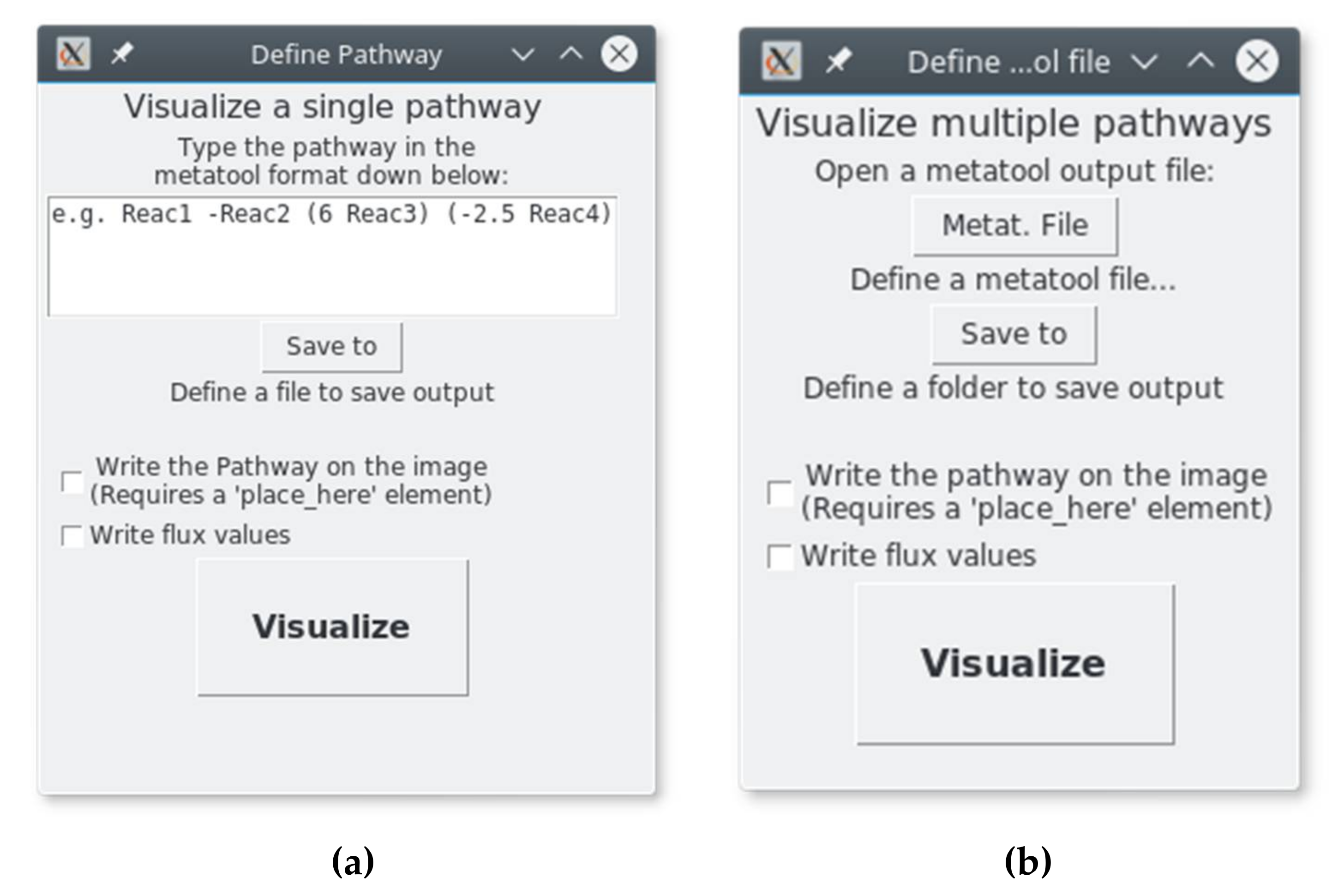
2.2. Secondary Windows (Figure 3)
On the right side of the main window it is possible to decide which input format of the flux distribution will be used. The user can choose between single pathway representations (Figure 3a with different formats: single flux (metatool), single flux (CNA export), COPASI export and FAME export. Conversely metatool and CNA can produce a file containing a series of pathways (EFMs) which can be automatically represented on the same SVG image previously selected in the main window (Figure 2). In this later case, after indicating the input file and the output folder, the series of corresponding SVG images is saved in the output folder (Figure 3b).
2.3. Additional Options
Additional options are proposed on the secondary windows (Figure 3). The first one allows writing the complete pathway with the flux values provided that the “place_here” label exists on the SVG image (see Figure 1). The second option allows writing the flux value on the SVG file below the name of the reaction (see Figure 1). The colour of the arrows of the non-zero fluxes, the size and the number of decimals of the flux values can be defined in the “settings” menu in the main window (Figure 2).
3. Implementation and Requirements
FluxVisualizer is written in Python 3.5.2 (https://www.python.org/) and requires the following modules: tkinter (8.6) lxml (3.5.0) and re (2.2.1). The program, with a manual is freely available at https://fluxvisualizer.ibgc.cnrs.fr.
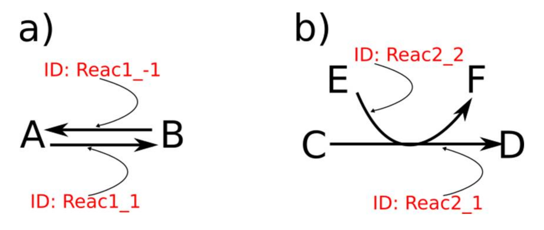
SVG file Requirements: Reactions of the metabolic network are drawn with arrows. Flux through a reaction is visualized by increasing the width of an arrow and/or colouring it. To visualize fluxes, FluxVisualizer needs to recognize the image elements to be changed, essentially the reaction arrow. To this aim, these elements have an annotation ID with the exact name of the reaction as it appears in the pathway entered in the second windows (Figure 3). If it is not the case, (SVG output of another program), ID can be changed easily by any SVG editing tools (Note that MetDraw output [15] can be straightforward used by FluxVisualizer). An example of IDs for reactions is given in Figure 4. The default ID format is REACTION_COUNTER where REACTION will be replaced by the actual reaction name and COUNTER will be replaced by a number (In case that a reaction consists of several arrows (Figure 4b)). Another important parameter is the word REV. It indicates reversibility of reactions. It is part of the ID and if a reaction has a positive flux, it will be removed; if a reaction has a negative flux, it will be replaced by a “-”. An example of reversibility (ID format: REACTION_REVCOUNTER) is given in Figure 4 on the left side and its use on Figure 5. A COUNTER is not required but if a counter is used, it must be used for every reaction ID, even if the reaction consists only of one arrow.
Reaction Names (optional): The reaction names on the SVG representation are necessary if you want to write down the flux values on the SVG image. The ID must be identical to the reaction name (without the counter and additional characters). It must be in a SVG tspan element of a text element. The SVG tspan element of the reaction name is not allowed to carry any other text than the reaction name.
Placing the Flux text (optional): It is also possible to write down the flux distribution as text on the image. To enable this the network file requires a text element saying: “place_here” (Figure 1a). This text element fulfils the same constraints as the reaction names mentioned above. At the position of this text element, the program will write down the flux distribution (Figure 1b, the text “place_here” in (a) is replaced by “Example Flux: 0.22 T6 ...” in (b)).
4. Discussion and Conclusions
As mentioned in the introduction, many software already exists to automatically generate flux maps in metabolic network (at the genome-scale level or not). Usually they are able to draw the entire metabolic network and the pathways of interest with possibly several layouts and zoom functions.
However, there is, among biochemists, a long tradition of metabolic network representation with simple arrows as exemplified in biochemistry textbooks (and in Figure 1 and Figure 5) with particular disposition in space. A simple vertical line with a circle underneath irreversibly evokes glycolysis and the Krebs cycle for a biochemist. It is important to keep this implicit knowledge to facilitate the interpretation of metabolic results or hypotheses. It is undoubtedly the reason why experimental biochemists often draw their own metabolic network representation by hand and report flows also by hand with values and/or colours. This process is tiresome and time-consuming and was automatized with FluxVisualizer. This is why FluxVisualizer does not draw a representation of metabolic networks but starts from the drawings of the biochemist himself with a minimum of constraints.
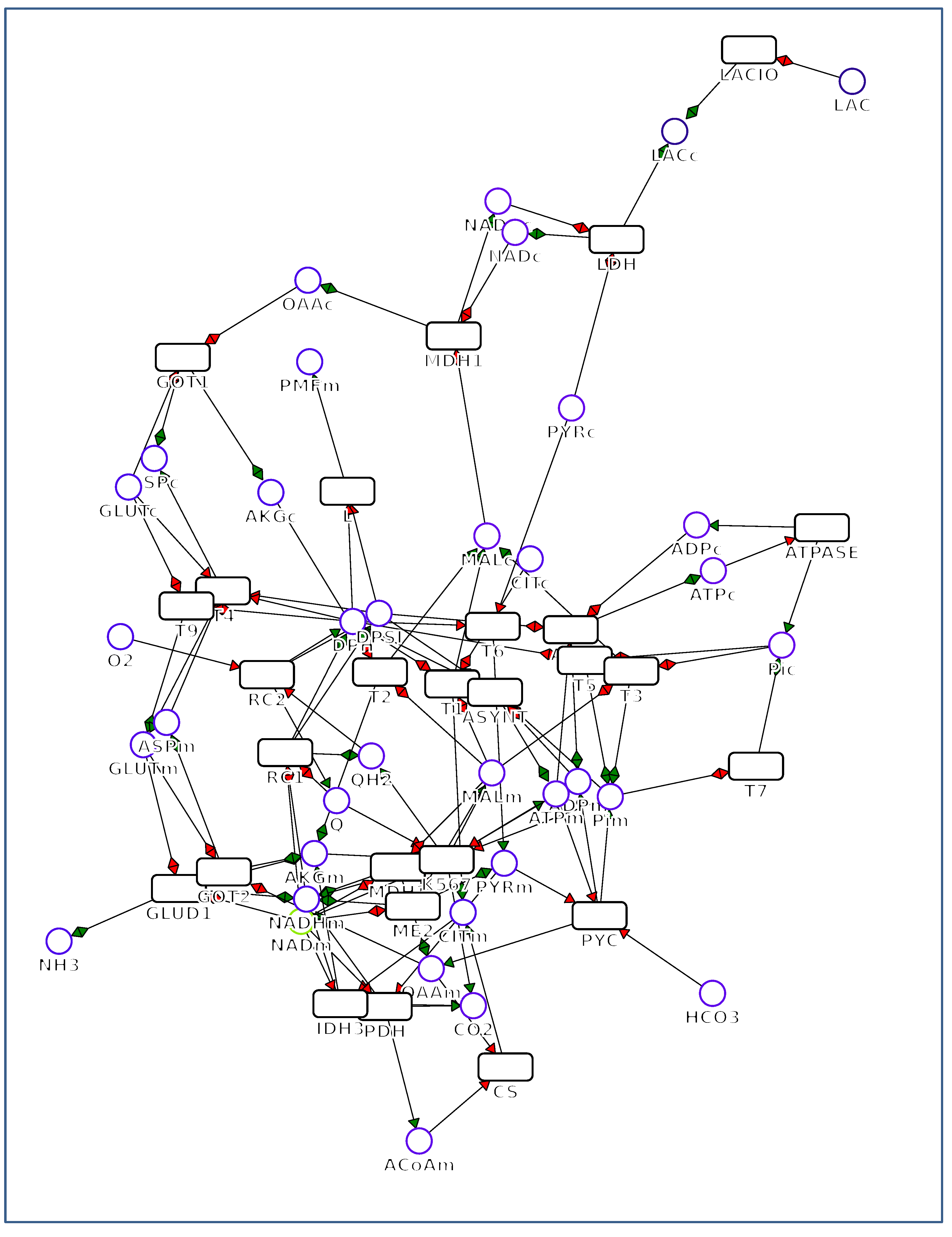
It is thus difficult to compare FluxVisualizer with other software mainly dealing (among other functionalities) with network representation. These software can be used in synergy with FluxVisualizer in providing an SVG representation FluxVisualizer will exploit. This is done on Figure 6 using MetExplore, which is rather easy to use and can export an SVG image, in this case the same metabolic network as in Figure 1a. It must be noted however, that the presence of the nodes, rectangles and circles representing the reactions and metabolites unnecessarily clutters the larger schemes and makes them less readable. Furthermore, it is necessary to re-arrange spatially this diagram to reproduce the biochemist’s layout of Figure 1a. It necessitates a long and tedious work. Undeniably, SVG representation is not (yet) a standard among experimental biologists and this requirement may turn off biologists from FluxVisualizer use, contradicting the purpose of FluxVisualizer to be tailored to biochemists. This is a difficulty for a biochemist to a friendly use of FluxVisualizer. There is another way to take this deterrent step forward. Very often, biologists use LibreOffice (https://fr.libreoffice.org) (or Microsoft Office (https://products.office.com)) suite to draw their diagrams of metabolic networks. It is easy to save them in the pdf format which can be read by Inkscape, for instance, and be converted to the SVG format. This was done in the case of Figure 1 which, initially, was a PowerPoint file. It is then necessary to check the arrow’s ID in order for them to match exactly the name of the reaction. The last solution is to build directly the diagram with Inkscape, for instance, which is not so difficult to manage. This was done for Figure 5.
Another difficulty in visualizing the FluxVisualizer results are the overlaps of the flux values with the rest of the initial image (see Figure 1b). These unescapable overlaps, are not too troublesome for small metabolic networks for which the attribution of a flux value to an enzymatic step remains clear but it is a limit in the size of the network. These overlaps cannot be avoided in an automatic process but their effects can be diminished in playing with the different options of positioning the flux values offered in FluxVisualizer.
Although there is, in principle, no limit in the size of the metabolic network that FluxVisualizer can deal with (genome-scale network should be, in principle, handled) the increasing number of overlaps will decrease the readability of the results on the metabolic network as the number of steps increases. It is difficult to define a precise limit in size and data. Typically, the field of use of this software consists of metabolic networks between a few steps (around 10) to less than 200 reactions, which is probably the limit for a discriminating visualization. This is also the range of the size of customer’s network in the literature (mainly between 10 and 50 which can already generate a very great number of EFMs and possible solutions).
To sum it up, we think that FluxVisualizer fulfils the two aims stated in the introduction: (i) use the biochemist’s own diagram and to replace a tedious manual operation of colouring or/and resizing steps by hand with a fast automatic process and (ii) automatically deliver a series of pathway representations of the same metabolic map from a text list of these pathways (EFMs for instance). This is a great time saver that justifies the time spent presenting the metabolic network in SVG format. We believe that this simple software, freely available at https://fluxvisualizer.ibgc.cnrs.fr, has its place in the theoretical toolbox of the experimental biochemist.
Acknowledgments
Supported by the Plan cancer 2014–2019 No BIO 2014 06 and the French Association against Myopathies. We thank Axel Cattouillart for his technical assistance, Sylvain Prigent for his help in manipulating other tools, Anne Devin for her criticisms and English review and Oliver Ebenhoeh as TDR’s teacher.
Author Contributions
Tim Daniel Rose developed FluxVisualizer, wrote the manual and participated to the redaction of the paper. Jean-Pierre Mazat conceived the project and wrote the paper.
Conflicts of Interest
The authors declare no conflict of interest.
References
- Gehlenborg, N.; O’Donoghue, S.; Baliga, N.S.; Goesmann, A.; Hibbs, M.A.; Kitano, H.; Kohlbacher, O.; Neuweger, H.; Schneider, R.; Tenenbaum, D.; et al. Visualization of omics data for systems biology. Nat. Methods 2010, 7, S56–S68. [Google Scholar] [CrossRef] [PubMed]
- O’Donoghue, S.I.; Baldi, B.F.; Maier-Hein, L.; Stenau, E.; Hogan, J.M.; Humphrey, S.; Kaur, S.; McCarthy, D.J.; Moore, W.J.; Procter, J.B.; et al. Visualization of Biomedical Data. Annu. Rev. Biomed. Data Sci. 2018, in press. [Google Scholar]
- Schellenberger, J.; Park, J.O.; Conrad, T.M.; Palsson, B.Ø. BiGG: A Biochemical Genetic and Genomic knowledgebase of large scale metabolic reconstructions. BMC Bioinform. 2010, 11, 213. [Google Scholar] [CrossRef] [PubMed]
- Maarleveld, T.R.; Khandelwal, R.A.; Olivier, B.G.; Teusink, B.; Bruggeman, F.J. Basic concepts and principles of stoichiometric modeling of metabolic networks. Biotechnol. J. 2013, 8, 997–1008. [Google Scholar] [CrossRef] [PubMed]
- Antoniewicz, M.R. Methods and advances in metabolic flux analysis: A mini-review. J. Ind. Microb. Biotechnol. 2015, 42, 317–325. [Google Scholar] [CrossRef] [PubMed]
- Kacser, H.; Burns, J.A. The control of flux. Symp. Soc. Exp. Biol. 1973, 32, 65–104. [Google Scholar] [CrossRef]
- Heinrich, R.; Rapoport, T.A. A linear steady-state treatment of enzymatic chains; its application for the analysis of the crossover theorem and of the glycolysis of human erythrocytes. Acta Biol. Med. Ger. 1973, 31, 479–494. [Google Scholar] [PubMed]
- Reder, C. Metabolic control theory: A structural approach. J. Theor. Biol. 1988, 135, 175–201. [Google Scholar] [CrossRef]
- Sauro, H. Systems Biology: Introduction to Pathway Modeling; Ambrosius Publishing: Bangalore, India, 2014; ISBN 978-0-9824773-7-3. [Google Scholar]
- Klipp, E.; Liebermeister, W.; Wierling, C.; Kowald, A. Systems Biology: A Textbook, 2nd ed.; Wiley-Blackwell: Berlin, Germany, 2016; ISBN 978-3-527-33636-4. [Google Scholar]
- Ataman, M.; Hernandez Gardiol, D.F.; Fengos, G.; Hatzimanikatis, V. redGEM: Systematic reduction and analysis of genome-scale metabolic reconstructions for development of consistent core metabolic models. PLoS Comput. Biol. 2017, 13, e1005444. [Google Scholar] [CrossRef] [PubMed]
- Smith, A.C.; Eyassu, F.; Mazat, J.-P.; Robinson, A.J. MitoCore: A curated constraint-based model for simulating human central metabolism. BMC Syst. Biol. 2017, 11, 114. [Google Scholar] [CrossRef] [PubMed]
- Orth, J.; Fleming, R.; Palsson, B. Reconstruction and Use of Microbial Metabolic Networks: The Core Escherichia coli Metabolic Model as an Educational Guide. EcoSal Plus 2010. [Google Scholar] [CrossRef] [PubMed]
- Omix Visualization | Welcome. Available online: https://www.omix-visualization.com/ (accessed on 21 April 2018).
- Jensen, P.A.; Papin, J.A. MetDraw: Automated visualization of genome-scale metabolic network reconstructions and high-throughput data. Bioinformatics 2014, 30, 1327–1328. [Google Scholar] [CrossRef] [PubMed]
- Chazalviel, M.; Frainay, C.; Poupin, N.; Vinson, F.; Merlet, B.; Gloaguen, Y.; Cottret, L.; Jourdan, F. MetExploreViz: Web component for interactive metabolic network visualization. Bioinformatics 2017, 34, 312–313. [Google Scholar] [CrossRef] [PubMed]
- König, M.; Holzhütter, H.G. Fluxviz—Cytoscape plug-in for visualization of flux distributions in networks. Genome Inform. 2010, 24, 96–103. [Google Scholar] [PubMed]
- Granger, B.R.; Chang, Y.C.; Wang, Y.; DeLisi, C.; Segrè, D.; Hu, Z. Visualization of metabolic interaction networks in microbial communities using VisANT 5.0. PLoS Comput. Boil. 2016, 12, e1004875. [Google Scholar] [CrossRef] [PubMed]
- Turkay, C.; Jeanquartier, F.; Holzinger, A.; Hauser, H. On computationally-enhanced visual analysis of heterogeneous data and its application in biomedical informatics. In Interactive Knowledge Discovery and Data Mining in Biomedical Informatics; Holzinger, A., Jurisica, I., Eds.; Springer: Berlin/Heidelberg, Germany, 2014; pp. 117–140. [Google Scholar]
- Pfeiffer, T.; Sánchez-Valdenebro, I.; Nuño, J.C.; Montero, F.; Schuster, S. METATOOL: For studying metabolic networks. Bioinformatics 1999, 15, 251–257. [Google Scholar] [CrossRef] [PubMed]
- Klamt, S.; Saez-Rodriguez, J.; Gilles, E.D. Structural and functional analysis of cellular networks with CellNetAnalyzer. BMC Syst. Biol. 2007, 1, 2. [Google Scholar] [CrossRef] [PubMed]
- Hoops, S.; Sahle, S.; Gauges, R.; Lee, C.; Pahle, J.; Simus, N.; Singhal, M.; Xu, L.; Mendes, P.; Kummer, U. COPASI—A COmplex PAthway SImulator. Bioinformatics 2006, 22, 3067–3074. [Google Scholar] [CrossRef] [PubMed]
- Boele, J.; Olivier, B.G.; Teusink, B. FAME, the Flux Analysis and Modeling Environment. BMC Syst. Biol. 2012, 6, 8. [Google Scholar] [CrossRef] [PubMed]
Figure 1.
An example of customer’s metabolic network as an SVG file (a) and (b) after the visualization of the pathway 0.22 T6…. on this SVG image with the “Auto width” option. The width of the fluxes is proportional to the coefficient of the step between the min. width 1.5 and the max. width: 3.0. Note that the flux values are written in blue italic along the reactions arrows and that the complete pathway is written in the place of the “place_here” label in (a). The light blue background represents mitochondrion and the light brown background depicts the Malate Aspartate Shuttle (MAS) connecting the redox status of cytosol and mitochondria.

Figure 2.
Main window of FluxVisualizer showing the various width formats on the left and the different input formats on the right.
Figure 2.
Main window of FluxVisualizer showing the various width formats on the left and the different input formats on the right.

Figure 3.
Windows appearing after the user has pressed the “continue” button in the main window. By closing the windows in the upper right corner, the user goes back to the main window (Figure 2). The (a) figure concerns the single pathway representation on a single SVG image. The (b) figure concerns the case of a list of pathways (metatool or CNA format) corresponding to a series of SVG images automatically created and saved in a folder.

Figure 4.
(a) A simple example of IDs of reaction arrows with reversibility (ID format: REACTION_REVCOUNTER) and (b) with several arrows for one reaction (ID format: REACTION_COUNTER).
Figure 4.
(a) A simple example of IDs of reaction arrows with reversibility (ID format: REACTION_REVCOUNTER) and (b) with several arrows for one reaction (ID format: REACTION_COUNTER).

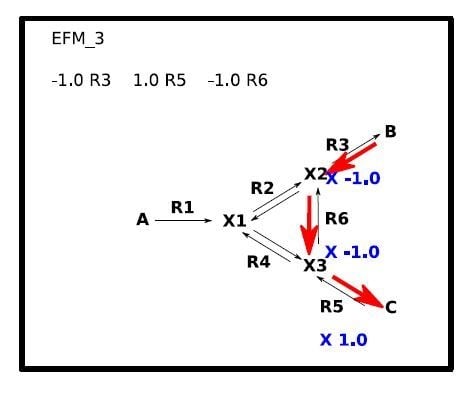
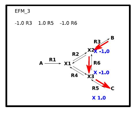
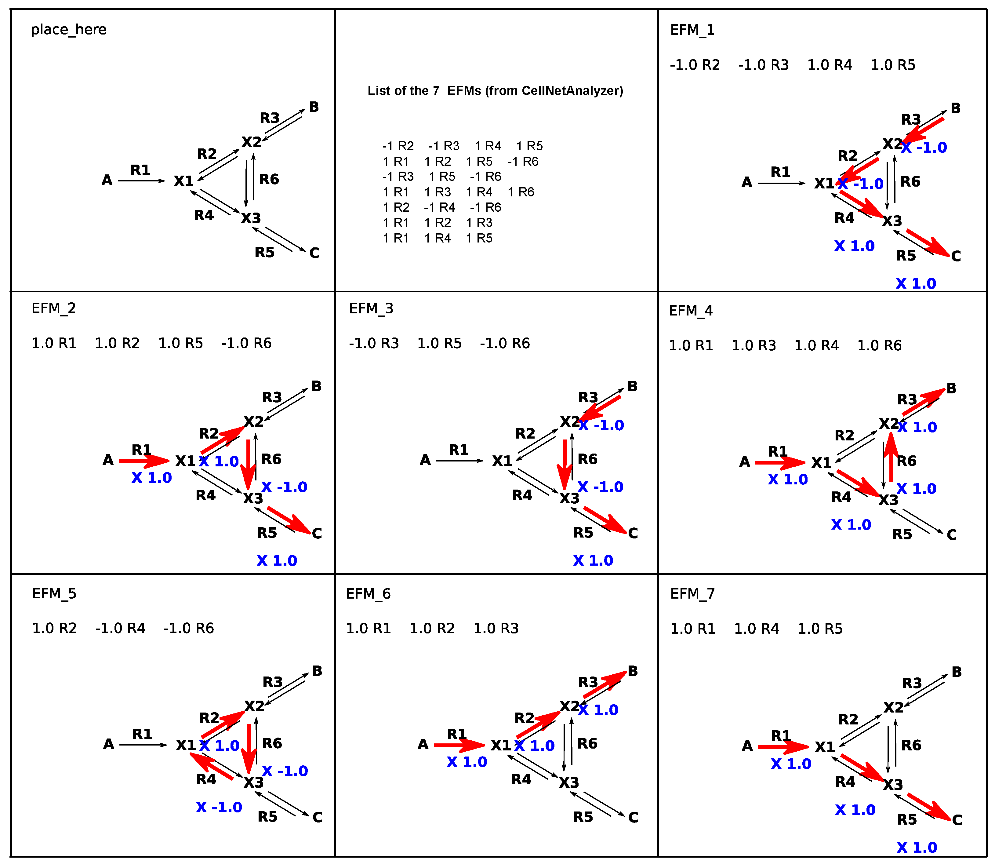
Figure 5.
A simple example of the generation of Elementary Mode of Flux (EFMs) representation. The customer’s SVG (Scalable Vector Graphics) file is given in the top left of the figure (labelled ‘place_here’). The list of EFMs from CellNetAnalyzer in this form is in middle top images. With the option ‘cna (CellNetAnalyzer) export list’ (Figure 2) this list is entered as CNA file (Figure 3a) and generates the successive EFMs, EFM_1 until EFM_7.

Figure 6.
SVG representation of the network of Figure 1a with MetExplore, which is representative of most of the software cited in the text. The red arrows correspond to substrates and the green ones to products of the reactions in rectangles. The metabolites are indicated with circles.
Figure 6.
SVG representation of the network of Figure 1a with MetExplore, which is representative of most of the software cited in the text. The red arrows correspond to substrates and the green ones to products of the reactions in rectangles. The metabolites are indicated with circles.

© 2018 by the authors. Licensee MDPI, Basel, Switzerland. This article is an open access article distributed under the terms and conditions of the Creative Commons Attribution (CC BY) license (http://creativecommons.org/licenses/by/4.0/).
Share and Cite
MDPI and ACS Style
Rose, T.D.; Mazat, J.-P. FluxVisualizer, a Software to Visualize Fluxes through Metabolic Networks. Processes 2018, 6, 39. https://doi.org/10.3390/pr6050039
AMA Style
Rose TD, Mazat J-P. FluxVisualizer, a Software to Visualize Fluxes through Metabolic Networks. Processes. 2018; 6(5):39. https://doi.org/10.3390/pr6050039
Chicago/Turabian StyleRose, Tim Daniel, and Jean-Pierre Mazat. 2018. "FluxVisualizer, a Software to Visualize Fluxes through Metabolic Networks" Processes 6, no. 5: 39. https://doi.org/10.3390/pr6050039
Note that from the first issue of 2016, this journal uses article numbers instead of page numbers. See further details here.