A Differentiable Model for Optimizing Hybridization of Industrial Process Heat Systems with Concentrating Solar Thermal Power


Process Systems and Operations Research Laboratory, UTC Institute for Advanced Systems Engineering and Department of Chemical and Biomolecular Engineering, University of Connecticut, Storrs, CT 06269, USA
Processes 2018, 6(7), 76; https://doi.org/10.3390/pr6070076
Submission received: 6 June 2018
/
Revised: 18 June 2018
/
Accepted: 19 June 2018
/
Published: 23 June 2018
(This article belongs to the Special Issue Modeling and Simulation of Energy Systems)
Abstract
:A dynamic model of a concentrating solar thermal array and thermal energy storage system is presented that is differentiable in the design decision variables: solar aperture area and thermal energy storage capacity. The model takes as input the geographic location of the system of interest and the corresponding discrete hourly solar insolation data, and calculates the annual thermal and economic performance of a particular design. The model is formulated for use in determining optimal hybridization strategies for industrial process heat applications using deterministic gradient-based optimization algorithms. Both convex and nonconvex problem formulations are presented. To demonstrate the practicability of the models, they were applied to four different case studies for three disparate geographic locations in the US. The corresponding optimal design problems were solved to global optimality using deterministic gradient-based optimization algorithms. The model and optimization-based analysis provide a rigorous quantitative design and investment decision-making framework for engineering design and project investment workflows.
1. Introduction
Industrial process systems are enormous consumers of energy (9.23 TWh), accounting for roughly one-third of all delivered energy use (28.64 TWh) in the United States in 2017 [1]. Roughly 60% of the energy consumption in the industrial sector is from the manufacturing sector, which accounts for roughly 20% of the total US energy consumption [2]. The industrial sector has historically been the largest consumer of natural gas [1] as both a feedstock and a primary energy source. In manufacturing, industrial process heat (IPH) accounts for roughly 70% of the total process energy consumed in the US [3]. When broken down by fuel consumption, the manufacturing sector accounts for roughly 95% of all IPH demand in the US [3]. Further, since the majority of these process systems require low- or medium-temperature process heat (<250 C) [3,4], there is a substantial opportunity to reduce fossil fuel consumption and carbon emissions by augmenting existing IPH systems with solar thermal power and designing new systems incorporating solar thermal power.
Numerous studies have been conducted over the past 40 years on the potential that solar energy can play within IPH systems [4,5,6,7,8,9]. Active interest in the topic in recent years has been motivated largely by the concern over unsustainable energy consumption, greenhouse gas emissions, and overall environmental impact of commercial and industrial sectors [10]. Attention to the feasibility of solar applications to specific industries has been made, such as: food and beverage [11], mining [12,13], agriculture [14,15], textiles [11,16,17,18,19], pulp and paper [20,21], chemicals [22,23], and building construction materials [4], among others. Recent reviews [4,6,7,9] resolve the individual industries by their similar unit operations (e.g., drying, hot water, sterilization, etc.). Results of such studies indicate general feasibility of solar in IPH applications; however, the economic viability is extremely sensitive to the application and geographic region of the project. Given the diversity of IPH demand profiles across industries and applications as well as the widely-varying solar resource performance profiles across geographic locations, a formal numerical simulation and optimization-based design approach is necessary to ensure the economic viability of hybrid solar-IPH systems.
Modeling, Simulation, and Optimization
Numerous models with varying levels of complexity and usage scenarios have been proposed for the design and simulation of solar thermal energy systems [24,25,26,27,28,29,30,31,32,33,34,35,36,37]. Specifically, the focus of this paper is on the application of modeling and simulation for mathematical optimization-based design of solar-IPH systems.
A formal mathematical optimization approach was applied by Ghobeity and Mitsos [28] to the design and operation of a solar thermal receiver and thermal energy storage (TES) system with a constant IPH demand for high-temperature steam generation (for power cycles). A sequential design approach was applied that first considers minimizing total solar cost with the solar array size and TES capacity as design decision variables and several operating decision variables related to the proposed dynamical model [28]. The model was developed for use with gradient-based local optimization solvers and utilized a total daily concentrated energy value based on a single winter day and a heliostat field efficiency calculated for a location in Cyprus [28]. The economic objective was considered as a simple linear cost model with fixed specific costs for the TES medium and solar array. The second optimization problem considered the yearly operation for the fixed design based on the winter day. Thus, for the fixed design, feasible optimal operating conditions were found with respect to 12 representative days throughout the year [28].
Modeling and simulation for hybridizing power cycles with concentrating solar thermal (CST) power was recently considered by Gunasekaran and coworkers [30] with system optimization by Ghasemi and coworkers [29] and Ayub and coworkers [36]. In [29], the focus was on optimizing the operation of the hybrid system without considering TES. In [36], economics were considered to optimize the levelized cost of electricity. However, due to the regional dependence of the solar model and economic assumptions, optimization with respect to the economics of the parabolic trough solar concentrator (PTC) array sizing were omitted. Additionally, in [36], no TES was considered. The thermo-economic model was implemented in Engineering Equation Solver (EES) and a shortcut method is used to optimize the hybrid system using intermediate variables calculated from the AspenPlus sequential-quadratic programming (SQP) optimizer.
A simplified approach to the optimal design of solar water heating systems was presented by Yan et al. [33]. The authors developed a high-level energy conservation model of the water heating system including TES as a hot water tank. The design decision variables were taken as the array size and the TES capacity and the objective was the lifecycle savings. The authors [33] proposed an approach based on diminishing marginal utility and identified optimal solutions based on the intersection of marginal energy savings and marginal embodied energy curves. Although their simplified approach was effective for the water-heating application, IPH applications and their dramatically differing energy demand profiles complicate the optimal design problem as the total utilizable energy and lifecycle savings exhibit large degrees of nonlinear sensitivity to the decision variables [33].
A hybrid solar-IPH design strategy based on heat integration was considered by Baniassadi et al. [34]. The authors considered fixed array designs determined by maximizing the solar fraction for a particular pre-determined investment and analyzed the various options for coupling solar energy with process streams. They proposed an algorithm which uses the various process stream temperatures and pinch analysis to identify the best process stream to exchange solar energy with. They utilized a commercial simulator to calculate the performance of the solar system and subsequently the economics of the retrofit strategy [34]. Although the analysis identifies some technical challenges of physically coupling the solar thermal system with the process from a heat integration perspective, it does not adequately address the fundamental design considerations of the solar system itself [34]. Further, their approach cannot be used within mathematical optimization-based design strategies as the solar performance model is only accessible as an ad-hoc black-box simulation [34].
In [31], Silva and coworkers considered a formal simulation and optimization-based design approach to hybrid solar-IPH systems. In their work, a single-tank thermocline TES device was modeled along with a PTC array for medium-temperature (100–250 C) IPH applications. Three economic objective functions were considered: levelized cost of energy, payback time, and lifecycle savings as their base case [31]. Four design variables were considered in their work: the number of PTC modules in series, the number of PTC modules in parallel, the spacing between the rows, and the TES capacity [31]. The authors propose a derivative-free non-deterministic memetic optimization algorithm based on a modified genetic algorithm [31]. They make explicitly clear that this approach is in response to the major challenges in optimizing dynamical systems based on simulation: possible discontinuities, nonlinearity, and expensive complex objective function evaluations [31].
In [32], a hybrid solar-IPH system for zero-liquid discharge desalination (<250 C) was considered. Similar to [31], a formal simulation and optimization-based design approach was taken using the net-present value as the economic objective. The design variables considered for the base-case were the number of PTC modules and the TES capacity. A formal robust design problem was considered as a nonconvex non-cooperative game by taking into account uncertainty in the natural gas and product markets and solving the problem formulated as a semi-infinite program [32]. Again, the authors note that due to the non-differentiable nature of the model, a derivative-free genetic algorithm-based optimization approach must be used with subsequent analysis to verify feasibility and optimality of solutions [32].
The past approaches to modeling, simulation, and optimization of solar-IPH systems have all shown favorable results using model formulations or approaches specific to the application of interest or more general formulations which pose challenges for deterministic gradient-based optimization. There exists a need for a dynamic model of a CST-TES system for designing optimal hybrid solar-IPH systems with accurate economic models for assessing technology investment risk and the economic viability of such projects. In this paper, a model is developed for low- to medium-temperature CST-TES systems for assessing the economic viability and overall project feasibility of hybrid solar-IPH systems. The model accounts for a single-axis tracking PTC array, a TES device, and utilizes high-accuracy hourly solar resource data for the United States available from an open-access database. The model is developed specifically for use with deterministic (global) optimization algorithms, and therefore accounts for convex analysis, differentiability, and the trade-offs between computational efficiency and model accuracy.
In Section 2, the hybrid solar-IPH process performance model will be developed which includes a smooth formulation, a model of a PTC with solar angle calculations for high-resolution dynamic simulation of CST performance, an economic model for assessing design feasibility and investment decision-making, and a mathematical optimization formulation. Additionally, the key theoretical results and analysis of the model are presented in Section 2. In Section 3, four numerical case studies for varying fuel costs and IPH demand profiles across three geographically-disparate locations are presented and discussed followed by the Conclusion in Section 4.
2. Model Formulations
2.1. Concentrating Solar Thermal Model
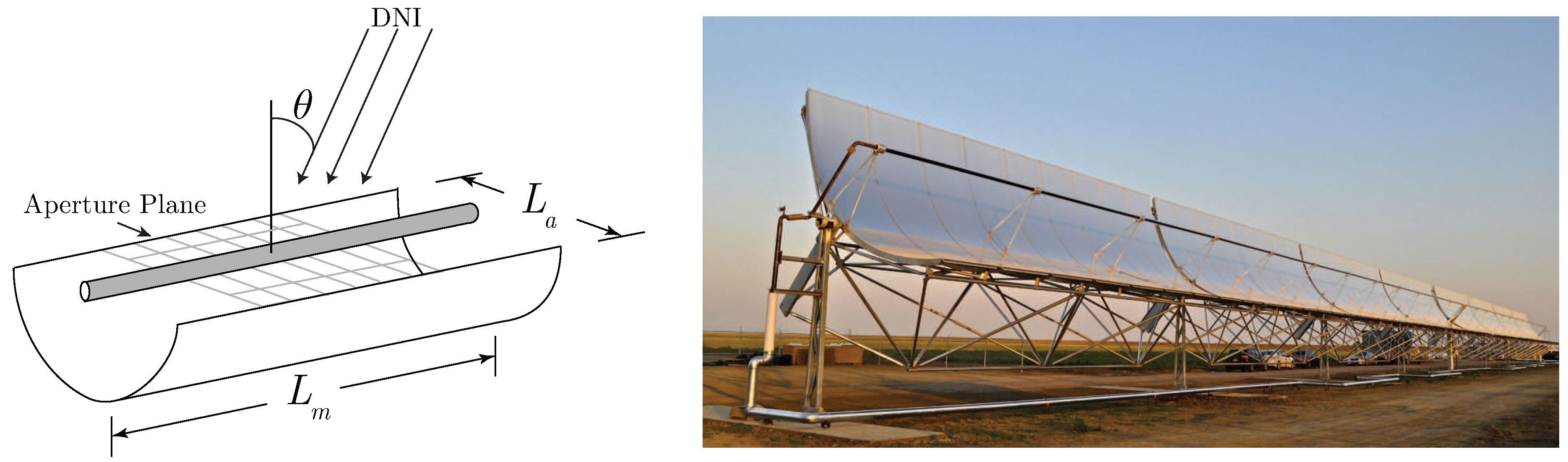
For a surface or defined geometry oriented horizontally, the performance of the solar energy collector relies on the surface tilt angle and the incidence angle of the irradiation striking the surface. Here, we consider the model of a PTC, illustrated in Figure 1 with the aperture area of a single trough given by . The total optical efficiency of the reflector is defined in the following.
Definition 1
(Optical Efficiency, ηopt [30]). The optical efficiency of the PTC is given by:
where for are efficiency factors related to various components of the PTC and the incidence angle modifier K is given by the empirical relationship [39,40]:
Here, is the shadowing factor of the receiver tube (=0 for fully-shadowed and =1 for no shadowing), is the tracking error factor (=1 for no tracking error), is the geometry error (=1 for no geometric or mirror alignment errors), is the mirror dirt factor (=1 for perfectly clean mirrors), is the dirt factor for the glass envelope enclosing the receiver tube (=1 for perfectly clean glass), and are the unaccounted for losses (=1 for no unaccounted losses). The factor is the reflectance of perfectly clean mirrors (=1 for 100% reflectance), is the absorptance of the receiver tube itself (=1 for a perfect black-body), and τ is the transmittance of the glass envelope enclosing the receiver tube. The factor K accounts for the fact that irradiance is not normal to the PTC aperture (unless the array has two-axis tracking). The incidence angle θ follows from the solar position model in Appendix A.
With the above quantities, the specific thermal power potential (in units of kW/m) is given by
with the direct-normal irradiance (DNI) at a particular moment in time and geographic location (in standard units of W/m). Note the DNI values come from experimental measurements. These values are available for specific geographic locations in the US (and some international regions) for annual time horizons with hourly resolution (i.e., 8760 discrete hourly values), via the National Renewable Energy Laboratory’s (NREL) National Solar Radiation Database (NSRDB) [41]. In this work, a geographic location is specified and the typical meteorological year (TMY) data is downloaded. The numerical values of the PTC modeling parameters used in this study can be found in Table A1 of Appendix B. Finally, the solar thermal power produced (in units of kW) by a solar array is given by
with as the total aperture area of the solar array.
2.2. Process System Model
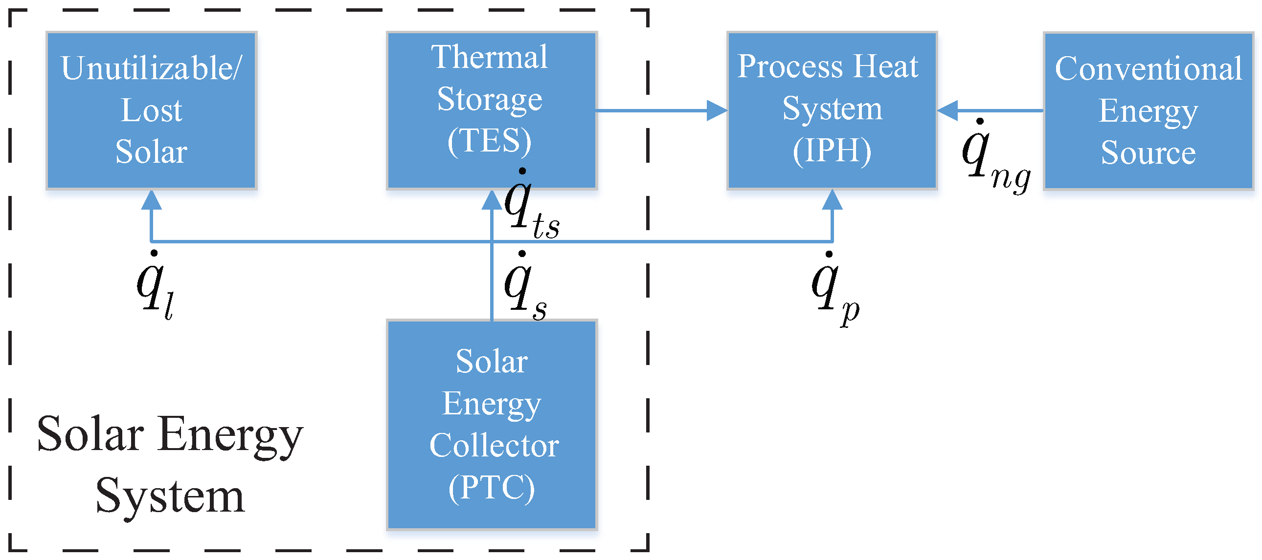
The process system of interest is represented by the block-flow diagram in Figure 2. Physically, the system consists of the solar energy collector as the source of solar thermal energy for the system, the TES, the IPH system which exists as an energy demand, and the conventional (fossil) energy source for times of inadequate solar energy.
The process system model is developed from a high-level with the following simplifying assumptions:
- Heat losses to the environment from piping and heat exchangers is negligible.
- Heat losses to the environment from the TES is negligible.
- The process system requires low to medium temperature IPH (i.e., ≤250 C).
- Heat is always available at or above the minimum temperature as required by the IPH system.
- The IPH system energy demand is not dependent on the state or design decisions of the solar energy system.
Under these assumptions, the process system model is developed from the overall energy balance on the entire system:
where is the instantaneous thermal power provided by the solar system, is the instantaneous thermal power provided by the conventional fossil-fuel (e.g., natural gas) heating system, is the instantaneous thermal power demand by the industrial process (IPH), is the instantaneous power supply/demand of the solar thermal energy storage system, and is the lost solar thermal power due to meeting the IPH requirements and reaching the maximum thermal storage capacity (i.e., the unutilizable solar energy). Note that can be both positive (charging state) and negative (discharging state).
The complicating details for accounting for energy in the system comes from the capacity limitations of the TES. For example, without TES, the solar array will simply deliver all its energy to the IPH system until the full power demand is met. At which point, the solar array will simply de-focus, or we account for the positive difference between the supply and demand as losses or unutilizable solar . The negative difference between the supply and demand is simply accounted for by the conventional heating system . However, with the existence of a TES device, the positive difference between solar thermal power supply and IPH demand can be stored and used in future times when the solar system alone cannot meet the IPH demand. This complicates the model since we assert a preference for solar energy over conventional energy sources, and hence must account for the finite capacity of the storage device and its stored capacity at each instant in time.
Rearranging Equation (4) to focus on the storage device, we get:
where we have introduced for ancillary energy accounting. Physically, this quantity is used for load balancing control (i.e., balancing energy supply and demand). Equivalently, we write:
assuming the TES device is empty at the start of the simulation. Applying the explicit Euler integration scheme with as the discrete time step-size (1 h for standard solar data), we can write:
Next, we develop the model to account for the finite capacity of the TES device. Since we know that the energy capacity of the TES device at any instant can only take values between zero and the maximum capacity, we write:
where is the storage capacity variable scaled in hours of peak process demand , determined by the process operations schedule model (known a priori). The inner max binary operation accounts for the condition that if there was excess energy available from the combined solar array and TES at the previous time, then we should consider storing it for future use. The outer min binary operation accounts for the condition that, if we are considering storing energy, we can only store at or below the maximum TES capacity. Equivalently, we can write
where the mid operator selects the median value of the three arguments. Combining Equations (5)–(7), the overall energy balance becomes:
From this model, there are three possible states from the load-balancing perspective at each discrete time point i:
- The PTC is not providing enough energy to meet the demand of the process (TES moves into the discharging state) and there is not enough energy in the TES to meet the demand of the process over this time step. In this case, conventional energy must be supplied to the process to meet the full demand of the process.
- The PTC is providing enough energy to meet the demand of the process (TES moves into the charging state) and there is not enough available capacity to store all excess energy in the TES device. In this case, the excess energy must be rejected.
- The TES is either in the discharging state with enough stored energy to meet the full demand, or it is in the charging state and has enough available capacity to store the solar energy in excess of the process demand.
With these relationships, we can write:
so that and are accurately accounted for. At any given discrete time point, we have the following relationship for load balancing:
Note that losses are accounted for here as simply the unutilizable solar power at any given time step and do not account for standard thermal losses to the environment which occur in thermal systems. As stated previously, heat losses for the TES are expected to be minimal over the timescale of charging/discharging cycles. This is valid for well-insulated systems that undergo complete or nearly-complete discharge over the course of the day. For systems that have long-term (i.e., many days or months) storage, this assumption will not be valid. Further, TES systems to be installed outdoors and above-ground may need special consideration of ambient environmental/weather conditions as large temperature swings and high winds may invalidate this assumption as significant heat transfer with the environment may occur. In all cases, some heat losses are expected during the course of operation of the physical systems which will result in an under-sized design proportional to the actual heat losses, under these assumptions.
Additionally, heat losses from piping and heat exchangers are expected to be minimal. Similarly, these assumptions are valid for well-insulated systems. To account for any of these losses, the design engineer may apply higher-fidelity models that take into account operating temperatures, heat exchanger designs, and overall heat transfer coefficients for the system(s) of concern. However, doing so at this stage significantly complicates the model from an optimization perspective and negatively impacts computational tractability. Alternatively, high-fidelity modeling may be used to estimate average losses for a particular geographic region and IPH temperature requirements. These losses can then be accounted for as an overall thermal efficiency and used to adjust the IPH demand accordingly, similar to the factor in the optical efficiency model for the CST array in Equation (1). Finally, to assess the performance of a CST system with respect to its ability to augment the use of conventional energy sources for IPH, we define the annual average solar fraction:
In terms of the discrete values calculated from Equation (8) and the identities in Equation (9), the solar fraction can be approximated numerically using:
which represents the fraction of total energy consumed by the process that is supplied by the solar system over the entire time interval of interest (e.g., a TMY).
Lastly, although it was assumed that is not a function of the state or design decisions of the solar energy system, it need not be constant. For the purposes of studying the effects of transient load demand on the solar hybridization strategy, we will consider the model:
which assumes i is in hours () with corresponding to 1:00 a.m. on 1 January, is the mean IPH demand, and is the fractional deviation from the mean IPH demand. For , this models a constant IPH demand. For , this model accounts for a dynamic ramp-up and ramp-down of demand with a maximum demand at local noon and a minimum demand at local midnight.
To use the developed models effectively within a simulation-based optimization framework, we present the following concavity result for .
Theorem 1.
Let be nonempty compact intervals. The solar fraction is a concave function on its domain.
Proof.
From Equations (7)–(9) and the feasible system states, we can write
for the case (or else ). The physical meaning of this case is that the solar system is producing more thermal power than can be used by the process or stored in the TES, and hence lost/rejected. We can see that is an affine function of and
is a convex function of and . Therefore,
is an affine function of and . Since is the pointwise maximum of an affine function and a constant, it is convex. From Equation (10), we have the summation of the terms:
which is an affine function of subtracting a convex function of and , and hence concave. Finally, since in Equation (10) is a summation of concave functions (the denominator is not a function of or ), it is concave. ☐
Smooth Approximation
Since the energy balance equations from the previous section involve min and max operators, differentiability of as defined in Equation (10) cannot be guaranteed. Since gradient-based optimization algorithms typically require all functions to be at least once-continuously differentiable, we must develop a smooth formulation. Consider the following operator:
as a smooth approximation of the binary max operator: . The maximum error between the max operator and is and occurs at . For , the error approaches zero. Hence, for small values, this approximation is not expected to introduce appreciable error into the model. A smooth approximation of , as defined in Equation (10), is given by:
Again, the motivation of the model development is for use within simulation-based (global) optimization. The following result ensures that the smooth approximation is concave and differentiable.
Theorem 2.
Let be nonempty compact intervals. Then, the smooth solar fraction is concave and continuously differentiable.
Proof.
Let for some i, and . It is clear that f is convex on and is affine. Therefore, is convex for every i. Further, both f and are continuously differentiable on their domains. Therefore, is continuously differentiable on . Since is defined as the sum of the terms
with a constant denominator (with respect to and ), it is concave and continuously differentiable on . ☐
2.3. Economic Model
An economic analysis is at the heart of all new-technology investment decision-making. Therefore, successfully designing a solar-IPH hybridization strategy requires a thorough economic analysis to ensure an optimal venture. Often, such an analysis consists of a comparison of conventional energy prices and the levelized cost of electricity (LCOE) for electrical power systems or the levelized cost of heat (LCOH) for thermal systems. For IPH applications, the LCOH analysis is often appropriate. However, the LCOH is defined at a high-level as:
which cannot be guaranteed to be convex under appropriate assumptions. In contrast, we will develop the economic model of total lifecycle savings (LCS) which represents the total cost savings (which we wish to maximize) realized by hybridizing the IPH system with CSP.
The lifecycle savings is defined as the difference between the total lifetime cost of energy for a conventional system and that of the hybridized system, accounting for the time-value of money and energy-price inflation:
where is simply the vector-form of our decision variables, is the total lifetime of the project in years, r is the discount rate, is the cost of conventional fuel at year i, is the annualized cost of capital including debt service at year i for financing model k, and is the annual operating and maintenance (O&M) cost of the CST-TES system at year i. The solar hybridization design objective then is to maximize , and hence, it is ideal if is concave on its domain. The optimization problem formulation will be discussed in the next section.
The cost of conventional fuel at year i is given by:
where is the current specific thermal energy cost and is an inflation rate on the fuel price. The O&M cost is typically estimated under a fixed-pricing model [42] (i.e., cost per kWh of thermal energy produced).
The annualized capital expenditure and debt service of the CST-TES system at year i is given by [32]:
which assumes monthly-compounded interest at an annual rate of , over the loan term (in years). The term is the total capital expenditure (debt principal), which can be calculated using different pricing models k. The most common equipment pricing model has the form:
which accounts for discounts in volume pricing (economies of scale). The factors and are cost parameters which can be found in Table A2. The exponents of and and the cost parameters are derived from various vendor quotes for commercially-available and custom-built equipment. Note, this model is concave in the variables . Since this term is subtracted within , concavity of cannot be guaranteed using this model, in general, which complicates solving the optimal design problem (i.e., global optimization is required).
Alternatively, a fixed-pricing (linear) model can be used:
where is the specific installed cost of the solar array ($/m aperture area) and is the specific installed cost of thermal energy storage ($/kWh). Taking and as a nominal specific cost for projects at a scale relevant to the design problem will yield results that are sufficiently accurate for initial design feasibility purposes but could lack the accuracy necessary for detailed design and economic analysis. Further, without a priori knowledge of the expected scale of a design, accurate cost estimates cannot be guaranteed with this model.
The following result details the construction of the convex envelope of the concave discounted equipment pricing model in Equation (14). The convex envelope is the tightest convex lower-bounding function that can be constructed for any nonconvex function on a domain of interest. The importance here is that it provides a rigorous lower bound on Equation (14) over its domain of interest while providing the best-possible convex approximation of Equation (14) over that domain.
Theorem 3.
Proof.
Since is separable, we can write . Further, its convex envelope can be constructed as the sum of the convex envelopes of the separable factors and [43]. The convex envelopes of these (univariate) factors are calculated simply as the secant lines between their endpoints:
☐
Proof.
Since , we have and Equation (16) reduces to
☐
From the above results, we have the following relationships between the models:
for constructed via Corollary 1.
2.4. Optimization
The solar hybridization optimal design problem is formulated as a constrained nonlinear program (NLP) using the economic objective in Equation (13) developed in the previous section. The model is formulated as
where are performance constraints that we may include, and X is simply a two-component interval vector with and as lower- and upper-bounds on the variable vector , respectively. In this work, we define only one constraint:
where represents some minimum fraction of the total IPH energy supply that must come from solar (e.g., a social responsibility constraint or a tax-incentive constraint). However, this general formulation can accommodate any relevant set of constraints. The parameters of the optimization model in Equation (19) can be found in Table A2.
Theorem 4.
Proof.
Since is concave (Thm. 2) and is convex for and for all i (Corollary 1), is concave by design. Further, since is concave, the function is convex. Therefore, the feasible set is convex. Since Equation (19) is a concave maximization problem on a convex feasible set, it is a convex NLP. ☐
Note that, from Equation (18), we have the following relationship between the optimal solution values:
for constructed via Corollary 1. Therefore, we can use the fixed-pricing model in Equation (15) for initial high-level economic feasibility studies, which will overestimate the value of the more precise discount-pricing model in Equation (14). Further, given the result of Theorem 3, we can use Equation (19) with as a valid upper-bounding problem and solve the nonconvex program in Equation (19) with to global optimality by applying a spatial Branch-and-Bound algorithm (see Appendix C). Therefore, for greater-detail engineering design and economic feasibility studies, a global optimum of Equation (19) with can be readily obtained using the models presented herein.
3. Numerical Experiments and Results
The models presented above were implemented in the Julia programming language [44] using JuliaPro v.0.6.2.2 (Cambridge, MA, USA). Three disparate geographic locations across the US were considered as test cases for this model: Firebaugh, CA (California’s Central Valley), Aurora, CO (Greater Denver Area), and Weston, MA (Greater Boston Area). The TMY hourly data for each location was obtained from the NREL NSRDB [41] (Physical Solar Model v.3). The monthly and annual average DNI values for each location can be found in Table A3. Note that the full TMY hourly dataset was used in this study. Two IPH demand profiles (i.e., constant and periodic) with equivalent total daily demand were considered for each geographic location, as were two fuel costs (i.e., commercial rate and industrial rate from [45]). For all studies, O&M cost was omitted () to simply illustrate the trade-off between conventional fossil energy consumption cost and solar capital costs. Additionally, for each study, the fixed-pricing model in Equation (15) calculated via Corollary 1 and the discount-pricing model in Equation (14) were used.
An optimal hybridization design study was conducted for each of the three geographic locations, for each case below. All problems were solved on a personal workstation running Windows 10 v1803 operating system with an Intel Core i7-5960X CPU and 32GB of RAM. All local optimization was performed using the interior-point algorithm IPOPT [46] from within the JuMP modeling platform [47] v0.18.0 utilizing forward-mode automatic differentiation for exact derivative information. Since is concave on its domain, IPOPT is effective in solving Equation (19) with (constructed using Corollary 1) to global optimality. Since is nonconvex on its domain, a global optimum cannot be guaranteed using IPOPT (or any local optimizer) alone. In this case, the problem is solved to global optimality using the the deterministic spatial Branch-and-Bound (B&B) algorithm in the EAGO software package [48,49] v0.1.0 with a relative convergence tolerance of and the greatest relative-width midpoint branching heuristic. The B&B algorithm for maximization is presented in Algorithm 1 of Appendix C with the concept of branching illustrated in Figure A1. The concave upper-bounding problem of Equation (19) with is simply given by . A valid upper bound is obtained at each iteration by solving the upper-bounding problem on the domain of interest using the IPOPT algorithm from JuMP. A valid lower bound is obtained by solving Equation (19) with to local optimality using IPOPT from JuMP. A global optimum is provided for each case for comparison against the optimal solution of the fixed-pricing model.
3.1. Constant IPH Demand, Commercial Fuel Rate
In this study, the IPH demand was modeled using Equation (11) with kW and . Hence, we have a constant IPH demand: kW. The fuel cost was set at the commercial rate [45] in Table A2 and we let .
Table 1 contains the location information and corresponding optimal solar-IPH hybridization strategies (i.e., the optimal solutions of Equation (19)) for both the linear fixed-pricing model in Equation (15) and the nonconvex discount-pricing model in Equation (14). For each location, the fixed-pricing model determines an optimal design that has a lower TES capacity and less PTC aperture area (and therefore lower annual solar fraction) than the global optimal solution. The fixed-pricing model overestimates the total lifecycle savings by 6.5% for Weston, 1.7% for Aurora, and 1.6% for Firebaugh. For initial feasibility studies, this overestimation is sufficiently small as the optimal TES capacity and PTC aperture area are within roughly 5% of the global optimal designs for the discount-pricing model.
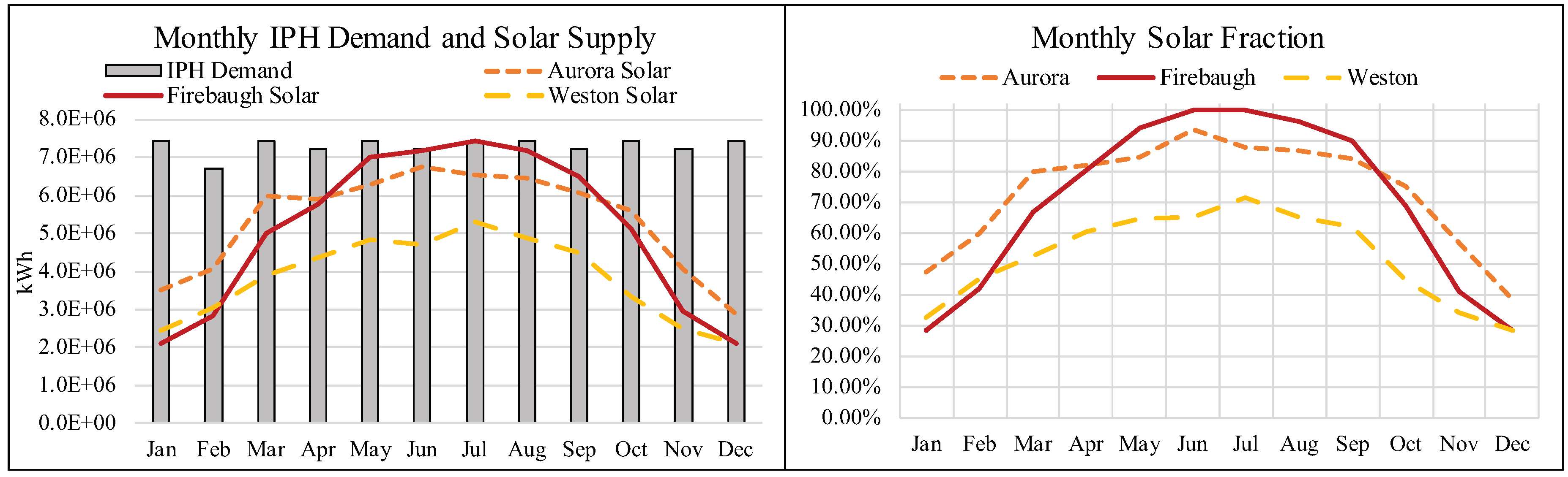
The monthly thermal performance profiles for the global optimal designs are shown in Figure 3. Both Aurora and Weston experience less seasonal variance in DNI than Firebaugh (see Table A3) and so the thermal performance profiles appear flatter over the year than those for Firebaugh. Even though the annual average DNI for Aurora and Firebaugh are within about 8% of each other, they differ by as much as 36% in the summer months. Hence, the optimal designs for Firebaugh are significantly smaller and provide significantly more lifecycle savings than those for Aurora. Interestingly, the optimal TES capacity for Weston and Firebaugh are very similar, whereas the PTC aperture area for Weston sits between Firebaugh and Aurora. Clearly, the widely differing DNI profiles has a dramatic influence on the optimal designs.
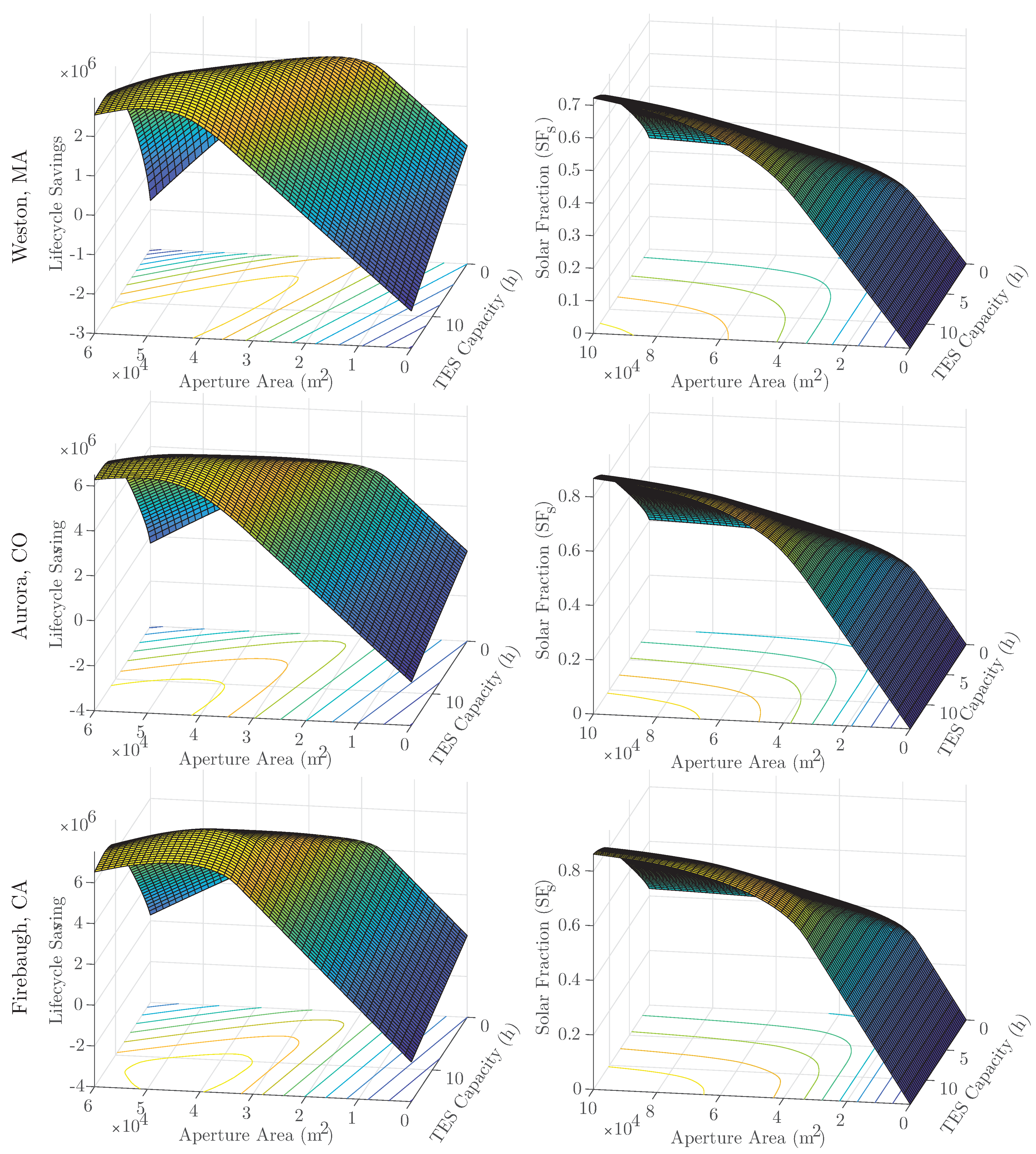
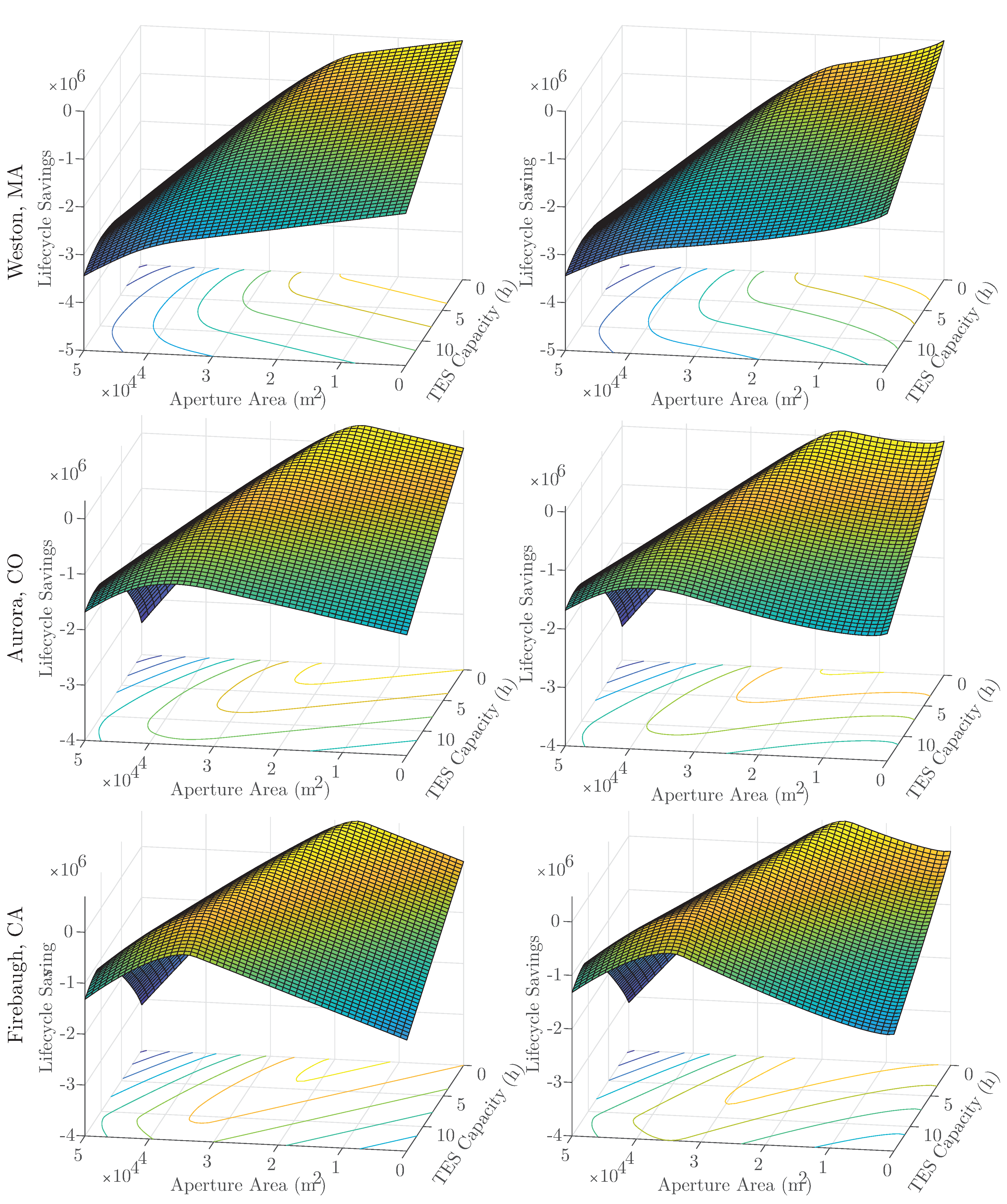
The and functions are plotted in Figure 4 for each geographic location for comparison. Each of the surfaces are qualitatively similar but there are clear differences between the geographic regions in terms of how sharply the economics change as you move away from the optimal design. The lifecycle savings for Weston are much more sensitive to the design decisions than Aurora and Firebaugh, which exhibit broader relatively-flat regions around the optimum. This explains why the optimal economics between the fixed-pricing and discount-pricing models are within less than 2% for Aurora and Firebaugh but almost 7% for Weston. It can be concluded from this analysis that designing solar-IPH hybridization strategies for lower-DNI regions may require the use of higher-accuracy cost models (e.g., discount-pricing models) with global optimization.
3.2. Periodic IPH Demand, Commercial Fuel Rate
In this study, the IPH demand is modeled using Equation (11) with kW and . Hence, this case ramps up thermal power demand by 10% over the mean at the height of the workday ( MW) and then ramps down to 10% below the mean by midnight to simulate reduced staffing and production output overnight. We consider the commercial rate for fuel [45] and we let .
Table 2 contains the location information and corresponding optimal solar-IPH hybridization strategies (i.e., the optimal solutions of Equation (19)) for both the linear fixed-pricing model in Equation (15) and the nonconvex discount-pricing model in Equation (14). As expected, the optimal designs have lower TES capacities than the constant IPH demand since the periodic demand is relatively synchronized with the sunrise and sunset. Further, the optimal PTC aperture areas are very similar to the constant IPH demand case since the total energy consumption between the two cases are the same. Note, the TES capacity is scaled against the peak IPH demand . Hence, to compare the TES capacity between the periodic IPH case and the constant IPH case, we need to scale them using , for each case. Thus, for the Weston fixed-pricing model and constant IPH demand, we have a TES capacity of 11.24 h kW=1.124 MWh. For the Weston fixed-pricing model and periodic IPH demand, we have a TES capacity of 9.537 h kW=1.05 MWh. Thus, the TES capacity is roughly 7% larger for the constant IPH demand over the periodic IPH demand. The periodic IPH demand is clearly more economical from a solar hybridization perspective. However, without accounting for the economics of the process itself, one cannot conclude that it should be operated in such a periodic fashion to achieve overall-better economics. In other words, it may be more costly to operate the process in a periodic fashion than what is saved with an optimal solar hybrid design.
3.3. Constant IPH Demand, Industrial Fuel Rate
We consider the IPH demand modeled using Equation (11) with kW and (i.e., constant demand profile). In this case, the industrial rate for fuel [45] is considered from Table A2 and we let . The objective function surfaces for both the fixed-pricing model () and discount-pricing model ( ) are plotted in Figure 5. Table 3 contains the location information and corresponding optimal solar-IPH hybridization strategies (i.e., the optimal solutions of Equation (19)) for both the linear fixed-pricing model in Equation (15) and the nonconvex discount-pricing model in Equation (14).
It is clear from Table 3 and Figure 5 that the lower fuel costs dramatically reduce the lifecycle savings, and therefore jeopardize the economic viability of the hybridization project. Further, the reduced fuel costs ensure that the capital cost terms have a much greater impact on the lifecycle savings. As a result, significant nonconvexity is observed for the discount-pricing model. In fact, for the Aurora and Firebaugh cases, there exists a suboptimal local minimum at . IPOPT was applied to the nonconvex problem directly and only found the suboptimal local minima unless the domain was manually partitioned or bounded. Hence, without the application of the B&B algorithm (Algorithm A1), one may falsely conclude that solar-IPH hybridization is not economically viable. For the Weston, MA case, the fixed-pricing model concludes that the project is not economically viable, and hence, neither is the project with the discount-pricing model due to the upper-bounding relationship in Equation (18). Similar trends in the optimal solutions for the other locations are observed as for the previous cases. However, it is worth noting that for the Aurora and Firebaugh cases, the economics between the fixed-pricing and the discount-pricing models are significant. This is because significant nonconvexity is introduced for the lower fuel cost case. Hence, one can conclude that, for this low fuel cost case, the fixed-pricing model calculated via Corollary 1 over this large of a design space will not yield sufficiently accurate results. As a result, the discount-pricing model should be used with deterministic global optimization to ensure accurate results are obtained for feasibility studies.
3.4. Periodic IPH Demand, Industrial Fuel Rate
We consider the IPH demand modeled using Equation (11) with kW and (i.e., fluctuating demand profile). In this case, the industrial rate for fuel [45] is considered from Table A2 and we let .
Table 4 contains the location information and corresponding optimal solar-IPH hybridization strategies (i.e., the optimal solutions of Equation (19)) for both the linear fixed-pricing model in Equation (15) and the nonconvex discount-pricing model in Equation (14). The results are similar to the constant IPH demand case for the industrial fuel rate. Global optimization is required to locate the global optimal solution for the discount-pricing model case. Interestingly, the optimal solar design for the periodic IPH demand case is measurably larger in PTC aperture area over the constant IPH demand case for the same industrial fuel rate. This result differs from the commercial fuel rate cases which showed nearly identical aperture sizes between the designs. The results we see here is largely due to the very low annual solar fraction and the fact that the optimal designs call for the minimum TES capacity. Hence, the periodic IPH demand enables a greater solar fraction without adding TES capacity. However, as was identified for the constant IPH demand case, the fixed-pricing model dramatically overestimates the lifecycle savings due to the large degree of nonconvexity introduced by the discount-pricing model in the lower fuel cost case. As a result, it is still recommended for this case that the discount-pricing model is used with deterministic global optimization to ensure accurate results are obtained for feasibility studies.
3.5. Computational Efficiency
The solution times for each of the numerical experiments are provided in Table 5. The computational cost trade-off of using the fixed-pricing model versus the discount-pricing model is clear. In almost all cases, using the discount-pricing model requires an order-of-magnitude longer to solve the problem than the fixed-pricing model due to nonconvexity and the need for the B&B algorithm. Despite this, the solution times for the discount-pricing model are still favorable considering the model’s scale with state variables. As previously mentioned, the Weston location with the lower industrial fuel rate (for both IPH demand profiles) yielded the result that the hybridization project would not be economically viable. As can be seen in Table 5, these are the only cases where solving the discount-pricing model requires roughly the same order of computational effort as solving the fixed-pricing model. Additionally, due to the relationship in Equation (18), one can immediately conclude from the solution of the fixed-pricing model that the project is not economically viable. Therefore, for the purposes of investment decision-making, an additional “economic feasibility” termination criterion can be added to Algorithm 1, whereby the algorithm simply terminates if the upper bound is below some threshold of economic viability. For the purposes of this optimal design problem, the optimal solution translates to not implementing any CSP, and hence, a termination criterion could also be added that identifies this case. With these termination criteria, the B&B algorithm (Algorithm 1) would be identical in solution time to the fixed-pricing model since it would terminate at the root node with the solution of economic infeasibility after solving only the upper-bounding problem. For such cases, if . Note, from Table A2, the lower bounds on the decision variables were not exactly zero, albeit very close with respect to their scale, which helps avoid some numerical round-off issues observed. Since , the results still hold.
4. Conclusions
A dynamic concentrating solar power performance model is presented for use with design optimization and investment decision-making problems for hybridizing IPH systems. The model utilizes high-fidelity solar resource data from the NSRDB [41] and accounts for the aperture area of a parabolic trough solar concentrator and the storage capacity of a thermal energy storage device as design decision variables. The solar performance model was constructed such that it is concave and differentiable on the domain of interest. Since determining the performance of the solar system requires a dynamic simulation (with 8760 time steps using hourly DNI data), concavity of the model on the decision domain ensures that it is efficient for use with mathematical optimization. Additionally, an economic model based on the lifecycle savings was constructed that utilizes the solar performance model as well as two capital cost models: a linear fixed-pricing model and a nonconvex discount-pricing model. The convex envelopes of the nonconvex discount-pricing model were presented, which, when used within a spatial Branch-and-Bound algorithm, enable the global solution of the economic optimization problem with the nonconvex discount-pricing model. For the higher-cost commercial fuel rate, optimization of the fixed-pricing model and the discount-pricing model show good agreement. However, for the lower-cost industrial fuel rate, significant nonconvexity complicates the problem and therefore the greater-accuracy discount-pricing model (and global optimization) is recommended for investment decision-making.
The economic model presented herein is relatively simple to illustrate the trade-off between the fuel savings and the capital cost of the project. Greater levels of detail can easily be incorporated in this model, such as taxes, incentives, capital depreciation, carbon pricing, detailed O&M, etc. Similarly, the solar thermal performance model assumes the simplifying characteristics of negligible heat losses, ideal temperature delivery, and negligible CST array shadowing. These details can be readily incorporated in this model, if necessary. The developed models may serve as the foundation for more greater-complexity model-building for systems performance and economic analyses. Specifically, the models may easily incorporate various sources of uncertainty and investment and/or thermal performance thresholds to address robust design and operations under uncertainty and new technology investment risk. However, if enhancing complexity, the user must consider how convexity/concavity and computational tractability are affected. For example, simple tax models and carbon pricing models may be incorporated as increased O&M costs without significantly affecting computational cost or convexity/concavity results. However, high-fidelity heat transfer models complicate the calculation of the annual solar fraction which substantially increase the integration cost and may introduce nonconvexity/nonconcavity. In this case, solving the optimization problem(s) will become extremely computationally expensive as convex and concave relaxations of must be introduced, ensuring many more iterations of the B&B algorithm are required to identify an optimal solution. Similarly, accounting for various sources of uncertainty may have equivalent effects. As additional modeling complexity may add significant computational burden, the models presented herein represent a balanced approach between computational cost and modeling complexity for the purposes of optimization problem tractability and sufficient accuracy of the results for engineering design and investment decision-making.
Funding
This research received no external funding.
Acknowledgments
Funding for this work was provided by the University of Connecticut.
Conflicts of Interest
The author declares no conflict of interest.
Abbreviations
The following abbreviations are used in this manuscript:
| B&B | Branch-and-Bound |
| CSP | Concentrating Solar Power |
| CST | Concentrating Solar Thermal |
| IPH | Industrial Process Heat |
| LCS | Lifecycle Savings |
| NLP | Nonlinear Program |
| NREL | National Renewable Energy Laboratory |
| NSRDB | National Solar Radiation Database |
| O&M | Operations and Maintenance |
| PTC | Parabolic Trough Solar Concentrator |
| TES | Thermal Energy Storage |
| TMY | Typical Meteorological Year |
Appendix A. Solar Position Model
Unless the CST technology of interest employs two-axis tracking, the center of the performance model is the incidence angle: the angle which the incoming solar radiation strikes the mirrors of the concentrator as measured from the normal of the concentrator aperture plane (see Figure 1). Since the sun’s position in the sky is well-understood to a very high-degree of accuracy for a static global position, the incidence angle is readily calculable for every moment in time. With the incidence angle and the physical design of the CST technology, the specific thermal energy output can be calculated. The incidence angle calculation follows from [25,27,29,30,50] and the calculation of the solar position as a function of time. The model is included here for clarity and completeness.
Definition A1
(Equation of Time Factors, B,ST,TC [27]). Due to the eccentricity of the Earth’s orbit and tilt of its axis, the length of a day varies throughout the year. The variation is calculated by the solar time :
with B in degrees and in minutes and the integer N as the day number. To relate the solar time to the local time, a time correction, (in minutes), is required:
where (+) is chosen if the location is east of the prime meridian and (−) if it is to the west.
Definition A2
(Declination Angle, δ [27]). The solar declination angle δ is the angular distance of the sun’s rays north (or south) of the equator:
Definition A3
(Hour Angle, γ [27]). The hour angle γ is the angle between the meridian of an observer and the sun. It is negative before local solar noon and positive after local solar noon. At local solar noon, . The hour angle (in degrees) is defined as
Definition A4
(Zenith Angle, ϕ [27]). The solar zenith angle ϕ (in degrees) is the angle between the sun’s rays and the vertical plane:
Definition A5
(Solar Elevation (Altitude) Angle, [27]). The solar elevation or altitude angle α (in degrees) is the angle between the sun’s rays and the horizontal plane:
Definition A6
(Azimuth Angle, ζ [27]). The solar azimuth angle ζ is the angle between the sun’s rays and due South for the Northern Hemisphere. If the sun rises and/or sets south of the East–West line (i.e., ), then we have:
For certain periods of the year and for certain locations, this may not be the case (i.e., ), and the azimuth angle becomes:
Definition A7
(Surface Tilt Angle, β [27]). The surface tilt angle β of a horizontal surface with a N-S axis orientation and E-W tracking is given by:
with the convention of due East and due West.
Definition A8
Note, to maximize the collection of solar energy, the incidence angle must be minimized at all times. The extent to which this angle can be minimized depends on the orientation of the collector and the tracking capability of the collector (e.g., fixed non-tracking, one-axis tracking, and two-axis tracking). Other orientations and tracking capabilities are discussed further in [27].
Appendix B

Table A1.
The PTC modeling parameters.
| , Shadowing Factor | 0.98 |
| , Tracking Error | 0.994 |
| , Geometry Error | 0.98 |
| , Mirror Dirt Factor | |
| , Glass Receiver Envelope Dirt Factor | |
| , Unaccounted Losses | 0.96 |
| , Mirror Reflectance | 0.935 |
| , Receiver Tube Absorptance | 0.94 |
| , Glass Receiver Envelope Transmittance | 0.963 |
Table A2.
The economic modeling and optimization parameters.
| , specific installed cost of PTC ($/m) | 425.0 |
| , specific installed cost of TES ($/kWh) | 45.14 |
| , commercial initial specific fuel cost ($/kWh) | 7.232/293.1≈ 0.02467 |
| industrial initial specific fuel cost ($/kWh) | 3.420/293.1≈ 0.01167 |
| r, discount rate (-) | 10% |
| , capital financing APR (-) | 6.5% |
| , fuel cost annual inflation rate (-) | 1% |
| , loan term (years) | 10 |
| , lifetime of project (years) | 30 |
| , variable lower bound (h, m) | |
| , variable upper bound (commercial fuel case) (h, m) | |
| variable upper bound (industrial fuel case) (h, m) | |
| , minimum solar fraction (-) | 0 |
Table A3.
The annual average DNI (kWh/m/day) for each location is resolved by month. The data are calculated from the hourly TMY values obtained from [41].
Table A3.
The annual average DNI (kWh/m/day) for each location is resolved by month. The data are calculated from the hourly TMY values obtained from [41].
| Month | Weston | Aurora | Firebaugh |
|---|---|---|---|
| Janary | 3.73 | 4.68 | 3.21 |
| Febrary | 4.41 | 5.25 | 4.24 |
| March | 4.61 | 6.36 | 6.07 |
| April | 5.31 | 6.42 | 7.03 |
| May | 5.33 | 6.72 | 8.68 |
| June | 5.32 | 7.98 | 10.16 |
| July | 5.60 | 7.14 | 9.54 |
| August | 5.37 | 6.82 | 9.30 |
| Sepember | 5.24 | 7.21 | 7.70 |
| Octorber | 4.13 | 6.33 | 6.54 |
| November | 3.72 | 5.44 | 4.50 |
| December | 3.39 | 4.08 | 3.36 |
| Ann. Avg. | 4.68 | 6.21 | 6.71 |
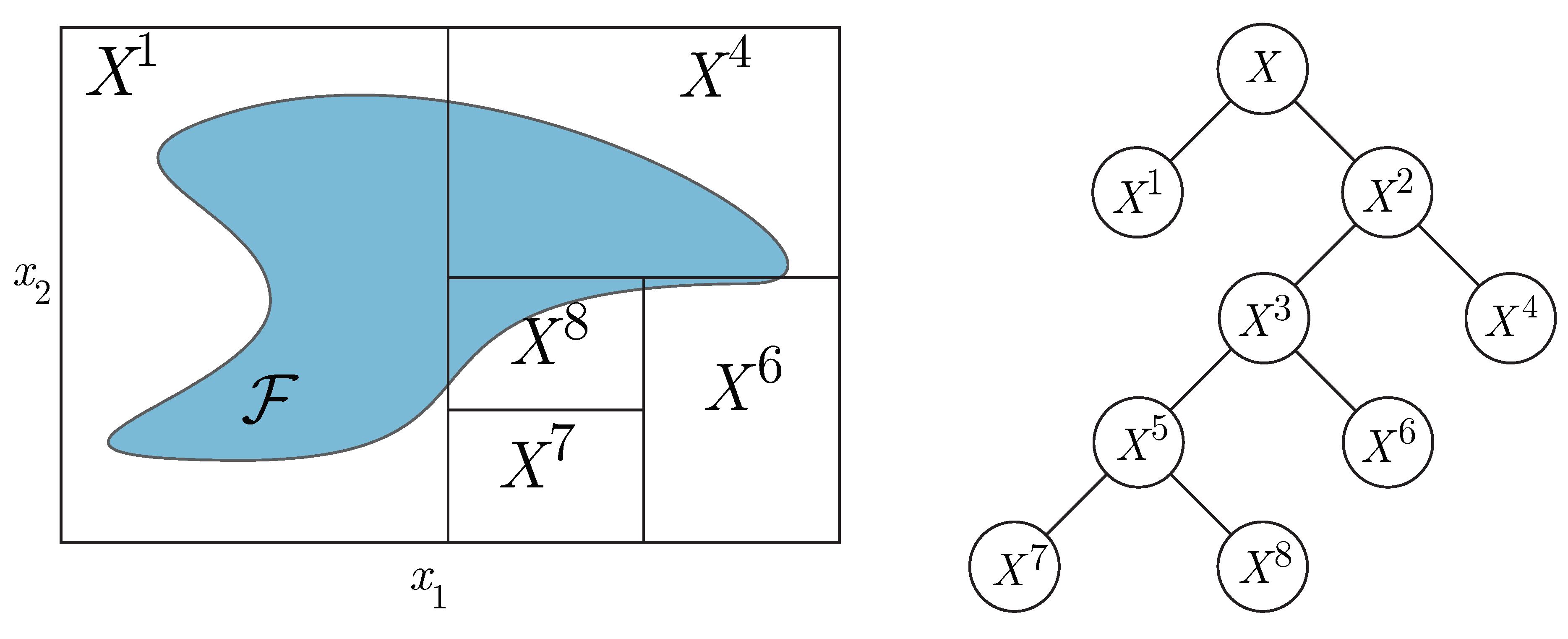
Appendix C. Spatial Branch-and-Bound (B&B) Global Optimization
The spatial B&B algorithm is a deterministic global optimization algorithm that is guaranteed to find a global optimum (within some numerical tolerance ) of a nonlinear program or determine that the problem is infeasible in finitely-many iterations. The algorithm systematically partitions the decision space X, with a procedure referred to as branching. Then, upper- and lower-bounds on the global optima on each partition of X are obtained by solving corresponding optimization problems (or interval analysis calculations). A summary of the algorithm is provided here for solving maximization problems as in Equation (19). Here, we present the B&B algorithm (Algorithm 1) for solving Equation (19) with to global optimality. The upper- and lower-bounding problems are defined in Equations (A1) and (A2), respectively. The concept of partitioning the decision space X is illustrated in Figure A1.
Definition A9
(Upper-Bounding Problem). Consider an interval . The upper-bounding problem is given by:
Definition A10
(Lower-Bounding Problem). Consider an interval . The lower-bounding problem is given by:
Figure A1.
(Left) The decision space X (outer box) is shown overlaying the feasible set and is partitioned into subintervals using a bisection strategy. Note that and therefore the corresponding upper- and lower-bounding problems are infeasible. (Right) An illustration of the B&B tree corresponding to the decision space partitioning.

| Algorithm 1: Branch & Bound Maximization |
 |
References
- US Energy Information Administration. Annual Energy Outlook 2018 with Projections to 2050; Technical Report for US Department of Energy; US Energy Information Administration: Washington, DC, USA, 2018.
- US Department of Energy. Available online: https://www.energy.gov/eere/amo/dynamic-manufacturing-energy-sankey-tool-2010-units-trillion-btu (accessed on 15 May 2018).
- Kurup, P.; Turchi, C. Initial Investigation into the Potential of CSP Industrial Process Heat for the Southwest United States; Technical Report of NREL; National Renewable Energy Laboratory: Golden, Colorado, 2015.
- Farjana, S.H.; Huda, N.; Mahmud, M.P.; Saidur, R. Solar process heat in industrial systems–A global review. Renew. Sustain. Energy Rev. 2018, 82, 2270–2286. [Google Scholar] [CrossRef]
- Kalogirou, S. The potential of solar industrial process heat applications. Appl. Energy 2003, 76, 337–361. [Google Scholar] [CrossRef]
- Lauterbach, C.; Schmitt, B.; Jordan, U.; Vajen, K. The potential of solar heat for industrial processes in Germany. Renew. Sustain. Energy Rev. 2012, 16, 5121–5130. [Google Scholar] [CrossRef]
- Mekhilef, S.; Saidur, R.; Safari, A. A review on solar energy use in industries. Renew. Sustain. Energy Rev. 2011, 15, 1777–1790. [Google Scholar] [CrossRef]
- Martinez, V.; Pujol, R.; Moia, A. Assessment of Medium Temperature Collectors for Process Heat. Energy Proc. 2012, 30, 745–754. [Google Scholar] [CrossRef]
- Sharma, A.K.; Sharma, C.; Mullick, S.C.; Kandpal, T.C. Solar industrial process heating: A review. Renew. Sustain. Energy Rev. 2017, 78, 124–137. [Google Scholar] [CrossRef]
- Panwar, N.L.; Kaushik, S.C.; Kothari, S. Role of renewable energy sources in environmental protection: A review. Renew. Sustain. Energy Rev. 2011, 15, 1513–1524. [Google Scholar] [CrossRef]
- Ramos, C.; Ramirez, R.; Beltran, J. Potential Assessment in Mexico for Solar Process Heat Applications in Food and Textile Industries. Energy Proc. 2014, 49, 1879–1884. [Google Scholar] [CrossRef]
- Murray, J. Aluminum Production Using High-Temperature Solar Process Heat. Sol. Energy 1999, 66, 133–142. [Google Scholar] [CrossRef]
- Hockaday, S.; Dinter, F.; Harms, T. Opportunities for concentrated solar thermal heat in the minerals processing industry. In Proceedings of the 4th Southern African Solar Energy Conference (SASEC) 2016, Stellenbosch, South Africa, 31 October–2 November 2016. [Google Scholar]
- Mekhilef, S.; Faramarzi, S.Z.; Saidur, R.; Salam, Z. The application of solar technologies for sustainable development of agricultural sector. Renew. Sustain. Energy Rev. 2013, 18, 583–594. [Google Scholar] [CrossRef]
- Hussain, M.I.; Lee, G.H. Utilization of Solar Energy in Agricultural Machinery Engineering: A Review. J. Biosyst. Eng. 2015, 40, 186–192. [Google Scholar] [CrossRef] [Green Version]
- Beesing, M.E. Textile Drying Using Solar Process Steam. In Proceedings of the Energy Conference ASME 1979 International Gas Turbine Conference and Exhibit and Solar, San Diego, CA, USA, 12–15 March 1979. [Google Scholar] [CrossRef]
- Sharma, A.K.; Sharma, C.; Mullick, S.C.; Kandpal, T.C. GHG mitigation potential of solar industrial process heating in producing cotton based textiles in India. J. Clean. Prod. 2017, 145, 74–84. [Google Scholar] [CrossRef]
- Sharma, A.K.; Sharma, C.; Mullick, S.C.; Kandpal, T.C. Incentives for promotion of solar industrial process heating in India: a case of cotton-based textile industry. Clean Technol. Environ. Policy 2018, 20, 813–823. [Google Scholar] [CrossRef]
- Frey, P.; Fischer, S.; Drück, H.; Jakob, K. Monitoring Results of a Solar Process Heat System Installed at a Textile Company in Southern Germany. Energy Proc 2015, 70, 615–620. [Google Scholar] [CrossRef]
- Sharma, A.K.; Sharma, C.; Mullick, S.C.; Kandpal, T.C. Potential of Solar Energy Utilization for Process Heating in Paper Industry in India: A Preliminary Assessment. Energy Proc. 2015, 79, 284–289. [Google Scholar] [CrossRef]
- Sharma, A.K.; Sharma, C.; Mullick, S.C.; Kandpal, T.C. Carbon mitigation potential of solar industrial process heating: paper industry in India. J. Clean. Prod. 2016, 112, 1683–1691. [Google Scholar] [CrossRef]
- Meier, A.; Bonaldi, E.; Cella, G.M.; Lipinski, W.; Wuillemin, D. Solar chemical reactor technology for industrial production of lime. Sol. Energy 2006, 80, 1355–1362. [Google Scholar] [CrossRef]
- Romero, M.; Steinfeld, A. Concentrating solar thermal power and thermochemical fuels. Energy Environ. Sci. 2012, 5, 9234–9245. [Google Scholar] [CrossRef]
- Kalogirou, S.; Lloyd, S.; Ward, J. Modelling, optimisation and performance evaluation of a parabolic trough solar collector steam generation system. Sol. Energy 1997, 60, 49–59. [Google Scholar] [CrossRef]
- Duffie, J.A.; Beckman, W.A. Solar Engineering of Thermal Processes; John Wiley & Sons: Hoboken, NJ, USA, 2013. [Google Scholar]
- Kalogirou, S.A. A detailed thermal model of a parabolic trough collector receiver. Energy 2012, 48, 298–306. [Google Scholar] [CrossRef]
- Kalogirou, S.A. Solar Energy Engineering Processes and Systems, 2nd ed.; Academic Press: Oxford, UK, 2014. [Google Scholar]
- Ghobeity, A.; Mitsos, A. Optimal design and operation of a solar energy receiver and storage. J. Sol. Energy Eng. 2012, 134. [Google Scholar] [CrossRef]
- Ghasemi, H.; Sheu, E.; Tizzanini, A.; Paci, M.; Mitsos, A. Hybrid solar-geothermal power generation: Optimal retrofitting. Appl. Energy 2014, 131, 158–170. [Google Scholar] [CrossRef]
- Gunasekaran, S.; Mancini, N.; El-Khaja, R.; Sheu, E.; Mitsos, A. Solar-geothermal hybridization of advanced zero emissions power cycle. Energy 2014, 65, 152–165. [Google Scholar] [CrossRef]
- Silva, R.; Berenguel, M.; Perez, M.; Fernandez-Garcia, A. Thermo-Economic Design Optimization of Parabolic Trough Solar Plants for Industrial Process Heat Applications with Memetic Algorithms. Appl. Energy 2014, 113, 603–614. [Google Scholar] [CrossRef]
- Stuber, M.D. Optimal Design of Fossil-Solar Hybrid Thermal Desalination for Saline Agricultural Drainage Water Reuse. Renew. Energy 2016, 89, 552–563. [Google Scholar] [CrossRef]
- Yan, C.; Wang, S.; Ma, Z.; Shi, W. A simplified method for optimal design of solar water heating systems based on life-cycle energy analysis. Renew. Energy 2015, 74, 271–278. [Google Scholar] [CrossRef]
- Baniassadi, A.; Momen, M.; Amidpour, M. A new method for optimization of Solar Heat Integration and solar fraction targeting in low temperature process industries. Energy 2015, 90, 1674–1681. [Google Scholar] [CrossRef]
- Frasquet, M. SHIPcal: Solar heat for industrial processes online calculator. Energy Proc. 2016, 91, 611–619. [Google Scholar] [CrossRef]
- Ayub, M.; Mitsos, A.; Ghasemi, H. Thermo-economic analysis of a hybrid solar-binary geothermal power plant. Energy 2015, 87, 326–335. [Google Scholar] [CrossRef]
- Al-Aboosi, F.Y.; El-Halwagi, M.M. An Integrated Approach to Water-Energy Nexus in Shale-Gas Production. Processes 2018, 6, 52. [Google Scholar] [CrossRef]
- Stuber, M.D.; Sullivan, C.; Kirk, S.A.; Farrand, J.A.; Schillaci, P.V.; Fojtasek, B.D.; Mandell, A.H. Pilot demonstration of concentrated solar-powered desalination of subsurface agricultural drainage water and other brackish groundwater sources. Desalination 2015, 355, 186–196. [Google Scholar] [CrossRef]
- Dudley, V.E.; Kolb, G.J.; Mahoney, A.R.; Mancini, T.R.; Matthews, C.W.; Sloan, M.; Kearney, D. Test Results: SEGS LS-2 Solar Collector; Technical Report of Sandia National Labs.; National Technical Information Service: Albuquerque, NM, USA, 1994.
- Forristall, R. Heat Transfer Analysis and Modeling of a Parabolic Trough Solar Receiver Implemented in Engineering Equation Solver; Technical Report of NREL; National Renewable Energy Laboratory: Golden, CO, USA, 2003.
- National Renewable Energy Laboratory. NSRDB: National Solar Radiation Database. Available online: https://nsrdb.nrel.gov/nsrdb-viewer (accessed on 21 May 2018).
- International Renewable Energy Agency. Renewable Energy Technologies: Cost Analysis Seris—Concentrating Solar Power; Technical Report of IRENA; International Renewable Energy Agency: Abu Dhabi, UAE, 2012. [Google Scholar]
- Falk, J.E.; Soland, R.M. An Algorithm for Separable Nonconvex Programming Problems. Manag. Sci. 1969, 15, 550–569. [Google Scholar] [CrossRef]
- Bezanson, J.; Edelman, A.; Karpinski, S.; Shah, V.B. Julia: A Fresh Approach to Numerical Computing. SIAM Rev. 2017, 59, 65–98. [Google Scholar] [CrossRef] [Green Version]
- US Energy Information Administration. Available online: https://www.eia.gov/dnav/ng/NG_PRI_SUM_DCU_NUS_M.htm (accessed on 16 April 2018).
- Wächter, A.; Biegler, L.T. On the implementation of an interior-point filter line-search algorithm for large-scale nonlinear Programming. Math. Program. 2006, 106, 25–57. [Google Scholar] [CrossRef]
- Dunning, I.; Huchette, J.; Lubin, M. JuMP: A modeling language for mathematical optimization. SIAM Rev. 2017, 59, 295–320. [Google Scholar] [CrossRef]
- Wilhelm, M.; Stuber, M.D. Easy Advanced Global Optimization (EAGO): An Open-Source Platform for Robust and Global Optimization in Julia. In Proceedings of the AIChE Annual Meeting 2017 Minneapolis, Minneapolis, MN, USA, 31 October 2017. [Google Scholar]
- Wilhelm, M.; Stuber, M.D. EAGO: Easy Advanced Global Optimization Julia Package. Available online: https://github.com/PSORLab/EAGO.jl (accessed on 1 May 2018).
- Kreith, F.; Kreider, J.F. Principles of Solar Engineering; Hemisphere Publishing Corporation: Washington, DC, USA, 1978. [Google Scholar]
Figure 1.
(left) An illustration of a parabolic trough solar concentrator (PTC) with the defined array length , aperture length and the aperture plane with incident solar radiation. (right) The large-aperture PTC (Skyfuel, Lakewood, CO, USA) powering a solar thermal desalination pilot by Stuber et al. [38].

Figure 2.
The block-flow diagram representation of the hybrid solar industrial process heat system being modeled.
Figure 2.
The block-flow diagram representation of the hybrid solar industrial process heat system being modeled.

Figure 3.
The thermal performance of the global optimal hybridization strategies for constant IPH demand and the commercial initial specific fuel cost.
Figure 3.
The thermal performance of the global optimal hybridization strategies for constant IPH demand and the commercial initial specific fuel cost.

Figure 4.
The objective function surfaces (left column) and the solar fraction surfaces (right column) for constant IPH demand for commercial fuel rate show similar qualitative trends between each region (rows).
Figure 4.
The objective function surfaces (left column) and the solar fraction surfaces (right column) for constant IPH demand for commercial fuel rate show similar qualitative trends between each region (rows).

Figure 5.
The objective function surfaces (left column) and (right column) for constant IPH demand for industrial fuel rates are plotted for each geographic location. The discount-pricing model exhibits nonconvexity in all cases and suboptimal local minima for Aurora and Firebaugh.
Figure 5.
The objective function surfaces (left column) and (right column) for constant IPH demand for industrial fuel rates are plotted for each geographic location. The discount-pricing model exhibits nonconvexity in all cases and suboptimal local minima for Aurora and Firebaugh.

Table 1.
The optimal solar-IPH hybridization strategies for the three geographic locations for constant IPH demand with kW for the commercial fuel rate. The global optimal results for the concave capital cost model in Equation (14) are included for comparison against the linear capital cost model in Equation (15).
| City, State | Lat., Long. | Time Zone | Capital Model | (h) | (m) | ||
|---|---|---|---|---|---|---|---|
| Weston, MA | 42.37,−71.30 | −5 | (Linear), Equation (15) | 11.24 | 46,436.4 | 0.516 | $2.976 M |
| (Concave), Equation (14) | 11.72 | 48,229.1 | 0.523 | $2.795 M | |||
| Aurora, CO | 39.73,−104.66 | −7 | (Linear), Equation (15) | 13.85 | 50,618.1 | 0.721 | $6.487 M |
| (Concave), Equation (14) | 14.58 | 53,238.5 | 0.731 | $6.377 M | |||
| Firebaugh, CA | 36.85,−120.46 | −8 | (Linear), Equation (15) | 11.42 | 42,601.7 | 0.695 | $7.533 M |
| (Concave), Equation (14) | 11.72 | 43,615.2 | 0.698 | $7.320 M |
Table 2.
The optimal solar-IPH hybridization strategies for the three geographic locations for periodic IPH demand with kW and for the commercial fuel rate. The global optimal results for the concave capital cost model in Equation (14) are included for comparison against the linear capital cost model in Equation (15).
| City, State | Lat., Long. | Time Zone | Capital Model | (h) | (m) | ||
|---|---|---|---|---|---|---|---|
| Weston, MA | 42.37,−71.30 | −5 | (Linear), Equation (15) | 9.537 | 46,248.8 | 0.507 | $3.079 M |
| (Concave), Equation (14) | 9.966 | 47,945.8 | 0.521 | $2.881M | |||
| Aurora, CO | 39.73,−104.66 | −7 | (Linear), Equation (15) | 11.92 | 50,006.8 | 0.706 | $6.593 M |
| (Concave), Equation (14) | 12.59 | 53,238.7 | 0.731 | $6.460 M | |||
| Firebaugh, CA | 36.85,−120.46 | −8 | (Linear), Equation (15) | 9.732 | 42,688.4 | 0.691 | $7.641 M |
| (Concave), Equation (14) | 9.966 | 43,615.2 | 0.698 | $7.411 M |
Table 3.
The optimal solar-IPH hybridization strategies for the three geographic locations for constant IPH demand with kW for the industrial fuel rate. The global optimal results for the concave capital cost model in Equation (14) are included for comparison against the linear capital cost model in Equation (15).
| City, State | Lat., Long. | Time Zone | Capital Model | (h) | (m) | ||
|---|---|---|---|---|---|---|---|
| Weston, MA | 42.37,−71.30 | −5 | (Linear), Equation (15) | 0.001 | 0.01 | 0.000 | $920.2 |
| (Concave), Equation (14) | 0.001 | 0.01 | 0.000 | $920.2 | |||
| Aurora, CO | 39.73,−104.66 | −7 | (Linear), Equation (15) | 0.001 | 15,720.7 | 0.250 | $323.8 k |
| (Concave), Equation (14) | 0.001 | 15,648.7 | 0.248 | $95.59 k | |||
| Firebaugh, CA | 36.85,−120.46 | −8 | (Linear), Equation (15) | 0.046 | 16,581.5 | 0.298 | $698.1 k |
| (Concave), Equation (14) | 0.001 | 16,424.3 | 0.295 | $468.3 k |
Table 4.
The optimal solar-IPH hybridization strategies for the three geographic locations for periodic IPH demand with kW for the industrial fuel rate. The global optimal results for the concave capital cost model in Equation (14) are included for comparison against the linear capital cost model in Equation (15).
| City, State | Lat., Long. | Time Zone | Capital Model | (h) | (m) | ||
|---|---|---|---|---|---|---|---|
| Weston, MA | 42.37,−71.30 | −5 | (Linear), Equation (15) | 0.001 | 0.01 | 0.000 | $773.4 |
| (Concave), Equation (14) | 0.001 | 0.01 | 0.000 | $773.4 | |||
| Aurora, CO | 39.73,−104.66 | −7 | (Linear), Equation (15) | 0.001 | 16,894.0 | 0.267 | $350.2 k |
| (Concave), Equation (14) | 0.001 | 16,879.1 | 0.267 | $120.8 k | |||
| Firebaugh, CA | 36.85,−120.46 | −8 | (Linear), Equation (15) | 0.033 | 17,972.1 | 0.320 | $759.4 k |
| (Concave), Equation (14) | 0.001 | 17,839.1 | 0.318 | $529.4 k |
Table 5.
The solution times (in seconds) for each of the numerical experiments.
| City, State | Section 3.1 | Section 3.2 | Section 3.3 | Section 3.4 | ||||
|---|---|---|---|---|---|---|---|---|
| Weston, MA | 1.09 | 10.4 | 0.632 | 13.3 | 0.103 | 0.42 | 0.103 | 0.39 |
| Aurora, CO | 0.70 | 6.69 | 0.495 | 6.40 | 0.187 | 15.5 | 0.208 | 19.4 |
| Firebaugh, CA | 0.70 | 10.1 | 1.06 | 9.92 | 0.604 | 12.77 | 0.517 | 12.67 |
© 2018 by the author. Licensee MDPI, Basel, Switzerland. This article is an open access article distributed under the terms and conditions of the Creative Commons Attribution (CC BY) license (http://creativecommons.org/licenses/by/4.0/).
Share and Cite
MDPI and ACS Style
Stuber, M.D. A Differentiable Model for Optimizing Hybridization of Industrial Process Heat Systems with Concentrating Solar Thermal Power. Processes 2018, 6, 76. https://doi.org/10.3390/pr6070076
AMA Style
Stuber MD. A Differentiable Model for Optimizing Hybridization of Industrial Process Heat Systems with Concentrating Solar Thermal Power. Processes. 2018; 6(7):76. https://doi.org/10.3390/pr6070076
Chicago/Turabian StyleStuber, Matthew D. 2018. "A Differentiable Model for Optimizing Hybridization of Industrial Process Heat Systems with Concentrating Solar Thermal Power" Processes 6, no. 7: 76. https://doi.org/10.3390/pr6070076
Note that from the first issue of 2016, this journal uses article numbers instead of page numbers. See further details here.