An Adaptive Approach Based on Resource-Awareness Towards Power-Efficient Real-Time Periodic Task Modeling on Embedded IoT Devices

Abstract

Embedded devices are gaining popularity day by day due to the expanded use of Internet of Things applications. However, these embedded devices have limited capabilities concerning power and memory. Thus, the applications need to be tailored in such a way to perform the specified tasks within the constrained resources with the same accuracy. In Real-Time task scheduling, one of the challenging factors is the intelligent modelling of input tasks in such a way that it produces not only logically correct output within the deadline but also consumes minimum CPU power. Algorithms like Rate Monotonic and Earliest Deadline First compute hyper-period of input tasks for periodic repetition of the same set of tasks on CPU. However, at times when the tasks are not adequately modelled, they lead to an enormously high value of hyper-period which result in more CPU cycles and power consumption. Many state-of-the-art solutions are presented in this regard, but the main problem is that they limit tasks from having all possible period values; however, with the vision of Industry 4.0, where most of the tasks will be doing some critical manufacturing activities, it is highly discouraged to prevent them of a certain period. In this paper, we present a resource-aware approach to minimise the hyper-period of input tasks based on device profiles and allows tasks of every possible period value to admit. The proposed work is compared with similar existing techniques, and results indicate significant improvements regarding power consumptions.

1. Introduction

With the rapid revolution of organisations from the physical space to a cyber world [1], the concept of the Internet of Things (IoT) is earning further acclaim as the cyber world demands interconnecting things via IoT [2,3,4]. In order to enhance the system efficiency and make them more affordable, technologies like Radio Frequency Identification (RFID), Barcodes and Quick Response (QR) codes have been in use for physical object identification. Likewise, Wireless Sensor Networks (WSNs), Wireless Mesh Networks, Wireless LAN (WLAN), Mobile Networks and Internet have been employed to make them reachable [5,6,7,8,9]. Physical objects connecting networks and the real world, act as edge-nodes for IoT, sensing ambient states and attaching themselves to the IoT [10]. The exchanges among IoT edge-nodes happen in real time on embedded hardware; these devices have limited capabilities in terms of power, memory, and speed, thus consequently brings difficulties for sustaining real-time requirements of these systems [11,12].

A more recent advancement in the field of IoT is the vision of Industry 4.0. In Germany, this becomes a buzzword since its inception. In this paradigm, the concept of smart factories is introduced by automating the real-time manufacturing process and mass customisation of the products [13]. The convergence of Industry 4.0 and IoT applications gives rise to another field of research known as a Cyber-Physical System (CPS). Real-time IoT and CPS extend the traditional concept of IoT by further interjecting timeliness in every perspective. In reality, real-time IoT and CPS suggest the coupling and coordination between computational and physical entities in real time. These applications are generally closed-loop control applications such as Industry 4.0 and thus demand end-to-end latency thresholds, which can be served by analysing every aspect of the wireless networks, constraint tasks scheduling, real-time cloud service, real-time data analytics, and so on. Consequently, it has become crucial how we can design real-time IoT and CPS that can satisfy the end-to-end real-time performance. Real-time processes are referred to as those whose accuracy of the program not only depends on the logically correct outcome of computations but also depends on the time consumed for the correct outcome [14,15]. Real-time systems exist in almost in every field, such as command and control systems and process control systems that can be in any domain depending on scenarios. Some other examples of real-time systems are flight control systems, defence systems and space shuttle avionics systems. The main drawback of real-time systems can be their dependence on the coming events’ knowledge that increases the cost and makes them inflexible to uncertain situations. In the coming ages, a true real-time system should be a hard real-time system, which meets the design goal of Industry 4.0 and Cyber-Physical Systems [16].

When activities have timing constraints, scheduling them in a such a way to meet their timing constraints is one major problem that comes to mind. Two primary categories of algorithms, namely static priority and dynamic priority, are suggested in the literature for traditional real-time systems. In the more recent past, progress has been made on the analysis of these real-time algorithms under the context of IoT, where the tasks need to be run on physical embedded devices. Research in the scheduling area for embedded systems can be leveraged in the context of IoT applications, but most of the algorithms that run well on general purpose systems do not scale well on these embedded devices because of their limited capabilities in terms of power and energy management. This issue becomes even more challenging for the periodic real-time tasks. Periodic real-time tasks are those tasks that repeat themselves after a certain time interval known as the period. The period plays a pivotal role in the overall system’s performance and is regarded as an optimisation variable in many studies. Algorithms like Rate Monotonic (RM) [17], Earliest Deadline First (EDF) [18] and Deadlock Monotonic (DM) are among the most commonly used scheduling algorithms that also suffer from this period problem. These algorithms use a hyper-period to compute how much CPU clock cycles a given task set consumes and hence the power and energy consumption of these algorithms is dependent solely on the hyper-period of the real-time input tasks. In some scenarios, where periods of input tasks are not adequately modelled. For example, when all periods are prime numbers, they lead to enormously high hyper-periods despite the fact that the algorithm correctly schedules the tasks theoretically, but devices don’t have sufficient resources to deal with such a high hyper-period.

Some of the conventional approaches to limit the value of a hyper-period are bounded hyper-period and harmonization. In a bounded hyper-period approach [19], a static threshold is fixed, and the hyper-period is limited below this static threshold. In a harmonization approach [20,21], though no such threshold is defined, the period values are in harmonic series and thus one value of a period will be the harmonic factor of another. The RM algorithm gives 100% utilization for a harmonic period. Both of these approaches minimise the value of hyper-period to a great extent but have their shortcomings. The static threshold does not scale well for dynamic scenarios like IoT where the resources are not fixed, and new IoT resources can register on the fly. The harmonization approach does not allow tasks to have a period value which could contribute to the high value of the hyper-period. Consequently, it dramatically decreases the tasks’ acceptance ratio and, additionally, it is not a scalable approach that is considered a highly important attribute in the context of IoT applications.

To cope with the above-mentioned shortcomings, we propose a systematic approach that models the periods of input tasks in such a manner that it always produces a hyper-period within an optimal threshold. It overcomes the problem of high power consumption that arises due to a high hyper-period. The optimal threshold is computed based on the profiles of IoT devices and the number of IoT resources connected to them. It is a safe bound by which a system can schedule tasks without any performance degradation. Moreover, this approach allows every possible value of the period within a specific bound unlike the traditional approach of harmonization. This method is general in the sense that it covers general priority-driven systems including both fixed-priority systems and dynamic-priority systems and all those algorithms that deal with a hyper-period to schedule input tasks on CPU. The proposed algorithm is compared with state-of-the-art technologies discussed earlier, and the results are found to be making significant improvements in terms of power, memory, scalability and tasks’ acceptance rate. RM is considered as a fixed-priority algorithm, and EDF is taken as a dynamic-priority system to prove the claim that the proposed approach is generic and works well for both kinds of priority systems.

The rest of the paper is organised as follows. Section 2 describes the related work in detail. Section 3 illustrates the system model assumed and outlines the notations used throughout the text. Section 4 describes the proposed work and carries out the complexity analysis of the proposed algorithms. Section 5 presents the interaction model and details the sequence of operations among different components. Section 6 outlines the implementation setup and briefly explains the underlying tools and technologies being used. Section 7 presents experimental results in terms of many performance measures and comparison with state-of-the-art technologies that is carried out to signify the contribution of this work. Finally, Section 8 concludes the paper and gives directions for future research.

2. Related Work

Real-time IoT systems also commonly known as RT-IoT [22]. At their core, RT-IoT often intersects with traditional real-time systems and modern CPS. In RT-IoT, the embedded devices are controlled remotely and thus enable conventional real-time systems to be controlled remotely. In recent years, the scope of real-time systems has been broadened, and numerous real-time applications and frameworks have been proposed for IoT and CPS systems to remotely control and schedule real-time jobs [23,24,25]. Scheduling problem on IoT has lately attracted many researchers, and notable efforts have been put forward in this regard. Much like in traditional real-time systems, in IoT, one primary issue is how to deal with constrained devices and design context-aware strategies [26,27]. Techniques like “Normally-off” sensors are proposed to limit the power consumption of IoT devices by activating sensors only on specific events. When sensors finished performing designated tasks, they are turned off to control the power they consume in idle state [26]. Likewise, in a more recent work, an energy-efficient packet scheduling is proposed for IoT application [27]. Energy and power are often portrayed as an optimisation variable, and different scheduling techniques are applied to minimise these variables.

The analysis of power-consumption in embedded devices has been vital in general real-time systems and modern RT-IoT systems. Vivek et al. [28] first analysed the correlation between power and energy, and claimed that power and energy consumption of embedded devices is a function of CPU clock cycles. Therefore, the focus of the later researchers was to design scheduling strategies which consume less CPU clock cycles and hence less power and energy. One primary driver for high CPU clock-cycles is the poor design of periods of input tasks which lead to a high value of hyper-period. Therefore, the hyper-period optimisation is the focus of many researchers to optimise the power and energy [20,21,29]. As discussed that a high value of hyper-period is produced due to the poor design of tasks’ periods, therefore, the period is considered a key parameter in the design of the input tasks for real-time systems. The design period was initially considered as an optimisation problem [30]. In such formulations, the performance of the system is captured through an exponentially decreasing function. Furthermore, the period is modelled as an optimisation variable that can have any values within a certain feasible range to ensure the schedulability of the system. In scheduling theory, there are two broad categories of systems, dynamic-priority and static-priority. RM algorithm is based on static-priority and computes the priority of an input task based on its period. The smaller the period will be, the higher will be the priority and vice versa. On the other hand, the EDF is a dynamic-priority algorithm in which the priority of the input task dynamically changes as the scheduling advances. To choose the optimal period for given task sets, Seto et al. [31] proposed an algorithm that makes use of scheduling methods based on fixed priority. This algorithm serves as the foundation for many other algorithms, and several researchers have extended this algorithm to improve its performance. Ref. [32] have considered the stability radius as the critical performance criteria and they have developed an algorithm for assigning optimal period to the tasks, i.e., state feedback controllers. Wu et al. [33] presented a scheme based on feasibility constraints to select given tasks’ deadlines and periods. Multiple tasks having overlapping execution time will result in a conflict that is addressed through formulation for an optimisation problem by proposing a convex approximation scheme based on deadline space of EDF. Bini et al. [34] developed an algorithm based on a searching scheme in which tasks are activated using fixed priorities in a way that shall result in system performance gain without violation of the system deadline constraints.

The above-mentioned methods of the scheduling and manual input task design are employed for offline utilization only. To further improve the system robustness and flexibility, research studies are conducted to shift the optimisation algorithms from offline scenarios to more complex online applications. Du et al. [35] have developed an online algorithm based on an analytical solution using Lagrange multipliers to obtain schedulability conditions for the given optimisation problem. Using the estimated information regarding current state and noise conditions, Cervin et al. [36] developed an online algorithm for adjustment of sampling periods. In their proposed algorithm, they tried to capture the relationship among computational cost, noise factor and expected cost over finite horizon of the sampling period. They have developed an integrated scheme for detecting when the system is overloaded. The time complexity of their proposed system is deterministic, and thus the proposed method is appropriate for online applications. More recently, Cha et al. [37] developed a searching-based heuristic scheme to compute near-optimal values for feasible task periods such that the overall performance of the system is maximised. The time complexity of their proposed algorithm is linear and hence suitable for online use.

Period selection is a challenging problem, which is not only widely explored in the literature related to control systems, but also studied in applications related to general real-time systems. One of the most common methods used for the assigning period is the one based on harmonic periods of tasks. It has been proved experimentally that 100% CPU utilization can be achieved by the RM algorithm via harmonic period assignment [38]. Furthermore, the benefit of using a harmonic period for tasks is that it also results in smaller values for hyper-periods, which is highly desirable. The hyper-period is computed by calculating the Least Common Multiple (LCM) value of the selected periods of given tasks. A lower hyper-period is very important because it is the time interval in which the complete schedule is executed once, and then it repeats itself after each hyper-period of time. Analysis of the scheduling algorithm is usually carried out by executing the tasks’ sets until one hyper-period is completed and afterwards the results will be the same as the schedule will repeat itself. Therefore, a smaller hyper-period will result in overall less execution time and memory footprint due to a reduced scheduling table.

As discussed in Section 1, Nasri et al. [20,21] developed a model to capture the harmonic relationship between the period ranges. After calculating a harmonic sub-interval within the range of feasible periods for a given tasks’ set, a harmonic period can easily be computed and assigned. To further reduce the hyper-period value for resultant harmonic period assignment, Xu [39] developed a scheme based on a small adjustment in resultant periods of the given tasks. Adjusted periods of the task may not be exactly harmonic but are closely related, thus making it easy to compute the whole schedule before run time for ultimate periodic task scheduling.

Similarly, while computing periods for a given tasks’ set, different approaches for reducing the hyper-period are presented in [29,40]. However, the underlying assumption for the validity of such research is that given tasks are executed over a uni-processor platform independently. However, in a real-world environment, tasks often exhibit an interactive relationship among themselves in different forms, e.g., producer–consumer relationship [41]. Gerber et al. conducted a research study by developing a system model in which asynchronous channels are used to connect the tasks to express their relationships [42]. In their proposed system, external input and output serve as system end-points, and the whole system is then rendered in the form of asynchronous task-graph. End-to-end constraints on timing are imposed over systems’ end-points and tasks’ periods are computed accordingly.

All of the above works focus on the period optimisation in a way to get a lower value of hyper-period and hence decrease the power consumption. However, none of the above proposals identified an approach that encourages maximum possible values of the period and avoids discretisation of periods of input tasks. This discretisation and harmonization work well in the general real-time system, but, in more dynamic and modern real-time IoT systems and Industry 4.0, it may not adapt well due to a massive number of diverse task sets. This paper, to the best of the authors’ knowledge, is the first attempt to address this issue in the context of RT-IoT and Industry 4.0.

3. RT-IoT System Model

The primary driver towards RT-IoT is the controlling and monitoring of real-time embedded devices via the Internet. It enables real-time systems to be employed in a more broader domain; however, it also poses additional risks of various challenges due to the remote controlling and dependence on networks. The principal features for a typical RT-IoT are the intersection of the features of traditional real-time systems and IoT systems. In addition to that, several features are highlighted to be more distinguished for RT-IoT systems [22]:

• A system of input tasks of periodic and event-driven nature: RT-IoT systems are comprised of tasks that are of periodic or event-driven nature. Periodic tasks are those tasks that repeat themselves after a specific interval called the period. For example, in a smart industry, a sensor task, which monitors the conveyor belt is a periodic task. Event-driven tasks are executed only on the occurrence of specific events. For instance, in a smart parking situation, a task that monitors the arrival of cars can only be triggered once a vehicle arrives.
• Real-time task scheduling model: Most RT-IoT applications use the Liu and Layland model for the design of tasks and thus scheduling algorithms that are based on the theory can be applied here with some minor adjustments.
• Worst-case analysis: In RT-IoT systems, worst-case bounds must be known to all control nodes, and each control node must consider it before any scheduling takes place.
• Recursion: Many software programs allow recursion to minimise lines of codes, but it is a slow operation, and, thus, in RT-IoT systems, it is either not allowed, or if allowed then it should be within some static pre-defined bounds.
• Communication flow with mixed priorities: In RT-IoT systems, tasks are of mixed priorities. Therefore, the operating nodes must know the priority of the task and the capability of a communication medium. For example, control commands in a safety-systems like avionics are highly critical tasks. Similarly, some tasks are of a lower priority, and some level of tolerance in delays and packet drops are not going to affect the system outcome.
• Hard and Soft real-time timing constraint: Many RT-IoT systems also exhibit hard and soft real-time behaviour as in traditional real-time systems.
• Constraint Power and Memory: In RT-IoT systems, the devices often have limited capabilities regarding power and memory, and thus special care should be given to designing tasks and selecting scheduling algorithms.

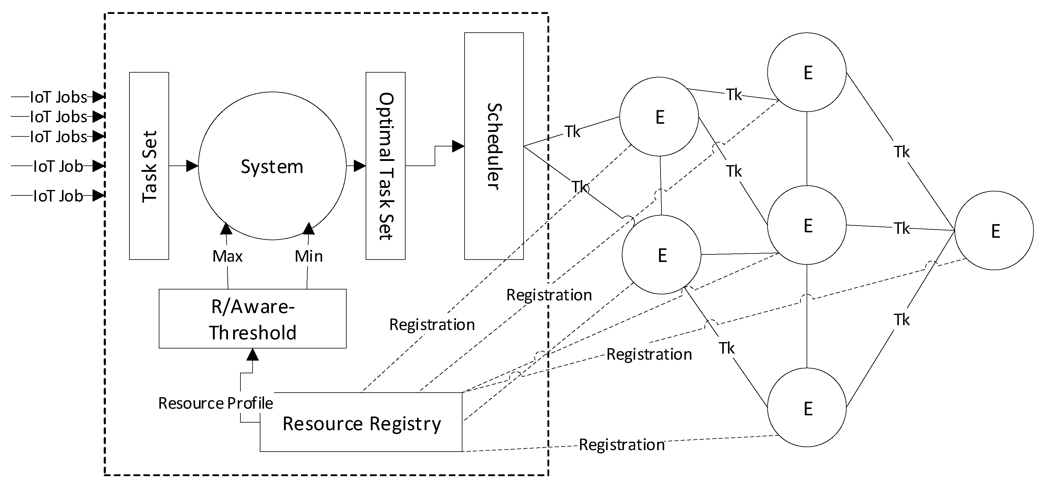
Figure 1 illustrates the black box representation of the proposed system model. The primary purpose is to take IoT task sets and resource profiles and tune them in such a way to produce optimal jobs that consume fewer clock cycles and hence less power. Inputs to the proposed system are resource profiles and task sets. The output is the optimal task sets which can be passed to the IoT scheduler. The scheduler schedules tasks on IoT edge-nodes.

The design of RT-IoT systems should be modelled in such a way that it must consume constrained resources wisely. Power and energy are among the constrained resources that play a vital role in the design of tasks and scheduling strategies. The average power P consumed by a microprocessor is given by Equation (1):

$$P=V_{cc}xI,$$

(1)

where $V_{cc}$ is the supply voltage and I is the average current. Similarly, the power is directly proportional to the energy consumption of an input task. Therefore, the average energy E is given by Equation (2):

$$E=PxT,$$

(2)

where P is the average power and T is the execution time of the input task. The execution time T is a function of clock cycles consumed by input program and is given by Equation (3):

$$T=N_{cc}x{C}_p,$$

(3)

where $N_{cc}$ is the number of clock cycles and $C_p$ is the period of clock cycles. Combining Equations (1)–(3) gives rise to Equation (5):

$$E=V_{cc}xIx{N}_{cc}x{C}_p,$$

(4)

if the remaining parameters are kept constant, and then power and energy are directly proportional to the number of clock cycles:

$$E\propto N_{cc}.$$

(5)

Therefore, in this paper, we design a strategy to control the clock-cycles of scheduling algorithms based on the careful design of input tasks.

The effectiveness of an algorithm contributes to how many clock cycles it consumes during its lifespan, and it is known as computational complexity. Many algorithms define static complexity, which can be determined a priori. In contrast, many algorithms’ complexities are subjected to the input they take and vary according to the input provided.

Scheduling algorithms like RM, DM and EDF compute the hyper-period of input tasks to know the number of times the CPU clock runs. Thus, the computational complexity becomes dependent on the input tasks’ period. In this paper, we assume a multi-core platform comprised of c cores with the only constraint of $c\ge 2$. The task set denoted by $\mathsf{\Gamma }=\{{\tau }_1,{\tau }_2,{\tau }_3\dots {\tau }_n\}$. Every task instance has been characterized by three parameters: worst-case execution time of task ${\tau }_i$ denoted by $wce{t}_i$, $P_i$ is the inter-arrival time i.e., period of any two consecutive instances of task ${\tau }_i$ and $p_i$ is the priority of ${\tau }_i$. Other crucial factors are worth considering regarding tasks that are CPU utilization, which is denoted by $u_i$ and process utilization which is denoted by U. These two factors find whether a given task set $\mathsf{\Gamma }$ is schedulable on a given CPU of c cores. The CPU utilization and process utilization can be found by Equations (6) and (7), respectively:

$$u_i=wce{t}_i/P_i,$$

(6)

$$U=\sum _{i=1}^n{u}_i.$$

(7)

Historically, many researchers have suggested various criteria for the schedulability test. For instance, in [43,44], it has been pointed out that tasks will be schedulable for an RM algorithm on m processors if the utilization $u_i$ of every individual task ${\tau }_i$ does not exceed $m/3m-2$ and the total utilization is at most $m^2/3m-1$. It is discussed in [45] that Liu and Layland (1973) proposed the conditions of basic schedulability for RM and EDF to be a function of CPU Utilization bound, which is found in Equation (7). A set of n periodic tasks is schedulable by the RM algorithm if

$$\sum _{i=1}^n{U}_i\le n(2^{1/n}-1).$$

(8)

For EDF, under the same assumption, the same set of n periodic tasks is schedulable if

$$\sum _{i=1}^n{U}_i\le 1.$$

(9)

The utilization bound of RM is dependent on the number of tasks, and, for an infinite number of tasks, the utilization bound can be found by Equation (10).

$$\underset{n\to \infty }{lim}n(2^{1/n}-1)=ln2\approx 0.69.$$

(10)

This schedulability test is of paramount importance given the critical nature of hard real-time systems. The fact is that, in hard real-time systems, there is no luxury of even a mundane chance of failure out of the entire span of execution time. The problem arises when the algorithm passes the schedulability test, but the embedded IoT objects do not have sufficient resources to execute tasks due to the requirement of higher clock cycles than devices can support. It is pointed out that the primary wellspring of the issue is the high value of hyper-period. The computational complexity is the function of hyper-period and is computed in Equation (11):

$$O(n)=H(nlog(k))\{\forall n,k\in N\},$$

(11)

where n is the number of input tasks, k is the task instance to be run in each period and H is the hyper-period. Each algorithm forms task instances according to their implementation so k could be changed from one algorithm to another. Moreover, the hyper-period H of set of n tasks $\mathsf{\Gamma }$ can be found by Equation (12):

$$H=LCM\left\{{\tau }_i\right|1\le i\le n\},$$

(12)

where LCM is the least common multiple of tasks’ period and ${\tau }_i$ is an individual task.

At times, for some input tasks, the hyper-period gets enormously high and so too the computational complexity of the algorithm. Since these algorithms are needed to be run on IoT devices which have constrained capabilities concerning power and computation, so this becomes more catastrophic if hyper-period increases above a certain threshold.

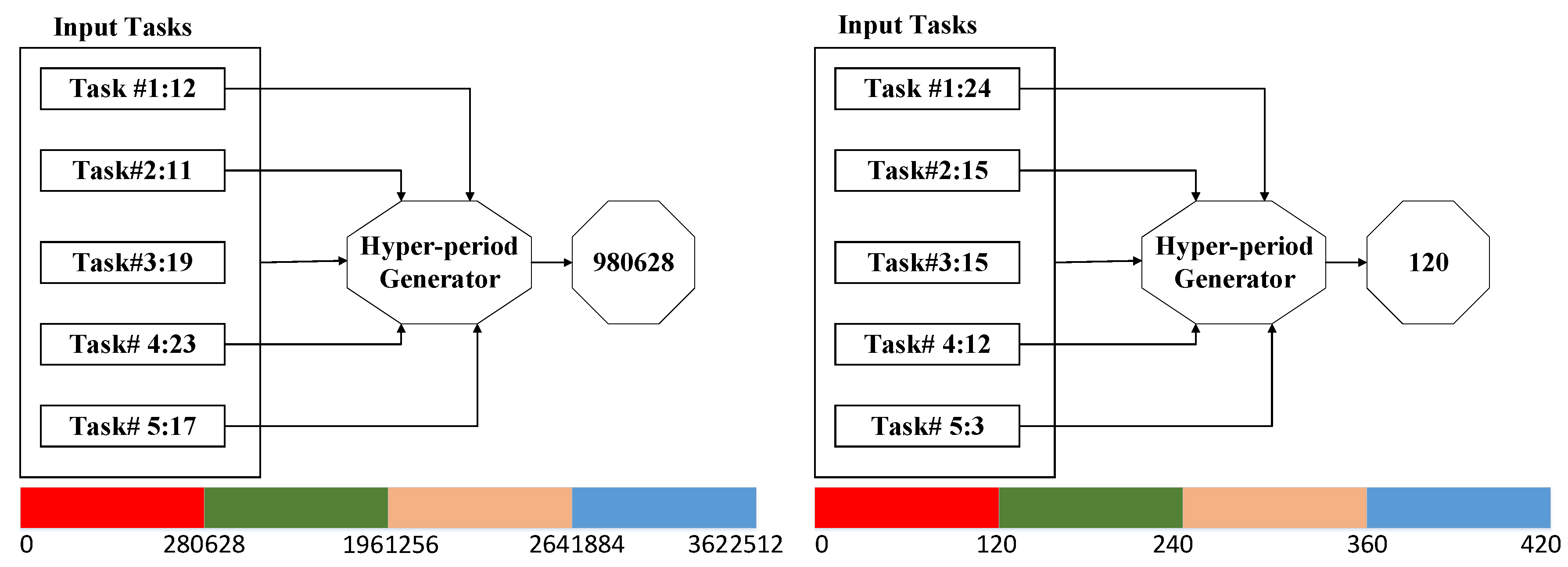
For instance, if a task set ${\mathsf{\Gamma }}_1=\{12,11,19,23,17\}$ is supplied as an input to Equation (12), the result produced of 980,628 is enormously high and no embedded device can have sufficient resources to fulfill the scheduling requirement of this task set. In contrast, if the same number of tasks with different periods as in ${\mathsf{\Gamma }}_2=\{24,15,15,12,3\}$ is given as an input to Equation (12), the result 120 is produced, which is well within the system available resource. This can be described in Figure 2.

The left part of Figure 2 shows that the task set has a high hyper-period and thus it consumes more CPU cycles. In contrast, the task set on the right side shows a considerably lower value of the hyper-period and thus consumes fewer clock cycles. The strip below each task set represents that, after the hyper-period amount of clock cycles, the same scheduling pattern will be repeated. It is formally called a period optimisation problem and the period is recognised as the optimisation parameter.

Let us assume that $J_i(P_i)$ is a monotonously increasing function of period $P_i$ when $P_i\ge 0$, the loss index (U) of the system is found by Equation (13):

$$U=\sum _{{\tau }_i\in \mathsf{\Gamma }}{w}_i{J}_i(P_i),$$

(13)

where $w_i$ is a constant defined by a user representing the priority of the ith task. For example, in a typical IoT context, if a readSensor task has $w_i=1$ and turnOnLED has $w_i=0.5$, it would mean that the former task is more important than the latter in terms of power-consumption.

Real-time scheduling and controlling modules in general real-time systems receive the constraints imposed on selecting the period of input tasks, and it is generated in a bounded interval $(P_i^{min},P_i^{max}$ according to these constraints. The constraints can be power-efficiency, response time and steady-state accuracy. One crucial constraint to consider is a multi-core utilization bound, which plays a significant role in guaranteeing schedulability. For the RM algorithm, total system utilization and individual task utilization need to be within the computed bound as in Equations (7)–(9).

On the basis of the above claims, the period optimisation problem is categorised as a nonlinear constraint optimiser as in Equation (14):

$$minJ=\sum _{{\tau }_i\in \mathsf{\Gamma }}{w}_i{J}_i(P_i),\left\{\begin{array}{c}wce{t}_i\le P_i\hfill \\ U\le U_{bound},\hfill \\ P_i^{min}\le P_i\le P_i^{max}.\hfill \end{array}\right.$$

(14)

4. Proposed Work

In an RT-IoT system, the fundamental motivation is to achieve the same accuracy of the jobs within defined timing constraints. An example use case of RT-IoT systems is a patient monitoring system installed in an emergency ward. If the monitoring system is not able to execute tasks on time, it could lead to severe conditions.

Table 1. Real-time tasks related to a Patient Monitoring System in an IoT-based SmartHealth Domain.

S.No	Task Name	Description	Type
T1	SampleInformation	The samples of physical status of the patients is taken	Periodic
T2	VerifyData	Verify sampled data for emergent pattern	Periodic
T3	AnalyzePulse	Analysis of Patients’ pulse	Periodic
T4	AnalyzeBloodPressure	Analysis of Patients’ blood pressure	Periodic
T6	AnalyzeCardio	Analysis of Patients’ cardiogram	Periodic
T7	IsEmergent	Based on the previous tasks, it finds whether the patient state is emergent or not	Periodic
T8	ProduceAlarm	Based on Emergent Situation, alarm is produced	Event-Driven

shows some of the IoT tasks along with their description and type in the example use case scenario.

In this paper, we present a systematic approach to control the admission of such periodic tasks to keep the hyper-period within a certain optimal threshold so that it can guarantee successful execution within their stringent timing constraints. The optimal threshold is selected based on the IoT devices’ profile and the number of resources connected to them. The detailed method of finding the optimal threshold will be described in the subsequent subsection. Moreover, the proposed approach allows tasks of any possible period value. The paper has two main parts: first is the selection of optimal threshold and second is the selection of task sets within the optimal threshold. Figure 3 shows the overall flowchart of the proposed approach. The tasks’ admission control unit computes the hyper-period of input tasks. The hyper-period is then compared with the optimal threshold. The optimal threshold is selected using Optimization Function and Constraints and using the profile of the connected physical IoT Device.

If the hyper-period falls within the threshold, it is then passed to a real-time scheduler. However, if the hyper-period does not fall within the threshold range, tasks are seeded back to admission control to tune periods of tasks and this process will go on until the desired hyper-period is achieved. The overhead of the algorithm, also called noise of the application, is the number of CPU cycles wasted in finding the optimal set of periods for input tasks. The overhead is incremented after each failed attempt, and the final value of the overhead represents total attempts it made for finding the optimal hyper-period. The threshold is also dynamically adjusted based on IoT resources and IoT devices. The mechanism for the dynamic threshold adjustment is described in the subsequent section. Once the hyper-period is fixed below the optimal threshold, tasks are passed to the Scheduler where any real-time scheduling algorithm is applied. As mentioned in the Introduction section, this method is generic and targets any class of algorithms. This is why the Scheduler can implement any algorithm depending on application context and requirements. In this paper, we use algo1 as RM and algo2 as EDF and is generic for any algorithm algo n. The approach used in this research is adaptive with respect to resource awareness. It is adaptive in a sense that the threshold is all the time adjusted and safe values can be assigned based on the IoT Device’s profile and IoT resources connected to it. For instance, in case a new IoT resource is registered to the IoT device, the system will re-compute the minimum and maximum threshold to cope with the added resource.

4.1. Optimal Threshold

In this section, a detailed approach for finding optimal threshold has been described. A threshold is a number which indicates that within available resources the task set can be executed and real-time requirements of tasks can be safely ensured. It is crucial as if this threshold is not carefully designed devices will run out of clock cycles and as a result, the CPU will not be able to schedule one or more tasks. In this paper, we introduce the concept of resource-aware threshold selection which will set the threshold according to IoT resources. The threshold can be adjusted in case a resource is registered or deleted from the IoT server. The system maintains the threshold in a bounded interval $[T{h}^{min},T{h}^{max}]$. $T{h}^{min}$ is the minimum threshold while $T{h}^{max}$ is the maximum value after which the system can not safely schedule tasks. The correct value of the threshold can be determined by investigating the profiles of embedded devices and available resources attached to them. For each device, semantic ontologies are maintained which help in dynamically finding attributes of the device that cater to the threshold and compute the threshold from the actual values of these attributes.

In recent times, a diverse number of IoT devices has been employed in RT-IoT applications each having distinguished characteristics. Some of the notable hardware include Raspberry Pi, Edison Development Board and Arduino. These are such powerful toolkits that they can be used as IoT gateways and servers. In contrast, some devices are fabricated for a dedicated purpose and have limited memory and other resources. These can only be used as edge-nodes in a typical IoT scenario [46].

Let’s assume D represents a set of IoT devices $\{D_1,D_2,\dots ,D_n\}$ that interconnects to make a mashup of heterogeneous IoT devices. For every device $D_i$, ontologies are maintained keeping the information about device type, device memory, flash memory and the number of resources connected to it. This information is stored and often referred to as Device Profile.

The threshold $T{h}_i$ of an individual device $D_i$ depends on the CPU speed $C_i$, Main Memory $M{M}_i$, Flash Memory $F{M}_i$ and The number of resources connected to it $R_i$.

Lemma 1.

Threshold $T{h}_i$ of an embedded device $D_i$ is directly proportional to the speed of CPU $C_i$, the memory it contains and the flash memory it has.

Lemma 2.

Threshold $T{h}_i$ of an embedded device $D_i$ is inversely proportional to the number of physical resources $R_i$ connected to it.

Lemma 3.

The minimum threshold $T{h}^{min}$ of the system is the value which can be satisfied using only flash memory.

Lemma 4.

The maximum threshold $T{h}^{max}$ of the system is the value which if increased can move the system into an unsafe state and thus the possibility of failing the deadline of one or more tasks does exist.

Based on the above lemmas, the minimum threshold and the maximum threshold can be determined using Equations (15) and (16):

$$T{h}_i^{min}=C_i\ast F{M}_i/R_i\left\{\begin{array}{c}\forall 1\le i\le n,\hfill \end{array}\right.$$

(15)

$$T{h}_i^{max}=C_i\ast M{M}_i/R_i\left\{\begin{array}{c}\forall 1\le i\le n.\hfill \end{array}\right.$$

(16)

The total minimum threshold for the system is defined by Equations (17) and (18):

$$T{h}^{min}=\sum _{i=1}^{n}T{h}_i^{min}\left\{\begin{array}{c}\forall 1\le i\le n,\hfill \end{array}\right.$$

(17)

$$T{h}^{max}=\sum _{i=1}^{n}T{h}_i^{max}\left\{\begin{array}{c}\forall 1\le i\le n.\hfill \end{array}\right.$$

(18)

$T{h}^{max}$ and $T{h}^{min}$ are seeded to Algorithms 1 and 2, and the threshold is adjusted based on the overhead of the algorithm. The overhead represents the mode of input tasks. In a scenario, when the algorithm’s overhead is high, it means that tasks are coming with high values of periods or the system is accepting more input tasks. In this situation, the threshold is dynamically adjusted to minimise the failure rate of tasks’ acceptance and decrease the rate of increase in overhead.

Algorithm 1 Adaptive Period Tuning Algorithm

1: $\mathit{ThresholdMin}\leftarrow \mathit{Based} \mathit{on} \mathit{Equation} (9)$ 2: $\mathit{ThresholdMax}\leftarrow \mathit{Based} \mathit{on} \mathit{Equation} (10)$ 3: $\mathit{InputTasks}\leftarrow \mathit{Set} \mathit{of} \mathit{initially} \mathit{admitted} \mathit{tasks} \mathit{Tn}$ 4: $\mathit{Hyper}-\mathit{period}\leftarrow \mathit{LCM}(\mathit{P}(\mathit{t}\mathit{1}), \mathit{P}(\mathit{t}\mathit{2}), \mathit{P}(\mathit{t}\mathit{3})..\mathit{P}(\mathit{tn}))$ 5: $\mathit{Overhead}\leftarrow 0$ 6: $\mathit{ThresholdCoefficient}\leftarrow 0$ 7: $\mathit{CurrentThreshold}\leftarrow \mathit{ThresholdMin}$ 8: loop: 9: while$True$do 10:     $\mathit{Hyper}-\mathit{period}\leftarrow 0$ 11:     $\mathit{periods}\leftarrow \left[\right]$ 12:     $\mathit{ThresholdCoefficient}\leftarrow \mathit{ThresholdCoefficient}+1$ 13:     $\mathit{Overhead}\leftarrow \mathit{Overhead}+1$ 14:     for all Tasks do 15:         $\mathit{period}(\mathit{i})\leftarrow \mathit{random}(\mathit{i})$ 16:         $\mathit{periods}\left[\right]\leftarrow \mathit{period}(\mathit{i})$ 17:     $\mathit{Hyper}-\mathit{period}\leftarrow \mathit{LCM}(\mathit{periods}[])$ 18:     if $\mathit{Hyper}-\mathit{period}>\mathit{CurrentThreshold}$ then 19:         $[\mathit{CuttentThreshold}, \mathit{ThresholdCoefficient}\leftarrow \mathit{FunctionCall}: \mathit{AdjustThreshold}(\mathit{CurrentThreshold}, \mathit{ThresholdCoefficient})$ 20:         $\mathit{Continue}$ 21:     else 22:         $\mathit{Hyper}-\mathit{period} \mathit{Tuning} \mathit{Done}$ 23:         $\mathit{break}$ 24: $\mathit{AlgorithmOverhead}\leftarrow \mathit{overhead}$ 25: $\mathit{OptimalThreshold}\leftarrow \mathit{CurrentThreshold}$

Algorithm 2 Resource-Aware Optimal Threshold Selection Algorithm

1: $\mathit{ThresholdMin}\leftarrow \mathit{Based} \mathit{on} \mathit{Equation} (9)$ 2: $\mathit{ThresholdMax}\leftarrow \mathit{Based} \mathit{on} \mathit{Equation} (10)$ 3: if$\mathit{ThresholdCoefficient}\ge 100$then 4:     $\mathit{ThresholdCoefficient}\leftarrow 0$ 5:     $\mathit{AdjustmentRate}\leftarrow (\mathit{ThresholdMax}-\mathit{CurrentThreshold})/\mathit{ThresholdMax}$ 6:     $\mathit{CurrentThreshold}\leftarrow \mathit{CurrentThreshold}+\mathit{CurrentThreshold}\ast \mathit{AdjustmentRate}$ 7:     if $\mathit{CurrentThreshold}\ge \mathit{ThresholdMax}$ then 8:         $\mathit{CurrentThreshold}\leftarrow \mathit{ThresholdMax}$ 9: return$\mathit{CurrentThreshold}, \mathit{ThresholdCoefficient}$

Algorithm 1 describes the overall approach to tune the hyper-period within the optimal threshold. The algorithm receives parameters like minimum threshold, maximum threshold, and set of input tasks. The overhead of the algorithm is initialised to 0. The hyper-period is computed and compared against the optimal threshold value. If it is less than the optimal threshold, the algorithm passes the optimal task set to the scheduler. In contrast, if it is higher than the optimal threshold, the overhead is incremented, and the process repeats until an optimal task set is achieved. The threshold is adjusted if the input tasks are coming with a high value of periods and there is more possibility of getting a higher value of threshold each time. The threshold adjustment has been performed in Algorithm 2. The algorithm is executed once after 100 times of failed attempts. The threshold is updated based on the current threshold and maximum threshold. The updated threshold is returned to Algorithm 1. Algorithm 1 now has more chance of accepting the tasks because it has adjusted the threshold based on the mode of input tasks. This adjustment goes on until it reaches the maximum threshold of the system. At this point, no more adjustment is performed, and the system is said to be saturated.

4.2. Complexity Analysis

In this section, the complexity analysis of the proposed algorithms is discussed. The prime motivation of this algorithm is to reduce the hyper-period of the real-time tasks which plays a pivotal role in the computational complexity of RM, EDF, and many other similar algorithms. For instance, the complexity of the RM algorithm is $O(nlogn),$ where n represents the hyper-period. The more the hyper-period, the higher the clock cycles it will consume and vice versa. Algorithm 1 has two loops. Thus, it has the complexity in the order of $O(n^2)$. The worst-case complexity of the system is when the if block executes every time, and the loop continues. In this case, the saturation will occur, and the total complexity will be the number of tasks times the overhead. The best-case is when the else block executes in the first iteration. In this case, the complexity will be equal to the number of tasks. Either way, the hyper-period produced as a result will significantly help in decreasing the overall clock cycles of the algorithm, and hence the complexity of the system will also be decreased, and this is the primary rationale behind this work.

5. Interaction Model

In this section of the paper, the interaction among various elements during the period selection is described. Figure 4 depicts the sequence of operations among different modules of the proposed work. The Task Admission Controller module initialises the task set with random values and parses the period from the task set which contains other attributes like worst-case execution time, arrival time and priority.

The Device Management module loads the profile of IoT devices which is attached to different IoT gateways. It is necessary for optimal threshold selection. The optimal threshold has a significant impact on the overhead of the algorithm and the overall computational complexity of the scheduling algorithm. When the profile is loaded, the Constraint Provider module loads constraints and using parameters the Optimal Parameter Analyzer module designs the optimal threshold based on the Optimization function, constraints and IoT devices’ profile. The optimal threshold is loaded to the Hyper-period Tuner module. Task Admission Controller also loads the period from the task set to the aforementioned unit. The Hyper-period Tuner continuously tunes the periods until it falls within the optimal threshold. Once the loop is finished, the overhead is passed to an Optimal Parameter Analyzer, and the task set is given to the IoT Scheduler. The IoT Scheduler applies any algorithm under study, and the result is provided back to the Device Management Controller. The Device Management Controller finally uses the scheduling result to schedule IoT tasks on different devices.

6. Implementation Setup

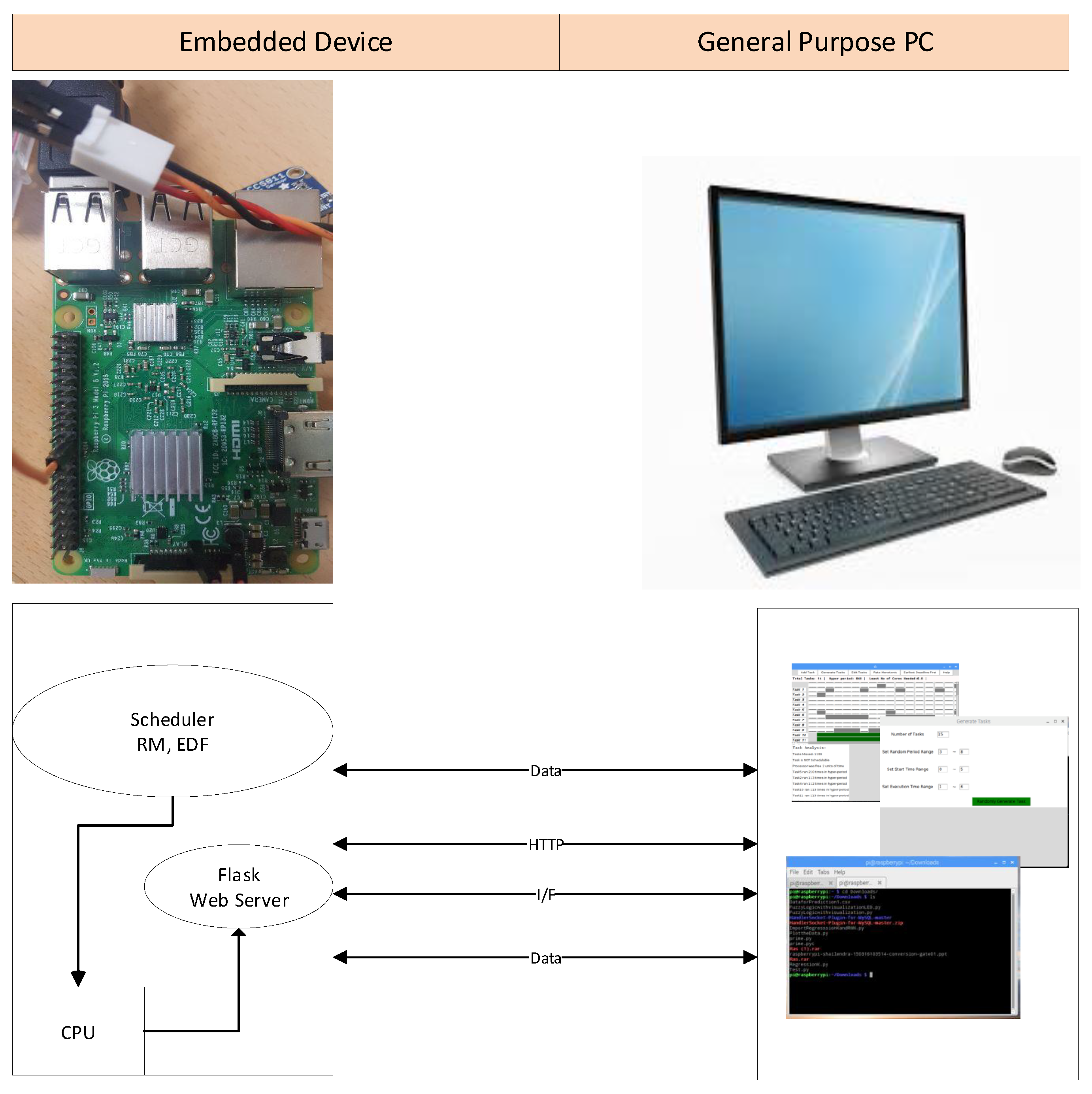
This section gives an overview of tools and technologies used in implementing and evaluating the proposed work. The development of this work is aimed to be run on general purpose machine and an embedded device as outlined in Figure 5.

This work utilizes some functional features of the web tool proposed in [47].

Table 2. Specification of implementation environment of general purpose PC.

System Parameter	Value
Operating System	Windows
CPU	Intel (R) Core(TM) i5-4570 CPU @ 3.20 GHz
Primary Memory	8 GB
Integrated Development Environment (IDE)	PyCharm, Sublime Text 3
Framework	Flask Micro Framework
Core Programming Language	Python
Libraries	Jinja 2, CSV Parser, Bootstrap 3, HTML 5/CSS3
Persistance	CSV

describes the technologies used on general purpose machine.

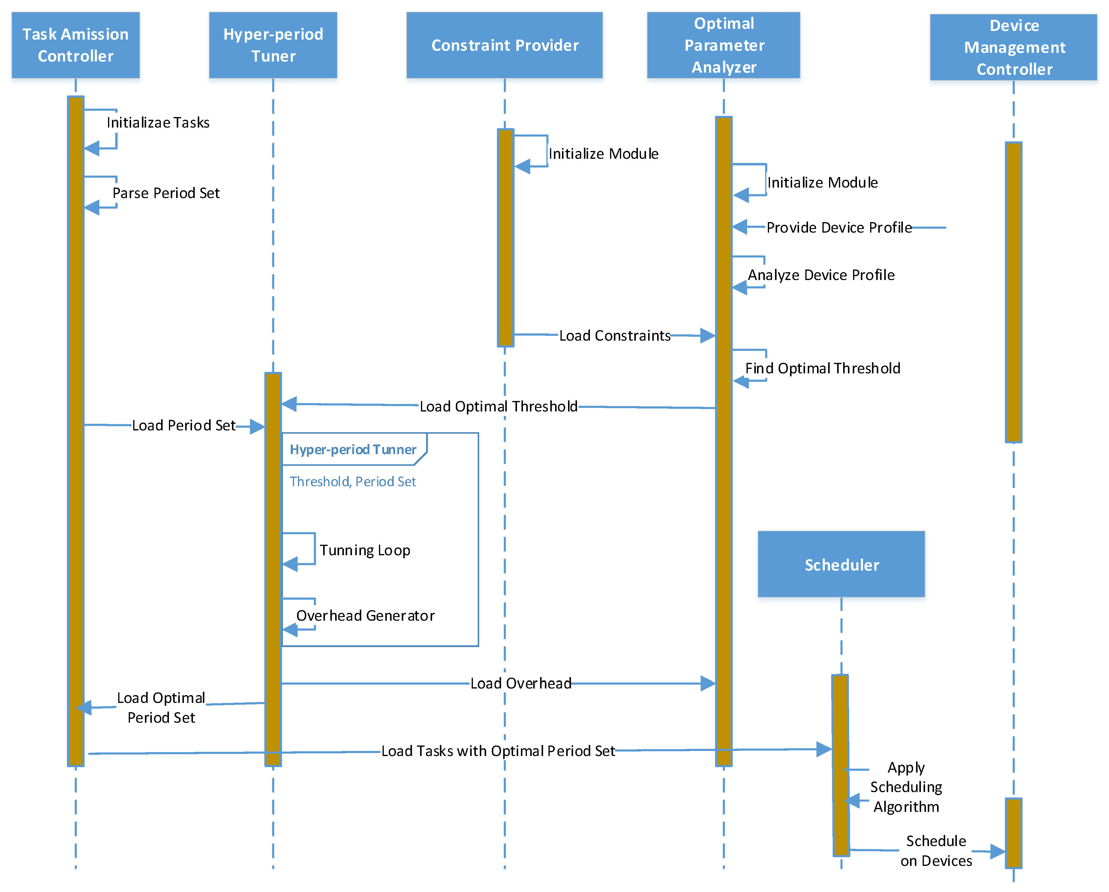
The scheduler communicates with a Raspberry Pi-based IoT server to which numerous physical resources are connected. In this paper, Raspberry Pi is used because it is relatively cheap and readily available everywhere. Development tools on a general purpose PC and the Raspberry Pi-based IoT server communicate using HTTP protocol and send a hyper-period and other information back and forth. Modules like Task Controller, Optimal Parameter Analyzer, and Constraint Provider are implemented on the PC end while the Scheduler and Device Management Controller are implemented on the Embedded Raspberry Pi end, which serves as a gateway for IoT physical objects. The specifications of the Raspberry Pi-based implementation environment are manifested in

Table 3. Specification of implementation environment of the Raspberry Pi embedded system.

System Parameter	Value
Hardware	Raspberry Pi 3 Model B
Operating System	Raspbian
Memory	1 GB
Server	Flask Webserver
Libraries	GPIO, CSVReader, Jinja Template, Bootstrap 3, HTML 5/CSS3
IDE	Vim, PyCharm (Remote Access)
Programming Language	Python 3

.

We use Python as a core programming language. Python is a general purpose popular programming language. It is widely used for developing web-based applications, desktop-based applications, data analysis and simulation. It has vast community and a strong developer’s bench. We used Python for three reasons. Firstly, it is equally popular among web programmers and a scientist. Secondly, it is effortless to learn and adapt and, finally, it has powerful API support. In this research, we used Python 3.5. Moreover, it is strongly recommended that following a design pattern for implementing the tool is always time-saving and leads to very organised and maintainable source code. This is why we use Flask; a Model View Controller (MVC) mini-framework [48]. It is mini-framework in a sense that it does not utilise the full-fledged features of an MVC framework. It uses only those modules which are required on demand thus brings efficiency in its core. Modules of the framework are loosely coupled and can be utilised as per demand. For Front-End technologies, we use HTML5, CSS3, and JavaScript. We also use Bootstrap 3 and a powerful Front-End framework for re-using the code and making the tool responsive to run on mobile screens too [49]. The significant part of the presentation has been developed with the help of a Jinja Templating Engine.

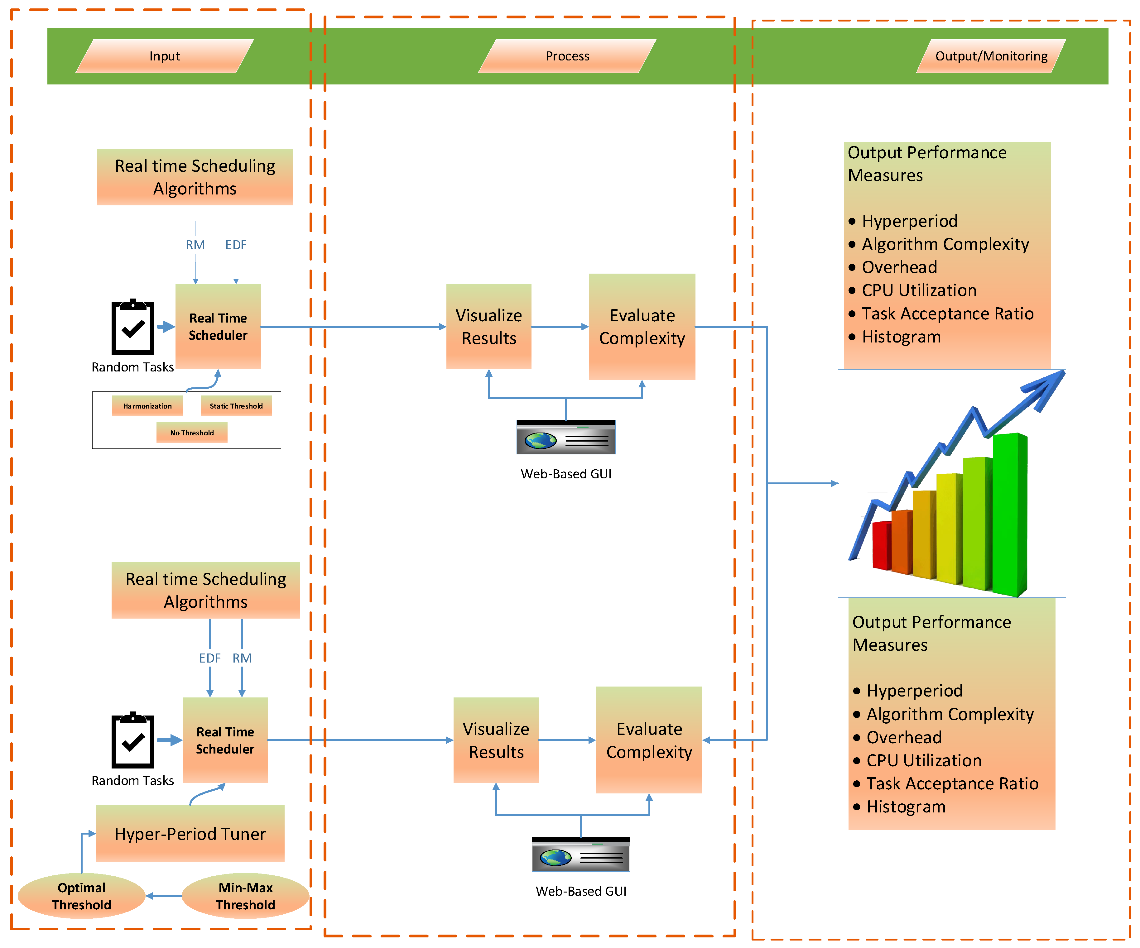
As part of the implementation of this work, a Web-based Graphical User Interface (GUI) based on [47] is utilised to simulate various algorithms and to compute the relative complexity of input tasks of both existing approaches and the proposed approach. The flow of different processes for experimental scenarios is portrayed in Figure 6. Input tasks are admitted for scheduling using existing approaches like static threshold, no threshold, and harmonization approach and then using the proposed optimal threshold approach.

Web-based GUI is used to aid in the visualisation of results. In the proposed approach, the optimal threshold is computed and passed to the hyper-period tuner. A hyper-period tuner generates an optimal task set based on a computed hyper-period and passes it to the real-time scheduler. The real-time scheduler schedules the tasks based on the supplied algorithm. In this work, we consider RM and EDF. The results from both the proposed approach and existing approaches are passed to the web-based application which visualises the result on better User eXperience (UX) interfaces. Complexities of all approaches are evaluated, and output measures of algorithms are highlighted with the help of graphs. Output measures include hyper-period, complexity, overhead, CPU utilization, task acceptance ratio, and period frequency.

7. Experimental Results

In order to highlight the contribution and significance of this work, numbers of experiments are carried out, and the results are recorded. The parameters of the real-time tasks can be any of the numbers of tasks, period range, arrival range, and execution time range. The performance of the proposed approach has been measured with different output measures as highlighted in Figure 6. We start with varying the number of input tasks and observing results and then changing the period range of these input tasks by making the rest of the task parameters constant and noting the result. Finally, the same experimentation has been performed by varying the arrival and execution time range. The effect of these parameters does not reflect on hyper-period but rather on the number of attempts the algorithm makes to tune periods. We call this Overhead of the proposed algorithm. In the following subsections, the results of each scenario have been presented.

7.1. Input Tasks Load

Any real-time scheduling algorithm and the underlying embedded hardware depend on the number of tasks they process. It is referred to as Input load of the system. In this section, the input load is varied, and its effect is recorded. The rest of the parameters are kept constant to find the impact of the proposed work on the input load. The experiments are repeatedly performed for the various number of tasks starting from 2 to until 100 tasks. It can be seen from

Table 4. Scenario: Varying number of input tasks.

Input Tasks	Period Range	Execution Time Range	Arrival Time Range
2	1–10	1–5	1–5
4	1–10	1–5	1–5
6	1–10	1–5	1–5
8	1–10	1–5	1–5
10	1–10	1–5	1–5
12	1–10	1–5	1–5
14	1–10	1–5	1–5
16	1–10	1–5	1–5
18	1–10	1–5	1–5
20	1–10	1–5	1–5
25	1–10	1–5	1–5
50	1–10	1–5	1–5
75	1–10	1–5	1–5
100	1–10	1–5	1–5

that the rest of the parameters are kept constant to observe the effect of input tasks better.

Figure 7 shows the effect of hyper-period, optimal threshold and overhead for a varying number of input tasks.

It can be observed from Figure 7a. Even though the number of tasks rises, the hyper-period always falls within the optimal threshold. The top line shows that the optimal threshold and the hyper-period have always fallen below the threshold. The optimal threshold is adjusted as the number of tasks increases and so too for the hyper-period. The overhead is very nominal for less number of tasks, but, when tasks grow, the overhead starts to get noticed. The pattern of hyper-period is randomly growing with an increasing number of tasks; however, it always falls within the optimal threshold. For instance, the hyper-period for 12 tasks is more than that of 14 tasks. Similarly, for 75 tasks, the hyper-period is lower than that for 50 tasks. In Figure 7b, the effect of the optimal threshold is shown. As the tasks increase, there is more probability that the hyper-period will get a higher value. Thus, it will increase the overhead more than the minimum threshold. The minimum threshold is initially set to 500 and increased after every 100th failed iteration. The amount of increase is computed based on Algorithm 2. Once the threshold is adjusted to better adapt to the input load, the probability that the hyper-period will fall below the new optimal threshold increases.

7.2. Period Range

In this part of the experimentation, the period range of input tasks is varied, and its effect is recorded with respect to the hyper-period, optimal threshold, and overhead. Experiments have been performed for different period ranges as summarised in

Table 5. Scenario: Varying period range.

Input Tasks	Period Range	Execution Time Range	Arrival Time Range
10	1–15	1–5	1–5
10	1–20	1–5	1–5
10	1–25	1–5	1–5
10	1–30	1–5	1–5
10	1–35	1–5	1–5
10	1–40	1–5	1–5
10	1–45	1–5	1–5
10	1–50	1–5	1–5
10	1–60	1–5	1–5
10	1–70	1–5	1–5
10	1–80	1–5	1–5
10	1–90	1–5	1–5
10	1–100	1–5	1–5

.

Figure 8 exhibits the effect of the varying period range on the hyper-period, optimal threshold, and overhead. In Figure 8a, much like in case of input load, although the period range rises, but the hyper-period always falls within the optimal threshold. It is because it has been fine-tuned after a number of attempts. The top line shows that the optimal threshold and the hyper-period have always fallen below the optimal threshold. The optimal threshold and overhead keep on increasing as the period range broadens. The reason for this is that, for a broad range of periods, there is more probability that higher period values will appear and, as a result, the hyper-period computed will not satisfy the optimal threshold. Consequently, the optimal threshold also increases and so does the overhead.

Figure 8b explains the effect of the optimal threshold on the period range. The graph structure is similar to input load in a sense that, as the period range increases, there is more probability that the hyper-period will get a higher value. It will cause a more frequent adjustment in the optimal threshold, and, as a result, the overhead will also rise. Overall, the effect of the input tasks and the period range is similar, but, in the case of the period range, the increase in hyper-period, overhead and optimal threshold is sharper. Therefore, the impact of the period on hyper-period is more than that of the number of tasks.

7.3. Execution and Arrival Time Range

If the input tasks’ load and the period range are kept constant and the execution time range and arrival time range vary, it is foreseen that it will not affect the overhead and hyper-period of the system. The reason for this is that the execution time and arrival time of the tasks have no role in calculating the hyper-period of the tasks but rather on the overall CPU utilization of the input tasks.

Table 6. Scenario: Changing execution time and arrival time range.

Input Tasks	Period Range	Execution Time Range	Arrival Time Range
10	1–10	1–15	1–15
10	1–10	1–20	1–20
10	1–10	1–25	1–25
10	1–10	1–30	1–30
10	1–10	1–35	1–35
10	1–10	1–40	1–40
10	1–10	1–45	1–45
10	1–10	1–50	1–50
10	1–10	1–60	1–60
10	1–10	1–70	1–70
10	1–10	1–80	1–80
10	1–10	1–90	1–90
10	1–10	1–100	1–100

reviews the scenarios used for varying the execution range, and the rest of the parameters are kept fixed. The number of tasks is fixed as 10, the period is selected from 1 to 10, and, for each experiment, the corresponding parameter is changed. For brevity, we represent this in the same table for execution time as well as for arrival time.

Figure 9a reveals the effect of hyper-period, optimal threshold, and overhead on varying range of execution time. Due to adjusting the hyper-period, it always falls below the threshold, but, in contrast, the overhead shows some irregular patterns, and thus no relation of overhead can be drawn with the execution time range.

Figure 9b depicts the behaviour of hyper-period, optimal threshold, and overhead with respect to the change in the range of arrival time. The random plots of overhead and hyper-period confirm that the arrival time of the tasks also has no relationship to the parameters mentioned above.

7.4. CPU Utilization Bound

As discussed in previous sections, the utilization bound is very crucial in assessing the feasibility analysis of the system. For most of the algorithms, utilization bound value greater than one would imply that some tasks might not get CPU cycles and will be dropped eventually. The RM algorithm schedules tasks by assigning fixed priorities, and this has been done offline. The priority of a task relies upon its deadline. The shorter the deadline will be, the higher the priority of that task will be. On the other hand, the priority of the EDF is computed dynamically but also relied upon the deadline. The sooner the deadline of a task will be, the higher the priority will be. The utilization bound for RM is 0.69 (Equation (10)), but for EDF it should be less than 1 (Equation (9)). Ideally, 0.69 utilization means that 30% of the CPU is idle which indicates under-utilization. The harmonization approach increases the utilization near to 100% for RM algorithm, and this is one major motivation behind this approach. In this part of experiments, RM and EDF algorithms are applied to four approaches; no threshold, static threshold, harmonization and optimal threshold and the utilization bound is measured. Figure 10a shows the behaviour of RM for the four approaches. The plots show that the utilization bound for smaller task sets, i.e., less than 20, falls within 0.69. That being said, all the approaches meet the schedulability requirements of input tasks. In this case, the proposed algorithm is superior in a sense that the range of period choices is broader as compared to other approaches. When the number of tasks increases, the utilization bound is also increased. The main reason for this is that tasks may have a high execution time as compared to the period and thus contributes to more CPU utilization. The static threshold approach and no threshold give rise to utilization bound more than 0.69, and thus some tasks are likely to miss the deadline. The proposed approach is better regarding utilization bound as compared to harmonization, but the harmonization can schedule tasks even if utilization bound near to 1 at the cost of discrete period values. For the two remaining approaches, when the number of tasks increases more than 50, the utilization bound starts to rise more sharply, and, for 100 tasks, it is more than one, which would mean that some tasks will not be scheduled. When no threshold is applied, even for just over 20 tasks, the utilization bound gives higher values. Thus, it means that, even for a small set of tasks, some tasks will be missed.

In Figure 10b, the effect of EDF using the same approaches is investigated. Since the utilization bound for EDF is more than the RM, for harmonization, the optimal threshold and static threshold approaches, the utilization bound is close to 1. When no threshold is applied, if the number of tasks increases beyond 15, the tasks will not be scheduled due to a higher utilization bound. The utilization bound for feasible schedulability in the case of EDF is higher than RM since the priorities are dynamically computed and are changed according to the execution of tasks. Nevertheless, the approach to find a utilization bound for EDF is the same as RM. Consequently, the curves in both graphs look similar. The bottom line which represents the proposed optimal threshold approach has a utilization bound close to 0.7. It, therefore, proves the claim that the proposed approach works well for any priority system. With this utilization, the input tasks can be scheduled on a static-priority system like RM and a dynamic-priority system like EDF. The static threshold and harmonization produce a utilization bound close to 1, and thus it means that these approaches can also be employed in normal scenarios. As it is discussed in many places, this paper addresses more dynamic context like IoT and Industry 4.0, the following two approaches take specific attributes that are needed in these contexts. Harmonization suffers from the scalability as this approach allows a period of only specific discrete values. On the other hand, the static approach does not have as such constraints, but it can produce a very high overhead at times, which results in increasing the memory footprints of the system drastically.

7.5. Tasks Acceptance Ratio

We simulated five tasks ten times with different period range and measured the percentage of the time tasks accepted. The same experiment has been performed and compared with existing approaches that we used in the case of utilization bound experiments. The result of the simulation has been shown in Figure 11. On average, the proposed approach accepts more tasks than all existing methods. With increasing tasks, the probability of acceptance drops, but the rate of decrease in the proposed approach is much less as compared to other approaches. For more than 25 tasks, all other approaches plummet towards zero, and the acceptance probability is very low. For a higher number of tasks, the “No-threshold” approach accepts a task after 1000 tasks, which is very minute and not an acceptable situation for most real-time systems. The optimal threshold approach allows more than 20% of the tasks even for a more broad range of 1 to 100 and thus indicates a significant gain over other similar approaches.

7.6. Periods’ Histogram

As discussed in the earlier sections, the primary rationale behind this work is that, in most techniques, the periods are limited to certain numbers and thus a period with some specific value can’t participate. It is not acceptable in the IoT context in general and Industry 4.0 specifically where almost all objects will be doing some critical manufacturing activities. Harmonization and related approaches accept task sets with period values in the harmonic series. That being said, tasks with period values not falling in the series will not be permitted. To prove that the proposed system accepts a task with every integer value of period, 10 tasks are generated 20 times. The period range is kept constant between 1 and 10. The histogram of the period for different approaches is presented in Figure 12. For harmonization, the histogram is not balanced. For instance, value 2 is repeated 75 times and value 7 does not appear even once. On the other hand, the optimal threshold and static threshold performs identical, but an optimal threshold outperforms a static threshold in terms of overhead.

7.7. Threshold

In this section of the paper, the overall behaviour of the proposed work has been discussed with varying the threshold of the system. It is envisioned that the threshold can be set in a such a way that it can safely satisfy the constrained requirement of embedded systems. If the threshold is set high, then the chance of getting a high value of a hyper-period will be higher. A higher value of hyper-period would increase the power consumption of the system to some extent, but the overhead of the algorithm will be considerably less. If the threshold is set as low, then the proposed algorithm will take more cycles to adjust the hyper-period below a certain threshold. In other words, a seemingly less threshold will give rise to more overhead, and a high threshold will give rise to more power consumption. That being said, there is a trade-off between both parameter and this approach serves well in selecting the optimal threshold. Figure 13 shows the effect of the threshold on the overhead of the algorithm.

The overhead of the algorithm is measured with varying the threshold value from 50 to 1000. Figure 13 shows that the overhead decreases as the threshold value increases and vice versa.

The performance of the algorithm, on the other hand, decreases with the increasing value of the threshold. In addition, at some point where the threshold value is very high, the performance of both the proposed and existing approaches will be the same.

In Figure 14, the algorithm is run for the threshold value 50 to 1000, and the performance is measured in milliseconds (ms). It is clear that the threshold value has a high impact on the performance gain of the system. The lower the threshold will be, the higher will be the performance of the system and thus the performance gain.

In the view of the experimental results above, it is proved that the optimal threshold value is of paramount importance because setting an unnecessarily higher value could decrease the overhead of the algorithm at the cost of performance, whereas setting a smaller value will lead to more performance gain but can lose more time in adjusting periods and thus could lead to more overhead.

7.8. Performance Measure on Raspberry Pi

In this section of the paper, the performance of the proposed work is measured by implementing RM and EDF algorithms on a Raspberry Pi-based IoT device with specifications outlined in Table 2. These algorithms are performed using the same approaches we considered throughout the paper. The response time of the algorithms is measured in ms. Figure 15a shows the results of the RM algorithm. Harmonization gives the best response time due to the low hyper-period, and this is expected because the Harmonization idea originally was coined to improve the performance of RM algorithm by minimising the hyper-period. However, the proposed optimal threshold is also reasonably good, and the performance is not degraded for an increasing number of tasks. A static threshold performs better for smaller task sets but when the task sets grow, the response time also rises, and this is due to the overhead of algorithms. Finally, the No Threshold approach works reasonably for smaller tasks, but, as the tasks set increases to more than 20, the response time rockets up and the system becomes unusable.

Similarly, in the case of EDF in Figure 15b, the graph looks identical with that of Figure 15a, but, in this case, the proposed optimal threshold performs better than the harmonization. The reason for this is that the harmonization approach is introduced initially to improve the RM algorithm. Thus, for the dynamic-priority system, it is as impressive as in the case of RM. The other two approaches perform precisely similar to that of RM, i.e., performs reasonably for lower task sets but becomes unusable for massive task sets.

As shown in Figure 15, the scheduling algorithms are run for an increasing number of tasks, and the performance comparison is carried out. The performance deteriorated in both systems with a growing number of tasks, but, in the proposed solution, the degradation is steady, and, in the existing works, it is degrading exponentially.

8. Conclusions and Future Directions

In this paper, we discussed a novel approach to deal with the challenge of power consumption issues arises due to the high value of hyper-period in real-time IoT systems. We proposed an adaptive strategy for finding the optimal threshold. The optimal threshold dynamically adjusts according to IoT resources and their profiles. The proposed algorithm uses the optimal threshold to find a task set with a hyper-period below this threshold. It allows tasks only to admit if it contributes to a lower value of the hyper-period than the optimal threshold. Other approaches like Harmonization and static threshold is very popular, but they are not scalable for a dynamic context of Real-time IoT in a sense that they are not catering for IoT resource profiles and, moreover, allow a specific set of period values. The significance of the proposed approach is highlighted with a series of experiments and comparisons with its counterparts in terms of acceptance ratio, overhead and response time and the results have indicated significant improvements regarding CPU clock cycles and thus the power consumption. Moreover, within the optimal threshold, the input tasks can have any natural number of period value that is considered to be crucial in the design of tasks for more dynamic and advance contexts like IoT and Industry 4.0. As a future work, it is worth considering applying the approach on more advanced scheduling algorithms designed explicitly for IoT systems in a realistic IoT environment and highlight the impact of any natural period value on the scalability of these IoT applications.

References

1. Da Xu, L. Enterprise systems: State-of-the-art and future trends. IEEE Trans. Ind. Inform. 2011, 7, 630–640. [Google Scholar]
2. Vermesan, O.; Friess, P.; Guillemin, P.; Gusmeroli, S.; Sundmaeker, H.; Bassi, A.; Jubert, I.S.; Mazura, M.; Harrison, M.; Eisenhauer, M.; et al. Internet of things strategic research roadmap. Internet Things Glob. Technol. Soc. Trends 2011, 1, 9–52. [Google Scholar]
3. Friess, P. Internet of Things-Global Technological and Societal Trends From Smart Environments and Spaces to Green ICT; River Publishers: Gistrup, Denmark, 2011. [Google Scholar]
4. Xia, F.; Yang, L.T.; Wang, L.; Vinel, A. Internet of things. Int. J. Commun. Syst. 2012, 25, 1101. [Google Scholar] [CrossRef]
5. Guo, B.; Zhang, D.; Wang, Z.; Yu, Z.; Zhou, X. Opportunistic IoT: Exploring the harmonious interaction between human and the internet of things. J. Netw. Comput. Appl. 2013, 36, 1531–1539. [Google Scholar] [CrossRef]
6. Leu, J.S.; Chen, C.F.; Hsu, K.C. Improving heterogeneous SOA-based IoT message stability by shortest processing time scheduling. IEEE Trans. Serv. Comput. 2014, 7, 575–585. [Google Scholar] [CrossRef]
7. Ding, Y.; Jin, Y.; Ren, L.; Hao, K. An intelligent self-organization scheme for the internet of things. IEEE Comput. Intell. Mag. 2013, 8, 41–53. [Google Scholar] [CrossRef]
8. Vlacheas, P.; Giaffreda, R.; Stavroulaki, V.; Kelaidonis, D.; Foteinos, V.; Poulios, G.; Demestichas, P.; Somov, A.; Biswas, A.R.; Moessner, K. Enabling smart cities through a cognitive management framework for the internet of things. IEEE Commun. Mag. 2013, 51, 102–111. [Google Scholar] [CrossRef]
9. Lazarescu, M.T. Design of a WSN platform for long-term environmental monitoring for IoT applications. IEEE J. Emerg. Sel. Top. Circuits Syst. 2013, 3, 45–54. [Google Scholar] [CrossRef]
10. Lima, D.F.; Amazonas, J.R. TCNet: Trellis Coded Network-Implementation of QoS-aware Routing Protocols in WSNs. IEEE Lat. Am. Trans. 2013, 11, 969–974. [Google Scholar]
11. Liu, M.; Li, Z.; Guo, X.; Dutkiewicz, E. Performance analysis and optimization of handoff algorithms in heterogeneous wireless networks. IEEE Trans. Mob. Comput. 2008, 7, 846–857. [Google Scholar]
12. Hodges, S.; Taylor, S.; Villar, N.; Scott, J.; Bial, D.; Fischer, P.T. Prototyping connected devices for the internet of things. Computer 2013, 46, 26–34. [Google Scholar] [CrossRef]
13. Wollschlaeger, M.; Sauter, T.; Jasperneite, J. The future of industrial communication: Automation networks in the era of the Internet of Things and Industry 4.0. IEEE Ind. Electron. Mag. 2017, 11, 17–27. [Google Scholar] [CrossRef]
14. Ramamritham, K.; Stankovic, J.A. Scheduling algorithms and operating systems support for real-time systems. Proc. IEEE 1994, 82, 55–67. [Google Scholar] [CrossRef] [Green Version]
15. Sprunt, B.; Sha, L.; Lehoczky, J. Aperiodic task scheduling for hard-real-time systems. Real-Time Syst. 1989, 1, 27–60. [Google Scholar] [CrossRef]
16. Lee, E.A. Cyber physical systems: Design challenges. In Proceedings of the 11th IEEE Symposium on Object Oriented Real-Time Distributed Computing (ISORC), Orlando, FL, USA, 5–7 May 2008; IEEE: Piscataway, NJ, USA, 2008; pp. 363–369. [Google Scholar]
17. Lehoczky, J.; Sha, L.; Ding, Y. The rate monotonic scheduling algorithm: Exact characterization and average case behavior. In Proceedings of the Real Time Systems Symposium, Santa Monica, CA, USA, 5–7 December 1989; IEEE: Piscataway, NJ, USA, 1989; pp. 166–171. [Google Scholar]
18. Lipari, G. Earliest Deadline First; Scuola Superiore Sant’Anna: Pisa, Italy, 2005. [Google Scholar]
19. Goossens, J.; Macq, C. Limitation of the hyper-period in real-time periodic task set generation. In Proceedings of the RTS Embedded System (RTS’01); Citeseer, The Pennsylvania State University: State College, PA, USA, 2001. [Google Scholar]
20. Nasri, M.; Fohler, G.; Kargahi, M. A framework to construct customized harmonic periods for real-time systems. In Proceedings of the 2014 26th Euromicro Conference on Real-Time Systems (ECRTS), Madrid, Spain, 8–11 July 2014; IEEE: Piscataway, NJ, USA, 2014; pp. 211–220. [Google Scholar]
21. Nasri, M.; Fohler, G. An efficient method for assigning harmonic periods to hard real-time tasks with period ranges. In Proceedings of the 2015 27th Euromicro Conference on Real-Time Systems (ECRTS), 8–10 July 2015; IEEE: Piscataway, NJ, USA, 2015; pp. 149–159. [Google Scholar]
22. Chen, C.Y.; Hasan, M.; Mohan, S. Securing Real-Time Internet-of-Things. arXiv 2017, arXiv:1705.08489. [Google Scholar]
23. Singh, J.; Hussain, O.; Chang, E.; Dillon, T. Event handling for distributed real-time cyber-physical systems. In Proceedings of the 2012 IEEE 15th International Symposium on Object/Component/Service-Oriented Real-Time Distributed Computing (ISORC), Guangdong, China, 11–13 April 2012; IEEE: Piscataway, NJ, USA, 2012; pp. 23–30. [Google Scholar]
24. Chen, B.; Butler-Purry, K.L.; Goulart, A.; Kundur, D. Implementing a real-time cyber-physical system test bed in RTDS and OPNET. In Proceedings of the North American Power Symposium (NAPS), Pullman, WA, USA, 7–9 Septemebr 2014; IEEE: Piscataway, NJ, USA, 2014; pp. 1–6. [Google Scholar]
25. Park, S.; Kim, J.H.; Fox, G. Effective real-time scheduling algorithm for cyber physical systems society. Future Gener. Comput. Syst. 2014, 32, 253–259. [Google Scholar] [CrossRef]
26. Kim, J.E.; Abdelzaher, T.; Sha, L.; Bar-Noy, A.; Hobbs, R. Sporadic decision-centric data scheduling with normally-off sensors. In Proceedings of the 2016 IEEE Real-Time Systems Symposium (RTSS), Porto, Portugal, 29 November–2 December 2016; IEEE: Piscataway, NJ, USA, 2016; pp. 135–145. [Google Scholar]
27. Butt, M.M.; Jorswieck, E.A.; Marchetti, N. Energy efficient scheduling for loss tolerant iot applications with uninformed transmitter. In Proceedings of the 2017 IEEE International Conference on Communications Workshops (ICC Workshops), Paris, France, 21–25 May 2017; IEEE: Piscataway, NJ, USA, 2017; pp. 546–551. [Google Scholar] [Green Version]
28. Tiwari, V.; Malik, S.; Wolfe, A. Power analysis of embedded software: A first step towards software power minimization. IEEE Trans. Very Large Scale Integr. Syst. 1994, 2, 437–445. [Google Scholar] [CrossRef]
29. Brocal, V.; Balbastre, P.; Ballester, R.; Ripoll, I. Task period selection to minimize hyperperiod. In Proceedings of the 2011 IEEE 16th Conference on Emerging Technologies & Factory Automation (ETFA), Toulouse, France, 5–9 September 2011; IEEE: Piscataway, NJ, USA, 2011; pp. 1–4. [Google Scholar]
30. Seto, D.; Lehoczky, J.P.; Sha, L.; Shin, K.G. On task schedulability in real-time control systems. In Proceedings of the 17th IEEE Real-Time Systems Symposium, Washington, DC, USA, 4–6 December 1996; IEEE: Piscataway, NJ, USA, 1996; pp. 13–21. [Google Scholar]
31. Seto, D.; Lehoczky, J.P.; Sha, L. Task period selection and schedulability in real-time systems. In Proceedings of the The 19th IEEE Real-Time Systems Symposium, Madrid, Spain, 4 December 1998; IEEE: Piscataway, NJ, USA, 1998; pp. 188–198. [Google Scholar]
32. Palopoli, L.; Pinello, C.; Bicchi, A.; Sangiovanni-Vincentelli, A. Maximizing the stability radius of a set of systems under real-time scheduling constraints. IEEE Trans. Autom. Control 2005, 50, 1790–1795. [Google Scholar] [CrossRef]
33. Wu, Y.; Buttazzo, G.; Bini, E.; Cervin, A. Parameter selection for real-time controllers in resource-constrained systems. IEEE Trans. Ind. Inform. 2010, 6, 610–620. [Google Scholar] [CrossRef]
34. Bini, E.; Di Natale, M. Optimal task rate selection in fixed priority systems. In Proceedings of the 26th IEEE International Real-Time Systems Symposium (RTSS 2005), Miami, FL, USA, 5–8 December 2005; IEEE: Piscataway, NJ, USA, 2005. [Google Scholar]
35. Du, C.; Tan, L.; Dong, Y. Period selection for integrated controller tasks in cyber-physical systems. Chin. J. Aeronaut. 2015, 28, 894–902. [Google Scholar] [CrossRef]
36. Cervin, A.; Velasco, M.; Martí, P.; Camacho, A. Optimal online sampling period assignment: Theory and experiments. IEEE Trans. Control Syst. Technol. 2011, 19, 902–910. [Google Scholar] [CrossRef]
37. Cha, H.J.; Jeong, W.H.; Kim, J.C. Control-scheduling codesign exploiting trade-off between task periods and deadlines. Mob. Inf. Syst. 2016, 2016. [Google Scholar] [CrossRef]
38. Han, C.C.; Tyan, H.Y. A better polynomial-time schedulability test for real-time fixed-priority scheduling algorithms. In Proceedings of the 18th IEEE Real-Time Systems Symposium, San Francisco, CA, USA, 2–5 December 1997; IEEE: Piscataway, NJ, USA, 1997; pp. 36–45. [Google Scholar]
39. Xu, J. A method for adjusting the periods of periodic processes to reduce the least common multiple of the period lengths in real-time embedded systems. In Proceedings of the 2010 IEEE/ASME International Conference on Mechatronics and Embedded Systems and Applications (MESA), Qingdao, China, 15–17 July 2010; IEEE: Piscataway, NJ, USA, 2010; pp. 288–294. [Google Scholar]
40. Ripoll, I.; Ballester-Ripoll, R. Period selection for minimal hyperperiod in periodic task systems. IEEE Trans. Comput. 2013, 62, 1813–1822. [Google Scholar] [CrossRef]
41. Jeffay, K. The Real-Time Producer/Consumer Paradigm: A paradigm for the construction of efficient, predictable real-time systems. In Proceedings of the 1993 ACM/SIGAPP Symposium on Applied Computing: States of the Art and Practice, Indianapolis, IN, USA, 14–16 February 1993; ACM: New York, NY, USA, 1993; pp. 796–804. [Google Scholar]
42. Gerber, R.; Hong, S.; Saksena, M. Guaranteeing real-time requirements with resource-based calibration of periodic processes. IEEE Trans. Softw. Eng. 1995, 21, 579–592. [Google Scholar] [CrossRef] [Green Version]
43. Andersson, B.; Baruah, S.; Jonsson, J. Static-priority scheduling on multiprocessors. In Proceedings of the 22nd IEEE Real-Time Systems Symposium, (RTSS 2001), London, UK, 3–6 December 2001; IEEE: Piscataway, NJ, USA, 2001; pp. 193–202. [Google Scholar]
44. Baruah, S.K.; Goossens, J. Rate-monotonic scheduling on uniform multiprocessors. IEEE Trans. Comput. 2003, 52, 966–970. [Google Scholar] [CrossRef]
45. Buttazzo, G.C. Rate monotonic vs. EDF: Judgment day. Real-Time Syst. 2005, 29, 5–26. [Google Scholar] [CrossRef]
46. Hardware Comparison. 2018. Available online: https://www.postscapes.com/internet-of-things-hardware (accessed on 10 July 2018).
47. Ahmad, S.; Hang, L.; Kim, D.H. Design and Implementation of Cloud-Centric Configuration Repository for DIY IoT Applications. Sensors 2018, 18, 474. [Google Scholar] [CrossRef] [PubMed]
48. Flask. Web Development One Drop at a Time. 2018. Available online: http://flask.pocoo.org/ (accessed on 15 March 2018).
49. Bootstrap. 2018. Available online: https://getbootstrap.com/ (accessed on 15 March 2018).
Figure 1. General System block representation of the proposed work.
Processes 06 00090 g001
Figure 2. Hyper-period comparison of different task sets and its effect on CPU clock cycles.
Processes 06 00090 g002
Figure 3. Working flow diagram of the Proposed Approach.
Processes 06 00090 g003
Figure 4. Interaction model among different modules.
Processes 06 00090 g004
Figure 5. Implementation architecture.
Processes 06 00090 g005
Figure 6. Flow of different processes in experimental setup.
Processes 06 00090 g006
Figure 7. Scenario 1: The effect of varying Number of Input Tasks, given Period = 1–10, Execution Time Range = 1–5, Arrival Time Range = 1–5. (a) effect of hyper-period, optimal threshold and overhead on number of tasks; (b) effect of optimal threshold on the number of tasks.
Processes 06 00090 g007
Figure 8. Scenario 2: The effect of varying Period Range, given No. of Tasks = 1–10, Execution Time Range = 1–5, Arrival Time Range = 1–5. (a) effect of hyper-period, optimal threshold and overhead on period range; (b) effect of optimal threshold on period range.
Processes 06 00090 g008
Figure 9. Scenario 3: The effect of varying Execution and Arrival Range, given No. of Tasks = 10, Period Range = 1–10. (a) execution time range; (b) arrival time range.
Processes 06 00090 g009
Figure 10. Effect of CPU Utilization Bound on varying input task load for RM and EDF algorithms, given Period = 1–10, Execution Time Range = 1–5, Arrival Time Range = 1–5. (a) effect of CPU Utilization Bound on RM algorithm—Existing Approaches vs. Proposed Approach; (b) effect of CPU Utilization Bound on EDF algorithm—Existing Approaches vs. Proposed Approach.
Processes 06 00090 g010
Figure 11. Tasks Acceptance Ratio using various A=approaches for an increasing number of tasks.
Processes 06 00090 g011
Figure 12. Histogram of different values of periods.
Processes 06 00090 g012
Figure 13. Overhead vs. Threshold.
Processes 06 00090 g013
Figure 14. Overhead vs. Performance.
Processes 06 00090 g014
Figure 15. Performance Comparison of RM and EDF algorithms on Raspberry Pi-based Embedded IoT Device using various approaches. (a) performance of RM algorithm—Existing Approaches vs. Proposed Approach; (b) performance of EDF algorithm—Existing Approaches vs. Proposed Approach.
Processes 06 00090 g015aProcesses 06 00090 g015b