Modeling and Optimal Design of Absorbent Enhanced Ammonia Synthesis

Abstract

Synthetic ammonia produced from fossil fuels is essential for agriculture. However, the emissions-intensive nature of the Haber–Bosch process, as well as a depleting supply of these fossil fuels have motivated the production of ammonia using renewable sources of energy. Small-scale, distributed processes may better enable the use of renewables, but also result in a loss of economies of scale, so the high capital cost of the Haber–Bosch process may inhibit this paradigm shift. A process that operates at lower pressure and uses absorption rather than condensation to remove ammonia from unreacted nitrogen and hydrogen has been proposed as an alternative. In this work, a dynamic model of this absorbent-enhanced process is proposed and implemented in gPROMS ModelBuilder. This dynamic model is used to determine optimal designs of this process that minimize the 20-year net present cost at small scales of 100 kg/h to 10,000 kg/h when powered by wind energy. The capital cost of this process scales with a 0.77 capacity exponent, and at production scales below 6075 kg/h, it is less expensive than the conventional Haber–Bosch process.

1. Introduction

Synthetic ammonia is an important commodity in present day society. In 2015, 160 million tonnes of ammonia were produced globally, the majority of which was used either directly or as a building block for nitrogen fertilizer, and the global demand for ammonia is expected to grow steadily at an annual rate of 1.5% [1]. However, the hydrogen required for ammonia production is conventionally obtained from fossil fuels such as natural gas or coal [2]. Furthermore, conventional ammonia production is energy intensive; in fact, ammonia synthesis for nitrogen-based fertilizers is responsible for 1% of global energy consumption [3]. A finite and depleting supply of fossil resources, as well as a desire for increased sustainability of fertilizer production have motivated the idea of producing ammonia using renewable energy. Additionally, ammonia has the potential as an energy-dense, carbon neutral liquid fuel, which, when made using renewables, could be used in various applications such as long-term energy storage or transportation to further reduce carbon intensity [4,5]. A proposed production pathway for renewable ammonia is to use electricity generated from renewable sources such as wind or solar to obtain hydrogen from electrolysis, nitrogen from air and to power the ammonia synthesis process itself. Small-scale, distributed production of ammonia better enables the use of this renewable energy. Pursuant to this notion of small-scale renewable-powered ammonia synthesis, a 65-kg/day (2.71 kg/h) wind-powered Haber–Bosch process has been constructed in Morris, MN [6].

The economics of renewable-powered ammonia synthesis using the Haber–Bosch process have also been investigated. In [7], wind-powered ammonia production for the purpose of fuel on remote islands was considered. Small-scale ammonia production was shown to be economically viable only if diesel costs more than $10/gallon. This result may be viable for isolated communities, but does not lend itself to more widespread adoption. In [8], the economic feasibility of a grid-connected, offshore wind-powered ammonia facility was examined, and the synthesis loop was found to account for over 20% of the ammonia system capital cost. An isolated (not grid-connected) ammonia energy storage system was proposed in [9], and it was determined that the ammonia synthesis loop accounted for up to 25% of the total system capital cost. Evidently, reducing the capital cost of ammonia synthesis would aid in improving the economics of these systems. Taking a more expansive view, optimal ammonia fertilizer supply chains for Iowa and Minnesota were determined [10]. In addition to purchasing from conventional producers, the option to install small-scale wind-powered Haber–Bosch processes was available, but the optimal supply chains only included renewable ammonia synthesis when a carbon tax was imposed. This result provides further support for efforts to reduce the capital cost of ammonia synthesis.

The main driver of the capital cost in the Haber–Bosch process is high pressure, which leads to expensive compressors, as well as high wall thickness requirements for piping and vessels. However, significantly reducing the pressure in the Haber–Bosch process is difficult because doing so reduces reactor single pass conversion and also requires even lower temperatures for condensation of ammonia from unreacted hydrogen and nitrogen, thus increasing refrigeration demand. An alternative approach is absorbent-enhanced ammonia synthesis in which a bed of supported alkali metal salt replaces the conventional condenser [11,12]. This absorbent allows for more complete ammonia separation as compared to condensation, and subsequently, high ammonia production rates can be achieved while operating at lower pressures [13]. Additionally, ammonia absorption can occur around 200 ${}^{\circ }$C, meaning that cooling water can be used, rather than refrigeration, which is required in the Haber–Bosch process.

The promise of this absorbent-enhanced process has motivated the present work. First, we develop a model of this process (which is dynamic because absorption is inherently transient). We then use the model for design optimization to determine process design and operating conditions that minimize its net present cost (NPC) under the condition that the process is powered using only stranded wind energy at multiple small scales. The rest of the paper is structured as follows. Section 2 provides a description of the absorbent-enhanced process. Section 3 outlines the dynamic model of this process. Section 4 provides the formulation of the optimal design problem. The results of the optimal design problem at scales of 100 kg/h, 500 kg/h, 1000 kg/h, 5000 kg/h and 10,000 kg/h are presented in Section 5. The implications of the optimal design results as they pertain to the economics of the Haber–Bosch process are discussed in Section 6.

2. Process Description

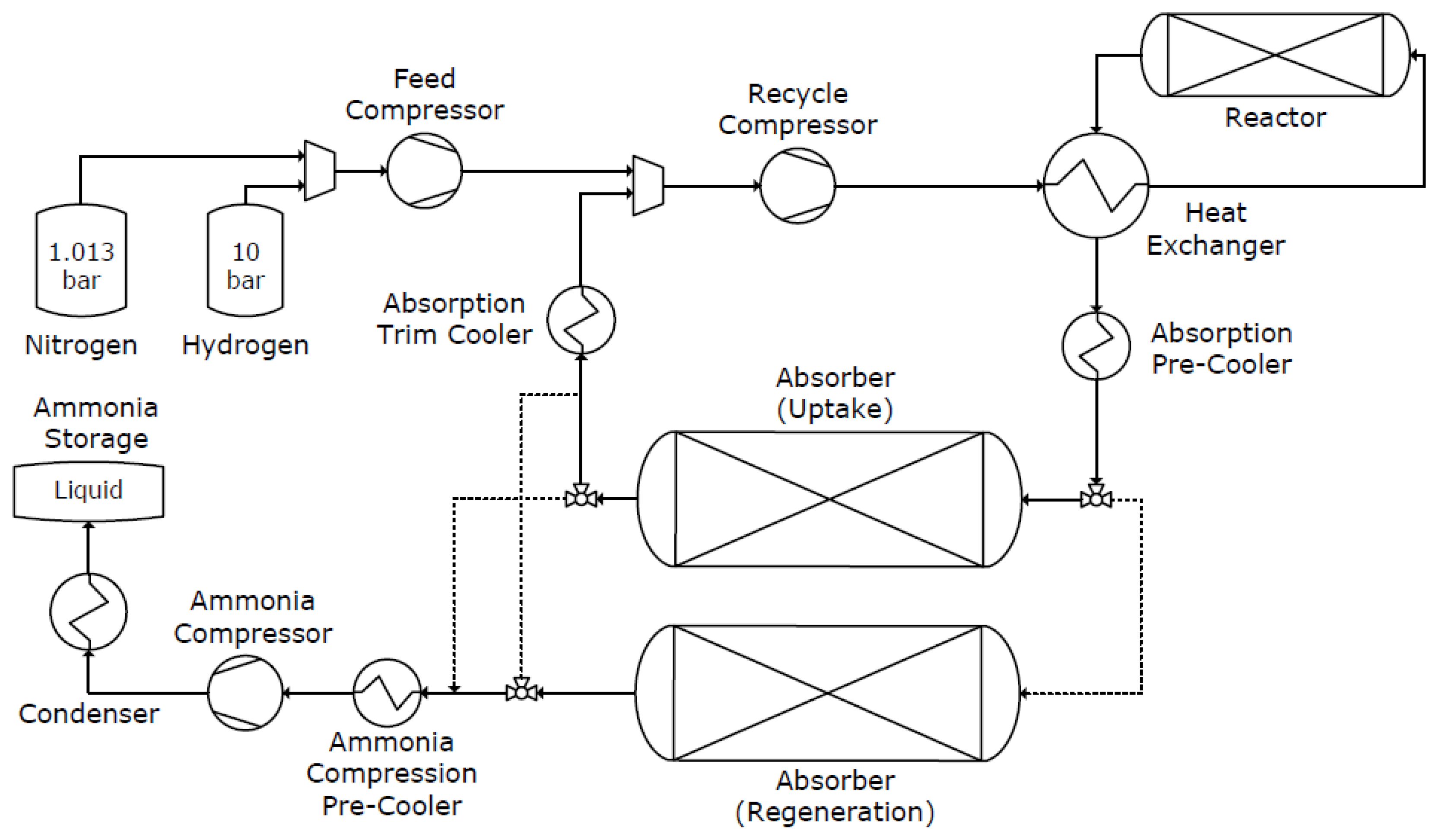
A flow diagram of the absorbent-enhanced ammonia synthesis process is given in Figure 1. Absorption is inherently transient, but the use of two beds allows for operation at a cyclic steady state. The process can naturally be partitioned into two distinct parts: reaction-absorption and desorption (regeneration). The feed to the reaction-absorption loop is a stoichiometric mixture of nitrogen at 1.013 bar (atmospheric pressure) and hydrogen at 10 bar (the outlet pressures of pressure-swing adsorption and electrolysis, respectively). These gases are compressed to the process operating pressure, which is between 15 and 30 bar (one order of magnitude lower than industrial conditions in the Haber–Bosch process), before being sent to a heat exchanger, which uses the reactor effluent to heat the feed gas to reaction temperature, which is around 400 ${}^{\circ }$C. The nitrogen and hydrogen then react over a fixed bed of wustite-based iron catalyst, which is the industrial standard, to form ammonia. The reactor effluent is partially cooled using the previously-mentioned heat exchanger and further cooled with cooling water to the absorption temperature, which is in the range of 100–200 ${}^{\circ }$C. The absorber is a fixed bed of magnesium chloride supported on silica [12], which serves to remove ammonia selectively through its absorption into the solid. The absorber effluent, which is primarily nitrogen and hydrogen with some unabsorbed ammonia, is then cooled to ensure safe operation of the recycle compressor, for its discharge temperature cannot exceed 150 ${}^{\circ }$C. These gases are mixed with the fresh feed.

At the end of an absorption cycle, once the absorber is deemed to be saturated, it is regenerated through a combination of heating to between 400 and 500 ${}^{\circ }$C and decreasing pressure by opening one end of the bed. This causes a reduction in the ammonia storage capacity of the absorbent, and subsequently, ammonia is released to the gas phase. This gas leaves the bed through the open end due to the imposed pressure gradient. The absorber effluent is cooled (to not damage the subsequent compressor), compressed and condensed so that it can be stored as a liquid. The release of ammonia occurs until the absorbent has been emptied and the bed pressure is equal to the pressure outside the vessel. Once this occurs, one bed volume of stoichiometric nitrogen and hydrogen is fed to the bed to displace the gaseous ammonia. The emptied bed is re-pressurized to the reaction-absorption pressure with a stoichiometric mixture of nitrogen and hydrogen and then reconnected to the reaction-absorption loop.

3. Mathematical Model

A dynamic model of the absorbent-enhanced process was created using gPROMS ModelBuilder 5.1 [14]. The individual unit models are described in this section, though they are largely standard to the PML Library in gPROMS. Physical properties such as mass-specific enthalpy $\widehat{H}$, density $\rho$ and viscosity $\mathsf{\mu }$ are calculated in Multiflash 6.1 [15] using temperature T, pressure P and mass composition $w_i$ as inputs. These calculations are based on the Redlich–Kwong–Soave equation of state for thermodynamic properties and the SuperTRAPP model [16] for transport properties.

3.1. Reactor

The ammonia synthesis reactor is modeled as an adiabatic pseudo-homogeneous plug flow reactor, with spatial variation in the axial direction z. Reactor specifications, which are taken as constant in the model, are given in

Table 1. Ammonia synthesis reactor specifications.

Parameter	Symbol	Specification
Bed Void Fraction ${}^1$	${\epsilon }_{bed}$	0.4
Catalyst Density, kg/m${}^3$	${\rho }_{cat}$	3000
Catalyst Particle Diameter, m	$d_p$	2 × 10${}^{-3}$

The bed void fraction is determined from the experimental setup in [13].

. The mass balance for species “i” is:

$${\epsilon }_{bed}\frac{\partial {\tilde{m}}_i}{\partial t}=-\frac{-1}{A_t}\frac{\partial {\dot{m}}_i}{\partial z}+{\nu }_{i}M{W}_i(1-{\epsilon }_{bed})r_{N{H}_3}$$

(1)

where ${\tilde{m}}_i$ is the species mass concentration in kg/m${}^3$, ${\dot{m}}_i$ is the species mass flow rate in kg/s, $r_{NH3}$ is the rate of ammonia formation in mol/(m${}_{cat}^3$ s), ${\nu }_i$ is the species stoichiometric coefficient, $M{W}_i$ is the species molecular weight in kg/mol, ${\epsilon }_{bed}$ is the bed void fraction and $A_t$ is the reactor tube cross-sectional area in m${}^2$. Writing the species balance in terms of mass, rather than moles, as is often the case, aids with the numerical solution in gPROMS. The energy balance is:

$$\frac{\partial \tilde{U}}{\partial t}=-\frac{-1}{A_t}\frac{\partial (\dot{m}\widehat{H})}{\partial z}+(-\Delta H_{rxn})(1-{\epsilon }_{bed})r_{N{H}_3}$$

(2)

where $\tilde{U}$ is the volume-specific internal energy in kJ/m${}^3$, $\dot{m}$ is the total mass flow rate in kg/s, $\widehat{H}$ is the mass specific enthalpy in kJ/kg and $\Delta H_{rxn}$ is the enthalpy of the ammonia synthesis reaction in kJ/mol. The volume specific internal energy is given by:

$$\tilde{U}=\rho \widehat{H}-P$$

(3)

where $\rho$ is the gas density in kg/m${}^3$ and P is pressure in bar. The pressure drop through the bed is given by the Ergun equation:

$$-\frac{\partial P}{\partial z}=v_s\left[\frac{150{(1-{\epsilon }_{bed})}^2}{{\epsilon }_{bed}^3{d}_p^2}\mu +\frac{1.75(1-{\epsilon }_{bed})}{{\epsilon }_{bed}^3{d}_p}\rho v_s\right]$$

(4)

where $v_s$ is the superficial velocity in m/s, $d_p$ is the particle diameter in m and $\mathsf{\mu }$ is the gas viscosity in kg/(m s). In the considered range of reactor operating conditions, the reactor particle Reynolds number is in the transitional region.

The rate of ammonia formation is given by the expression proposed in [17]:

$$r_{N{H}_3}=\frac{k(p_{N_2}{K}_a^2-p_{N{H}_3}^2/p_{H_2}^3)}{{(1+K_{N{H}_3}{p}_{N{H}_3}/p_{H_2}^{\omega })}^{2\alpha }}$$

(5)

where $p_i$ is the partial pressure of species “i” in atm and $\omega$ and $\alpha$ are fixed constants, the values of which are given in

Table 2. Ammonia synthesis reaction rate expression parameters.

Parameter	Value
$k_o$, mol/(m${}_{cat}^3$ s atm)	1.096 × 10${}^{10}$
$E_A$, J/mol	46,737
$K_{N{H}_{3}o}$, atm${}^{(1-\omega )}$	2.94 × 10${}^{-4}$
$E_{N{H}_3}$, J/mol	100,628
$\omega$	1.564
$\alpha$	0.64
$K_{a1}$	−2.691122
$K_{a2}$, 1/K	−5.519265 × 10${}^{-5}$
$K_{a3}$, 1/K${}^2$	1.848863 × 10${}^{-7}$
$K_{a4}$, K	2001.6
$K_{a5}$	2.6899

. The rate constant k, ammonia adsorption constant $K_{NH3}$ and equilibrium constant $K_a$ are given by:

$$k=k_{o}exp(-E_A/RT)$$

(6)

$$K_{N{H}_3}=K_{N{H}_{3}o}exp(E_{N{H}_3}/RT)$$

(7)

$${log}_{10}(K_a)={log}_{10}(K_{a1})+K_{a2}T+K_{a3}{T}^2+K_{a4}/T+K_{a5}$$

(8)

where T is the temperature in the bed in K, and values for all constants appearing in these expressions, such as $E_A$, are given in Table 2. This rate expression was chosen because it is non-infinite for zero ammonia partial pressure. This is not a concern when modeling the Haber–Bosch process because condensation never results in complete removal of ammonia from unreacted gases, but the condition of low ammonia partial pressure in the reactor inlet could potentially be achieved by the absorbent used in this process. It is noted that this kinetic expression is assumed to be valid for the lower total pressures investigated in this work and has not been validated experimentally at those conditions.

Low ammonia partial pressures also cause internal diffusion limitations in the ammonia synthesis catalyst [18]. Rigorously, this limitation would be accounted for by considering a heterogeneous reactor model with the simultaneous solution of fluid and particle phase mass balances. In order to reduce the computational complexity of the model while still accounting for mass transfer limitations, we generated an empirical expression for the ammonia partial pressure dependence of the catalyst effectiveness factor $\left(\eta \right)$:

$$\eta (p_{N{H}_3})=\frac{a_2{p}_{N{H}_3}^2+a_1{p}_{N{H}_3}+a_o}{b_2{p}_{N{H}_3}^2+b_1{p}_{N{H}_3}+1}$$

(9)

where values for the fitted constants are given in

Table 3. Ammonia reaction effectiveness factor parameters.

Parameter	${\mathit{a}}_{\mathit{o}}$	${\mathit{a}}_1$	${\mathit{a}}_2$	${\mathit{b}}_1$	${\mathit{b}}_2$
Value	0.03582	8.366	35.94	7.705	36.11

. This expression was obtained following the approach described in [19]. Effectiveness factor data were generated by the repeated “offline” solution of the particle mass balance for varying ammonia partial pressures. The empirical expression above was subsequently fit to the data.

3.2. Absorber

The model for the bulk fluid phase of the absorber considers axial dispersion and convection of mass and energy (the axial coordinate is z). The specifications, which are taken as constant in the absorber model, are given in

Table 4. Absorber specifications.

Parameter	Symbol	Specification
Bed Void Fraction ${}^1$	${\epsilon }_{bed}$	0.32
Absorbent Void Fraction ${}^1$	${\epsilon }_{abs}$	0.60
Total Void Fraction ${}^1$	${\epsilon }_{total}$	0.728
Absorbent Density, kg/m${}^3$	${\rho }_{cat}$	2507
Absorbent Particle Diameter, m	$d_p$	2 × 10${}^{-4}$
Absorbent Heat Capacity ${}^2$, kJ/(kg${}_{abs}$ K)	${\widehat{c}}_{p,abs}$	1.21

${}^1$ The bed and absorbent void fractions are determined from the experimental setup in [23]. ${}^2$ The absorbent heat capacity is assumed to be constant and is from [24].

. The mass balance for species “i” in an absorber tube is:

$${\epsilon }_{total}\frac{\partial {\tilde{m}}_i}{\partial t}=-\frac{-1}{A_t}\frac{\partial {\dot{m}}_i}{\partial z}+{\epsilon }_{bed}{D}_i\frac{{\partial }^2{\tilde{m}}_i}{\partial z^2}+M{W}_i(1-{\epsilon }_{total}){\rho }_{abs}(r_{des,i}-r_{abs,i})$$

(10)

where $D_i$ is the species effective dispersion coefficient in m${}^2$/s, which is calculated using the Wakao correlation for gas phase dispersion in packed beds [20], $r_{des,i}$ and $r_{abs,i}$ are species desorption and absorption rates in mol/(kg${}_{abs}$ s), ${\epsilon }_{total}$ is the total void fraction (accounting for the bed void fraction and absorbent particle porosity), ${\rho }_{abs}$ is the absorbent density in kg/m${}^3$ and $A_t$ is the absorber tube cross-sectional area in m${}^2$. It is noted that for the range of conditions in which absorption operates, the magnitude of dispersion coefficients is quite low such that dispersion could be neglected if desired. The absorber is non-adiabatic to accommodate the temperature difference required between absorption and desorption modes. The energy balance for an absorber tube is:

$$\frac{\partial \tilde{U}}{\partial t}=-\frac{-1}{A_t}\frac{\partial (\dot{m}\widehat{H})}{\partial z}+{\epsilon }_{bed}{\lambda }_{bed}\frac{{\partial }^{2}T}{\partial z^2}+\sum _{i=1}^{N_s}\Delta H_{abs}(1-{\epsilon }_{total}){\rho }_{abs}(r_{des,i}-r_{abs,i})+\frac{4q_{ext}}{d_T}$$

(11)

where T is the temperature of the fluid and absorbent in K (assumed to be identical), ${\lambda }_{bed}$ is the bed effective thermal conductivity in kW/(m K), which is calculated using the Specchia correlation [21], $\Delta H_{abs}$ is the enthalpy of absorption of species “i” in kJ/mol, $q_{ext}$ is the external heat addition or removal in kW and $d_T$ is the absorber tube diameter in m. The volumetric internal energy holdup is given by:

$$\tilde{U}={\epsilon }_{total}(\rho \widehat{H}-P)+(1-{\epsilon }_{total}){\rho }_{abs}{\widehat{c}}_{p,abs}T$$

(12)

where ${\widehat{c}}_{p,abs}$ is the absorbent heat capacity in kJ/(kg${}_{abs}$ K), the value of which is given in Table 4. Under this definition of volume-specific internal energy, sufficiently fast heat transfer between the solid and fluid phases is considered, such that their temperatures can be assumed to be identical [22]. As with the reactor, the pressure drop through the bed is given by the Ergun equation (Equation (4)), and the particle Reynolds number is again in the transitional region.

The solid phase (the absorbent) is volume-averaged; its mass balance has no explicit spatial dependence:

$$\frac{d{q}_i}{dt}=r_{abs,i}-r_{des,i}$$

(13)

where $q_i$ is the absorbed concentration of species “i” in mol/kg${}_{abs}$. The absorbent used in this system is selective to ammonia, and thus, the rates of absorption (and desorption) for hydrogen and nitrogen are zero. The rates of ammonia absorption and desorption were determined using data in [23]. The rate of ammonia absorption is given by:

$$r_{abs}=\left\{\begin{array}{cc}\frac{k_{abs}{[p_{N{H}_3}-p_{eq}\left(T\right)]}^7}{K_{abs}+{[p_{N{H}_3}-p_{eq}\left(T\right)]}^6},\hfill & \mathrm{for}{p}_{N{H}_3}>p_{eq},q_{N{H}_3}<q_{N{H}_3}^{max}\hfill \\ 0,\hfill & \mathrm{for}{p}_{N{H}_3}<p_{eq},q_{N{H}_3}=q_{N{H}_3}^{max}\hfill \end{array}\right.$$

(14)

It is noted that the exponents of 7 and 6 in the numerator and denominator, respectively, are chosen for fitting purposes, but are generally representative of a higher order (non-linear) rate. The rate of ammonia desorption is given by:

$$r_{des}=\left\{\begin{array}{cc}{k}_{des}[p_{eq}\left(T\right)-p_{N{H}_3}],\hfill & \mathrm{for}{p}_{N{H}_3}<p_{eq},q_{N{H}_3}>0\hfill \\ 0,\hfill & \mathrm{for}{p}_{N{H}_3}<p_{eq},q_{N{H}_3}=0\hfill \end{array}\right.$$

(15)

where $p_{N{H}_3}$ is ammonia partial pressure in bar, $q_{N{H}_3}^{max}$ is the maximum capacity of the absorbent based on stoichiometry in mol/kg${}_{abs}$ and $p_{eq}\left(T\right)$ is the absorbent equilibrium pressure, in bar, at a given temperature T. Values for constants $k_{abs}$, $K_{abs}$ and $k_{des}$ are given in

Table 5. Ammonia absorption and desorption rate parameters.

Parameter	Value
$k_a$, mol${}_N{H}_3$/(kg${}_{abs}$ bar s)	0.4668
K, bar${}^6$	5 × 10${}^{-24}$
$k_d$, mol${}_N{H}_3$/(kg${}_{abs}$ bar s)	7.002 × 10${}^{-3}$

. For this work, the maximum stoichiometric capacity of the MgCl${}_2$ absorbent is assumed (conservatively) to be that given by a 1:1 molar ratio of ammonia to salt, which corresponds to a maximum absorbed concentration of 10.5 mol${}_{N{H}_3}$/kg${}_{MgC{l}_2}$. Given that the solid phase contains only 40% salt by weight, the effective maximum absorbed concentration is 4.2 mol${}_{N{H}_3}$/kg${}_{abs}$.

The temperature dependence of the equilibrium pressure is given by:

$$ln(\frac{p_{crit}\left(T\right)}{p_{crit,ref}})=-\frac{\Delta H_{abs}}{R}\left(\frac{1}{T}-\frac{1}{T_{ref}}\right)$$

(16)

where the reference equilibrium pressure-temperature pair ($p_{crit,ref}$ and $T_{ref}$) and the heat of absorption $\Delta H_{abs}$ are from [25] and are given in

Table 6. Absorbent equilibrium pressure temperature dependence parameters.

Parameter	Value
$p_{crit,ref}$, bar	1
$\Delta H_{abs}$, J/mol	−87,000
$T_{ref}$, K	648.05

.

3.3. Compressor

Compression is assumed to by polytropic, so the compressor outlet temperature $T_{out}$ and power requirement ${\dot{W}}_{comp}$ are given by the following equations:

$$T_{out}=T_{in}{(\frac{P_{out}}{P_{in}})}^{\frac{n-1}{n}}$$

(17)

$${\dot{W}}_{comp}=\dot{m}\frac{n}{(n-1){\eta }_{poly}{\eta }_{elec}}\frac{z_{in}R{T}_{in}}{M{W}_{gas}}\left[{(\frac{P_{out}}{P_{in}})}^{\frac{n-1}{n}}-1\right]$$

(18)

where $T_{in}$ is the inlet temperature in K, $P_{in}$ and $P_{out}$ are the inlet and outlet pressures in bar, $\dot{m}$ is the mass flow rate in kg/s and $z_{in}$ is the compressibility factor at inlet conditions. The values of polytropic efficiency ${\eta }_{poly}$ and electric efficiency ${\eta }_{elec}$ are taken to be 70% and 75%, respectively. The polytropic index n is given by:

$$\frac{n-1}{n}=\frac{1}{{\eta }_{poly}}\frac{\gamma -1}{\gamma }$$

(19)

where $\gamma$ is the heat capacity ratio at the inlet conditions.

3.4. Heat Exchanger

The heat exchanger has a counter-current flow configuration. It is governed by a steady-state energy balance for simplicity [26]. This energy balance is:

$${\dot{m}}_{hot}({\widehat{H}}_{in,hot}-{\widehat{H}}_{out,hot})={\dot{m}}_{cold}({\widehat{H}}_{out,cold}-{\widehat{H}}_{in,cold})=UA\Delta T_{\ell m}$$

(20)

where $\dot{m}$ is the mass flow rate in kg/s of hot and cold streams (denoted by subscripts), ${\widehat{H}}_{in}$ and ${\widehat{H}}_{out}$ are the mass-specific enthalpies in kJ/kg at the inlet and outlet conditions (hot and cold streams denoted by subscripts), A is heat transfer area in m${}^2$, U is the overall heat transfer coefficient, which is taken to be 0.015 kW/(m${}^2$ K), and $\Delta T_{\ell m}$ is the log mean temperature difference in K, which is given by:

$$\Delta T_{\ell m}=\frac{(T_{in,hot}-T_{out,cold})-(T_{out,hot}-T_{in,cold})}{ln(\frac{T_{in,hot}-T_{out,cold}}{T_{out,hot}-T_{in,cold}})}$$

(21)

where T is the temperature in K of each of the four streams (denoted by subscripts).

3.5. Cooler with External Heat Removal

As with the heat exchanger, a steady-state energy balance governs this unit:

$$Q=\dot{m}({\widehat{H}}_{out}-{\widehat{H}}_{in})$$

(22)

where Q is the heat input rate in kW (negative in the case of the cooler) and ${\widehat{H}}_{in}$ and ${\widehat{H}}_{out}$ are the mass specific enthalpies in kJ/kg at the inlet and outlet conditions. It is also noted that this model is used for a condenser, where the difference between outlet and inlet enthalpies accounts for the enthalpy of condensation.

In the range of temperatures observed or potentially observed in this process, 40 ${}^{\circ }$C to 500 ${}^{\circ }$C, cooling water can be used. Thus, the external duty cooler is modeled as a heat exchanger with cooling water in the shell side. The area A of such a heat exchanger is:

$$A=\frac{Q}{U\Delta T_{\ell m}}$$

(23)

where U is the overall heat transfer coefficient, the value of which is given in

Table 7. Cooler specifications.

Parameter	Symbol	Specification
Overall Heat Transfer Coefficient, kW/(m${}^2$ K)	U	0.03
Cooling Water Inlet Temperature, ${}^{\circ }$C	$T_{in,cw}$	20
Cooling Water Outlet Temperature, ${}^{\circ }$C	$T_{out,cw}$	40
Cooling Water Heat Capacity, kJ/(kg K)	${\widehat{c}}_{p,water}$	4.16

, and $\Delta T_{\ell m}$ is the log mean temperature difference, given by Equation (21) where water is used in the cold stream. The inlet and outlet water temperatures are given in Table 7. The required flow rate of cooling water ${\dot{m}}_{cw}$ is calculated as:

$${\dot{m}}_{cw}=\frac{Q}{{\widehat{c}}_{p,water}(T_{out,cw}-T_{in,cw})}$$

(24)

where water heat capacity ${\widehat{c}}_{p,water}$ is given in Table 7.

4. Design Optimization Formulation

4.1. Objective Function

The objective of the optimization is to minimize the 20-year net present cost of the absorbent-enhanced process under the condition that the process is powered entirely using stranded wind energy. The net present cost of the process is the sum of capital $C^{cap}$ and operating $C^{op}$ costs:

$$NPC=C^{cap}+C^{op}$$

(25)

The process units under consideration are the feed compressor ($comp,feed$), recycle compressor ($comp,rcy$), reactor ($reactor$), heat exchanger ($HEx$), absorber precooler ($cooler,pre$), two absorbers ($abs$), absorber trim cooler ($cooler,trm$), ammonia compression precooler ($cooler,N{H}_{3}comp$), ammonia compressor ($comp,N{H}_3$) and ammonia condenser ($condenser$). It is noted that the capital cost of cooling units (all coolers and the condenser) consists of costs both for the heat exchange infrastructure, as well as the cooling water recirculation pump.

4.1.1. Capital Costs

The capital cost of each unit is calculated using a power law relationship based on a reference size parameter. The capital cost of unit j is given by:

$$C_j^{cap}=C_{j,fixed}^{cap}+C_{j,ref}^{cap}{(\frac{{\chi }_j}{{\chi }_{j,ref}})}^{{\beta }_j}$$

(26)

The capital cost parameters for each unit are given in

Table 8. Capital cost correlations.

Unit	Basis	${\mathit{C}}_{\mathit{j},\mathit{fixed}}$	${\mathit{C}}_{\mathit{j},\mathit{ref}}$	${\mathit{\chi }}_{\mathit{j},\mathit{ref}}$	${\mathit{\beta }}_{\mathit{j}}$
Reactor	Volume, m${}^3$	66,800	268,000	20	0.52
Absorber	Area of Tubes, m${}^2$	66,800	1,039,000	100	0.68
Compressor ${}^1$	Rated Power, kW	7400	7,690,000	1000	0.9
Heat Exchanger	Area, m${}^2$	28,600	208,000	100	0.71
Pump	Rated Power	7400	15,000	23	0.29

Material of construction for feed, recycle and ammonia compressors assumed to be stainless steel [29].

. The cost correlations are from [27]. The fixed cost parameter represents the cost of unit control systems, while the reference cost parameter takes labor and maintenance into account. Both fixed and reference cost parameters have been scaled with the chemical engineering plant cost index (CEPCI) from 2007 dollars (CEPCI = 525.4 [27]) to 2015 dollars (CEPCI = 556.8 [28]).

A pressure multiplier $f_P$ that accounts for the need to increase vessel wall thicknesses at higher pressures applies to the reactor and absorbers. Its value is given by [27]:

$$f_P=0.125(\frac{P}{10})+0.875$$

(27)

where pressure P has units of bar. Ammonia synthesis catalyst is assumed to cost $15.50/kg [9], and so, the overall cost of the reactor is:

$$C_{reactor}^{cap}=C_{fixed,reactor}^{cap}+C_{ref,reactor}^{cap}{(\frac{V_{reactor}}{20\mathrm{m}{}^3})}^{0.52}{f}_P+15.50W_{cat}$$

(28)

The absorbent is a mixture of 40 wt% MgCl${}_2$, which is assumed to cost $0.35/kg [30], and 60 wt% silica gel, which has a cost that scales with weight as follows [31]:

$$C_{silica}=\$61.33{(W_{silica})}^{0.563}$$

(29)

Thus, the overall cost of each absorber is:

$$C_{abs}^{cap}=C_{fixed,abs}^{cap}+C_{ref,abs}^{cap}{(\frac{A_{abs}}{100\mathrm{m}{}^2})}^{0.68}{f}_P+0.35(0.4W_{abs})+61.33{(0.6W_{abs})}^{0.563}$$

(30)

It is assumed that compressors are available in any required size, which allows all pressure decisions to be unconstrained and compressor capital cost to be continuous. In the event that only certain sizes of compressors would be available from manufacturers, additional constraints requiring that optimal rated power be equal to that of one of the available compressors would be needed, as would binary decisions for selecting a certain compressor size for each application.

As noted above, the pump cost correlation is included in Table 8 because it is needed to pump cooling water. The overall capital cost of an external duty cooler, which uses cooling water, is thus:

$$C_{cooler}^{cap}=C_{HEx}^{cap}(A_{Cooler})+C_{Pump}^{cap}({\widehat{W}}_{cw}{\dot{m}}_{cw})$$

(31)

where cooler area and cooling water flow rate are calculated using Equations (23) and (24), respectively. The parameter ${\widehat{W}}_{cw}$ is the specific energy required for cooling water recirculation and is taken to be 1.898 kJ/kg [32].

In the optimization, the possibility exists for the installation of multiple feed compressors with inter-stage cooling. This could potentially be required to achieve some range of feed pressures while ensuring that the feed compressor outlet temperatures do not exceed 150 ${}^{\circ }$C. In all subsequent equations, the variable $C_{comp,feed}^{cap}$ denotes the capital cost for all feed compressor units and their respective inter-coolers (heat exchanger and cooling water pump as described by Equation (31)) and is the sum of the cost of each of those units.

The total installed cost of the absorbent-enhanced ammonia synthesis process is thus given by the sum of installed costs of each unit in the process:

$$\begin{array}{cc}\hfill C^{cap}=& C_{comp,feed}^{cap}+C_{comp,rcy}^{cap}+C_{reactor}^{cap}+C_{HEx}^{cap}+C_{cooler,pre}^{cap}\hfill \\ & +2C_{absorber}^{cap}+C_{cooler,trim}^{cap}+C_{cooler,NH3comp}^{cap}+C_{comp,NH3}^{cap}+C_{condenser}^{cap}\hfill \end{array}$$

(32)

4.1.2. Operating Costs

The operating costs considered in this work are those resulting from purchasing wind energy to power. These power requirements can be divided into compression, cooling water pumping (for coolers) and desorption. The power required for compression is given by Equation (18). The power required for pumping cooling water is given by:

$${\dot{W}}^{cw}={\widehat{W}}_{cw}{\dot{m}}_{cw}$$

(33)

It is noted that the variable ${\dot{W}}_{comp,feed}$ denotes the energy requirements for all compressors and cooling water pumps in the feed compressor train. Since this process is powered entirely using electricity, desorption heating is achieved with an electric heater. Assuming electric heating has an efficiency of 100%, the power required for desorption is simply external heat addition during desorption $q_{ext}$. Thus, the overall electric energy consumption during a single 30-min absorption-desorption cycle is given by:

$$\begin{array}{cc}\hfill E_{cycle}=& {\int }_0^{1800}[{\dot{W}}_{comp,feed}+{\dot{W}}_{comp,rcy}++{\dot{W}}_{cooler,pre}^{cw}+{\dot{W}}_{cooler,trim}^{cw}\hfill \\ & +q_{ext}+{\dot{W}}_{cooler,NH3comp}^{cw}+{\dot{W}}_{comp,NH3}+{\dot{W}}_{condenser}^{cw}]dt\hfill \end{array}$$

(34)

Over each year of operation, the power requirements for each cycle are assumed to be identical, and therefore, the annual energy requirement of the process is:

$$E_{year}=48\frac{\mathrm{cycles}}{\mathrm{day}}\times 365\frac{\mathrm{days}}{\mathrm{year}}{E}_{cycle}$$

(35)

Finally, the 20-year net present operating cost is given by:

$$C^{op}=\sum _{y=1}^{20}\frac{1}{{(1+d)}^{y-1}}{c}_{wind}{E}_{year}$$

(36)

where d is the discount rate and $c_{wind}$ is the unit cost of wind energy. For this work, the discount rate is taken to be 8.3%, and wind energy is assumed to cost $0.03/kWh [33].

4.2. Decision Variables

The decision variables of the capital cost minimization problem are: the recycle mass flow rate, the reaction-absorption loop pressure (defined as the pressure to which the feed gases are compressed), the reaction temperature (defined at the inlet of the adiabatic reactor), the length and diameter of the reactor, the area of the heat exchanger that uses the reactor effluent to heat the reactor feed, the absorption temperature (defined as the outlet temperature of the absorption precooler), the number of absorber tubes, as well as the length and diameter of those tubes, the outlet temperature of the trim cooler, the desorption pressure and temperature, the outlet temperature of the ammonia compression precooler and the ammonia storage pressure and temperature.

In general, these variables must be positive, but are otherwise unconstrained. Two exceptions to this are the reaction temperature, which is constrained to a lower bound of 370 ${}^{\circ }$C due to the lack of reliable kinetic expressions at lower temperatures [17] and the desorption temperature, which is constrained to an upper bound of 500 ${}^{\circ }$C to remain safely below the autoignition temperature of hydrogen [34].

4.3. Constraints

In addition to decision variable bounds and the underlying dynamic model described in Section 3, there are additional operational constraints to which the optimal solution must adhere. The amount of ammonia produced in a 30-min cycle, defined as ammonia leaving the bed during desorption, must meet the required demand:

$${\int }_0^{1800}{\dot{m}}_{NH3,des}dt\ge m_{N{H}_3,target}$$

(37)

This ammonia must be stored at a temperature and pressure such that it is liquid:

$$P_{storage}\ge P_{N{H}_3}^{vap}(T_{storage})$$

(38)

The reactor and absorbers are constrained to have length-to-diameter ratios of at least two:

$$\frac{L_{reactor}}{D_{reactor}}\ge 2$$

(39)

$$\frac{L_{absorber}}{D_{absorber}}\ge 2$$

(40)

The reactor and absorber outlet temperatures are not allowed to exceed 500 ${}^{\circ }$C in order to remain safely below the autoignition temperature of hydrogen [34]:

$$T_{reactor}(t,z=L)\le 773.15\forall t$$

(41)

$$T_{absorber}(t,z=L)\le 773.15\forall t$$

(42)

Additionally, the outlet temperatures of all compressors are constrained to be less than 150 ${}^{\circ }$C, so as to not damage the components of the compressor [27]:

$$T_{comp}^{discharge}\left(t\right)\le 423.15\forall t$$

(43)

4.4. Problem Summary and Computation

The optimal design problem is to minimize Equation (25) subject to the underlying process model, the lower bound on reactor temperature, the upper bound on desorption temperature and performance and safety constraints (Equations (37) through (43)). This is a mixed integer non-linear problem (MINLP) with 15 continuous decisions and one integer decision, the number of absorber tubes. The model consists of 14,954 equations after spatial discretization. The reactor and absorber are discretized into 50 and 250 points, respectively. The mixed integer non-linear optimization was solved using the outer approximation/equality relaxation/augmented penalty (OAERAP) solver. At each iteration in the OAERAP algorithm, an underlying non-linear problem with fixed integer variables is solved using the non-linear problem sequential quadratic programming (NLPSQP) solver. The optimal design problem was solved at scales of 100 kg/h, 500 kg/h, 1000 kg/h, 5000 kg/h and 10,000 kg/h.

5. Results

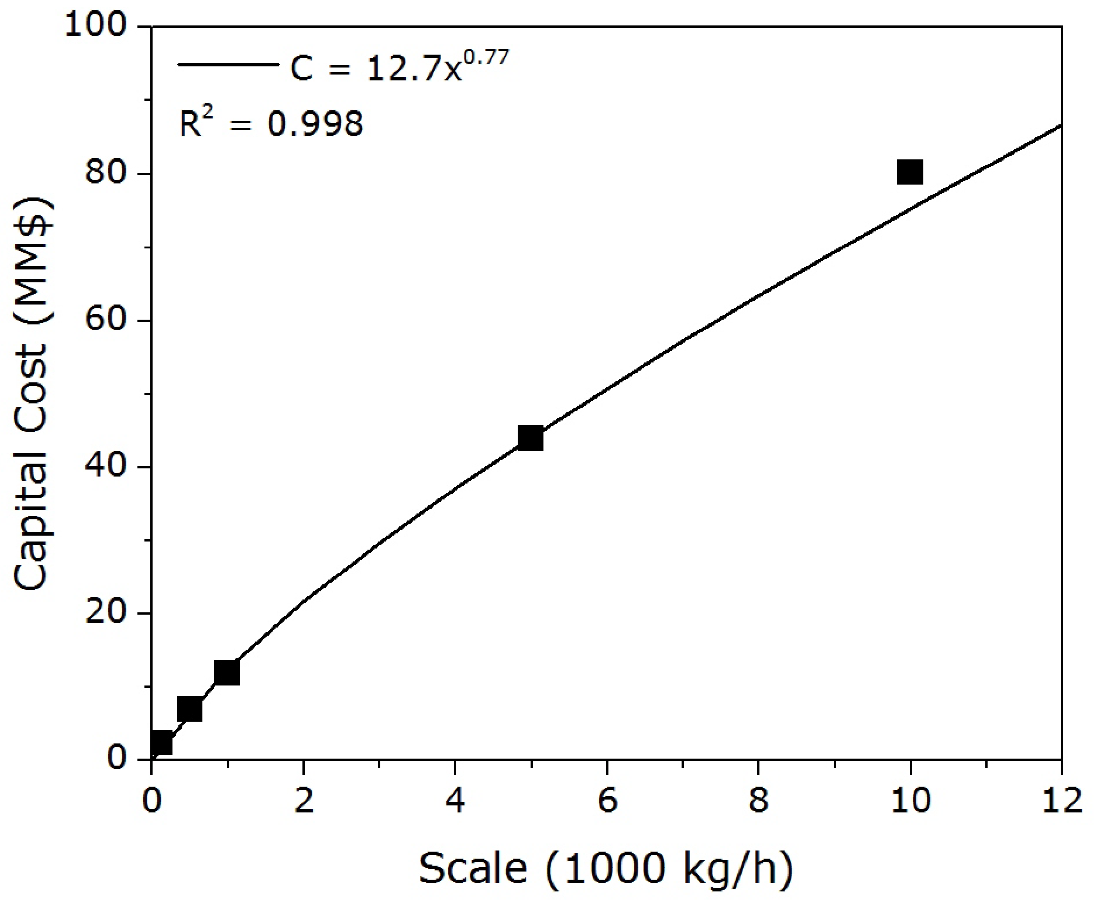
The optimal 20-year NPC and capital cost in millions of UDS (MM$) and specific energy consumption for each scale are given in

Table 9. Absorbent-enhanced ammonia synthesis optimal design results.

Scale, kgNH${}_3$/h	100	500	1000	5000	10,000
Net Present Cost, MM$	3.2	11.2	20.2	85.8	164.3
Capital Cost, MM$	2.3	7.0	11.8	43.9	80.2
Specific Energy Consumption, kWh/kgNH${}_3$	3.12	3.07	3.06	3.07	3.08

. In the chemical process industries, power law correlations are commonly used to relate the capital cost of entire processes at different scales [32]. A correlation of this type for the absorbent-enhanced process is fit to the five optimal capital cost data in Figure 2.

5.1. Analysis of Optimal Design

The following discussion provides a plausible physical explanation and justification for key aspects of the optimal design decisions, which are given in

Table 10. Absorbent-enhanced ammonia synthesis optimal design decisions.

Scale, kgNH${}_3$/h	100	500	1000	5000	10,000
Recycle Ratio	12.5	12.7	12.7	12.8	12.8
Reaction-Absorption Pressure, bar	20.3	20.3	20.3	20.3	20.3
Reactor Temperature, ${}^{\circ }$C	370	370	370	370	370
Reactor Length, m	1.48	2.68	3.52	7.68	10.68
Reactor Diameter, m	0.74	1.33	1.76	3.84	5.34
Heat Exchanger Area, m${}^2$	247	1250	2520	12,700	30,200
Absorber Temperature, ${}^{\circ }$C	167	174	176	178	176
Number of Absorber Tubes	4	29	68	512	1183
Absorber Tube Length, m	1.14	1.00	0.96	0.84	0.80
Absorber Tube Diameter, m	0.57	0.50	0.48	0.42	0.40
Trim Cooler Temperature, ${}^{\circ }$C	141	142	142	141	97
Desorption Pressure, bar	13.4	13.4	13.4	13.4	13.4
Desorption Temperature, ${}^{\circ }$C	500	500	500	500	500
Ammonia Compressor Precooler Temperature, ${}^{\circ }$C	57	50	48	43	42
Ammonia Storage Pressure, bar	23.4	21.2	20.5	19.1	18.6
Ammonia Storage Temperature, ${}^{\circ }$C	56	52	50	48	47

. Certain reaction-absorption loop characteristics, which are helpful in interpreting these results, are given in

Table 11. Reaction-absorption loop characteristics.

Scale, kgNH${}_3$/h	100	500	1000	5000	10,000
Reactor Volume, m${}^3$	0.64	3.72	8.58	88.6	239
Distance from Equilibrium, %	0.07	0.04	0.02	0.001	0.0001
Reactor Pressure Drop, bar	0.04	0.14	0.24	0.57	0.85
Total Pressure Drop, bar	1.23	1.11	1.12	1.28	1.50

.

The reaction-absorption pressure was 20.29 bar at all scales. This is the limiting pressure, which results in a feed compressor outlet temperature of 150 ${}^{\circ }$C. A higher reaction-absorption pressure would require multi-stage compression with inter-cooling for the feed, and the additional incurred cost would not be worth the increased reactor productivity resulting from the pressure increase.

The reactor inlet temperature was 370 ${}^{\circ }$C at all scales. This lowest allowable temperature shifts the reaction equilibrium towards ammonia, which, from a thermodynamic perspective, allows for the highest possible outlet mole fraction of ammonia at the given pressure. The combination of the recycle ratio and reactor dimensions at each scale takes advantage of the favorable equilibrium shift; it resulted in ammonia mole fractions at the reactor outlet of 4.5% to 4.6%, which is very close to equilibrium at reactor outlet conditions. It is clear that the optimal design maximized single-pass reactor productivity under the constraint of using only one feed compressor. The largest possible single-pass conversion corresponds to the smallest possible recycle rate, which serves to minimize recycle compression capital cost and energy consumption, both because power is a function of flow rate and specific work and because it minimizes the reaction-absorption loop pressure drop. Additionally, the lowest possible reaction temperature and recycle rates minimized the amount of cooling required after the reactor/before the absorber, which is the product of enthalpy (temperature) difference and flow rate, resulting in capital (smaller heat exchanger and cooler) and operating (less pumping of cooling water) cost savings.

The absorption temperature had a complex effect on the capital and operating cost of the process. A low absorption temperature decreased the equilibrium pressure, resulting in less ammonia leaving the absorber and therefore a lower recycle rate. It also reduced the demand on the trim cooler, which is needed after the absorber due to the temperature rise caused by the exothermic absorption. On the other hand, a high absorption temperature resulted in a lessened precooling demand, and more importantly, less heating was needed to move from the absorption temperature to the desorption temperature. From scales of 100 kg/h to 5000 kg/h, absorption temperature increased from 167 ${}^{\circ }$C to 178 ${}^{\circ }$C. This reflects the fact that a high absorption temperature primarily reduces the operating cost (less heating for desorption), which increases linearly with production rate, whereas a low absorption temperature primarily lowers capital cost (smaller recycle compressor), which scales up well in comparison. At these scales, the trim cooler outlet temperature was such that the recycle compressor reached 150 ${}^{\circ }$C. The optimal design at 10,000 kg/h does not follow the trend of the smaller scales. The absorption temperature in this case was 176 ${}^{\circ }$C, and the trim cooler temperature was 97 ${}^{\circ }$C, much lower than in the designs at other scales. This can be explained by the fact that the reaction-absorption loop pressure drop is higher at this scale (see Table 11), primarily due to the reactor pressure drop, so these lower temperatures were chosen to reduce the recycle compressor power: a lower absorption temperature gives a lower recycle rate, and compression power was linear in the inlet temperature (trim cooler temperature in this case).

As scale increases, the absorber was designed such that its pressure drop decreases; the factor by which the number of absorber tubes increases is greater than or equal to the factor by which the ammonia production scale increases. This occurs primarily because compressor cost (capacity exponent of 0.9) does not scale as well as absorber cost (capacity exponent of 0.68) and also to counteract the increase in reactor pressure drop with scale-up.

The desorption temperature was 500 ${}^{\circ }$C in all cases. This high temperature was chosen to give a high absorbent critical pressure. For example, the critical pressure of the absorbent at this temperature was 13.64 bar, whereas at 400 ${}^{\circ }$, the critical pressure was only 1.83 bar. This allows ammonia to leave the bed at a higher pressure and subsequently minimizes the size of the compressor required to bring the ammonia to storage pressure. At all scales, the ammonia compression capital and energy cost reduction that resulted outweighed the significant energy costs that came from this high desorption temperature. As the scale of ammonia production was increased, a decrease in ammonia storage pressure and temperature was observed; this serves to reduce the size and energy consumption of the ammonia compressor. This occurs because the cost of coolers and the condenser (capacity exponent of 0.71) scales better than compressor cost (capacity exponent of 0.9).

5.2. Analysis of Energy Consumption

The relative contribution of different unit types of the overall energy consumption is given in

Table 12. Operation type contribution to optimal energy consumption.

Operation	Value
Compression	0.16
Pumping cooling water	0.02
Desorption	0.82

. These fractions are the same at each scale under consideration.

It is evident that desorption was the dominant form of energy consumption. This is expected, given that conventional chemical processes often rely on combustion of fossil fuels to achieve high temperatures, but that is not an option in the wind-powered absorbent-enhanced process. On the other hand, it is promising that cooling used such a small fraction of the energy in this process; this supports the hypothesis that the higher separation temperatures afforded by using absorption instead of condensation are beneficial.

6. Discussion

The absorbent-enhanced ammonia synthesis capital cost correlation determined in this work is:

$$C^{cap}=12.7{(\frac{{\chi }_{N{H}_3}}{1000\mathrm{kg}/\mathrm{h}})}^{0.77}$$

(44)

where $C^{cap}$ is in MM$ and ${\chi }_{N{H}_3}$ is the ammonia production capacity in kg/h. This result compares well to those in the literature for small-scale Haber–Bosch processes. The ammonia supply chain optimization work in [10] uses the following capital cost correlation for a small-scale Haber–Bosch process [35]:

$$C^{cap}=1.482{(\frac{{\chi }_{N{H}_3}}{3\mathrm{kg}/\mathrm{h}})}^{0.67}$$

(45)

where $C^{cap}$ is in MM$ and ${\chi }_{N{H}_3}$ is the ammonia production capacity in kg/h. Comparing the correlation for the absorbent-enhanced process to this one, capital cost reductions of 86% at 100 kg/h to 78% at 10,000 kg/h are observed.

However, the Haber–Bosch cost correlation in [35] may be overly conservative based on the small size of the initial installation (only 3 kg/h). For another comparison at a more relevant reference scale, a mini Haber–Bosch unit with a capacity of 3 tons/day (125 kg/h) was quoted at 3.8 MM$ in [9]. In comparison, the absorbent-enhanced process would only cost 2.55 MM$ at that scale, a cost reduction of 33%. The 0.77 scaling exponent for the absorbent-enhanced process is higher than the conventional chemical industry exponent of 0.67, which suggests that this process is more well suited to implementation at a small scale. Conversely, this higher-than-average capacity exponent indicates that the absorbent-enhanced process may not scale up well. For example, if the 0.67 exponent is applied to the Haber–Bosch process using the process from [9] as the reference scale, this Haber–Bosch becomes less expensive than the absorbent enhanced process at a scale of 6075 kg/h (145 ton/day) and larger.

Although the capital cost of the absorbent enhanced process is lower than the Haber–Bosch one at a small scale, this is not true for energy consumption. The current optimal design of the absorbent-enhanced process uses between 3.06 and 3.12 kWh/kg NH${}_3$, whereas the process in [35] uses 2.12 kWh/kg NH${}_3$. At a larger scale, the 100 tons/day (4167 kg/h) Haber–Bosch process in [8] used only 0.64 kWh/kg NH${}_3$. This result is not entirely surprising, as the heating needed for desorption is very electricity-intensive. However, given that in the overall wind-to-ammonia pathway using electrolysis and PSA, electrolysis accounts for the majority of energy consumption (for example, 93% in [8]), the increased ammonia synthesis energy consumption may be worth the decrease in capital cost in the economic outlook of the overall system.

Additionally, the Haber–Bosch process has been optimized over a century, whereas this absorbent-enhanced process is novel, so there are avenues for further capital and operating cost reduction via process improvement. The key novelty in the process is the use of absorption rather than condensation to remove the ammonia from unreacted hydrogen and nitrogen, so naturally, the absorbent is the part of the process to which the most significant improvements can be made. In this work, absorbent capacity was estimated to be a ratio of 1 mol NH${}_3$ to 1 mol MgCl${}_2$ (5.6 kg of salt are needed to absorb 1 kg NH${}_3$) based on the work in [12]. Coupled with the fact that the salt only makes up 40% of the absorbent mixture, every absorbed kg of NH${}_3$ requires 14 kg of total absorbent. This results in large absorbent beds as compared to what is theoretically possible, which is absorbing 6 mol NH${}_3$ on 1 mol MgCl${}_2$ [25]. Efforts to increase the working capacity of these absorbents or to discover new ammonia absorbents with higher capacities will be beneficial in reducing process cost by reducing the size of absorbent beds and subsequently the pressure drop through the bed. Furthermore, the diameter of the currently-used absorbent pellets is on the order of 200 $\mathsf{\mu }$m [23], an order of magnitude smaller than what is conventionally used in industrial packed beds. As a result, many tubes of absorbent are required, especially at the larger scales under investigation, to prevent prohibitively high pressure drop. The design of larger absorbent pellets would almost certainly be beneficial in that some compromise between reduction in absorber size and recycle compression power could be achieved. An absorbent that can be regenerated at lower temperatures and/or with less temperature variation between absorption and desorption but still at pressures in the range of 15 bar would be beneficial given that desorption requires over 80% of the energy consumed in this process (see Table 12). Regeneration of this absorbent would require less energy consumption and, hence, reduce operating cost, without increasing the size (cost) of the compressor required to liquefy the ammonia, as is the case when the currently-used absorbent is regenerated at lower temperatures. Evidently, efforts to improve ammonia absorbent performance will significantly ameliorate the economics of this process.

Additional efforts to expand the understanding of ammonia synthesis kinetics would also be beneficial. It is clear that running the ammonia synthesis reaction at lower temperature is helpful at the low pressure of this process; the lower bound of 370 ${}^{\circ }$C was chosen as the reaction temperature at all scales. It is possible that an even lower reaction temperature would be beneficial, but a reliable low temperature ammonia synthesis kinetic expression does not currently exist in the literature. The study of ammonia synthesis at lower temperatures would aid in elucidating a true optimal reaction temperature and would perhaps lead to further capital cost and/or operating cost reduction.

References

- FAO. World Fertilizer Trends and Outlook to 2018; Annual Report 14; Food and Agriculture Organization of the United Nations (FAO): Rome, Italy, 2015; ISBN 978-92-5-108692-6. [Google Scholar]
- Smil, V. Enriching the Earth: Fritz Haber, Carl Bosch, and the Transformation of World Food Production; MIT Press: Massachusetts, MA, USA, 2004. [Google Scholar]
- Swaminathan, B.; Sukalac, K. Technology transfer and mitigation of climate change: The fertilizer industry perspective. In Proceedings of the IPCC Expert Meeting on Industrial Technology Development, Transfer and Diffusion, Tokyo, Japan, 21–23 September 2004. [Google Scholar]
- Rees, N.V.; Compton, R.G. Carbon-free energy: A review of ammonia-and hydrazine-based electrochemical fuel cells. Energy Environ. Sci. 2011, 4, 1255–1260. [Google Scholar] [CrossRef]
- Wang, G.; Mitsos, A.; Marquardt, W. Conceptual design of ammonia-based energy storage system: System design and time-invariant performance. AIChE J. 2017, 63, 1620–1637. [Google Scholar] [CrossRef] [Green Version]
- Reese, M.; Marquart, C.; Malmali, M.; Wagner, K.; Buchanan, E.; McCormick, A.; Cussler, E.L. Performance of a small-scale Haber process. Ind. Eng. Chem. Res. 2016, 55, 3742–3750. [Google Scholar] [CrossRef]
- Morgan, E.; Manwell, J.; McGowan, J. Wind-powered ammonia fuel production for remote islands: A case study. Renew. Energy 2014, 72, 51–61. [Google Scholar] [CrossRef]
- Morgan, E.R.; Manwell, J.F.; McGowan, J.G. Sustainable ammonia production from US offshore wind farms: A techno-economic review. ACS Sustain. Chem. Eng. 2017, 5, 9554–9567. [Google Scholar] [CrossRef]
- Bañares-Alcántara, R.; Dericks, G.; Fiaschetti, M.; Grünewald, P.; Lopez, J.M.; Tsang, E.; Yang, A.; Ye, L.; Zhao, S. Analysis of Islanded Ammonia-Based Energy Storage Systems; University of Oxford: Oxford, UK, 2015. [Google Scholar]
- Allman, A.; Daoutidis, P.; Tiffany, D.; Kelley, S. A framework for ammonia supply chain optimization incorporating conventional and renewable generation. AIChE J. 2017, 63, 4390–4402. [Google Scholar] [CrossRef]
- Wagner, K.; Malmali, M.; Smith, C.; McCormick, A.; Cussler, E.; Zhu, M.; Seaton, N.C. Column absorption for reproducible cyclic separation in small scale ammonia synthesis. AIChE J. 2017, 63, 3058–3068. [Google Scholar] [CrossRef]
- Malmali, M.; Le, G.; Hendrickson, J.; Prince, J.; McCormick, A.V.; Cussler, E.L. Better Absorbents for Ammonia Separation. ACS Sustain. Chem. Eng. 2018, 6, 6536–6546. [Google Scholar] [CrossRef]
- Malmali, M.; Wei, Y.; McCormick, A.; Cussler, E.L. Ammonia synthesis at reduced pressure via reactive separation. Ind. Eng. Chem. Res. 2016, 55, 8922–8932. [Google Scholar] [CrossRef]
- gPROMS ModelBuilder, version 5.1.1; Software for Advanced Process Modelling Platform; Process Systems Enterprise: London, UK, 2018.
- Multiflash, version 6.1; Software for PVT Modelling and Flow Assurance; KBC: Surrey, UK, 2017.
- Huber, M. (Ed.) NIST Thermophysical Properties of Hydrocarbon Mixtures Database (SUPERTRAPP); version 3.2; National Institute of Standards and Technology: Gaithersburg, MD, USA, 2007.
- Nielsen, A.; Kjaer, J.; Hansen, B. Rate equation and mechanism of ammonia synthesis at industrial conditions. J. Catal. 1964, 3, 68–79. [Google Scholar] [CrossRef]
- Liu, H. Ammonia Synthesis Catalysts: Innovation and Practice, 1st ed.; World Scientific: Singapore; Chemical Industry Press: Beijing, China, 2013. [Google Scholar]
- Dyson, D.; Simon, J. Kinetic expression with diffusion correction for ammonia synthesis on industrial catalyst. Ind. Eng. Chem. Fundam. 1968, 7, 605–610. [Google Scholar] [CrossRef]
- Wakao, N.; Funazkri, T. Effect of fluid dispersion coefficients on particle-to-fluid mass transfer coefficients in packed beds: Correlation of Sherwood numbers. Chem. Eng. Sci. 1978, 33, 1375–1384. [Google Scholar] [CrossRef]
- Specchia, V.; Baldi, G.; Sicardi, S. Heat transfer in packed bed reactors with one phase flow. Chem. Eng. Commun. 1980, 4, 361–380. [Google Scholar] [CrossRef]
- Shafeeyan, M.S.; Daud, W.M.A.W.; Shamiri, A. A review of mathematical modeling of fixed-bed columns for carbon dioxide adsorption. Chem. Eng. Res. Des. 2014, 92, 961–988. [Google Scholar] [CrossRef]
- Smith, C.; Malmali, M.M.; Liu, C.Y.; McCormick, A.; Cussler, E.L. Rates of Ammonia Absorption and Desorption in Calcium Chloride. ACS Sustain. Chem. 2018. submitted. [Google Scholar]
- Mofidi, S.A.H.; Udell, K.S. Study of heat and mass transfer in mgcl2/nh3 thermochemical batteries. J. Energy Resour. Technol. 2017, 139, 032005. [Google Scholar] [CrossRef]
- Sørensen, R.Z.; Hummelshøj, J.S.; Klerke, A.; Reves, J.B.; Vegge, T.; Nørskov, J.K.; Christensen, C.H. Indirect, reversible high-density hydrogen storage in compact metal ammine salts. J. Am. Chem. Soc. 2008, 130, 8660–8668. [Google Scholar] [CrossRef] [PubMed]
- Jinasena, A.; Lie, B.; Glemmestad, B. Dynamic Model of an Ammonia Synthesis Reactor Based on Open Information. In Proceedings of the 9th EUROSIM Congress on Modelling and Simulation, Oulu, Finland, 12–16 September 2016; pp. 943–948. [Google Scholar]
- Woods, D.R. Rules of Thumb in Engineering Practice, 1st ed.; Wiley-VCH: Weinheim, Germany, 2007. [Google Scholar]
- Chemical Engineering. Chemical Engineering Economic Indicators; Technical Report for Chemical Engineering; Chemical Engineering: Rockville, MD, USA, 2016. [Google Scholar]
- Committee of Stainless Steel Producers. Stainless Steel in Ammonia Production; Technical Report; American Iron and Steel Institute: Washington, DC, USA, 1978. [Google Scholar]
- Indicative Chemical Prices A-Z; 2006 Price for Magnesium Chloride; Independent Chemical Information Service: Sutton, UK, 2008.
- 717177 ALDRICH Silica Gel; 2018 Price for Technical Grade, Pore Size 60 A, 70-230 mesh, 63-200 μm Silica Gel; Millapore Sigma: Darmstadt, Germany, 2018.
- Towler, G.; Sinnott, R.K. Chemical Engineering Design: Principles, Practice and Economics of Plant and Process Design, 2nd ed.; Elsevier: New York, NY, USA, 2012. [Google Scholar]
- Ilas, A.; Ralon, P.; Rodriguez, A.; Taylor, M. Renewable Power Generation Costs in 2017; International Renewable Energy Agency: Masdar City, UAE, 2018. [Google Scholar]
- Lee, D.; Hochgreb, S. Hydrogen autoignition at pressures above the second explosion limit (0.6–4.0 MPa). Intern. J. Chem. Kinet. 1998, 30, 385–406. [Google Scholar] [CrossRef]
- Tiffany, D.; Reese, M.; Marquart, C. Economic Evaluation of Deploying Small to Moderate Scale Ammonia Production Plants in Minnesota Using Wind and Grid-Based Electrical Energy Sources; Technical Report; Minnesota Corn Research and Promotion Council: Shakopee, MN, USA, 2015. [Google Scholar]
Figure 1.
Absorbent-enhanced ammonia synthesis process flow diagram.
Figure 2.
Absorbent-enhanced ammonia synthesis capital cost power law.