Input Shaping Predictive Functional Control for Different Types of Challenging Dynamics Processes

Abstract

Predictive functional control (PFC) is a fast and effective controller that is widely used for processes with simple dynamics. This paper proposes some techniques for improving its reliability when applied to systems with more challenging dynamics, such as those with open-loop unstable poles, oscillatory modes, or integrating modes. One historical proposal considered is to eliminate or cancel the undesirable poles via input shaping of the predictions, but this approach is shown to sometimes result in relatively poor performance. Consequently, this paper proposes to shape these poles, rather than cancelling them, to further enhance the tuning, feasibility, and stability properties of PFC. The proposed modification is analysed and evaluated on several numerical examples and also a hardware application.

1. Introduction

Predictive functional control (PFC) is a simple controller that is effective for small-scale single-input-single-output (SISO) applications, especially for low-order and stable processes [1,2,3]. The main advantages of PFC compared to its prime competitor—that is, proportional integral derivative (PID)—are its ability to handle constraints and its transparent tuning parameters. Indeed, it must be emphasised that the performance of PFC should not be benchmarked against more advanced model predictive control (MPC) strategies [4], because the implementation is relatively much cheaper and requires only low computation with very straightforward coding [5,6].

Nevertheless, despite its apparently attractive benefits, PFC has received relatively little attention in the academic literature because of the lack of a priori stability guarantees [7,8], which are possible with more advanced MPC approaches. Consequently, several recent works have developed the basic concept of PFC to improve its overall tuning properties while providing a confident assurance in the resulting closed-loop performance and constraint handling [9,10,11,12]. However, most of these modifications perform well only with low-order and simple dynamical processes. For a system with open-loop unstable poles, significant underdamping, or integrating dynamics, PFC is quite challenging to tune effectively [13], and the resulting divergent or oscillating predictions may give rise to infeasibility and/or robustness issues.

PFC practitioners often deploy a type of cascade structure to handle a challenging dynamics process, where an inner loop is used to improve the dynamics for an outer loop to control [14,15]. This modification enables a user to retain an independent model (IM) structure that handles uncertainties, while retaining a similar tuning concept as the conventional approach. Nevertheless, the inner PFC can only accept a proportional-type controller to avoid any overcomplication when handling constraints [6]. This restriction makes it difficult to have a systematic selection of gain, rather than an ad hoc approach. Moreover, a back-calculation or anti-wind-up technique is required to avoid any saturation while satisfying the constraints [6], which also can be conservative and thus affect performance.

A fundamental conceptual weakness of a simplistic PFC approach is that one is basing decisions on an open-loop prediction, which may have undesirable, possibly divergent, dynamics; matching this to a desirable closed-loop dynamic will lead to an ill-posed approach. Hence, an alternative approach is to pre-stabilise/pre-shape the output predictions by shaping the future input dynamics so that the effect of unwanted poles on the predictions are alleviated or cancelled [16]. This modification can retain the systematic tuning concept of PFC, in addition to facilitating a recursive feasibility guarantee feature for constraint handling. However, the performance of this control law is not always desirable, since the cancellation of specified modes (poles) within the predictions using a minimal number of control input changes often requires an aggressive input trajectory [16,17,18], which is not implementable or ideal for some cases.

In practice, less aggressive shaping to remove the undesirable modes from the prediction [19] is preferable, and this forms the main thrust of the proposal in this paper. More specifically, the proposal here is that, rather than using a small, finite number of control moves (effectively, finite impulse response (FIR) parameterisation), such as in Generalized Predictive Control (GPC) Added the defination and conventional PFC, the future input moves will be parameterised using an infinite impulse response (IIR) instead. The preference for IIR over FIR is due to IIR being more convenient to manipulate and define than a high-order FIR, in general. In turn, by allowing the output modes to evolve over many more samples, the required input will be less aggressive. Nevertheless, due to the desire for simplicity and transparency that is a central tenet of PFC, in this paper, we choose not to generalise the parameterisation for different dynamics. Instead, this work seeks to provide some rigour on how to effectively and systematically shape the future input for a given dynamic and, moreover, how to ensure some recursive feasibility properties during constraint handling.

Section 2 of this paper presents a brief formulation of conventional PFC. Section 3 introduces the concept of input shaping PFC, together with the constraint handling approach. Section 4 demonstrate the proposed algorithms on several numerical examples and also on some laboratory hardware. Section 5 provides the conclusions.

2. Conventional PFC

This section presents, in brief, the main concepts, notation, and formulation of PFC, together with a systematic constraint handling approach. For more detailed derivations, theory, and concepts of PFC, an interested reader may refer to the references, e.g., [5,6,13,20]. Without loss of generality, a controlled autoregressive and integrated moving average (CARIMA)-based model is used instead of the standard independent model (IM) structure to derive the required unbiased predictions, as this form is more amenable to the algebra required to implement the shaping. Hence, the model will take the form:

$$a\left(z\right)y_k+b\left(z\right)u_k+\frac{{\zeta }_k}{\Delta \left(z\right)};\Delta \left(z\right)=1-z^{-1}$$

(1)

where $b\left(z\right)=b_1{z}^{-1}+...$ , $a\left(z\right)=1+a_1{z}^{-1}+...$, $y_k,u_k$ are the outputs and inputs, respectively, at sample k, and ${\zeta }_k$ is an unknown zero mean random variable used to capture uncertainty.

2.1. Control Law

PFC design is based on the assumption that a closed-loop response should follow a first-order dynamic from the current state $y_k$ to the desired target r [20]. In practice, one aims to achieve this by ensuring a matching using the open-loop prediction, but only at a single point. In other words, the predicted output trajectory is chosen to satisfy the following equality:

$$y_{k+n|k}=(1-{\lambda }^n)r+{\lambda }^n{y}_k$$

(2)

where $y_{k+n_y|k}$ is the n-step ahead system prediction at sample time k, and $\lambda$ is the desired closed-loop pole that will determine the speed of convergence. PFC practitioners typically select the desired closed-loop time response (CLTR) which has an explicit link with the corresponding closed-loop pole, that is, $\lambda =e^{\frac{-3T}{CLTR}}$, where T is the sampling period [6].

The predictions for the CARIMA model (1) are standard in the literature (e.g., [4,21]), so only the final form is given here. For input increments $\Delta u_{k+i}$, the n-step ahead future output prediction is formed as:

$${\stackrel{{\displaystyle y}}{\to }}_{k+1|k}=H\stackrel{{\displaystyle \Delta u_k}}{\to }+P\stackrel{{\displaystyle \Delta u_k}}{\leftarrow }+Q\stackrel{{\displaystyle y_k}}{\leftarrow }$$

(3)

where the left and right arrow underlying vectors represent past and future variables, respectively. The parameters H, P, Q depend on the model parameters, and for a model of order m:

$$\Delta \stackrel{{\displaystyle u_k}}{\to }=\left[\begin{array}{c}\Delta u_k\hfill \\ \Delta u_{k+1}\hfill \\ ⋮\hfill \\ \Delta u_{k+n-1}\hfill \end{array}\right];\stackrel{{\displaystyle \Delta u_k}}{\leftarrow }=\left[\begin{array}{c}\Delta u_{k-1}\\ \Delta u_{k-2}\\ ⋮\\ \Delta u_{k-m}\end{array}\right];\stackrel{{\displaystyle y_k}}{\leftarrow }=\left[\begin{array}{c}{y}_k\hfill \\ y_{k-1}\hfill \\ ⋮\hfill \\ y_{k-m}\hfill \end{array}\right];{\stackrel{{\displaystyle y}}{\to }}_{k+1|k}=\left[\begin{array}{c}{y}_{k+1}\\ y_{k+2}\\ ⋮\\ y_{k+n}\end{array}\right]$$

(4)

In conventional PFC [6,20], within the predictions we select $\Delta u_{k+i}=0,i>0$. Uusing this and substituting the n-step ahead prediction from (3) into equality (2) gives:

$$H_n{\mathbf{e}}_1\Delta u_k+P_n\stackrel{{\displaystyle \Delta u_k}}{\leftarrow }+Q_n\stackrel{{\displaystyle y_k}}{\leftarrow }=(1-{\lambda }^n)r+{\lambda }^n{y}_k$$

(5)

where ${\mathbf{e}}_i$ is the ith standard basic vector and $H_n={\mathbf{e}}_n^{T}H,P_n={\mathbf{e}}_n^{T}P,Q_n={\mathbf{e}}_n^{T}Q$. Hence, the PFC control law is given as:

$$\Delta u_k=\frac{1}{h_n}\left[(1-{\lambda }^n)r+{\lambda }^n{y}_k-Q_n\stackrel{{\displaystyle y_k}}{\leftarrow }-P_n\stackrel{{\displaystyle \Delta u_k}}{\leftarrow }\right];h_n=H_n{\mathbf{e}}_1$$

(6)

Remark 1.

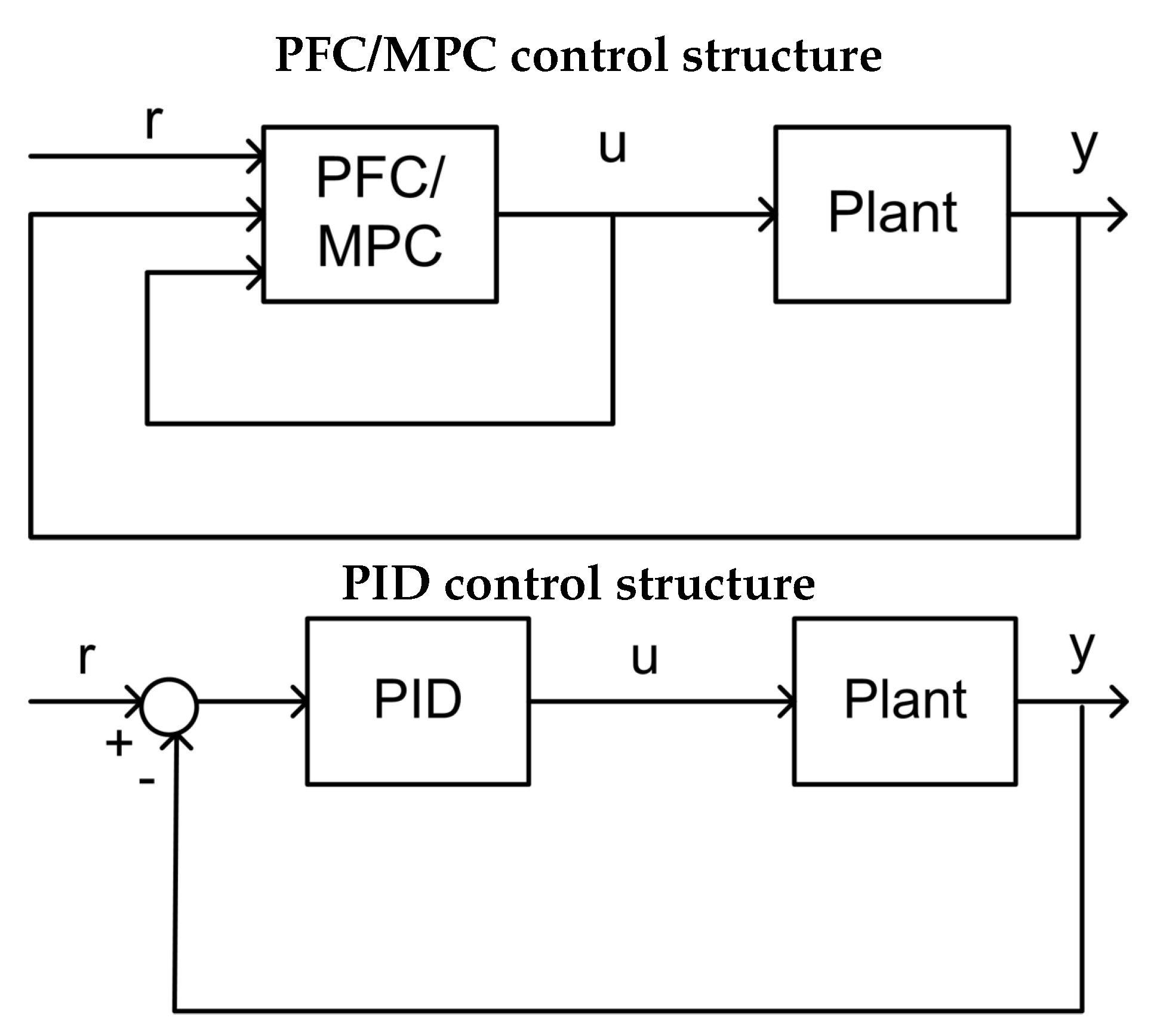
Figure 1 shows a comparison of simplified flow diagrams, where both PFC and MPC share the same structure, yet have a different optimisation process, where the constraint handling is embedded inside the main block. As for PID, the control input is obtained simply by tuning the gains, while the constraints are handled via a rule base [22].

Remark 2.

It is noted that PFC performs well for a system with close to a monotonic step response, such as a first-order system and overdamped second-order dynamics, assuming, of course, a sensible choice of the tuning parameters λ and n [11,12,13]. However, the same tuning procedure may not work for systems with less simple open-loop dynamics, leading to ill-posed decision making and unreliable control.

2.2. Constraint Handling

The constraint handling approach presented here is adapted from the standard MPC literature [21,23] but with simpler code, and it is more systematic and less conservative than the back-calculation typically used in conventional PFC algorithms [24]. Similarly, it will be more efficient than the ad hoc approaches used with PID. Assume constraints, at every sample, on input rate, input, and states, as follows:

$$\underline{\Delta u}\le \Delta u_k\le \overline{\Delta u};\underline{u}\le u_k\le \overline{u};\underline{y}\le y_k\le \overline{y},\forall k$$

(7)

The user needs to:

• Find a suitable horizon m [23] over which to compute the entire set of future output predictions in a single vector: ${\stackrel{{\displaystyle y}}{\to }}_{k+1|k}=H{\mathbf{e}}_{\mathbf{1}}\Delta u_k+P\stackrel{{\displaystyle \Delta u_k}}{\leftarrow }+Q\stackrel{{\displaystyle y_k}}{\leftarrow }$. The horizon for output predictions ${\stackrel{{\displaystyle y}}{\to }}_{k+1}$, and thus the row dimension of H, should be long enough to capture all core dynamics!
• Combine the input constraints, rate constraints, and output predictions into a single set of linear inequalities:

  $$C\Delta u_k\le {\mathbf{f}}_k$$

  (8)

  $$C=\left[\begin{array}{c}1\\ -1\\ 1\\ -1\\ H{\mathbf{e}}_{\mathbf{1}}\\ -H{\mathbf{e}}_{\mathbf{1}}\end{array}\right];{\mathbf{f}}_k=\left[\begin{array}{c}\overline{u}-u_{k-1}\\ -\underline{u}+u_{k-1}\\ \overline{\Delta u}\\ -\underline{\Delta u}\\ L\overline{y}-P\stackrel{{\displaystyle \Delta u_k}}{\leftarrow }-Q\stackrel{{\displaystyle y_k}}{\leftarrow }\\ -L\underline{y}+P\stackrel{{\displaystyle \Delta u_k}}{\leftarrow }+Q\stackrel{{\displaystyle y_k}}{\leftarrow }\end{array}\right];L=\left[\begin{array}{c}1\\ 1\\ ⋮\\ 1\end{array}\right]$$

  where ${\mathbf{f}}_k$ depends on past data in $\stackrel{{\displaystyle \Delta u_k}}{\leftarrow },\stackrel{{\displaystyle y_k}}{\leftarrow }$ and on the limits.
• The input/output predictions will satisfy constraints if inequalities (8) are satisfied, and thus the PFC algorithm should consider these explicitly.

Next, a single simple loop is utilised to find the $\Delta u_k$ closest to the unconstrained solution of (6), while satisfying (8).

Algorithm 1. Simple PFC algorithm with systematic constraint handling

At each sample:    Define the unconstrained value for $\Delta u_k$ from (6).  Define the vector ${\mathbf{f}}_k$ of (8) (it is noted that C does not change).  Use a simple loop covering all the rows of C as follows: (a)   Check the ith constraint that is the ith row ${\mathbf{e}}_i^{T}C\Delta u_k\le {\mathbf{f}}_{k,i}$ of $C\Delta u_k\le {\mathbf{f}}_k$. (b)   If ${\mathbf{e}}_i^{T}C\Delta u_k>f_{k,i}$, then set $\Delta u_k=\left(f_{k,i}\right)/\left[{\mathbf{e}}_i^{T}C\right]$, else leave $\Delta u_k$ unchanged.

Remark 3.

For a simple and stable open-loop process and for suitably large m, Algorithm 1 is guaranteed to be recursively feasible and, moreover, to converge to a possible value for $\Delta u_k$ that is closest to the unconstrained choice [12]. However, this benefit does not apply to systems with more challenging dynamics, such as when the open-loop prediction is divergent.

3. Input Shaping PFC

This section presents the concept of input shaping to pre-stabilise (or pre-condition) the open-loop predictions of processes with undesirable dynamics. The shaping of input predictions can be done either via explicit pole cancellation or pole shaping, and both methods can be used to formulate a PFC control law which retains a recursively feasible constrained solution. A key issue, however, is whether one deploys FIR or IIR parameterisations of the predictions for the future input increments $\Delta u_{k+i|k},i\ge 0$.

3.1. Pre-Stabilisation of Predictions via Pole Cancellation

For systems with poor open-loop dynamics, the constant input assumption of typical PFC does not provide enough flexibility within the predicted input to both cancel the effect of an undesirable pole and to get nice convergent behaviour [13,17,19]. Thus, it is crucial to first stabilise the prediction before implementing it into a control law [25]. The first step is to factorise the poles in the denominator:

$$\Delta y\left(z\right)=\frac{b\left(z\right)}{a\left(z\right)}\Delta u\left(z\right);a\left(z\right)=a^{-}\left(z\right)a^{+}\left(z\right)$$

(9)

where $a^{+}\left(z\right)$ contains the undesirable poles. Utilising the Toeplitz/Hankel form [21], the future output predictions can be computed as:

$$\left[C_{a^{-}\Delta }\right]\left[C_{a^{+}}\right]{\stackrel{{\displaystyle y}}{\to }}_{k+1}+H_A{\stackrel{{\displaystyle y}}{\leftarrow }}_k=C_b\Delta {\stackrel{{\displaystyle u}}{\to }}_k+H_b\Delta {\stackrel{{\displaystyle u}}{\leftarrow }}_k$$

(10)

where for general polynomial $f\left(z\right)=f_0+f_1{z}^{-1}+...+f_n{z}^{-n}$,

$$C_f=\left[\begin{array}{cccc}{f}_0& 0& 0& ...\\ f_1& f_0& 0& ...\\ ⋮& ⋮& ⋮& \ddots \\ f_n& f_{n-1}& f_{n-2}& ...\end{array}\right];H_f=\left[\begin{array}{cccc}{f}_1& f_2& ...& f_n\\ f_2& f_2& ...& 0\\ ⋮& ⋮& ⋮& \ddots \\ 0& 0& ...& 0\end{array}\right]$$

Rearranging prediction (10) in more compact form, we get:

$${\stackrel{{\displaystyle y}}{\to }}_{k+1}={[C_{a^{-}\Delta }]}^{-1}{[C_{a^{+}}]}^{-1}[C_b\Delta {\stackrel{{\displaystyle u}}{\to }}_k+\underset{\mathbf{p}}{\underbrace{H_b\Delta {\stackrel{{\displaystyle u}}{\leftarrow }}_k-H_A{\stackrel{{\displaystyle y}}{\leftarrow }}_k}}]$$

(11)

from which the presence of the undesirable modes are transparent through the factor ${\left[C_{a^{+}}\right]}^{-1}$.

Lemma 1.

Selection of the future input sequence $\Delta {\stackrel{{\displaystyle u}}{\to }}_k$, at each sample, such that the following equality is satisfied:

$$[C_b\Delta {\stackrel{{\displaystyle u}}{\to }}_k+\mathbf{p}]=C_{a^{+}}\gamma$$

(12)

where γ is a convergent sequence or a polynomial, will ensure that the corresponding output predictions in (11) do not contain the undesirable modes in $a^{+}$.

Proof. 

This is self-evident by substitution of (12) into (11), which gives:

$${\stackrel{{\displaystyle y}}{\to }}_{k+1}={\left[C_{a^{-}\Delta }\right]}^{-1}{\left[C_{a^{+}}\right]}^{-1}\left[C_{a^{+}}\right]\gamma ={\left[C_{a^{-}\Delta }\right]}^{-1}\gamma$$

(13)

so that only the acceptable modes in $a^{-}\left(z\right)$ remain in the predictions, along with any components in the convergent sequence $\gamma$. It is noted that this choice automatically includes the initial conditions within $\mathbf{p}$ and thus updates each sample as required. □

Remark 4.

Requirement (12) can be solved by a small number of simultaneous equations [21], where the minimal-order solution can be represented as:

$$\Delta {\stackrel{{\displaystyle u}}{\to }}_k=P_1\mathbf{p};\gamma =P_2\mathbf{p}$$

(14)

for suitable $P_1,P_2$. The required dimension of non-zero elements in vector $\Delta {\stackrel{{\displaystyle u}}{\to }}_k$ corresponds to at least one more than the number of undesirable modes ($n_{a^{+}}$), while the order of γ is usually taken as $n_{\gamma }=n_p-n_{a^{+}}$, where $n_p$ is the effective dimension of $\mathbf{p}$ (which depends upon the column dimensions of $H_b,H_A$).

To ensure the future manipulated control moves are convergent, while adding some flexibility for modifying the output predictions, the input requirement in (14) can be enhanced to:

$$\Delta {\stackrel{{\displaystyle u}}{\to }}_k=P_1\mathbf{p}+C_{a^{+}}\varphi$$

(15)

where the vector parameter $\varphi$ denotes the degrees of freedom (d.o.f.) within the predictions.

Theorem 1.

Using the new shaped input (15) ensures that the undesirable modes do not appear in the output predictions, irrespective of the choice of ϕ. The output predictions are convergent if ϕ is finite-dimensional or a convergent infinite dimensional sequence.

Proof. 

Substitute input prediction (15) into output prediction (12), and the predictions become:

$$\begin{array}{cc}\hfill {\stackrel{{\displaystyle y}}{\to }}_{k+1}& ={\left[C_{a^{-}\Delta }\right]}^{-1}{\left[C_{a^{+}}\right]}^{-1}[C_b\Delta {\stackrel{{\displaystyle u}}{\to }}_k+\mathbf{p}]\hfill \\ & ={\left[C_{a^{-}\Delta }\right]}^{-1}{\left[C_{a^{+}}\right]}^{-1}[C_{a^{+}}\gamma +C_b{C}_{a^{+}}\varphi ]\hfill \\ & ={\left[C_{a^{-}\Delta }\right]}^{-1}[C_b\varphi +\gamma ]\hfill \end{array}$$

(16)

The prediction can be represented with an equivalent z-transform:

$$\stackrel{{\displaystyle y}}{\to }\left(z\right)=\frac{[1,z^{-1},z^{-2},\cdots ][\gamma +C_b\varphi ]}{a^{-}\left(z\right)}=\frac{\gamma \left(z\right)+b\left(z\right)\varphi \left(z\right)}{a^{-}\left(z\right)}$$

(17)

It is known from Lemma 1 that the contribution from $\gamma$ gives a convergent prediction, and thus overall convergence is obvious as long as $\varphi \left(z\right)$ is convergent (or an FIR). □

Remark 5.

Noting the definition of $\mathbf{p}$ in (11), the n-step ahead output prediction with prediction class (15) and (17) can be put in a more common form as:

$$y_{k+n|k}=H_{s,n}\varphi +P_{s,n}\stackrel{{\displaystyle \Delta u_k}}{\leftarrow }+Q_{s,n}\stackrel{{\displaystyle y_k}}{\leftarrow }$$

(18)

where $H_{s,n}$, $P_{s,n}$, and $Q_{s,n}$ are suitable matrices, and the additional subscript ‘s’ is used to denote shaping and ϕ is taken to be FIR (equivalently a finite dimensional vector). Note, however, that typically for PFC, ϕ is a scalar. Also, it is easy to show [18] that choosing $\varphi =0$ will automatically give the same input predictions as those deployed at the previous sample, which enables consistency of predictions from one sample to the next.

3.2. Pre-Stabilisation via Pole Shaping

It is known that dead-beat pole cancellation can require aggressive inputs, and the minimal-order solutions to (12) are in effect dead-beat input predictions [16,19]. Although dead-beat solutions are easy to define and thus have some advantages in terms of computation and transparency, in practice, a user may desire a less aggressive shaping that is more implementable in a real system. Alongside this, the popularity of dual mode approaches in the literature [26] is partially because they allow the implied input predictions to converge to the steady state asymptotically, rather than in a small, finite number of steps. Thus, a logical question to ask is whether a smoother solution to (12)—that is, one where the implied solutions for $\gamma \left(z\right),\varphi \left(z\right)$ used in (17) have some poles, say $\alpha \left(z\right)$—would work better for PFC.

The mainstream MPC community has focussed on optimal control solutions, but, given that PFC is intended to be simple and low-dimensional, the proposal here is that it is more reasonable to investigate the potential of simple default choices for the asymptotic dynamics $\alpha \left(z\right)$ within the input and output predictions. Clearly, this choice can be strongly linked to the target closed-loop behaviour and/or system knowledge.

Proposal 1.

By definition, the integrator has a pole on the unit circle—that is, factor $(1-z^{-1})$—and, conversely, cancelling the pole as in (12) is equivalent to enforcing a pole on the origin—that is, factor $(1-0$ $z^{-1})$. Hence, the choice of pole factor $\alpha =(1-0.5$ $z^{-1})$ represents a simple half-way house trade-off between these two choices.

Proposal 2.

For a process with significant underdamping, the implied $\alpha \left(z\right)$ will have only real poles which are chosen to be close to the real parts of the oscillatory poles. This will reduce the undesirable oscillation in the output predictions, but not change the convergence speed, albeit the input may then be somewhat oscillatory.

Proposal 3.

For open-loop unstable systems, a simple default solution simply inverts the unstable poles, that is, defining $\alpha \left(z\right)$ such that $a^{+}\left(z_i\right)=0\Rightarrow \alpha (1/z_i)=0$.

Lemma 2.

The dynamics $\alpha \left(z\right)$ will be present in the predictions if the following Diophantine equation is used to solve the input/output prediction pairing.

$$b\left(z\right)w\left(z\right)+\alpha \left(z\right)p\left(z\right)=a^{+}\left(z\right)\widehat{\gamma }\left(z\right);p\left(z\right)=[1,z^{-1},...]\mathbf{p}$$

(19)

$$\Rightarrow \Delta \stackrel{{\displaystyle u}}{\to }\left(z\right)=\frac{w\left(z\right)}{\alpha \left(z\right)},\stackrel{{\displaystyle y}}{\to }\left(z\right)=\frac{\widehat{\gamma }\left(z\right)}{a^{-}\left(z\right)\Delta \left(z\right)\alpha \left(z\right)}$$

Proof. 

First, note that (19) is equivalent to solving:

$$[C_b{C}_{\alpha }^{-1}\mathbf{w}+\mathbf{p}]=C_{a^{+}}{C}_{\alpha }^{-1}\widehat{\gamma }$$

(20)

and, moreover, Equation (20) follows directly from enforcing (12) while assuming $\Delta {-1.1ex\stackrel{{\displaystyle u}}{\to }}_k=C_{\alpha }^{-1}\mathbf{w}$. Hence, substituting this $\Delta {\stackrel{{\displaystyle u}}{\to }}_k$ into (11) gives:

$$\begin{array}{cc}{\stackrel{{\displaystyle y}}{\to }}_{k+1}\hfill & ={\left[C_{a^{-}\Delta }\right]}^{-1}{\left[C_{a^{+}}\right]}^{-1}[C_b\Delta {\stackrel{{\displaystyle u}}{\to }}_k+\mathbf{p}]\hfill \\ & ={\left[C_{a^{-}\Delta }\right]}^{-1}{\left[C_{a^{+}}\right]}^{-1}[C_b{C}_{\alpha }^{-1}\mathbf{w}+\mathbf{p}]\hfill \\ & ={\left[C_{a^{-}\Delta }\right]}^{-1}{\left[C_{a^{+}}\right]}^{-1}\left[C_{a^{+}}{C}_{\alpha }^{-1}\widehat{\gamma }\right]=C_{a^{-}\Delta }^{-1}{C}_{\alpha }^{-1}\widehat{\gamma }\hfill \end{array}$$

(21)

It is evident, therefore, that the desired poles are in the predictions for both the input and output. □

Remark 6.

The new requirement (20) can be solved similarly to (12), where the minimal-order solution for $\mathbf{w}$ and $\widehat{\gamma }$ are:

$$\mathbf{w}=\widehat{P_1}\mathbf{p};\widehat{\gamma }=\widehat{P_2}\mathbf{p}$$

(22)

Theorem 2.

A convergent prediction class which embeds both the desired asymptotic poles and some degrees of freedom (d.o.f.) can be defined from:

$$\mathbf{w}=\widehat{P_1}\mathbf{p}+C_{a^{+}}\varphi ;\Delta {\stackrel{{\displaystyle u}}{\to }}_k={\left[C_{\alpha }\right]}^{-1}[\widehat{P_1}\mathbf{p}+C_{a^{+}}\varphi ]$$

(23)

where convergent IIR or FIR ϕ constitutes the d.o.f.

Proof. 

This is analogous to Theorem 1 and is based on superposition. The additional component in $\mathbf{w}$—that is, $C_{a^{+}}\varphi$—necessarily cancels the undesirable poles and gives overall convergent output predictions. So, using (21), then: Added hat on top of gamma in Equation (24).

$$\begin{array}{cc}\hfill {\stackrel{{\displaystyle y}}{\to }}_{k+1}& =C_{a^{-}\Delta }^{-1}{C}_{a^{+}}^{-1}[C_b\Delta {\stackrel{{\displaystyle u}}{\to }}_k+\mathbf{p}]\hfill \\ & =C_{a^{-}\Delta }^{-1}{C}_{\alpha }^{-1}\widehat{\gamma }+C_{a^{-}\Delta }^{-1}{C}_{a^{+}}^{-1}{C}_{\alpha }^{-1}\left[C_{a^{+}}{C}_b\varphi \right]\hfill \\ & =C_{a^{-}\Delta }^{-1}{C}_{\alpha }^{-1}[\widehat{\gamma }+C_b\varphi ]\hfill \end{array}$$

(24)

□

Remark 7.

By extracting the $n^{th}$ row and noting the definition of $\mathbf{p}$ in (11), the n-step ahead prediction from (24) can be rearranged in a more general form as:

$$y_{k+n|k}=h_{n,\alpha }\varphi +P_{n,\alpha }\stackrel{{\displaystyle \Delta u_k}}{\leftarrow }+Q_{n,\alpha }\stackrel{{\displaystyle y_k}}{\leftarrow }$$

(25)

for suitable $h_{n,\alpha },P_{n,\alpha },Q_{n,\alpha }$, and it is noted that as is conventional for PFC, ϕ has just a single non-zero parameter in order to retain computational simplicity and to have just a single d.o.f. for satisfying the control law (2).

3.3. Proposed Shaping PFC Control Laws

Since the shaped predictions of (18) and (25) are derived in a general form, two new control laws—Pole Cancellation PFC (PC-PFC) and Pole Shaping PFC (PS-PFC)—can be formulated in a conventional manner after selecting a suitable coincidence horizon n and desired closed-loop pole $\lambda$.

[PC-PFC] The d.o.f $\varphi$ is computed by substituting prediction (18) of PC-PFC into equality (2), and thus:

$$\varphi =\frac{1}{h_{n,s}}\left[(1-{\lambda }^n)r+{\lambda }^n{y}_k-Q_{n,s}\stackrel{{\displaystyle y_k}}{\leftarrow }-P_{n,s}\stackrel{{\displaystyle \Delta u_k}}{\leftarrow }\right]$$

(26)

then, the current input increment $\Delta u_k$ is determined simply by inserting $\varphi$ into the predicted input of (15).

[PS-PFC] The d.o.f $\varphi$ is computed by substituting prediction (25) of PS-PFC into equality (2), and thus:

$$\varphi =\frac{1}{h_{n,\alpha }}\left[(1-{\lambda }^n)r+{\lambda }^n{y}_k-Q_{n,\alpha }\stackrel{{\displaystyle y_k}}{\leftarrow }-P_{n,\alpha }\stackrel{{\displaystyle \Delta u_k}}{\leftarrow }\right]$$

(27)

then, the current input increment $\Delta u_k$ is determined simply by inserting $\varphi$ into the predicted input of (23).

3.4. Constraint Handling Approaches with Recursive Feasibility

A core advantage of MPC, in general, is that the optimised predictions can be restricted to ones which satisfy constraints; the d.o.f. within the predictions are used to ensure constraint satisfaction. For PC-PFC and PS-PFC, the d.o.f. in the predictions is the variable $\varphi$. This section gives a brief overview of how the constraint inequalities ensuring (7) depend upon $\varphi$. We will use PS-PFC and assume that the reader can easily find the equivalent matrices for PC-PFC (for which, in effect, $\alpha =1$).

Noting the definition of future input increments in (23) and output predictions in (25), the constraints inequalities for (7) can be defined as:

$$\begin{array}{cc}\hfill L\underline{\Delta u}& \le C_{\alpha }^{-1}[\widehat{P_1}\mathbf{p}+C_{a^{+}}\varphi ]\le L\overline{\Delta u};\hfill \\ \hfill L\underline{u}& \le C_{I/\Delta }{C}_{\alpha }^{-1}[\widehat{P_1}\mathbf{p}+C_{a^{+}}\varphi ]+L{u}_{k-1}\le L\overline{u};\hfill \\ \hfill L\underline{y}& \le H_{\alpha }\varphi +P_{\alpha }\stackrel{{\displaystyle \Delta u_k}}{\leftarrow }+Q_{\alpha }\stackrel{{\displaystyle y_k}}{\leftarrow }\le L\overline{y}.\hfill \end{array}$$

(28)

where $C_{I/\Delta }$ is a lower triangular matrix one ones, and L is a vector of ones with an appropriate dimension (typically a horizon long enough to capture the core dynamics in the predictions). The reader should note that the horizon for the predictions used in (28) will, in general, be much longer than the coincidence horizon used in (27), as one needs to ensure that the implied long-range predictions satisfy constraints. The inequalities can be combined for convenience as follows, although this is not necessary for online coding where efficient alternatives may exist:

$$C\varphi \le {\mathbf{f}}_k$$

(29)

$$C=\left[\begin{array}{c}{C}_{I/\Delta }{C}_{\alpha }^{-1}{C}_{a^{+}}\\ -C_{I/\Delta }{C}_{\alpha }^{-1}{C}_{a^{+}}\\ C_{\alpha }^{-1}{C}_{a^{+}}\\ -C_{\alpha }^{-1}{C}_{a^{+}}\\ H_{\alpha }\\ -H_{\alpha }\end{array}\right];{\mathbf{f}}_k=\left[\begin{array}{c}L[\overline{u}-u_{k-1}]-C_{I/\Delta }{C}_{\alpha }^{-1}\widehat{P_1}\mathbf{p}\\ L[-\underline{u}+u_{k-1}]+C_{I/\Delta }{C}_{\alpha }^{-1}\widehat{P_1}\mathbf{p}\\ L\overline{\Delta u}-C_{\alpha }^{-1}\widehat{P_1}\mathbf{p}\\ -L\underline{\Delta u}+C_{\alpha }^{-1}\widehat{P_1}\mathbf{p}\\ L\overline{y}-P_{\alpha }\stackrel{{\displaystyle \Delta u_k}}{\leftarrow }-Q_{\alpha }\stackrel{{\displaystyle y_k}}{\leftarrow }\\ -L\underline{y}+P_{\alpha }\stackrel{{\displaystyle \Delta u_k}}{\leftarrow }+Q_{\alpha }\stackrel{{\displaystyle y_k}}{\leftarrow }\end{array}\right]$$

Algorithm 2. [PS-PFC with constraint handling]

At each sample:    Define the unconstrained value for ϕ from (27).  Update the vector ${\mathbf{f}}_k$ of (29) (it is noted that C does not change).  Use a simple loop covering all the rows of C as follows: (a)  Check satisfaction of the ith constraint using: ${\mathbf{e}}_i^{T}C\varphi \le f_{k,i}$. (b)  If ${\mathbf{e}}_i^{T}C\varphi >f_{k,i}$, then set $\varphi =\left(f_{k,i}\right)/\left[{\mathbf{e}}_i^{T}C\right]$, else leave ϕ unchanged.

Theorem 3.

In the presence of constraints, Algorithm 2 is recursively feasible where the computed ϕ will not only enforce the input/output predictions to satisfy constraints at the current sample, but will also guarantee that one can make the same statement at the next sample.

Proof. 

By definition, the choice of $\varphi =0$ ensures feasibility in the nominal case because the input component $\widehat{P_1}\mathbf{p}$ is the unused part of the input prediction from the previous sample, and this is known to satisfy constraints by assumption. One can ensure feasibility at start-up by beginning from a sensible state. □

Readers should note that using the pre-stabilised/shaped predictions is essential for this recursive feasibility result, which is not available for more conventional PFC approaches, for which the implied long-range predictions may be divergent. Thus, this Theorem is an important contribution of this paper.

Remark 8.

Although Algorithm 2 allows recursive feasibility, which is a strong result, ironically, the use of PC-PFC or PS-PFC does not not give any a priori stability and/or performance guarantees in general, which is a well-understood weakness of PFC approaches [7] and a consequence of wanting a very simple and cheap control approach.

4. Numerical Examples

This section presents several numerical examples of the proposed Pole Shaping PFC (PS-PFC) in handling different types of challenging dynamics, while comparing its performance with the Pole Cancellation PFC (PC-PFC) and conventional PFC (PFC). These examples will highlight:

• the impact of input shaping on the open-loop behaviour;
• the trade-off in the closed-loop performance;
• the efficacy of constraint handling;
• the efficacy on laboratory hardware.

For demonstration purposes, the first three processes with varying dynamics are investigated in a MATLAB simulation environment in Section 4.1, Section 4.2, Section 4.3 and Section 4.4. The final example in Section 4.5 is on laboratory hardware.

4.1. Description of Case Studies

The case studies presented here are inspired from the real process applications. However, for clarity of presentation, the model parameters are not specific to a given piece of apparatus, but rather are generic to attain suitable dynamics which enable an explicit comparison between the control laws. In this work, it is assumed that there is no plant model mismatch. The robustness properties of these controllers will remain as future work, although it is noted that, as with most predictive controllers, disturbance rejection and offset free tracking is implicit.

4.1.1. Case Study 1: Boiler Level Control

In the process industry, the use of a boiler is frequent, and the level of water needs to be controlled within the manufacturer’s specified limits. Exceeding the allowable limits may lead to water overflow, overheating, and/or damage to many components. Conversely, if the level is low, the water wall tubes may overheat and cause tube ruptures, resulting in expensive repairs and other potential hazards. Hence, the prime control objective is to raise the water level at the boiler start-up point while retaining it at a constant steam load. Since the conversion process from water to steam is very slow, a typical model for this process is usually a first-order system with an integrator and stable zero [27]. In a discrete form, one of the poles should reside in a unit circle. The relationship between the output water level (m), $y\left(z\right)$, and the input water flow rate (${\mathrm{m}}^3$${\mathrm{s}}^{-1}$), $u\left(z\right)$, can be represented by a representative model, such as $G_1$:

$$G_1=\frac{0.1z^{-1}+0.4z^{-2}}{(1-0.8z^{-1})(1-z^{-1})}$$

(30)

4.1.2. Case Study 2: Depth Control of Unmanned Free-Swimming Submersible (UFSS)

In the marine application, the depth of an unmanned submarine can be controlled by deflecting its elevator surface, whereby the vehicle will rotate about its pitch axis; the associated vertical forces due to the water flow beside the vehicle enable the vehicle to sink or rise. Since a step input deflection may create an oscillatory angle of dive due to the water current, typical dynamics to represent this system often consist of at least one stable pole and two complex poles with stable zeros [22]. Thus a representative third-order underdamped process $G_2$ can be assumed to represent this pitch control system:

$$G_2=\frac{0.85z^{-1}-1.5z^{-2}+0.85z^{-2}}{(1-0.6z^{-1})(1-1.6z^{-1}+0.8z^{-2})}$$

(31)

with the output as the pitch angle (rad) and input as the input elevator deflection (m).

4.1.3. Case Study 3: Temperature Control of Fluidised Bed Reactor

A fluidised bed reactor is used to produce a variety of multiphase chemical reactions that are highly exothermic and can be considered as unstable. The reactor bed temperature needs to be controlled by manipulating the coolant flow rate to avoid overheating and other potential hazards. In this case, a drastic change in flow rate will trigger a reaction between the chemicals that releases extra energy and increases the bed temperature. In fact, the change in flow rate needs to follow specific dynamics to avoid this reaction while stabilising the temperature. A reduced control model includes at least one stable pole, typically, and one unstable pole [28] to relate the dynamics between the output temperature (${}^{\circ }\mathrm{C}$) and input coolant flow rate (${\mathrm{m}}^3$ ${\mathrm{s}}^{-1}$). Inspired by this system, a representative second-order unstable process $G_3$ is considered as a good case study:

$$G_3=\frac{0.2z^{-1}-0.26z^{-2}}{(1-0.9z^{-1})(1-1.5z^{-1})}$$

(32)

4.2. The Impact of Input Shaping on Predictions and Feasibility

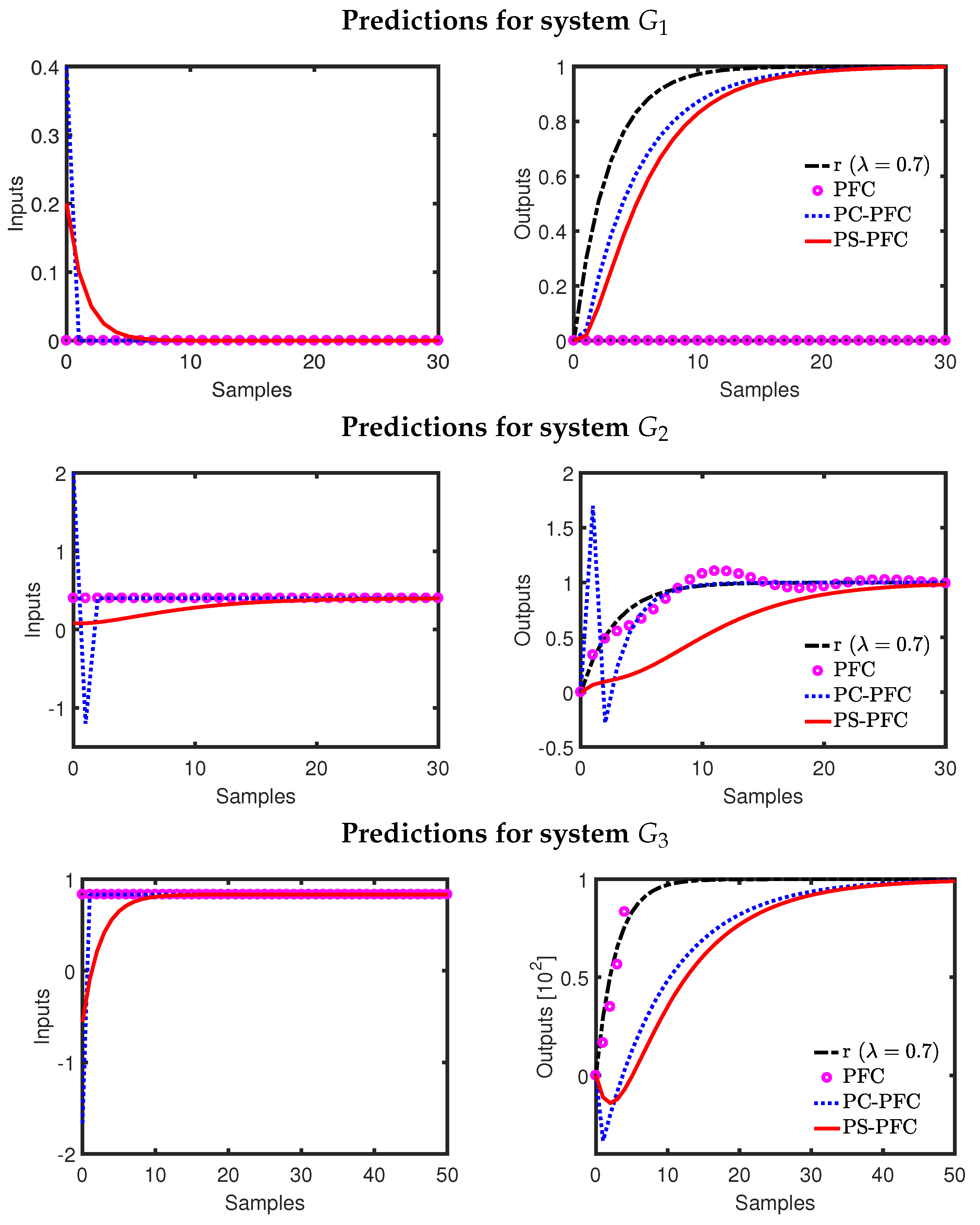
The prime purpose of shaping the future input dynamics is to eliminate the effect of unwanted poles in the future predictions. Nevertheless, it is also undesirable to have an overaggressive input activity, which may not be implementable in a real plant. To analyse this issue, the prediction behaviour of PFC, PC-PFC, and PS-PFC for processes $G_1$, $G_2$, and $G_3$ are plotted in Figure 2. From these results, it can be observed that:

• For an integrating process, such as $G_1$, the constant input prediction of PFC leads to a divergent output prediction, and thus, output constraints can only be satisfied if the input is selected to be zero! Hence, the PFC plots do not appear in this example, as the constraint handling forces a choice of $u_k=0,\forall k$.
• For $G_1$, the default input prediction (Equation (15)) for PC-PFC (blue-dotted line) is of dead-beat form and aggressive, whereas the input prediction (Equation (23)) for PS-PFC moves smoothly to the steady state and is less aggressive. There is no significant difference in the corresponding output predictions.
• For the underdamped system $G_2$, the output prediction from PFC includes a significant oscillation, which is undesirable and will also cause constraint handling to be conservative. The differences between PC-PFC and PS-PFC predictions are similar to those noted for $G_1$, that is, PS-PFC has a much smoother and less aggressive input prediction, albeit slow, and output prediction, due to the choice of $\alpha$. Of course, this difference means that the constraint handling for PS-PFC will be far more preferable and less conservative, in general. Conversely, since PC-PFC cancelled out two of their oscillatory open-loop poles, a sudden spike or aggressive damping is expected in the output response.
• For the unstable process $G_3$, a conventional PFC cannot be used because the divergent predictions will automatically violate constraints so that no feasible choice for $u_k$ will exist. Once again, it is seen that the predictions for PS-PFC are preferable to those from PC-PFC.

In summary, PS-PFC produces the best prediction behaviour because it ensures convergent predictions which will satisfy constraints with less aggressive input predictions, and thus less conservative constraint handling, than given by PC-PFC/PFC.

4.3. Tuning Efficacy and Closed-Loop Performance: The Unconstrained Case

First we give a brief discussion on PFC tuning for completeness. In general terms, a good practice guidance is to select the coincidence horizon in between 40% and 80% rise of the step input response to the steady-state value [13]: here, $G_1$ ($4\le n\le 9$), $G_2$ ($8\le n\le 15$), and $G_3$ ($11\le n\le 21$). Selecting a smaller horizon will lead to a more aggressive input, while larger horizons reduce the efficacy of $\lambda$ as a tuning parameter.

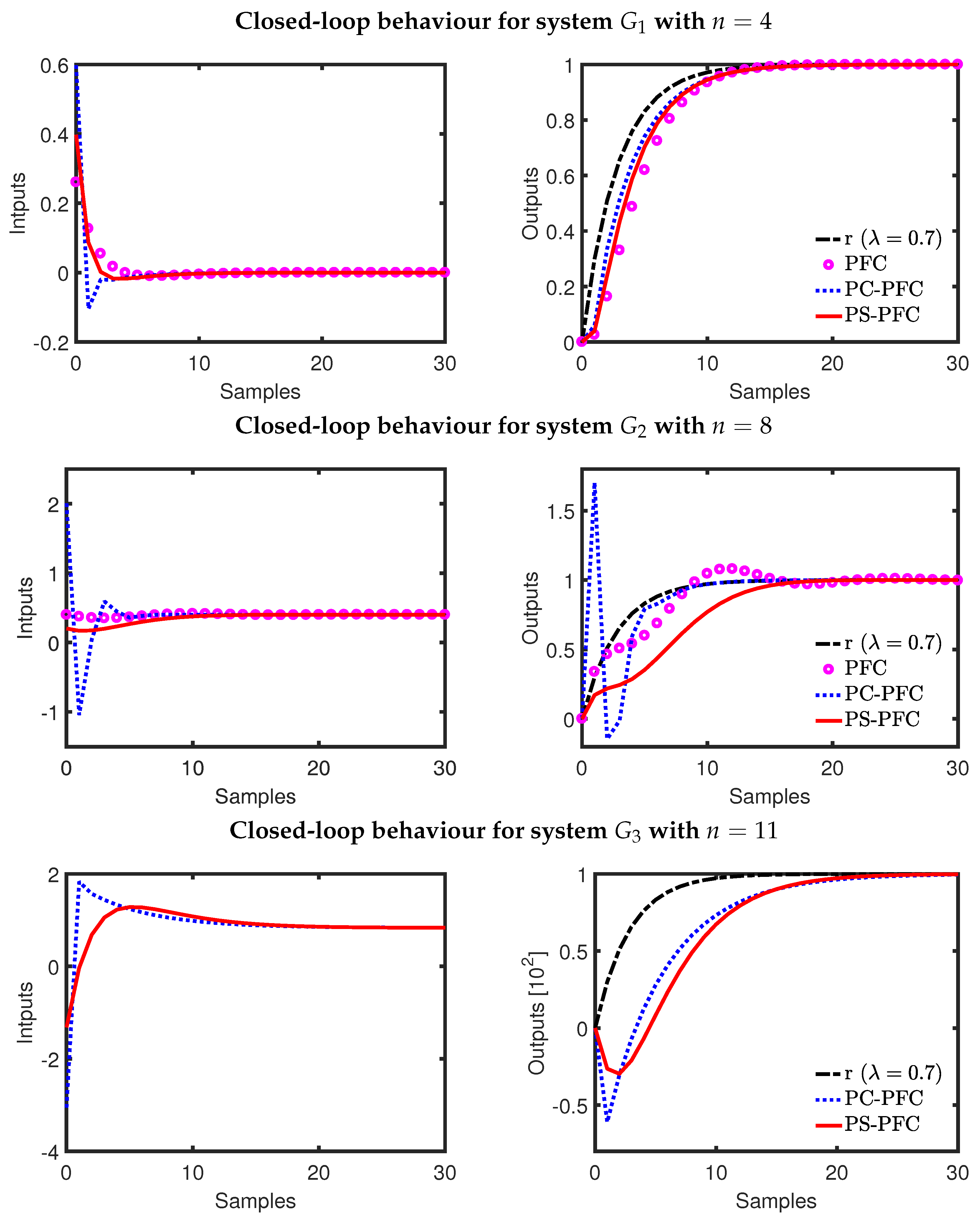
In general therefore, the main designer choice is the desired closed-loop pole; for simplicity of illustration, we take the desired pole to be $\lambda =0.7$. Figure 3 demonstrates the closed-loop performance of PFC, PC-PFC and PS-PFC on the three case study processes with these tunings. It is noted that:

• For all cases, PS-PFC (using a default choice of $\alpha$) gives the best trade-off between the rate of convergence and the aggressiveness of input activity compared to PFC and PC-PFC. Changes to $\alpha$ could offer a further tuning parameter for varying this trade-off.
• It is notable that PS-PFC gives similar or better output behaviour to PFC/PC-PFC while using a far smoother and less aggressive input trajectory.
• For processes $G_2,G_3$, the input and output behaviour of PC-PFC is extremely aggressive and would not be implementable in a real application.
• For process $G_3$, the conventional PFC cannot be stabilised with the given choice of n.

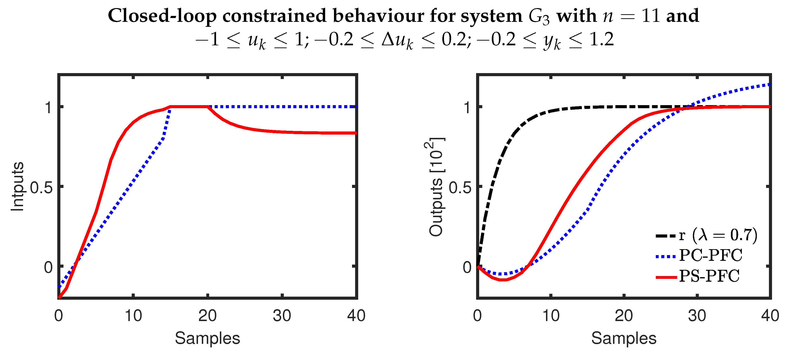
4.4. Constraint Handling

As noted in Section 4.2, for many dynamics a conventional PFC approach is infeasible or highly conservative because the output predictions inevitably violate constraints beyond a given horizon. Thus, conventional PFC can only be implemented by using short constraint horizons and thus with the loss of any recursive feasibility assurance; if it does work this is luck not good design and thus should be avoided. For the case studies here, conventional PFC could only be used safely with output constraints for $G_2$, although in that case we would expect some conservatism due to the oscillations in the output predictions.

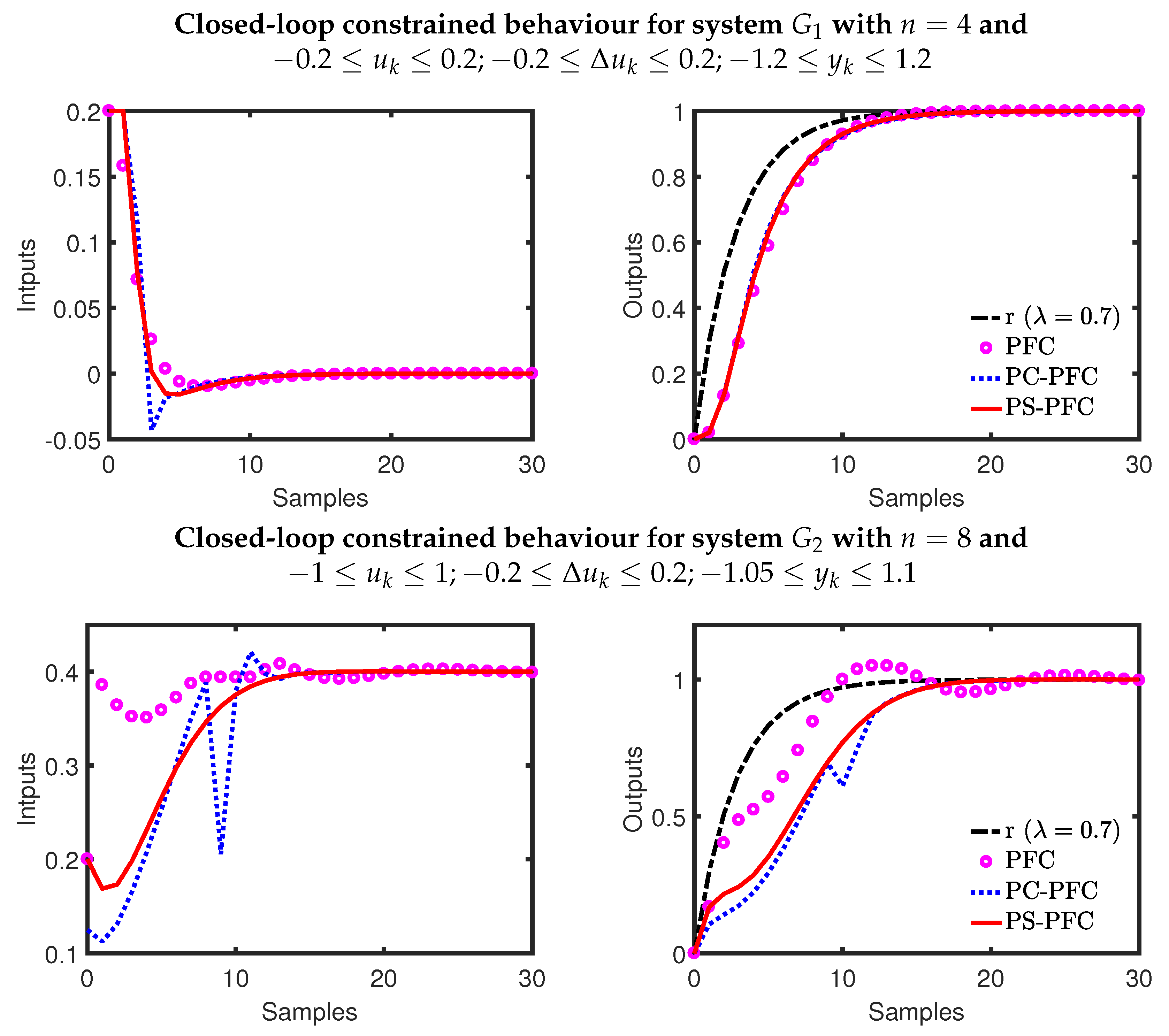
PC-PFC and PS-PFC pre-stabilise the output predictions and thus can be used safely and with a recursive feasibility assurance. Figure 4 compares the performance of PFC, PC-PFC, and PS-PFC when constraints are added to the process. Several observations can be noted:

• As expected, PS-PFC and PC-PFC satisfy constraints, retain recursive feasibility throughout and converge safely.
• For process $G_1$, the constrained performance of the controllers are almost the same, but PS-PFC provides a smoother input transition.
• For process $G_2$ it is clear that handling the under-damping will cause some challenges to any control law, but clearly PS-PFC provides the best responses.
• For process $G_3$, the inherent dead-beat input predictions deployed by PC-PFC mean the performance is poor and slow to converge whereas PS-PFC performs well.

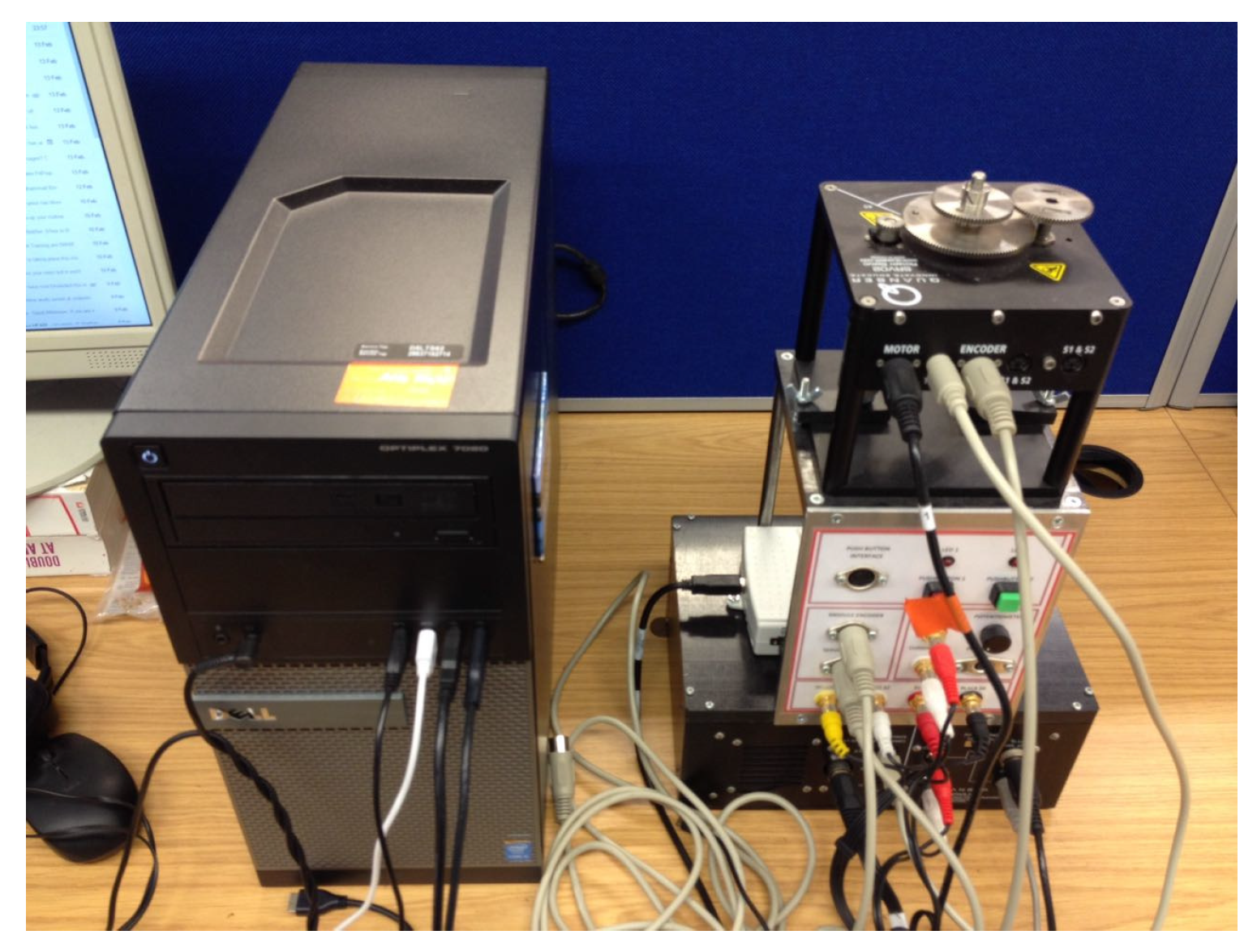
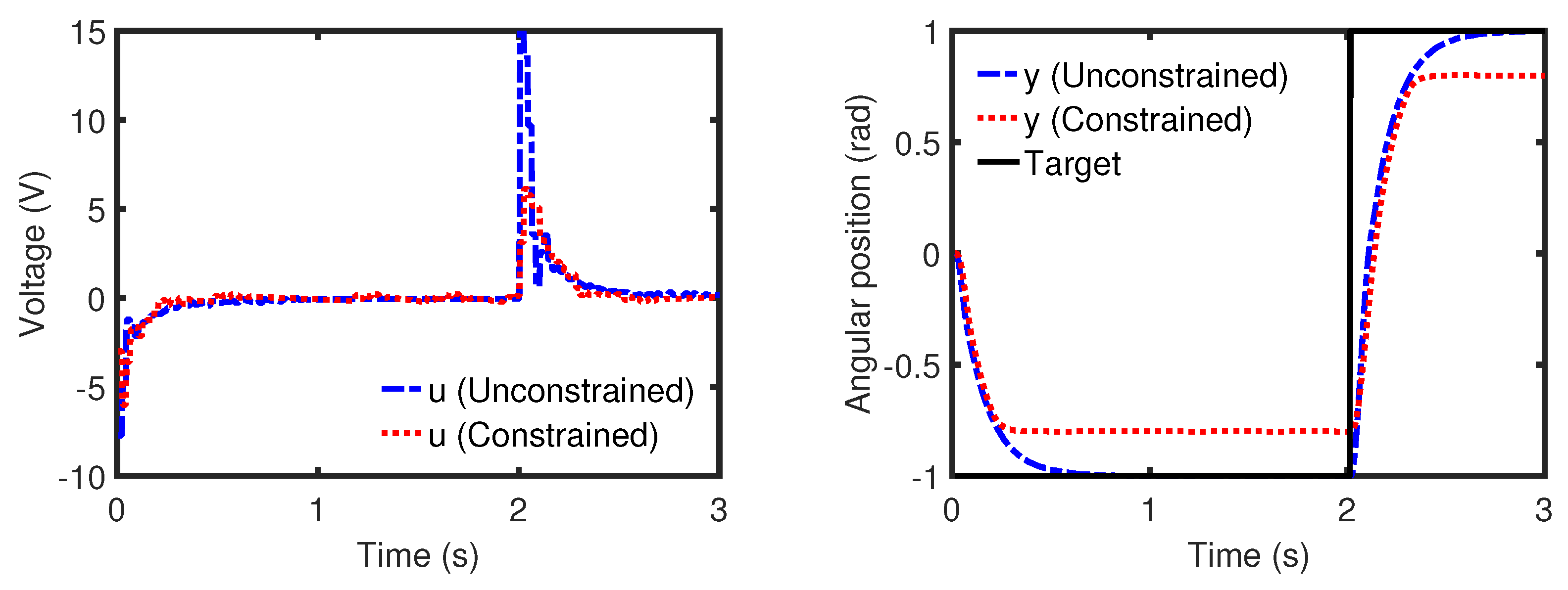
4.5. Application of PS-PFC on Laboratory Hardware

This section demonstrates the implementation of PS-PFC on laboratory hardware, that is, a Quanser SRV02 servo-based unit (Quanser, Markham, ON, Canada) (see Figure 5). This device is powered by a Quanser VoltPAQ-X1 amplifier and operates by National Instrument ELVIS II+ (National Instruments, Austin, TX, USA) multifunctional data acquisition via USB connection. The control objective is to track the servo position $\theta \left(t\right)$, measured in radians, by manipulating the supplied voltage $V\left(t\right)$. This servo will rotate counter-clockwise with positive supplied voltage and vice versa. A second-order model of (33) with an integrator is used to represent the system dynamics (refer to [29] for a more formal derivation) as:

$$\theta \left(t\right)=\frac{1.53}{s(0.254s+1)}V\left(s\right)$$

(33)

To implement the proposed control law, the continuous model (33) is discretised with sampling time $0.02s$ to obtain the discrete model of:

$$G_s=\frac{0.0095z^{-2}+0.0073z^{-1}}{1-1.45z^{-1}+0.45z^{-2}}$$

(34)

The plant is set to have a CLTR of $0.2s$ (which is equivalent to $\lambda =0.89$). Using a similar procedure to that in the previous section, the coincidence horizon is selected at $n=4$. Figure 6 demonstrates the unconstrained and constrained performances of PS-PFC in tracking the servo position. In the unconstrained case, the controller manages to track the target position with the desired convergence speed. As for the constrained case, all the implied input limits ($-8\le u_k\le 8$), rate limits ($-3\le \Delta u_k\le 3$), and output limits ($-0.8\le y_k\le 0.8$) are satisfied systematically without any conflict.

5. Conclusions

This paper proposes two potential simple modifications to a conventional PFC algorithm to improve the constraint handling properties for processes with challenging dynamics, such as integrating modes, underdamping, or unstable modes. Both proposals use relatively simple algebra—in effect, the solution of a small number of linear simultaneous equations—to parameterise the future input trajectories which lead to convergent and desirable output behaviours; this is done in terms of a component to deal with the current state (or initial condition) and a free component for control purposes. A core contribution is to show that using the proposed parameterisations allows a simple proof of recursive feasibility so that the constraint handling can be performed more safely and reliably.

A specific novelty of this paper is the proposed PS-PFC algorithm, which gives a pragmatic and simple proposal for deriving input and output prediction pairs which do not require aggressive inputs during transients; the more classical alternative approach of PC-PFC, in general, deploys very aggressive inputs in transients and thus cannot be used in practice. Simulation evidence on a variety of simulation case studies and hardware demonstrates that the proposed PS-PFC algorithm significantly outperforms both a conventional PFC approach and PC-PFC.

Although, as with all predictive control laws, both PC-PFC and PS-PFC are robust to some parameter uncertainty and disturbances, a detailed sensitivity analysis is an important next step. Also, it is of particular interest to compare these approaches with the alternative feedback formulations for PFC [6,15] by way of systematic design, nominal performance, constraint handling, and sensitivity.

References

- Khadir, M.; Ringwood, J. Stability issues for first order predictive functional controllers: Extension to handle higher order internal models. In Proceedings of the International Conference on Computer Systems and Information Technology, Algiers, Algeria, 19–21 July 2005; pp. 174–179. [Google Scholar]
- Richalet, J. Industrial applications of model based predictive control. Automatica 1993, 29, 1251–1274. [Google Scholar] [CrossRef]
- Haber, R.; Rossiter, J.A.; Zabet, K. An alternative for PID control: Predictive functional Control—A tutorial. In Proceedings of the 2016 American Control Conference (ACC), Boston, MA, USA, 6–8 July 2016; pp. 6935–6940. [Google Scholar]
- Clarke, D.W.; Mohtadi, C. Properties of generalized predictive control. Automatica 1989, 25, 859–875. [Google Scholar] [CrossRef]
- Haber, R.; Bars, R.; Schmitz, U. Predictive Control in Process Engineering: From the Basics to the Applications; Wiley-VCH: Weinheim, Germany, 2011. [Google Scholar]
- Richalet, J.; O’Donovan, D. Predictive Functional Control: Principles and Industrial Applications; Springer: London, UK, 2009. [Google Scholar]
- Rossiter, J.A. A priori stability results for PFC. Int. J. Control 2016, 90, 305–313. [Google Scholar] [CrossRef]
- Zabet, K.; Rossiter, J.A.; Haber, R.; Abdullah, M. Pole-placement predictive functional control for under-damped systems with real numbers algebra. ISA Trans. 2017, 71, 403–414. [Google Scholar] [CrossRef] [PubMed]
- Khadir, M.; Ringwood, J. Extension of first order predictive functional controllers to handle higher order internal models. Int. J. Appl. Math. Comput. Sci. 2008, 18, 229–239. [Google Scholar] [CrossRef]
- Rossiter, J.A.; Haber, R.; Zabet, K. Pole-placement predictive functional control for over-damped systems with real poles. ISA Trans. 2016, 61, 229–239. [Google Scholar] [CrossRef] [PubMed]
- Abdullah, M.; Rossiter, J.A. Utilising Laguerre function in predictive functional control to ensure prediction consistency. In Proceedings of the 2016 UKACC 11th International Conference on Control (CONTROL), Belfast, UK, 31 August–2 September 2016. [Google Scholar]
- Abdullah, M.; Rossiter, J.A.; Haber, R. Development of constrained predictive functional control using Laguerre function based prediction. IFAC-PapersOnLine 2017, 50, 10705–10710. [Google Scholar] [CrossRef]
- Rossiter, J.A.; Haber, R. The effect of coincidence horizon on predictive functional control. Processes 2015, 3, 25–45. [Google Scholar] [CrossRef]
- Richalet, J.; Rault, A.; Testud, J.; Papon, J. Model predictive heuristic control: Applications to industrial processes. Automatica 1987, 14, 413–428. [Google Scholar] [CrossRef]
- Zhang, Z.; Rossiter, J.A.; Xie, L.; Su, H. Predictive Functional Control for Integral Systems; PSE: Bellevue, WD, USA, 2018. (In Chinese) [Google Scholar]
- Rossiter, J.A. Input shaping for pfc: How and why? J. Control Decis. 2015, 3, 105–118. [Google Scholar] [CrossRef]
- Mosca, E.; Zhang, J. Stable redesign of predictive control. Automatica 1992, 28, 1229–1233. [Google Scholar] [CrossRef]
- Rossiter, J.A. Predictive functional control: More than one way to pre stabilise. In Proceedings of the 15th Triennial World Congress, Barcelona, Spain, 21–26 July 2002; pp. 289–294. [Google Scholar]
- Rawlings, J.; Muske, K. The stability of constrained receding horizon control. IEEE Trans. Autom. Control 1993, 38, 1512–1516. [Google Scholar] [CrossRef]
- Richalet, J.; O’Donovan, D. Elementary predictive functional control: A tutorial. In Proceedings of the 2011 International Symposium on Advanced Control of Industrial Processes (ADCONIP), Hangzhou, China, 23–26 May 2011; pp. 306–313. [Google Scholar]
- Rossiter, J.A. A First Course in Predictive Control, 2nd ed.; CRC Press: London, UK, 2018. [Google Scholar]
- Nise, N.S. Control System Engineering; John Wiley & Sons, Inc.: New York, NY, USA, 2011. [Google Scholar]
- Gilbert, E.; Tan, K. Linear systems with state and control constraints: The theory and application of maximal admissible sets. IEEE Trans. Autom. Control 1991, 36, 1008–1020. [Google Scholar] [CrossRef]
- Fiani, P.; Richalet, J. Handling input and state constraints in predictive functional control. In Proceedings of the 30th IEEE Conference on Decision and Control, Brighton, UK, 11–13 December 1991; pp. 985–990. [Google Scholar]
- Rossiter, J.A.; Kouvaritakis, B. Numerical robustness and efficiency of generalised predictive control algorithms with guaranted stability. IEE Proc. D 1994, 141, 154–162. [Google Scholar]
- Scokaert, P.O.; Rawlings, J.B. Constrained linear quadratic regulation. IEEE Trans. Autom. Control 1998, 43, 1163–1169. [Google Scholar] [CrossRef] [Green Version]
- Zhuo, W.; Shichao, W.; Yanyan, J. Simulation of control of water level in boiler drum. In Proceedings of the World Automation Congress 2012, Puerto Vallarta, Mexico, 24–28 June 2012. [Google Scholar]
- Kendi, T.A.; Doyle, F.J., III. Nonlinear control of a fluidized bed reactor using approximate feedback linearization. Ind. Eng. Chem. Res. 1996, 35, 746–757. [Google Scholar] [CrossRef]
- Apkarian, J.; Lévis, M.; Gurocak, H. Instructor Workbook: SVR02 Based Unit Experiment for LabVIEW Users; Quanser Inc.: Markham, ON, Canada, 2012. [Google Scholar]
Figure 1.
Comparison of flow diagrams for predictive functional control (PFC), model predictive control (MPC), and proportional integral derivative (PID).
Figure 2.
Input and output predictions with PFC, PC-PFC, and PS-PFC for processes .
Figure 3.
Closed-loop input and output behaviour of PC-PFC and PS-PFC for processes .
Figure 4.
Constrained input and output behaviour of PFC, Pole Cancellation PFC (PC-PFC), and Pole Shaping PFC (PS-PFC) for processes .
Figure 5.
Quanser SRV02 servo based unit.
Figure 6.
Unconstrained and constrained performance of PS-PFC for process .
© 2018 by the authors. Licensee MDPI, Basel, Switzerland. This article is an open access article distributed under the terms and conditions of the Creative Commons Attribution (CC BY) license (http://creativecommons.org/licenses/by/4.0/).
Share and Cite
MDPI and ACS Style
Abdullah, M.; Rossiter, J.A. Input Shaping Predictive Functional Control for Different Types of Challenging Dynamics Processes. Processes 2018, 6, 118. https://doi.org/10.3390/pr6080118
AMA Style
Abdullah M, Rossiter JA. Input Shaping Predictive Functional Control for Different Types of Challenging Dynamics Processes. Processes. 2018; 6(8):118. https://doi.org/10.3390/pr6080118
Chicago/Turabian StyleAbdullah, Muhammad, and John Anthony Rossiter. 2018. "Input Shaping Predictive Functional Control for Different Types of Challenging Dynamics Processes" Processes 6, no. 8: 118. https://doi.org/10.3390/pr6080118
Note that from the first issue of 2016, this journal uses article numbers instead of page numbers. See further details here.