Dynamic Sequence Specific Constraint-Based Modeling of Cell-Free Protein Synthesis

Abstract

Cell-free protein expression has emerged as an important approach in systems and synthetic biology, and a promising technology for personalized point of care medicine. Cell-free systems derived from crude whole cell extracts have shown remarkable utility as a protein synthesis technology. However, if cell-free platforms for on-demand biomanufacturing are to become a reality, the performance limits of these systems must be defined and optimized. Toward this goal, we modeled E. coli cell-free protein expression using a sequence specific dynamic constraint-based approach in which metabolite measurements were directly incorporated into the flux estimation problem. A cell-free metabolic network was constructed by removing growth associated reactions from the iAF1260 reconstruction of K-12 MG1655 E. coli. Sequence specific descriptions of transcription and translation processes were then added to this metabolic network to describe protein production. A linear programming problem was then solved over short time intervals to estimate metabolic fluxes through the augmented cell-free network, subject to material balances, time rate of change and metabolite measurement constraints. The approach captured the biphasic cell-free production of a model protein, chloramphenicol acetyltransferase. Flux variability analysis suggested that cell-free metabolism was potentially robust; for example, the rate of protein production could be met by flux through the glycolytic, pentose phosphate, or the Entner-Doudoroff pathways. Variation of the metabolite constraints revealed central carbon metabolites, specifically upper glycolysis, tricarboxylic acid (TCA) cycle, and pentose phosphate, to be the most effective at training a predictive model, while energy and amino acid measurements were less effective. Irrespective of the measurement set, the metabolic fluxes (for the most part) remained unidentifiable. These findings suggested dynamic constraint-based modeling could aid in the design of cell-free protein expression experiments for metabolite prediction, but the flux estimation problem remains challenging. Furthermore, while we modeled the cell-free production of only a single protein in this study, the sequence specific dynamic constraint-based modeling approach presented here could be extended to multi-protein synthetic circuits, RNA circuits or even small molecule production.

1. Introduction

Cell-free protein expression has become a widely used research tool in systems and synthetic biology, and a promising technology for personalized point of use biotechnology [1]. Cell-free systems offer many advantages for the study, manipulation and modeling of metabolism compared to in vivo processes. Central amongst these is direct access to metabolites and the biosynthetic machinery, without the interference of a cell wall or the complications associated with cell growth. This allows us to interrogate (and potentially manipulate) the chemical microenvironment while the biosynthetic machinery is operating, potentially at a fine time resolution. Cell-free protein synthesis (CFPS) systems are arguably the most prominent examples of cell-free systems used today [2]. However, CFPS in crude E. coli extracts has been used previously to explore fundamental biological questions. For example, Matthaei and Nirenberg used E. coli cell-free extracts to decipher the genetic code [3,4]. Later, Spirin and coworkers continuously exchanged reactants and products in a CFPS reaction, which improved protein production. However, while these extracts could run for up to tens of hours, they could only synthesize a single product and were likely energy limited [5]. More recently, energy and cofactor regeneration in CFPS has been significantly improved; for example, ATP can be regenerated using substrate level phosphorylation [6] or even oxidative phosphorylation [2]. Today, cell-free systems are used in a variety of applications ranging from therapeutic protein production [7] to synthetic biology [1,8]. There are also several CFPS technology platforms, such as the PANOx-SP (PEP, Amino Acids, NAD, Oxalic Acid, Spermidine, and Putrescine) and Cytomin platforms developed by Swartz and coworkers [2,9], and the transcription and translation (TX-TL) platform of Noireaux [10]. Taken together, CFPS is a promising technology for protein production. However, if CFPS is to become a mainstream technology for applications such as point of care biomanufacturing, we must first understand the performance limits of these systems, and eventually optimize their yield and productivity. Toward this unmet need, we have developed a dynamic constraint-based modeling that can be used to interrogate cell-free systems.

Genome scale stoichiometric reconstructions of microbial metabolism popularized by static, constraint-based modeling techniques such as flux balance analysis (FBA) have become standard tools [11]. Since the first genome scale stoichiometric model of E. coli, developed by Edwards and Palsson [12], well over 100 organisms, including industrially important prokaryotes such as E. coli [13] or B. subtilis [14], are now available [15]. Stoichiometric models rely on a pseudo-steady-state assumption to reduce unidentifiable genome-scale kinetic models to an underdetermined linear algebraic system, which can be solved efficiently even for large systems using linear programming. Traditionally, stoichiometric models have also neglected explicit descriptions of metabolic regulation and control mechanisms, instead opting to describe the choice of pathways by prescribing an objective function on metabolism. Interestingly, similar to early cybernetic models, the most common metabolic objective function has been the optimization of biomass formation [16], although other metabolic objectives have also been estimated [17]. Recent advances in constraint-based modeling have overcome the early shortcomings of the platform, including describing metabolic regulation and control [18] and incorporating genome sequence into the model [19,20]. Dynamic constraint-based methods have also been developed in which the metabolic flux is computed over short-time intervals subject to time-varying constraints [21]. These methods are common, have been used in varied applications, [22,23,24,25], and there are open source packages to support this class of calculation [26,27,28]. Thus, constraint-based approaches, and their dynamic extensions, have proven useful in the discovery of metabolic engineering strategies and represent the state of the art in metabolic modeling [29,30]. However, while constraint-based tools have been used extensively to analyze whole cells systems, they have not yet been widely applied to study cell-free reactions.

In this study, we constructed a dynamic constraint-based model of cell-free protein expression. This approach avoids the pseudo-steady-state assumption found in traditional constraint-based approaches, which allowed for the direct integration of dynamic metabolite measurements into the flux estimation problem, along with the accumulation or depletion of network metabolites. We adapted the sequence specific constraint-based model of Vilkhovoy and coworkers [31] into a dynamic constraint-based model of cell-free E. coli metabolism and protein production, and leveraged the kinetic model of Horvath and coworkers [32] to provide synthetic data to inform metabolite constraints. CFPS synthesis is often (but not always) conducted in small scale batch reactors. Thus, the concentration of the components of the reaction mixture, and the associated rates of the metabolic processes in the reaction are not always constant. The Vilkhovoy et al. study considered only the first hour of the CFPS reaction producing the model protein, chloramphenicol acetyltransferase (CAT). During this initial phase, the metabolic rates were approximately constant and a classical sequence specific flux balance analysis approach was sufficient to describe protein synthesis [31]. However, after this initial phase, there was a significant shift in productivity following the exhaustion of glucose (which occurred at approximately 1.5 h). Horvath and coworkers developed a fully kinetic model that described the complete three hour reaction time course, including the shift in productivity following glucose exhaustion [32]. While this model described the CFPS dynamics, and the decrease in productivity following the exhaustion of glucose, the identification of the model from 37 measured metabolite trajectories was difficult. Thus, there was an unmet need for a tool that could describe the dynamics of a CFPS reaction, without the burden of identifying a full kinetic model. Toward this need, we developed a dynamic constraint-based modeling approach for CFPS reactions which directly incorporated metabolite measurements (as constraints) into the flux calculation. The dynamic constraint-based model satisfied time-dependent metabolite constraints, while predicting the concentration of the CAT protein and unconstrained metabolite concentrations. Model interrogation suggested the most important metabolite constraint was glucose, as excluding glucose yielded the greatest metabolite prediction error, and the greatest uncertainty in the estimated metabolic flux. Furthermore, we evaluated metabolite constraint sets with one more and one fewer metabolites than the base case (the 37 measured metabolites) to explore the impact of measurement selection on model performance. The single addition of metabolites yielded no significant improvement in the predictive power, while the single exclusion suggested glucose to be the most important measured metabolite in the base case. Next, we selected measurement species based on the results of singular value decomposition on the stoichiometric matrix. The top 36 species from the singular value decomposition (SVD) analysis with the addition of glucose improved the predictive power and reduced flux uncertainty compared with the base case. Finally, we developed a heuristic optimization approach to estimate the optimal list of metabolite measurements. This approach significantly improved metabolite prediction compared to the base case. However, both the base measurement set and the heuristically optimized experimental design poorly characterized flux uncertainty. Taken together, this suggested that dynamic constraint-based modeling can aid in experimental design and measurement selection for metabolite prediction, but the flux estimation problem remains challenging. Furthermore, while we modeled the cell-free production of only a single protein in this study, the sequence specific dynamic constraint-based modeling approach presented here could be extended to multi-protein synthetic circuits, RNA circuits [33] or even small molecule production.

2. Results

2.1. Cell-Free E. coli Metabolic Network

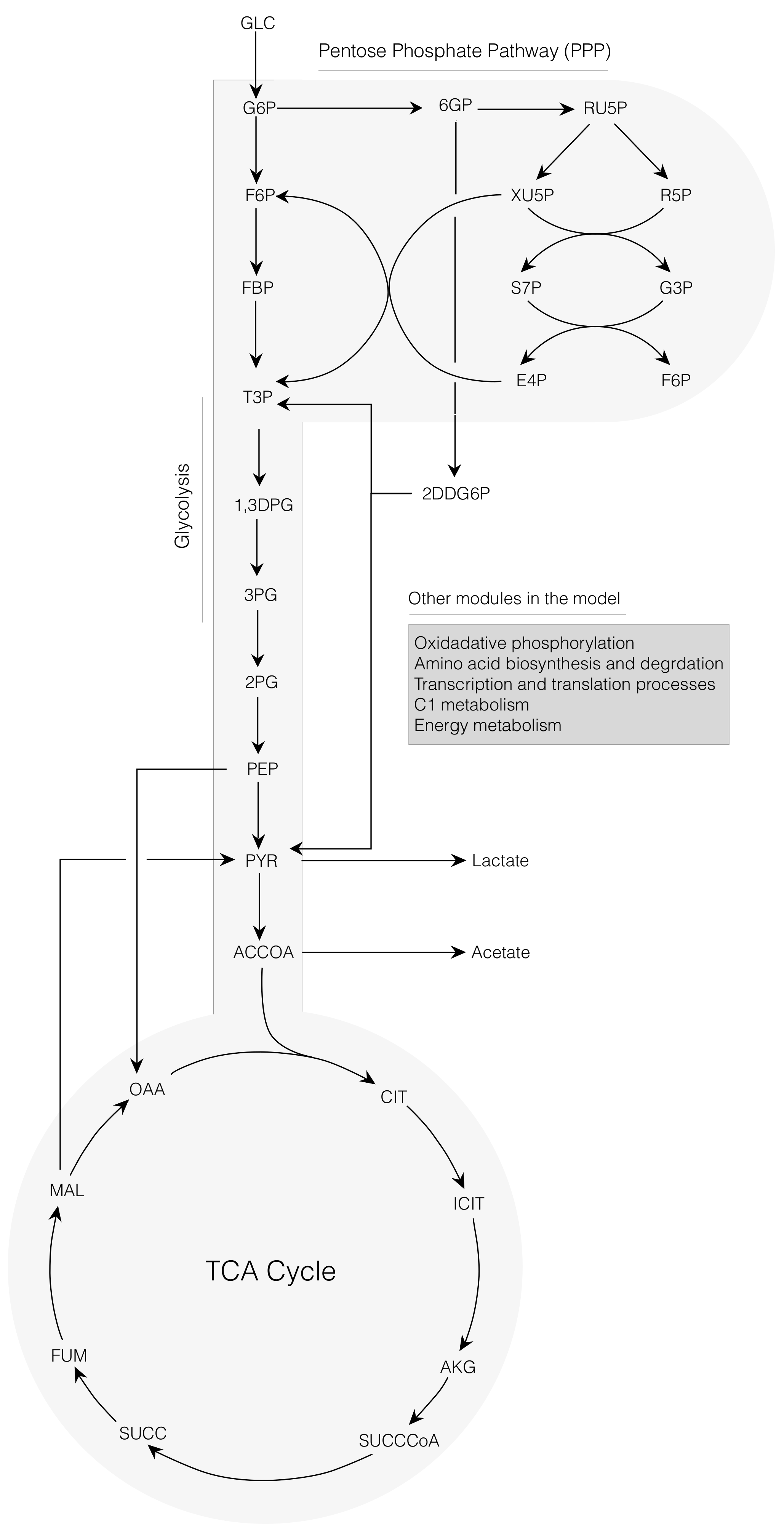
We constructed the cell-free stoichiometric network by removing growth associated reactions from the iAF1260 reconstruction of K-12 MG1655 E. coli [13], and removing reactions not present in the cell-free system (see Materials and Methods). We then added the transcription and translation template reactions of Allen and Palsson for the CAT protein [19]. Thus, our stoichiometric network described the material and energetic demands for transcription and translation at sequence specific level. The metabolic network consisted of 264 reactions and 146 species; a schematic of the central carbon metabolism is shown in Figure 1. The network described the major carbon and energy pathways and amino acid biosynthesis and degradation pathways. Lastly, we removed genes from the network that were knocked out in the E. coli host strain used to make the cell-free extract (A19 $\mathrm{\Delta }$tonA $\mathsf{\Delta }$tnaA $\Delta$speA $\Delta$endA $\Delta$sdaA $\Delta$sdaB $\Delta$gshA); see Jewett et al. for further details of the host strain and the cell-free extract preparation [34]. Using this network, we simulated time-dependent cell-free production of the model protein CAT. We used dynamic modified flux balance analysis, a stoichiometric modeling technique that does not make the pseudo steady state assumption and allows the accumulation and depletion of metabolite species. Horvath and coworkers predicted time-dependent cell-free production of CAT using a fully kinetic model trained against an experimental dataset of 37 metabolites, including the substrate glucose, the protein product CAT, organic acids, amino acids, and energy species [32]. This model was used to generate the metabolite constraints used in this study. Transcription and translation rates were subject to resource constraints encoded by the metabolic network, and transcription and translation model parameters were largely derived from literature (

Table 1. Reference values for transcription, translation, and mRNA degradation from literature. Transcription rate calculated from elongation rate, mRNA length, and promoter activity level. Translation rate calculated from elongation rate, protein length, and polysome amplification constant. The mRNA degradation rate calculated from a characteristic mRNA half-life. CAT: chloramphenicol acetyltransferase.

Description	Parameter	Value	Units	Reference
T7 RNA polymerase concentration	$R_T$	1.0	$\mathsf{\mu }$M
Ribosome concentration	$R_X$	2	$\mathsf{\mu }$M	[10]
CAT mRNA length	$l_G$	660	nt	[36]
CAT protein length	$l_P$	219	aa	[36]
Transcription saturation coefficient	$K_T$	100	nM	estimated
Transcription elongation rate	${\dot{v}}_T$	25	nt/s	[10]
Translation saturation coefficient	$K_X$	45	$\mathsf{\mu }$M	estimated
Translation elongation rate	${\dot{v}}_X$	1.5	aa/s	[10]
T7 Promoter activity level	u	0.9		estimated
Transcription rate	$k_{cat}^T=\left({\displaystyle \frac{{\dot{v}}_T}{l_G}}\right)u$	123	h−1	calculated
Polysome amplification constant	$K_P$	10		estimated
Translation rate	$k_{cat}^X=\left({\displaystyle \frac{{\dot{v}}_X}{l_P}}\right)K_P$	247	h−1	calculated
mRNA degradation time	$t_{1/2}$	8	min	BNID 106253
mRNA degradation rate	$k_{deg}={\displaystyle \frac{ln\left(2\right)}{t_{1/2}}}$	5.2	h−1	calculated

). In this study, we did not explicitly consider protein folding. However, the addition of chaperone or other protein maturation steps could easily be accommodated within the approach by updating the template reactions (see Palsson and coworkers [20]). The cell-free metabolic network and all model code and parameters can be downloaded under an MIT software license from the Varnerlab website [35].

2.2. Dynamic Constrained Simulation of cell-free Protein Synthesis

Cell-free synthesis of the CAT protein showed two production phases, an initial fast production phase before glucose exhaustion (at approximately 1.5 h) and a slow production phase following glucose exhaustion. The metabolite profile varied significantly between these phases; for example, pyruvate and lactate were produced during the first phase but consumed during the second. Thus, a static pseudo steady state flux balance approach was not possible for this system. However, a central advantage of cell-free systems is direct access to metabolite measurements, and the biosynthetic machinery during production. If we could directly integrate dynamic metabolite and protein concentration measurements into the flux estimation problem, we could potentially get a better estimate of the flux distribution. Toward this question, we developed a dynamic modeling approach in which metabolic fluxes were estimated so that all metabolites were non-negative and the simulated metabolites were constrained to lie within a bounded range of the measured value. Using this technique, we simulated the cell-free production of CAT subject to dynamic metabolite measurements.

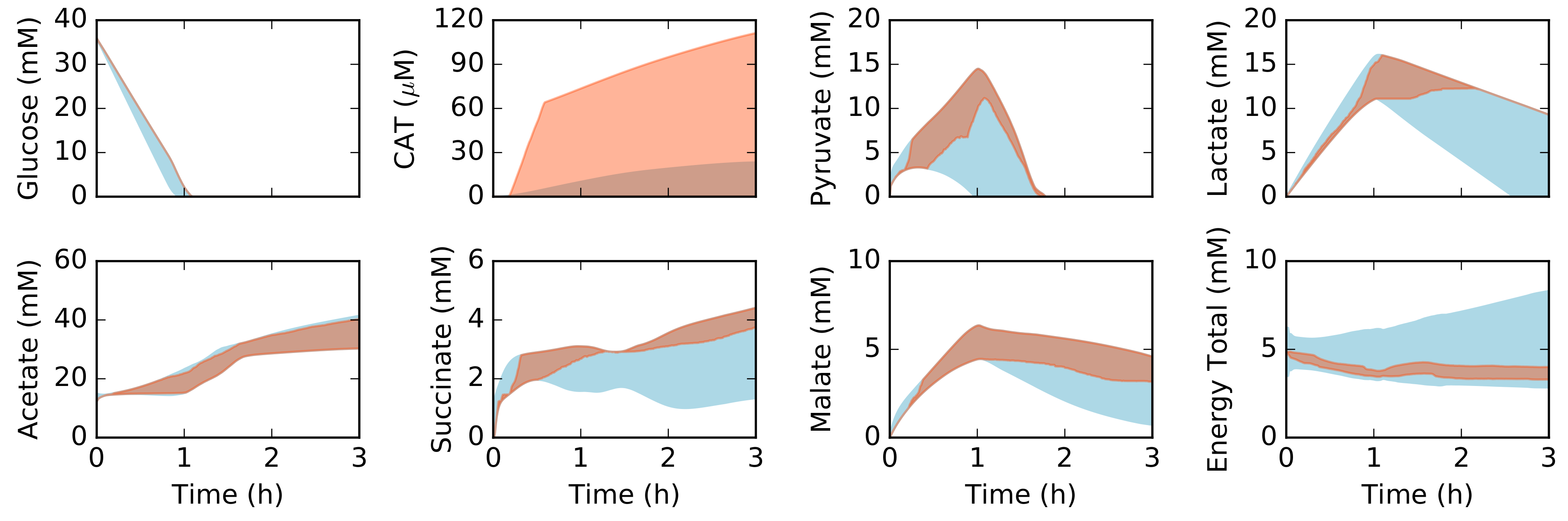
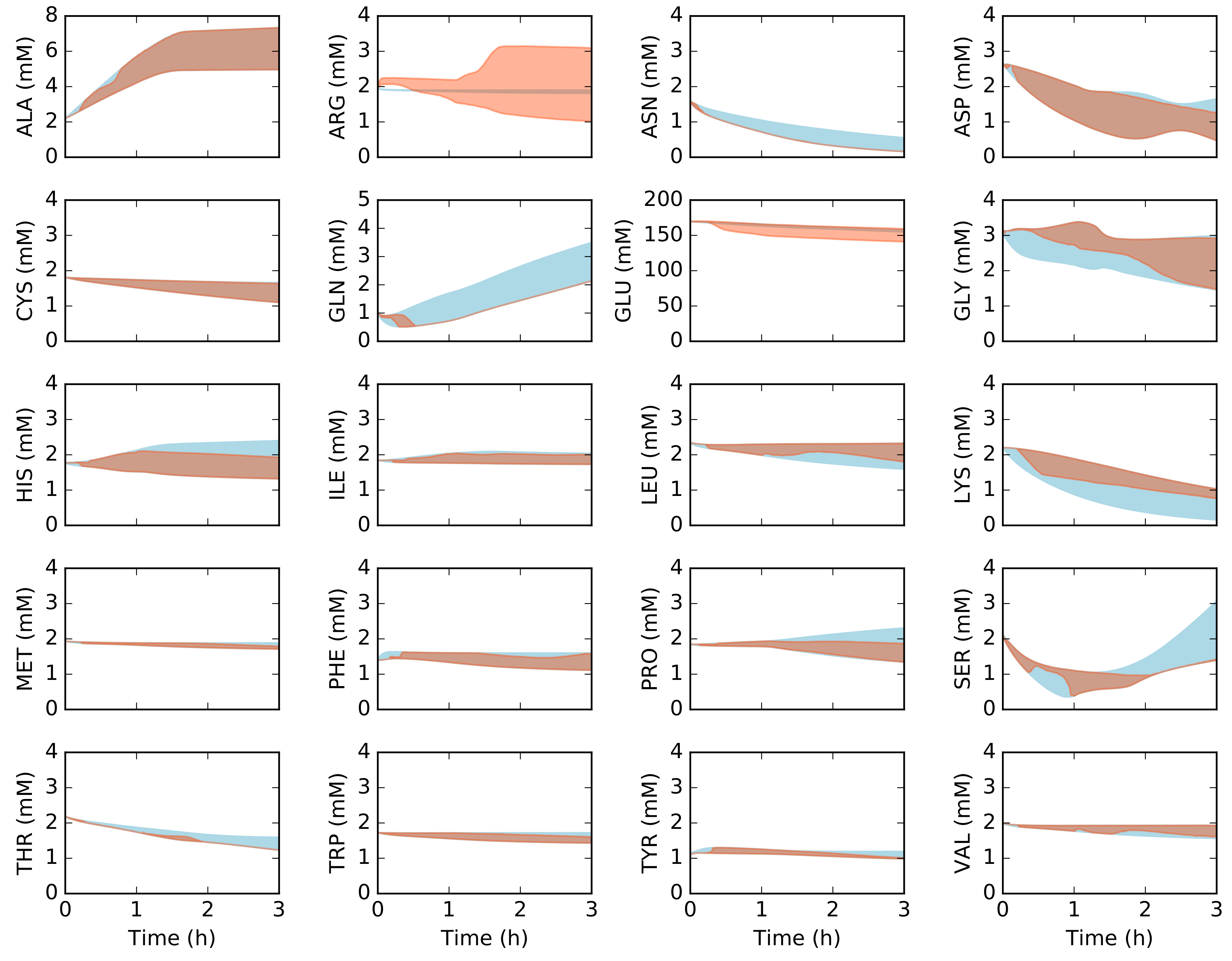
We explored the influence of uncertainty in the transcription (TX) and translation parameters (TL) by sampling different values for the abundance and elongation rates of RNA polymerases and ribosomes, the polysome amplification constant, the mRNA degradation rate and other kinetic parameters appearing in the transcription and translation bounds. The base values for the TX/TL parameters are given in Table 1, and the uniform sampling procedure is described in the Materials and Methods. Central carbon metabolites (Figure 2), amino acids (Figure 3), and energy species (Figure 4) in the synthetic measurement set were captured, within experimental error, by an ensemble of dynamic constraint-based simulations. The synthetic metabolite constraints (blue regions) shown in each of the simulation figures was derived from the kinetic model of Horvath et al. [32], which was trained on experimental measurement of the 37 metabolites shown in Figure 2, Figure 3 and Figure 4. Thus, the metabolite constraints used in this study were calculated based upon the kinetic model, which shows high fidelity with the experimental measurements. The flux estimation problem converged in greater than 99% of the simulation time intervals, given these metabolite constraints. This suggested there were not gross measurement errors in the measurement constraints, as the stoichiometric constraints were satisfied. Moreover, it suggested the error introduced by the time discretization scheme did not lead to inconsistent metabolite estimates. The ensemble of models captured the time evolution of protein biosynthesis, and the consumption and production of organic acid, amino acid and energy species. Arginine and glutamate were excluded from the constraint set, but were still largely captured by the ensemble of dynamic constraint-based models, although with wide variance than the synthetic measurement set. During the first hour, glucose was consumed as the primary carbon source for ATP, amino acids, and protein synthesis. After glucose was depleted, lactate and pyruvate were consumed as alternate substrates for energy production and CAT synthesis. Taken together, we captured the 37 metabolite measurements in the base synthetic data set, and captured the biphasic behavior of CAT production, although we significantly over-predicted the translation rate for some elements of the ensemble. This suggested that there was excess capacity in the metabolic network, which could be used to enhance protein production.

We quantified the uncertainty in the estimated metabolic flux distribution, given constrained CAT production using flux variability analysis (FVA) for the base synthetic data across the three hours of measurement (

Table 2. Flux uncertainty calculated using flux variability analysis for the base synthetic dataset during the first production phase (0 h to 1.5 h), normalized to the glucose consumption rate.

Enzyme/Pathway	Reaction	Uncertainty
RNA polymerase	Translation	<0.01
RNA polymerase	Translation initiation	<0.01
tRNA charging of alanine	tRNA charging (ALA)	<0.01
tRNA charging of cysteine	tRNA charging (CYS)	<0.01
tRNA charging of aspartate	tRNA charging (ASP)	<0.01
tRNA charging of histidine	tRNA charging (HIS)	<0.01
tRNA charging of serine	tRNA charging (SER)	<0.01
tRNA charging of tyrosine	tRNA charging (TYR)	<0.01
tRNA charging of phenylalanine	tRNA charging (PHE)	<0.01
tRNA charging of arginine	tRNA charging (ARG)	<0.01
tRNA charging of glutamate	tRNA charging (GLU)	<0.01
mRNA degradation	mRNA degradation	<0.01
tRNA charging of tryptophan	tRNA charging (TRP)	<0.01
tRNA charging of proline	tRNA charging (PRO)	<0.01
tRNA charging of asparagine	tRNA charging (ASN)	<0.01
tRNA charging of isoleucine	tRNA charging (ILE)	<0.01
tRNA charging of glycine	tRNA charging (GLY)	<0.01
tRNA charging of glutamine	tRNA charging (GLN)	<0.01
tRNA charging of lysine	tRNA charging (LYS)	<0.01
tRNA charging of threonine	tRNA charging (THR)	<0.01
tRNA charging of valine	tRNA charging (VAL)	<0.01
tRNA charging of methionine	tRNA charging (MET)	<0.01
tRNA charging of leucine	tRNA charging (LEU)	<0.01
Step 6 of AMP synthesis	R_A_syn_6	<0.01
Orotate synthase 1	R_or_syn_1	<0.01
Metionine biosynthesis	R_met	0.01
Valine biosynthesis	R_val	0.01
Leucine biosynthesis	R_leu	0.01
Aldhyde-alcohol dehydrogenase	R_adhE_net	0.01
Malate dehydrogenase	R_mdh_net	0.01
Glycine biosynthesis	R_gly_deg	0.02
Threonine degradation 2	R_thr_deg2	0.02
Acetate kinase	R_ackA_net	0.02
Alanine biosynthesis	R_alaAC_net	0.02
Isoleucine biosynthesis	R_ile	0.03
Tyrosine biosynthesis	R_tyr	0.03
Histidine biosynthesis	R_his	0.03
Methylglyoxal degradation	R_mglx_deg	0.03
Transaldolase	R_talAB_net	0.04
Glycine cleavage system	R_gly_fol_net	0.04
Ribulose-phosphate 3-epimerase	R_rpe_net	0.04
Phosphate acetyltransferase	R_pta_net	0.04
Phosphoglycerate kinase	R_pgk_net	0.05
Glyceraldehyde-3-phosphate dehydrogenase	R_gapA_net	0.05
Fructose 1,6-bisphosphate aldolase	R_fbaA_net	0.05
Enolase	R_eno_net	0.05
Phenylalanine biosynthesis	R_phe	0.05
Transketolase 2	R_tkt2_net	0.06
Fumarate hydratase	R_fum_net	0.06
Transketolase 1	R_tkt1_net	0.07
Orotate synthase 2	R_or_syn_2	0.07
Phosphoglycerate mutase	R_gpm_net	0.08
Ribose-5-phosphate isomerase	R_rpi_net	0.09
CTP synthetase 1	R_ctp_1	0.09
CTP synthetase 2	R_ctp_2	0.09
Triosephosphate isomerase	R_tpiA_net	0.1
Step 7 of AMP synthesis	R_A_syn_7	0.15
Step 12 of AMP synthesis	R_A_syn_12	0.17
Lactate dehydrogenase	R_ldh_net	0.17
Step 5 of AMP synthesis	R_A_syn_5	0.2
Methylenetetrahydrofolate reductase	R_mthfr2a	0.2
Glucose-6-phosphate dehydrogenase	R_zwf_net	0.21
Methylenetetrahydrofolate dehydrogenase	R_mthfd_net	0.21
UMP synthesis	R_ump_syn	0.22
OMP synthesis	R_omp_syn	0.22
Lysine degradation	R_lys_deg	0.23
Lysine biosynthesis	R_lys	0.23
Isocitrate dehydrogenase	R_icd_net	0.23
Threonine degradation 3	R_thr_deg3	0.24
Step 8 of AMP synthesis	R_A_syn_8	0.26
Tryptophan degradation	R_trp_deg	0.27
Methylenetetrahydrofolate dehydrogenase	R_mthfc_net	0.28
Tryptophan biosynthesis	R_trp	0.28
Aconitase	R_acn_net	0.33
Phosphoglucose isomerase	R_pgi_net	0.33
Step e of folate synthesis	R_fol_e	0.34
Step 4 of AMP synthesis	R_A_syn_4	0.4
GMP synthetase	R_gmp_syn	0.44
Step 9 of AMP synthesis	R_A_syn_9	0.48
XMP synthase	R_xmp_syn	0.53
Step 3 of AMP synthesis	R_A_syn_3	0.6
Step 10 of AMP synthesis	R_A_syn_10	0.63
Step 2b of folate synthesis	R_fol_2b	0.63
Glutamate dehydrogenase	R_gdhA_net	0.71
Step 3 of folate synthesis	R_fol_3	0.74
Step 4 of folate synthesis	R_fol_4	0.79
Pyruvate formate lyase	R_pflAB	0.8
Step 2 of AMP synthesis	R_A_syn_2	0.81
Step 2a of folate synthesis	R_fol_2a	0.81
Step 1 of folate synthesis	R_fol_1	0.99
Glucokinase	R_glk_atp	1
Step 1 of AMP synthesis	R_A_syn_1	1
Arginine degradation	R_arg_deg	1.23
Glycine biosynthesis	R_glyA	1.33
Phosphoribosylpyrophosphate synthase	R_prpp_syn	1.34
Chorismate synthesis	R_chor	1.35
Succinate thiokinase	R_sucCD	1.55
2-Ketoglutarate dehydrogenase	R_sucAB	1.55
GABA degradation 1	R_gaba_deg1	1.56
GABA degradation 2	R_gaba_deg2	1.56
Glutamate degradation	R_glu_deg	1.56
Arginine biosynthesis	R_arg	1.68
Pyruvate dehydrogenase	R_pdh	2.06
Malate synthase	R_aceB	2.3
Threonine degradation 1	R_thr_deg1	2.32
Isocitrate lyase	R_aceA	2.36
Threonine biosynthesis	R_thr	2.48
Citrate synthase	R_gltA	2.62
6-Phosphogluconate dehydrogenase	R_gnd	2.62
Cysteine biosynthesis	R_cysEMK	4.59
Cysteine degradation	R_cys_deg	4.6
Proline biosynthesis	R_pro	5.45
Proline degradation	R_pro_deg	5.47
6-Phosphogluconate dehydrase	R_edd	5.96
2-Keto-3-deoxy-6-phospho-gluconate aldolase	R_eda	5.96
Serine degradation	R_ser_deg	6.43
Nucleotide diphosphatase (ATP)	R_atp_amp	6.53
Nucleotide diphosphatase (UTP)	R_utp_ump	6.53
Nucleotide diphosphatase (GTP)	R_gtp_gmp	6.53
Nucleotide diphosphatase (CTP)	R_ctp_cmp	6.53
Cytidylate kinase	R_atp_cmp	6.56
Guanylate kinase	R_atp_gmp	6.6
UMP kinase	R_atp_ump	6.62
6-Phosphogluconolactonase	R_pgl	6.67
Serine biosynthesis	R_serABC	6.72
NADH:ubiquinone oxidoreductase	R_nuo	7.39
NADH dehydrogenase 1	R_ndh1	7.39
NADH dehydrogenase 2	R_ndh2	7.39
Fumurate reductase	R_frd	7.44
Succinate dehydrogenase	R_sdh	7.93
Malic enzyme A	R_maeA	7.99
Malic enzyme B	R_maeB	8.01
Cytochrome oxidase bo	R_cyo	8.03
Cytochrome oxidase bd	R_cyd	8.03
ATP synthase	R_atp	11.71
PEP synthase	R_pps	12.98
Fructose-1,6-bisphosphate aldolase	R_fdp	12.98
Adenosinetriphosphatase	R_atp_adp	12.98
PEP carboxykinase	R_pck	12.98
Asparagine biosynthesis	R_asnB	13
Glutamate biosynthesis	R_gltBD	13
Glutamine degradation	R_gln_deg	13
Glutamine biosynthesis	R_glnA	13.05
Acetyl-CoA synthetase	R_acs	13.06
Inorganic pyrophosphatase	R_ppa	13.08
Adenylate kinase	R_adk_atp	13.36
PEP carboxylase	R_ppc	14.22
Phosphofructokinase	R_pfk	14.9
Pyruvate kinase	R_pyk	15.89
Transhydrogenase	R_pnt2	22.45
Transhydrogenase	R_pnt1	25.5
Aspartate degradation	R_asp_deg	25.5
Aspartate biosynthesis	R_aspC	25.83
Asparagine biosynthesis	R_asnA	247.53
Asparagine degradation	R_asn_deg	247.53

and

Table 3. Flux uncertainty calculated using flux variability analysis for the base synthetic dataset during the second production phase (1 h to 3 h), normalized to the glucose consumption rate.

Enzyme	Reaction	Uncertainty
Step 6 of AMP synthesis	R_A_syn_6	<0.01
Orotate synthase 1	R_or_syn_1	<0.01
Orotate synthase 2	R_or_syn_2	<0.01
Aldhyde-alcohol dehydrogenase	R_adhE_net	<0.01
RNA polymerase	Translation	<0.01
tRNA charging of phenylalanine	tRNA charging (PHE)	<0.01
tRNA charging of alanine	tRNA charging (ALA)	<0.01
tRNA charging of glutamine	tRNA charging (GLN)	<0.01
tRNA charging of threonine	tRNA charging (THR)	<0.01
tRNA charging of aspartate	tRNA charging (ASP)	<0.01
tRNA charging of glutamate	tRNA charging (GLU)	<0.01
tRNA charging of histidine	tRNA charging (HIS)	<0.01
tRNA charging of lysine	tRNA charging (LYS)	<0.01
tRNA charging of tyrosine	tRNA charging (TYR)	<0.01
tRNA charging of asparagine	tRNA charging (ASN)	<0.01
tRNA charging of serine	tRNA charging (SER)	<0.01
tRNA charging of methionine	tRNA charging (MET)	<0.01
tRNA charging of isoleucine	tRNA charging (ILE)	<0.01
tRNA charging of valine	tRNA charging (VAL)	<0.01
tRNA charging of proline	tRNA charging (PRO)	<0.01
tRNA charging of leucine	tRNA charging (LEU)	<0.01
tRNA charging of arginine	tRNA charging (ARG)	<0.01
tRNA charging of tryptophan	tRNA charging (TRP)	<0.01
tRNA charging of cysteine	tRNA charging (CYS)	<0.01
tRNA charging of glycine	tRNA charging (GLY)	<0.01
RNA polymerase	Translation initiation	<0.01
mRNA degradation	mRNA degradation	<0.01
Glycine cleavage system	R_gly_fol_net	0.01
Transaldolase	R_talAB_net	0.02
Transketolase 1	R_tkt1_net	0.02
Ribulose-phosphate 3-epimerase	R_rpe_net	0.02
Ribose-5-phosphate isomerase	R_rpi_net	0.03
Transketolase 2	R_tkt2_net	0.04
Valine biosynthesis	R_val	0.05
Leucine biosynthesis	R_leu	0.05
Malate dehydrogenase	R_mdh_net	0.06
Triosephosphate isomerase	R_tpiA_net	0.07
Fructose 1,6-bisphosphate aldolase	R_fbaA_net	0.07
Glycine biosynthesis	R_gly_deg	0.09
Threonine degradation 2	R_thr_deg2	0.09
Phosphoglucose isomerase	R_pgi_net	0.09
Methylglyoxal degradation	R_mglx_deg	0.09
Methylenetetrahydrofolate dehydrogenase	R_mthfd_net	0.13
Glucose-6-phosphate dehydrogenase	R_zwf_net	0.18
Tyrosine biosynthesis	R_tyr	0.2
Enolase	R_eno_net	0.2
Phosphoglycerate mutase	R_gpm_net	0.2
Phosphoglycerate kinase	R_pgk_net	0.21
Glyceraldehyde-3-phosphate dehydrogenase	R_gapA_net	0.21
Methylenetetrahydrofolate dehydrogenase	R_mthfc_net	0.28
Metionine biosynthesis	R_met	0.34
Phosphate acetyltransferase	R_pta_net	0.4
Acetate kinase	R_ackA_net	0.41
Fumarate hydratase	R_fum_net	0.43
Phenylalanine biosynthesis	R_phe	0.53
Glucokinase	R_glk_atp	1
Step 5 of AMP synthesis	R_A_syn_5	1
Step 7 of AMP synthesis	R_A_syn_7	1
OMP synthesis	R_omp_syn	1.09
Isoleucine biosynthesis	R_ile	1.13
Alanine biosynthesis	R_alaAC_net	1.49
Step 8 of AMP synthesis	R_A_syn_8	1.76
Methylenetetrahydrofolate reductase	R_mthfr2a	1.85
Isocitrate dehydrogenase	R_icd_net	1.87
Histidine biosynthesis	R_his	1.95
Step 4 of AMP synthesis	R_A_syn_4	2.02
Threonine degradation 3	R_thr_deg3	2.08
CTP synthetase 1	R_ctp_1	2.09
CTP synthetase 2	R_ctp_2	2.09
Lysine biosynthesis	R_lys	2.13
Lysine degradation	R_lys_deg	2.13
Lactate dehydrogenase	R_ldh_net	2.27
Tryptophan degradation	R_trp_deg	2.55
Tryptophan biosynthesis	R_trp	2.7
Aconitase	R_acn_net	2.82
UMP synthesis	R_ump_syn	2.85
Step 3 of AMP synthesis	R_A_syn_3	3.07
XMP synthase	R_xmp_syn	4.04
GMP synthetase	R_gmp_syn	4.04
Step 12 of AMP synthesis	R_A_syn_12	4.13
Step e of folate synthesis	R_fol_e	4.37
Step 2 of AMP synthesis	R_A_syn_2	4.74
Step 9 of AMP synthesis	R_A_syn_9	4.83
Step 10 of AMP synthesis	R_A_syn_10	4.83
Step 1 of AMP synthesis	R_A_syn_1	5.02
Glutamate dehydrogenase	R_gdhA_net	5.14
Phosphoribosylpyrophosphate synthase	R_prpp_syn	6.11
Step 4 of folate synthesis	R_fol_4	6.24
Step 3 of folate synthesis	R_fol_3	6.24
Step 2b of folate synthesis	R_fol_2b	7.03
Step 2a of folate synthesis	R_fol_2a	8.04
Step 1 of folate synthesis	R_fol_1	9.04
Glycine biosynthesis	R_glyA	9.58
Chorismate synthesis	R_chor	13.98
Arginine degradation	R_arg_deg	14.97
Succinate thiokinase	R_sucCD	17.94
GABA degradation 1	R_gaba_deg1	17.95
GABA degradation 2	R_gaba_deg2	17.95
Glutamate degradation	R_glu_deg	17.95
2-Ketoglutarate dehydrogenase	R_sucAB	18.06
Arginine biosynthesis	R_arg	18.14
Threonine degradation 1	R_thr_deg1	19.06
Pyruvate formate lyase	R_pflAB	19.97
Threonine biosynthesis	R_thr	22.23
Malate synthase	R_aceB	28.81
Isocitrate lyase	R_aceA	28.81
Pyruvate dehydrogenase	R_pdh	29.86
6-Phosphogluconate dehydrogenase	R_gnd	31.9
Citrate synthase	R_gltA	32.2
Cysteine biosynthesis	R_cysEMK	48.93
Cysteine degradation	R_cys_deg	49.31
Proline biosynthesis	R_pro	61.2
2-Keto-3-deoxy-6-phospho-gluconate aldolase	R_eda	61.86
6-Phosphogluconate dehydrase	R_edd	61.86
Proline degradation	R_pro_deg	62.62
Serine degradation	R_ser_deg	68.5
6-Phosphogluconolactonase	R_pgl	70.12
Serine biosynthesis	R_serABC	72.05
Nucleotide diphosphatase (ATP)	R_atp_amp	74.22
Nucleotide diphosphatase (UTP)	R_utp_ump	74.22
Nucleotide diphosphatase (GTP)	R_gtp_gmp	74.22
Nucleotide diphosphatase (CTP)	R_ctp_cmp	74.22
Cytidylate kinase	R_atp_cmp	74.74
Guanylate kinase	R_atp_gmp	76.11
UMP kinase	R_atp_ump	76.78
NADH dehydrogenase 1	R_ndh1	86.63
NADH:ubiquinone oxidoreductase	R_nuo	86.63
Malic enzyme A	R_maeA	86.77
NADH dehydrogenase 2	R_ndh2	87.01
Fumurate reductase	R_frd	87.01
Malic enzyme B	R_maeB	88.17
Succinate dehydrogenase	R_sdh	90.66
Cytochrome oxidase bo	R_cyo	92.08
Cytochrome oxidase bd	R_cyd	92.08
ATP synthase	R_atp	134.61
PEP synthase	R_pps	148.45
Asparagine biosynthesis	R_asnB	148.45
Glutamine degradation	R_gln_deg	148.45
Glutamate biosynthesis	R_gltBD	148.45
Acetyl-CoA synthetase	R_acs	148.45
Adenosinetriphosphatase	R_atp_adp	148.45
Fructose-1,6-bisphosphate aldolase	R_fdp	148.45
PEP carboxykinase	R_pck	148.45
Glutamine biosynthesis	R_glnA	149.67
Inorganic pyrophosphatase	R_ppa	150.79
Adenylate kinase	R_adk_atp	152.88
PEP carboxylase	R_ppc	158.68
Phosphofructokinase	R_pfk	161.64
Pyruvate kinase	R_pyk	170.95
Transhydrogenase	R_pnt2	258.03
Aspartate degradation	R_asp_deg	286.46
Transhydrogenase	R_pnt1	286.46
Aspartate biosynthesis	R_aspC	290.86
Asparagine biosynthesis	R_asnA	4421.48
Asparagine degradation	R_asn_deg	4421.48

). The analysis was divided into two phases: phase 1 where glucose was consumed as the carbon source, and phase 2 when glucose was depleted and lactate and pyruvate were utilized. The reactions associated with protein synthesis (translation initiation, translation, tRNA charging, mRNA degradation) were unsurprisingly the most constrained, as CAT production was forced to remain the same. Transcription was not varied in this analysis. On the other hand, glycolytic, pentose phosphate, and Entner-Doudoroff reactions were not highly constrained, indicating the robustness of substrate utilization. However, one exception to this was the net reaction through zwf reaction, which was tightly constrained, suggesting that glycolysis alone cannot support protein production. Interestingly, although the two phases consumed different carbon sources, the flux variability remained similar. Taken together, these results suggested that there was significant flexibility in the ability of the metabolic network to meet the carbon and energy demands of protein synthesis. Next, we explored alternative measurement sets to constrain the simulation of cell-free protein synthesis.

2.3. Alternative Measurement Sets

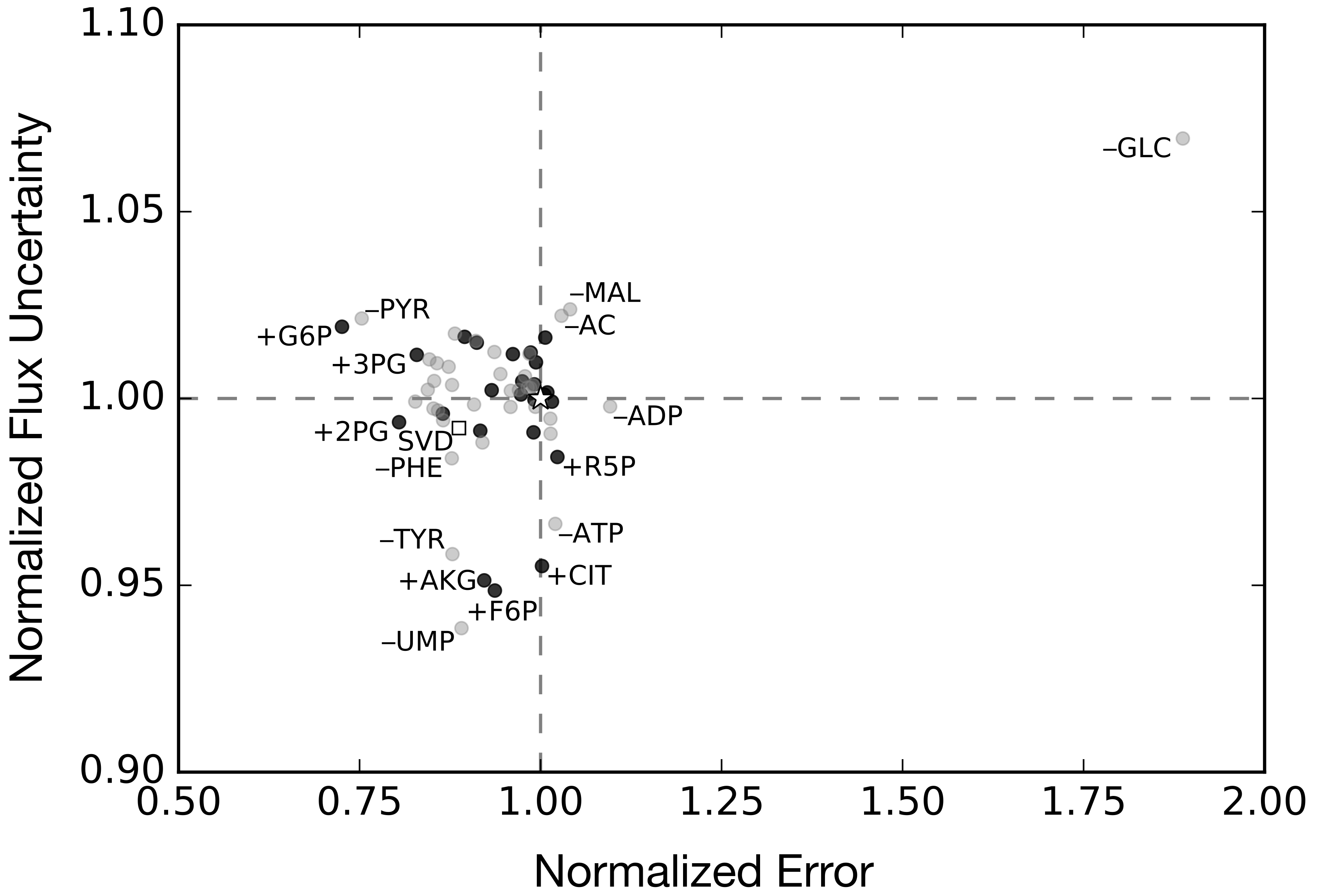
The base synthetic data set, consisting of 36 metabolite time series and the protein product CAT, was the measurement set used to train the kinetic model of Horvath et al. [32]. Thus, the confidence intervals on the synthetic data used in this study as constraints on the flux estimation problem were informed by experimental measurements of glucose, organic and amino acids, energy species and the protein product CAT. However, we have no a priori reason to suppose that this experimental design was optimal. Toward this question, we performed simulations and flux variability analysis (FVA) for alternative synthetic data sets to understand the importance of measurement selection when characterizing CFPS (Figure 5 and Figure 6). In all cases, we assumed the same sampling frequency as the base synthetic dataset, but we varied which species were measured. First, we removed each of the 37 metabolites from the base set, one at a time, to create 37 measurement exclusion sets, consisting of 36 metabolites each (Figure 5, light gray dots). For each set, the state the dynamic model was used to calculate a value of error against the synthetic data, and FVA was used to calculate a value of flux uncertainty. Most of the exclusion sets clustered around the base case, with error values between 75% and 110%, and flux uncertainties between 93% and 103%, of the base case. The exception to this was the glucose exclusion set, which showed 89% higher error and 7% greater flux uncertainty. Within the primary cluster, a slight pattern emerged: the sets in which an organic acid were removed tended to result in increased error, while the removal of an amino acid tended to reduce error; however, this was not true across all metabolites. We also performed the analysis on several inclusion sets to determine which additional metabolites could improve predictive power (Figure 5, black dots). In particular, we added unmeasured central carbon metabolites to the base case, which resulted in 23 inclusion sets, consisting of 38 metabolites each. As with the exclusion sets, most of the inclusion sets clustered around the base case, with error values between 72% and 103%, and flux uncertainties between 94% and 102%, of the base case. Considering all exclusion and inclusion sets, there was generally no correlation between the metabolite prediction error and flux uncertainty. Taken together, these suggested central carbon metabolites, especially glucose, were important to characterize the network, but performing single additional measurements was not enough to significantly increase predictive power. Next, we explored whether measurement selection could be based upon the structural features of a metabolic network. Toward this question, we used singular value decomposition (SVD) of the stoichiometric matrix to suggest which metabolites should be measured.

Singular value decomposition (SVD) measurement selection outperformed the base case, with a prediction error improvement of 11% and similar flux variability (Figure 5, open square). SVD was used to decompose the stoichiometric matrix into 105 modes. The top 36 metabolites that had the greatest weighted sum across the modes that accounted for 95% of the network were estimated. Since our exclusion analysis identified glucose as the single most important metabolite, we added it to the top metabolites as determined by SVD to obtain a 37-metabolite constraint set, consisting of: GTP, GDP, GMP, ATP, ADP, AMP, UTP, UMP, CTP, CMP, GLN, GLU, ASP, LYS, LEU, HIS, THR, PHE, ALA, VAL, TYR, GLY, SER, H, ASN, ILE, MET, AKG, PYR, ARG, CYS, NH3, FUM, SUCC, TRP, ACCOA, and glucose. The SVD measurement set suggested that energy, and amino acid species carried the most information compared to central carbon species, which made up a relatively smaller fraction of the list. Surprisingly, the measurement set selected by SVD was approximately 80% similar to the original synthetic data generated by hand. However, the 20% difference was enough to improve the prediction error by approximately 11%. Taken together, measurements selected by SVD decomposition of the stoichiometric matrix improved the prediction of metabolite abundance, but SVD-based measurement selection did not improve flux variability.

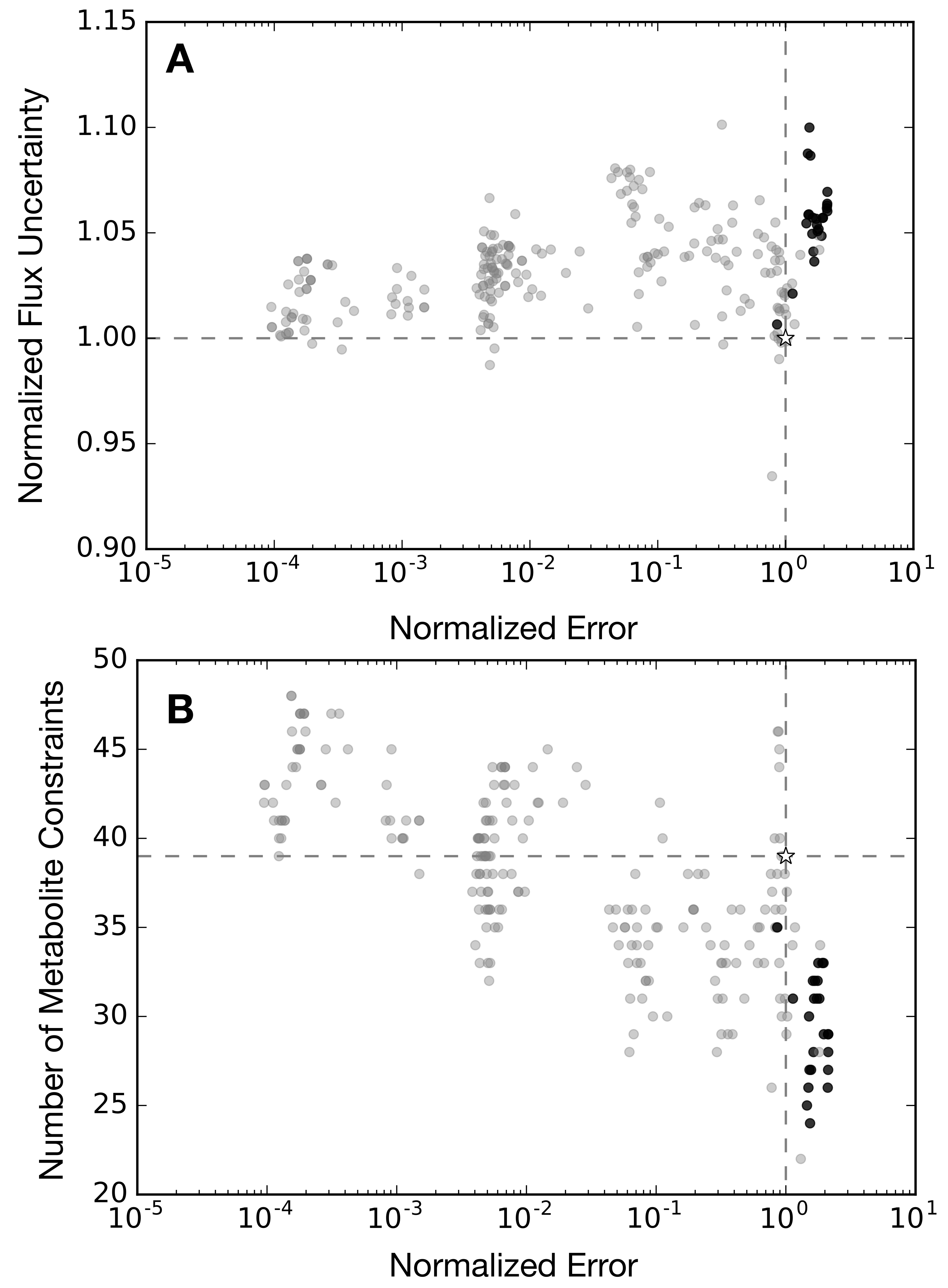
Next, we used heuristic optimization to systematically investigate the effect of changing the dimension and identify the measurement constraints (Figure 6). In particular, we minimized the error and flux variability of model predictions by varying the metabolites that appeared in the synthetic constraint set. We used a binary simulated annealing algorithm to switch metabolite membership in the constraint set on or off, and thus generated an ensemble of >200 measurement constraint sets (Figure 6A). While there was no strict error threshold, the simulated annealing algorithm was less likely to accept high-error sets into the ensemble; thus, the error of most sets in the ensemble was less than that of the base case. Specifically, the error varied from just over double to less than one ten-thousandth of the base case. Flux uncertainty was also a component of the objective function, but was only improved by 7%, suggesting this performance metric was tightly constrained; network flux values were not well characterized, even with comprehensive training datasets. As expected, there was an inverse relationship between the number of metabolite constraints and the prediction error (Figure 6B). However, the slope of that trend was striking; error was improved by three to four orders of magnitude, simply by increasing the number of constraints by 11 or fewer. Furthermore, the base synthetic measurement set was outperformed by the majority of the ensemble; often, the simulated annealing approach achieved the same error with fewer constraints, or much lower error with the same, or even fewer, constraints. This suggests that, while comprehensive, the original synthetic dataset was not optimal in terms of predictive power per measurement. However, the base case was one of the best in terms of reducing flux uncertainty.

Lastly, we investigated which metabolites were most effective at improving predictive power by considering how often it appeared in the ensemble (

Table 4. Metabolites by frequency of appearance in the simulated annealing constraint sets.

Metabolite	Symbol	Frequency
alpha-D-Glucose	GLC	89.9%
Glucose 6-phosphate	G6P	89.9%
Citrate	CIT	85.7%
Isocitrate	ICIT	84.9%
Fumarate	FUM	84.5%
Fructose 6-phosphate	F6P	83.6%
6-Phospho-D-glucono-1,5-lactone	6PGL	81.5%
sedo-Heptulose 7-phosphate	S7P	79.4%
Alanine	ALA	77.7%
Guanosine triphosphate	GTP	77.3%
Malate	MAL	75.6%
D-Ribulose 5-phosphate	RU5P	74.8%
Erythrose 4-phosphate	E4P	73.1%
Adenosine diphosphate	ADP	72.3%
alpha-Ketoglutarate	AKG	71.8%
Uridine diphosphate	UDP	70.2%
Succinate	SUCC	69.7%
Cytidine monophosphate	CMP	69.3%
Guanosine diphosphate	GDP	67.2%
6-Phospho-D-gluconate	6PGC	67.2%
Arginine	ARG	66.8%
Ribose 5-phosphate	R5P	66.4%
Methionine	MET	65.5%
Glyoxylate	GLX	65.5%
Glutamine	GLN	63.9%
Phenylalanine	PHE	63.4%
Valine	VAL	62.6%
Glyceraldehyde 3-phosphate	G3P	62.2%
Adenosine monophosphate	AMP	62.2%
Proline	PRO	60.1%
Fructose 1,6-diphosphate	FDP	60.1%
Dihydroxyacetone phosphate	DHAP	60.1%
Histidine	HIS	59.7%
Glycine	GLY	59.7%
Oxaloacetate	OAA	58.4%
2-Dehydro-3-deoxy-D-gluconate 6-phosphate	2DDG6P	58.4%
Chloramphenicol acetyltransferase	CAT	56.3%
Cysteine	CYS	55.5%
Acetate	AC	54.2%
Succinyl coenzyme A	SUCCOA	53.8%
Uridine monophosphate	UMP	52.9%
Tryptophan	TRP	52.5%
Lactate	LAC	52.5%
Uridine triphosphate	UTP	52.1%
Aspartate	ASP	51.7%
Guanosine monophosphate	GMP	50.8%
Asparagine	ASN	50.4%
Cytidine diphosphate	CDP	50.0%
Phosphoenolpyruvate	PEP	48.3%
3-Phosphoglycerate	3PG	47.9%
2-Phosphoglycerate	2PG	47.1%
Lysine	LYS	43.3%
Threonine	THR	42.0%
Glutamate	GLU	38.7%
Tyrosine	TYR	37.0%
Adenosine triphosphate	ATP	37.0%
D-Xylulose 5-phosphate	XU5P	35.7%
Acetyl coenzyme A	ACCOA	34.9%
Cytidine triphosphate	CTP	33.2%
Serine	SER	31.9%
Isoleucine	ILE	29.8%
Leucine	LEU	26.5%
Pyruvate	PYR	21.8%

). Glucose unsurprisingly appeared most often (tied with G6P), but interestingly was not in every constraint set. Those that did not contain glucose had some of the highest errors, but also some of the smallest constraint set sizes (Figure 6B, black dots). The most frequent metabolites from the heuristic method were largely from glycolysis, pentose phosphate, and the TCA cycle (compared to the SVD analysis which gave greater consideration to energetic and amino acid species). To further understand the species selection, we calculated the frequency of appearance in the 57 best sets, those with error of least three orders of magnitude lower than the base case (

Table 5. Metabolites by frequency of appearance in the 57 best simulated annealing constraint sets, those with error at least three orders of magnitude lower than the base synthetic dataset.

Metabolite	Symbol	Frequency
D-Xylulose 5-phosphate	XU5P	100%
sedo-Heptulose 7-phosphate	S7P	100%
D-Ribulose 5-phosphate	RU5P	100%
Ribose 5-phosphate	R5P	100%
Oxaloacetate	OAA	100%
Isocitrate	ICIT	100%
alpha-D-Glucose	GLC	100%
Glucose 6-phosphate	G6P	100%
Glyceraldehyde 3-phosphate	G3P	100%
Fumarate	FUM	100%
Fructose 1,6-diphosphate	FDP	100%
Fructose 6-phosphate	F6P	100%
Erythrose 4-phosphate	E4P	100%
Dihydroxyacetone phosphate	DHAP	100%
Citrate	CIT	100%
Alanine	ALA	100%
6-Phospho-D-glucono-1,5-lactone	6PGL	100%
6-Phospho-D-gluconate	6PGC	100%
2-Dehydro-3-deoxy-D-gluconate 6-phosphate	2DDG6P	100%
Uridine triphosphate	UTP	98.2%
alpha-Ketoglutarate	AKG	98.2%
Succinate	SUCC	94.7%
Arginine	ARG	94.7%
3-Phosphoglycerate	3PG	94.7%
Guanosine triphosphate	GTP	91.2%
Uridine monophosphate	UMP	89.5%
Glutamine	GLN	87.7%
Cytidine monophosphate	CMP	87.7%
Tyrosine	TYR	82.5%
Threonine	THR	82.5%
Aspartate	ASP	80.7%
Cytidine diphosphate	CDP	75.4%
Uridine diphosphate	UDP	71.9%
Valine	VAL	70.2%
Methionine	MET	68.4%
Guanosine monophosphate	GMP	68.4%
Glycine	GLY	68.4%
Adenosine diphosphate	ADP	68.4%
Tryptophan	TRP	61.4%
Phenylalanine	PHE	59.6%
Acetate	AC	57.9%
Malate	MAL	52.6%
Phosphoenolpyruvate	PEP	50.9%
Leucine	LEU	49.1%
Proline	PRO	47.4%
Isoleucine	ILE	47.4%
Histidine	HIS	47.4%
Adenosine monophosphate	AMP	45.6%
Glyoxylate	GLX	43.9%
Lactate	LAC	40.4%
Chloramphenicol acetyltransferase	CAT	38.6%
Cysteine	CYS	36.8%
Asparagine	ASN	35.1%
Pyruvate	PYR	33.3%
Glutamate	GLU	31.6%
Succinyl coenzyme A	SUCCOA	22.8%
Guanosine diphosphate	GDP	22.8%
2-Phosphoglycerate	2PG	22.8%
Cytidine triphosphate	CTP	14%
Acetyl coenzyme A	ACCOA	14%
Lysine	LYS	7%
Adenosine triphosphate	ATP	5.3%
Serine	SER	0%

). Nineteen metabolites appeared in all of these sets, and all but Alanine were central carbon metabolites (defined here as glycolysis, pentose phosphate, TCA). Taken together, measurement selection made a significant difference in capturing dynamic metabolite abundance in cell-free protein synthesis. Although the error decreased with increasing measurement number overall, the specific combination of metabolites was arguably even more important. Metabolic fluxes, however, remained unknown despite the large number of measurements taken.

3. Discussion

In this study, we presented a dynamic constraint-based model of cell-free protein expression. This approach avoids the pseudo-steady-state assumption found in traditional constraint-based approaches, which allowed for the direct integration of metabolite measurements into the flux estimation problem, and the the accumulation or depletion of network metabolites. The approach used the E. coli cell-free protein synthesis metabolic network from Vilkhovoy and coworkers [31], and the simulated metabolite trajectories from the kinetic model of Horvath et al. [32] as constraints on the CFPS flux calculation. The dynamic constraint-based model satisfied time-dependent metabolite measurement constraints, predicted unconstrained metabolite concentrations as well as the concentration of a model protein, chloramphenicol acetyltransferase (CAT). Model interrogation suggested the most important metabolite measurement within the dataset to be glucose, as excluding the glucose yielded the greatest metabolite prediction error, and the greatest uncertainty in the estimated metabolic flux. Furthermore, we evaluated metabolite constraint sets with one more and one fewer metabolites than the base case (37 metabolites) to explore the impact of measurement selection on model performance. The single addition of metabolites yielded no significant improvement in the predictive power, while the single exclusion suggested glucose to be the most important measured metabolite in the base case. Next, we selected measurement species based on the results of singular value decomposition on the stoichiometric matrix. The top 36 species from the SVD analysis with the addition of glucose improved the predictive power and reduced flux uncertainty compared with the base case. Finally, we described a heuristic optimization approach to estimate the optimal list of metabolite measurements. Measurement sets determined by heuristic optimization vastly outperformed the accuracy of the base synthetic dataset; model precision, meanwhile, was virtually unchanged despite comprehensive measurement sets. Taken together, model interrogation showed that, even with a comprehensive dataset, there still exists a great amount of uncertainty associated with metabolic fluxes. This highlights the need for fluxomic data to fully understand biological networks.

Despite synthetic datasets consisting of greater than 30 metabolite time series, estimates of metabolic flux were largely uncertain. Flux variability analysis suggested that the metabolite constraints could be met with a wide range of different flux distributions. For instance, an open question in cell-free systems is the balance between glycolytic versus pentose phosphate pathway flux. In previous studies of E. coli cell-free protein synthesis, the kinetic model of Horvath and coworkers suggested that glucose was consumed primarily by glycolytic reactions, with minimal flux into the pentose phosphate pathway. However, Vilkhovoy et al. estimated, using sequence specific flux balance analysis with the same experimental dataset, that the CAT production was unaffected by the choice of pentose phosphate pathway versus glycolysis; deletion of either pathway did not change protein productivity. To answer this discrepancy, model analysis showed, during the first phase when glucose was being consumed, glycolytic and pentose phosphate fluxes (pgi and zwf, respectively) exhibited large uncertainty, as either could be utilized to satisfy CAT production. The measurement selection analysis was conducted by excluding or including a metabolite from the constraint set. The exclusion sets were dominated by the removal of glucose, and to a lesser extent the organic acids, suggesting that measurements of central carbon metabolism intermediates were more important than energetic and amino acid measurements. However, the inclusion sets showed no significant effect on error and flux uncertainty. There was generally no correlation between the error and flux uncertainty of a model constrained to a particular metabolite set, except with respect to the outlier glucose. Model calculations showed that, even with a comprehensive data set of 37 metabolite measurements, there was significant flux uncertainty. This suggested that there were many flux combinations that could give rise to the same set of time course measurements. This phenomenon was further supported by analyzing the ensemble of constraint sets determined by heuristic optimization. Although the optimization algorithm reduced the objective function by four degrees of magnitude, the flux variability remained stagnant in comparison. An ensemble of measurement sets ranging from 22 to 48 metabolite constraints was only able to reduce flux uncertainty by 7% from the base synthetic data set. The dynamic constraint-based model showed high flux variability in important branch points, including the glucose-6-phosphate split between glycolysis and pentose phosphate, the 6PGC split into pentose phosphate and Entner–Doudoroff, and the pyruvate split into TCA cycle versus lactate production. This may be why the high overall flux variability was robust to the varying of metabolite constraints. Using three different sampling approaches (single additions/exclusions, singular value decomposition, simulated annealing) coupled with the dynamic constraint-based model, we estimated key metabolites that could be prioritized in measurement selection, such as glucose. Although measuring central carbon metabolites and amino acids is the intuition of most researchers, model interrogation was able to provide the importance of certain species over others; for instance, measuring G6P, G3P, and F6P would be more fruitful than measuring PEP. Interestingly, many of the most valuable measurements were involved in upper glycolysis and pentose phosphate, such as glucose, G6P, and 6PGL. This may be because upstream metabolites have an effect on more of the network; any error or uncertainty in these metabolites will cascade down the rest of the network and magnify throughout. Taken together, the dynamic constraint-based model quantitatively affirmed the robustness of metabolism, and illustrated the complexity of inferring flux information from metabolite concentrations. Ultimately, to determine the metabolic flux distribution occurring in a cell-free system, we need to add additional constraints to the flux estimation calculation. This study suggested that metabolite measurements alone were not sufficient. However, these are not the only experimentally realizable types of constraints. For example, thermodynamic feasibility constraints may result in a better depiction of the flux distribution [37,38], and ${}^{13}$C labeling constraints in cell-free systems could provide significant insight. However, while ${}^{13}$C labeling techniques are well established for in vivo processes [39], application of these techniques to cell-free systems remains an active area of research.

The use of cell-free systems as a personalized point of care biomanufacturing tools, as platforms for vaccine development, or as the basis for portable pathogen detection are promising research directions [1,40,41,42,43]. cell-free systems have significant advantages in these application areas compared to in vivo systems. For example, as there is no longer a cell wall, we can experimentally observe the system and intervene if need be. Moreover, cell-free synthetic circuitry is highly portable. For example, it can be dried onto paper, easily transported, and potentially stored indefinitely [44]. Thus, after development and testing of the circuitry, and manufacturing of the devices, there is no need for large, bulky and expensive equipment usually associated with in vivo bioprocesses. However, to move beyond proof of concept and into industrial or medical practice will require extensive optimization. Mathematical modeling is an important tool in this regard. In this study, we explored the relationship between measurement selection and the ability to estimate metabolic flux in a cell-free system. One of the central advantages of cell-free systems is the ability to measure the concentration of metabolic intermediates. However, ultimately, we need to transform these measurements into testable hypothesis about the performance of a cell-free system. The connection between flux estimation and optimal measurement selection has been well studied for in vivo systems; for example, see the classic work of Savinell and Palsson [45,46]. Moreover, the robust quantification of metabolic flux in in vivo systems is also well developed, with both mature experimental and computational tools available (see [39,47,48]). However, quantification of metabolic flux in cell-free systems from metabolite measurements remains an open area of research. Certainly, techniques developed for the identification and quantification of in vivo systems could be applied to cell-free. For example, Lucks and coworkers used the D-optimal experimental design approach of Doyle and coworkers [49] to parameterize a kinetic model of RNA-based cell-free circuits [33]. However, Lucks and coworkers did not consider the resources required for the RNA circuits to function. Quantification of metabolic flux, and the associated resource production and consumption in cell-free applications, is not common. Instead, the synthetic biology community has focused on designing circuits and circuit components with specific behaviors e.g., [50,51,52], assuming the resources required to express these components will be available. At proof of concept scales, this is a reasonable assumption. However, as we move toward industrial practice, careful attention must be paid to resource generation and consumption—for example, optimizing the expressed proteome for cell-free extract production, or balancing cofactor utilization during the cell-free reaction [53,54]. Resource management has a direct impact on the performance and industrial viability of cell-free applications—for example, potentially limiting the rate of production and yield of circuit components, the size and complexity of possible synthetic circuits, the operational lifetime of synthetic devices, or the titer and rate of production of protein and small molecule products. Thus, as we move beyond technology development to realistic industrial or medical applications, the performance of synthetic devices will become increasingly important. Toward this need, we expect mathematical modeling will play an important role.

4. Materials and Methods

4.1. Formulation and Solution of the Model Equations

We modeled the time evolution of the ith metabolite concentration ($x_i$), the scaled activity of network enzymes (${ϵ}_i$), transcription processes generating the mRNA m and translation processes generating the protein $\mathcal{P}$ in an E. coli cell-free metabolic network as a system of ordinary differential equations:

$$\begin{array}{ccc}\hfill {\dot{x}}_i& =& \sum _{j=1}^{\mathcal{R}}{\sigma }_{ij}{r}_j\left(\mathbf{x},ϵ,\mathbf{k}\right)i=1,2,\cdots ,\mathcal{M},\hfill \end{array}$$

(1)

$$\begin{array}{ccc}\hfill {\dot{ϵ}}_i& =& -{\lambda }_i{ϵ}_{i}i=1,2,\cdots ,\mathcal{N},\hfill \end{array}$$

(2)

$$\begin{array}{ccc}\hfill \dot{m}& =& r_T-\lambda m,\hfill \end{array}$$

(3)

$$\begin{array}{ccc}\hfill \dot{\mathcal{P}}& =& r_X.\hfill \end{array}$$

(4)

The quantity $\mathcal{R}$ denotes the number of metabolic reactions, $\mathcal{M}$ denotes the number of metabolites and $\mathcal{N}$ denotes the number of metabolic enzymes in the model. The quantity $r_j\left(\mathbf{x},ϵ,\mathbf{k}\right)$ denotes the rate of reaction j. Typically, reaction j is a nonlinear function of metabolite and enzyme abundance, as well as unknown kinetic parameters $\mathbf{k}$ ($\mathcal{K}\times 1$). The quantity ${\sigma }_{ij}$ denotes the stoichiometric coefficient for species i in reaction j. If ${\sigma }_{ij}>0$, metabolite i is produced by reaction j. Conversely, if ${\sigma }_{ij}<0$, metabolite i is consumed by reaction j, while ${\sigma }_{ij}=0$ indicates metabolite i is not connected with reaction j. Lastly, ${\lambda }_i$ denotes the scaled enzyme activity decay constant. The system material balances were subject to the initial conditions $\mathbf{x}\left(t_o\right)={\mathbf{x}}_o$ and $ϵ\left(t_o\right)=\mathbf{1}$ (initially, we have 100% cell-free enzyme activity).

The cell-free model equations were solved using a dynamic constraint-based approach in which the rates of the metabolic fluxes, transcription and translation processes were estimated by solving an optimization subproblem from t to $t+\Delta t$. In particular, the biochemical fluxes $r_1,r_2,\cdots ,r_{\mathcal{R}}$ which appear in the balance equations were calculated from t to $t+\Delta t$ by solving a constrained optimization subproblem with (potentially nonlinear) objective $\mathcal{O}\left(x_1,x_2,\cdots ,x_{\mathcal{M}}\right)$:

$$\underset{r_1,r_2,\cdots ,r_{\mathcal{R}}}{max}\mathcal{O}\left(x_1,x_2,\cdots ,x_{\mathcal{M}}\right)$$

(5)

subject to species constraints and flux bounds:

$$\begin{array}{ccc}\hfill \left(\sum _{j=1}^{\mathcal{R}}{\sigma }_{ij}{r}_j-{\dot{x}}_i\right)& \ge & 0i=1,2,\cdots ,\mathcal{M},\hfill \end{array}$$

(6)

$$\begin{array}{ccc}\hfill 0\le r_j& \le & {\mathcal{U}}_j\left(x_1,x_2,\cdots ,x_{\mathcal{M}},\kappa \right)j=1,2,\cdots ,\mathcal{R}.\hfill \end{array}$$

(7)

In this study, we maximized the rate of translation $r_X$ unless otherwise specified. We discretized the derivative term for each species using a constant width h forward different approximation (however, this was done for convenience and more sophisticated techniques could have been used). The reaction bounds ${\mathcal{U}}_j\left(x_1,x_2,\cdots ,x_{\mathcal{M}},\kappa \right)$ are potentially non-linear functions of the system state, and can be updated during each time step. Here, we modeled the upper bound for flux j as ${\widehat{V}}_{max}{ϵ}_j\left(k\right)$, where ${\widehat{V}}_{max}$ denotes a characteristic maximum reaction velocity, and ${ϵ}_j\left(k\right)$ denotes the scaled enzyme activity catalyzing reaction j at time step k. The characteristic maximum reaction velocity was set to 600 mM/h (which corresponds to an average $k_{cat}\simeq$ 1000 s${}^{-1}$ and and enzyme concentration of approximately 0.2 $\mathsf{\mu }$M) unless otherwise specified. Additional species constraints can be added to directly incorporate metabolomic, proteomic or transcriptomic measurements into the flux calculation. In this study, we incorporated metabolite measurement constraints of the form:

$${\chi }_{m,k+1}^L\le x_{m,k+1}\le {\chi }_{m,k+1}^{U}m=1,2,\cdots ,\Xi ,$$

(8)

where ${\chi }_{m,k+1}^L$ and ${\chi }_{m,k+1}^U$ denote the lower and upper measurement bound for metabolite m at time step $k+1$, where $\Xi$ metabolites were measured over the time course of the cell-free reaction. Lastly, we imposed a user-configurable bound ${\mathcal{B}}_i$ on the maximum rate of change for metabolite i:

$$\left|{\dot{x}}_i\right|\le {\mathcal{B}}_{i}i=1,2,\cdots ,\mathcal{M}$$

(9)

and non-negativity constraints $x_i\ge 0$ for all metabolites and all time steps.

The bounds on the transcription rate (${\mathcal{L}}_T=r_T={\mathcal{U}}_T$) were modeled as:

$$r_T=V_T^{max}\left(\frac{G_{\mathcal{P}}}{K_T+G_{\mathcal{P}}}\right),$$

(10)

where $G_{\mathcal{P}}$ denotes the concentration of the gene encoding the protein of interest, and $K_T$ denotes a transcription saturation coefficient. The maximum transcription rate $V_T^{max}$ was formulated as:

$$V_T^{max}\equiv \left[R_T\left(\frac{{\dot{v}}_T}{l_G}\right)u\left(\kappa \right)\right],$$

(11)

where $R_T$ denotes the RNA polymerase concentration (nM), ${\dot{v}}_T$ denotes the RNA polymerase elongation rate (nt/h), $l_G$ denotes the gene length (nt). The term $u\left(\kappa \right)$ (dimensionless, $0\le u\left(\kappa \right)\le 1$) is an effective model of promoter activity, where $\kappa$ denotes promoter specific parameters. The general form for the promoter models was taken from Moon et al. [55], which was based on earlier studies from Bintu and coworkers [56], and similar to the genetically structured modeling approach of Lee and Bailey [57]. In this study, we considered only the T7 promoter model:

$$u_{T7}=\frac{K_{T7}}{1+K_{T7}},$$

(12)

where $K_{T7}$ denotes a T7 RNA polymerase binding constant. The values for all promoter parameters are given in Table 1.

The translation rate ($r_X$) was bounded by:

$$0\le r_X\le V_X^{max}\left(\frac{m}{K_X+m}\right),$$

(13)

where $\mathrm{m}$ denotes the mRNA abundance and $K_X$ denotes a translation saturation constant.

The maximum translation rate $V_X^{max}$ was formulated as:

$$V_X^{max}\equiv \left[K_P{R}_X\left(\frac{{\dot{v}}_X}{l_P}\right)\right].$$

(14)

The term $K_P$ denotes the polysome amplification constant, ${\dot{v}}_X$ denotes the ribosome elongation rate (amino acids per hour), and $l_P$ denotes the number of amino acids in the protein of interest. The mRNA abundance $\mathrm{m}$ was estimated as:

$$m_{k+1}=m_k+(r_T-m_k\lambda )h,$$

(15)

where $\lambda$ denotes the mRNA degradation rate constant (h${}^{-1}$). All translation parameters are given in Table 1.

Metabolic fluxes were estimated at each time step using the GNU Linear Programming Kit (GLPK) v4.55 [58]. The objective of the optimization subproblem was to maximize the translation rate, subject to the stoichiometric and metabolite constraints. The model code, parameters and initial conditions used in this study are available under an MIT software license at the Varnerlab website [35]. The model code is written in the Julia programming language [59]. Default transcription and translation parameters are stored in TXTLDictionary.jl, while specific simulations are described in the Solve_*.jl files. Lastly, the figures for this study were produced using the Plot_*.jl scripts.

4.2. Sampling of Transcription and Translation Parameters

The influence of the uncertainty in the transcription (TX) and translation (TL) parameters was estimated by sampling the expected physiological ranges for these parameters as determined from literature. We generated uniform random samples between an upper (u) and lower (l) parameter bound of the form:

$$p^{*}=l+(u-l)\times \mathcal{U}\left(0,1\right),$$

(16)

where $\mathcal{U}\left(0,1\right)$ denotes a uniform random number between 0 and 1. The T7 RNA polymerase concentration was sampled between 800 and 1200 nM, ribosome levels between 1.5 and 3.0 $\mathsf{\mu }$M, polysome amplification between 5 and 15, the RNA polymerase elongation rate between 20 and 30 nt/s, and the ribosome elongation rate between 1.0 and 3.0 aa/s [10,60]; see TXTL_ensemble.jl for a complete list of parameter ranges.

4.3. Generation and Evaluation of Alternative Measurement Sets

The measurement sets consisted of the base (one set of 37 metabolites), inclusion sets (23 sets of 38 metabolites each), exclusion sets (37 sets of 36 metabolites each), SVD-guided (one set of 37 metabolites), and simulated annealing samples (238 sets of varying length). In all cases, we assumed the same sampling frequency as the base synthetic dataset, but we varied which species were measured. The exclusion or inclusion measurement sets were constructed by removing or adding a metabolite to the base set, while the SVD-guided measurement set was constructed from high importance metabolites; the top 36 metabolites (plus glucose) that had the greatest singular value weighted sum across the SVD-modes, accounting for 95% of the network structure, were designated the SVD measurement set. Lastly, we used simulated annealing to generate potentially optimal measurements sets, where the objective was to minimize the product of the prediction error, and flux uncertainty. The prediction error, $\mathcal{E}$, was computed by comparing the simulated versus the measured value of a metabolite, for a ${\mathcal{M}}_{\mathrm{core}}$ set of metabolites. On the other hand, the flux variability was computed using flux variability analysis (FVA) [61], subject to constraints on the CAT production rate, and the selected metabolite trajectories. In particular, the metabolite prediction error was calculated from the time-dependent state array:

$$\mathcal{E}=\sum _{i=1}^{{\mathcal{M}}_{\mathrm{core}}}\sum _{t=t_i}^{\mathcal{T}}\left(max\left(x_i\left(t\right)-y_i^U\left(t\right),0\right)+max\left(y_i^L\left(t\right)-x_i\left(t\right),0\right)\right),$$

where $x_i\left(t\right)$ denotes the simulated value of metabolite i at time t, $y_i^U\left(t\right)$ denotes the upper bound of the 95% confidence interval on the synthetic data for metabolite i at time t, $y_i^L\left(t\right)$ denotes the lower bound of the 95% confidence interval on the synthetic data for metabolite i at time t, and ${\mathcal{M}}_{\mathrm{core}}$ denotes the subset of metabolites in the core metabolism. For this calculation, the entire time course was considered ($t_i$ = 0 h, $\mathcal{T}$ = 3 h). The flux uncertainty was calculated from the maximal and minimal flux arrays:

$$\begin{array}{ccc}\hfill {\sigma }_{\mathrm{overall}}& =& \sum _{r_j\in {\mathcal{R}}_{\mathrm{core}}}\sum _{t=t_i}^{\mathcal{T}}{\left(r_j^{\max }\left(t\right)-r_j^{\min }\left(t\right)\right)}^2,\hfill \end{array}$$

where $r_j^{\max }\left(t\right)$ denotes the maximum value of flux j, while $r_j^{\min }\left(t\right)$ denotes the value of flux j at time t, calculated using flux variability analysis. The quantity ${\mathcal{R}}_{\mathrm{core}}$ denotes the subset of reactions that constitute the core metabolism. For the flux uncertainty calculations, either the entire reaction time course was considered ($t_i$ = 0 h, $\mathcal{T}$ = 3 h), or the uncertainty was calculated separately for each phase (phase 1: $t_i$ = 0 h, $\mathcal{T}$ = 1 h; phase 2: $t_i$ = 1 h, $\mathcal{T}$ = 3 h).

The simulated annealing algorithm began by evaluating the error and flux uncertainty of the base case and multiplying these to obtain a cost function:

$$\mathtt{cost}=\mathcal{E}·{\sigma }_{\mathrm{overall}}.$$

(17)

Then, each metabolite that was considered measurable was added to or removed from the constraint set with a certain probability $p_{switch}$:

$${\theta }_i^{\mathrm{new}}=\left\{\begin{array}{cc}1-{\theta }_i,\hfill & \mathcal{U}\left(0,1\right)<p_{switch},\hfill \\ {\theta }_i,\hfill & \mathcal{U}\left(0,1\right)>p_{switch},\hfill \end{array}\right.i=1,2,\cdots ,{\mathcal{M}}_{\mathrm{measurable}},$$

(18)

where ${\theta }_i\in \{0,1\}$ denotes a binary parameter encoding whether or not metabolite i is in the constraint set, $\mathcal{U}\left(0,1\right)$ denotes a uniform random number taken from a distribution between 0 and 1, and ${\mathcal{M}}_{\mathrm{measurable}}$ denotes the set of metabolites deemed to be measurable. For each newly generated constraint set, we re-solved the dFBA and FVA problems, and re-calculated the cost function. All sets with a lower cost were accepted into the ensemble. Sets with a higher cost were also accepted into the ensemble, if they satisfied the acceptance constraint:

$${\mathcal{R}}_{0,1}^{\mathrm{uniform}}<exp\left(-\alpha ·\frac{{\mathtt{cost}}_{\mathtt{new}}-\mathtt{cost}}{\mathtt{cost}}\right),$$

(19)

where ${\mathcal{R}}_{0,1}^{\mathrm{uniform}}$ denotes a random number taken from a uniform distribution between 0 and 1, $\mathtt{cost}$ denotes the cost of the current parameter set, $\mathtt{cost}$new denotes the cost of the new parameter set, and $\alpha$ denotes an adjustable parameter to control the tolerance to high-error sets. A total of 238 samples were accepted into the ensemble, of which there were 219 unique sets. Both ${\mathcal{M}}_{\mathrm{core}}$ and ${\mathcal{R}}_{\mathrm{core}}$ and user-configurable are defined in the model code repository available from the Varnerlab website [35].

5. Conclusions

In summary, we used a dynamic constraint-based modeling approach to simulate cell-free metabolism, and to study how measurement selection impacts model performance. We extended sequence specific flux balance analysis, by removing the pseudo steady state assumption, and adding synthetic metabolite measurement constraints to the flux calculation. Using this method, we simulated the cell-free synthesis of a model protein, chloramphenicol acetyltransferase, we identified the most important measured species in the cell-free system, and additional species that yielded the lowest metabolite prediction error and flux uncertainty. Only synthetic metabolite measurements were used in this study; however, this work built a foundation to rationally design experimental measurement protocols that could be implemented with a variety of analytical techniques. Taken together, these findings represent a novel tool for dynamic cell-free simulations, measurement selection and pathway analysis, not only for E. coli, but potentially for align variety of metabolic networks, whether in vivo or cell-free. However, while this first study was promising, there were several issues to consider in future work. First, while we described transcription and translation at a sequence specific level, we have not considered the complexities of protein folding, or post-translational modifications such as protein glycosylation. A more detailed description of transcription and translation reactions, including the role of chaperones in protein folding, has been used in in-vivo genome scale ME models; e.g., see O’Brien et al. [20]. These template reactions could easily be adapted to a cell-free system, thereby providing a potentially higher fidelity description protein synthesis and folding. Next, the inclusion of post-translational modifications such as protein glycosylation in the next generation of models will be important to describe the cell-free synthesis of therapeutic proteins. DeLisa and coworkers recently showed that glycoproteins can be synthesized in a cell-free system, using extract generated from modified E. coli cells capable of asparagine-linked protein glycosylation [62]. Simulation of the generation and attachment of glycans to protein targets could be an important step to optimizing cell-free glycoprotein production. Lastly, while we modeled the cell-free production of a only single protein in this study, sequence specific dynamic constraint models could be developed for multi-protein synthetic circuits, RNA circuits or even small molecule production. Thus, this approach offers a unique tool to model and potentially optimize a wide variety of application areas in synthetic biology.

References

- Pardee, K.; Slomovic, S.; Nguyen, P.Q.; Lee, J.W.; Donghia, N.; Burrill, D.; Ferrante, T.; McSorley, F.R.; Furuta, Y.; Vernet, A.; et al. Portable, On-Demand Biomolecular Manufacturing. Cell 2016, 167, 248–259. [Google Scholar] [CrossRef] [PubMed]
- Jewett, M.C.; Calhoun, K.A.; Voloshin, A.; Wuu, J.J.; Swartz, J.R. An integrated cell-free metabolic platform for protein production and synthetic biology. Mol. Syst. Biol. 2008, 4, 220. [Google Scholar] [CrossRef] [PubMed]
- Matthaei, J.H.; Nirenberg, M.W. Characteristics and stabilization of DNAase-sensitive protein synthesis in E. coli extracts. Proc. Natl. Acad. Sci. USA 1961, 47, 1580–1588. [Google Scholar] [CrossRef] [PubMed]
- Nirenberg, M.W.; Matthaei, J.H. The dependence of cell-free protein synthesis in E. coli upon naturally occurring or synthetic polyribonucleotides. Proc. Natl. Acad. Sci. USA 1961, 47, 1588–1602. [Google Scholar] [CrossRef] [PubMed]
- Spirin, A.; Baranov, V.; Ryabova, L.; Ovodov, S.; Alakhov, Y. A continuous cell-free translation system capable of producing polypeptides in high yield. Science 1988, 242, 1162–1164. [Google Scholar] [CrossRef] [PubMed]
- Kim, D.M.; Swartz, J.R. Regeneration of adenosine triphosphate from glycolytic intermediates for cell-free protein synthesis. Biotechnol. Bioeng. 2001, 74, 309–316. [Google Scholar] [CrossRef] [PubMed]
- Lu, Y.; Welsh, J.P.; Swartz, J.R. Production and stabilization of the trimeric influenza hemagglutinin stem domain for potentially broadly protective influenza vaccines. Proc. Natl. Acad. Sci. USA 2014, 111, 125–130. [Google Scholar] [CrossRef] [PubMed]
- Hodgman, C.E.; Jewett, M.C. Cell-free synthetic biology: thinking outside the cell. Metab. Eng. 2012, 14, 261–219. [Google Scholar] [CrossRef] [PubMed]
- Jewett, M.C.; Swartz, J.R. Mimicking the Escherichia coli cytoplasmic environment activates long-lived and efficient cell-free protein synthesis. Biotechnol. Bioeng. 2004, 86, 19–26. [Google Scholar] [CrossRef] [PubMed]
- Garamella, J.; Marshall, R.; Rustad, M.; Noireaux, V. The All E. coli TX-TL Toolbox 2.0: A Platform for Cell-Free Synthetic Biology. ACS Synth. Biol. 2016, 5, 344–355. [Google Scholar] [CrossRef] [PubMed]
- Lewis, N.E.; Nagarajan, H.; Palsson, B.Ø. Constraining the metabolic genotype-phenotype relationship using a phylogeny of in silico methods. Nat. Rev. Microbiol. 2012, 10, 291–305. [Google Scholar] [CrossRef] [PubMed]
- Edwards, J.S.; Palsson, B.Ø. The Escherichia coli MG1655 in silico metabolic genotype: Its definition, characteristics, and capabilities. Proc. Natl. Acad. Sci. USA 2000, 97, 5528–5533. [Google Scholar] [CrossRef] [PubMed]
- Feist, A.M.; Henry, C.S.; Reed, J.L.; Krummenacker, M.; Joyce, A.R.; Karp, P.D.; Broadbelt, L.J.; Hatzimanikatis, V.; Palsson, B.Ø. A genome-scale metabolic reconstruction for Escherichia coli K-12 MG1655 that accounts for 1260 ORFs and thermodynamic information. Mol. Syst. Biol. 2007, 3, 121. [Google Scholar] [CrossRef] [PubMed]
- Oh, Y.K.; Palsson, B.Ø.; Park, S.M.; Schilling, C.H.; Mahadevan, R. Genome-scale reconstruction of metabolic network in Bacillus subtilis based on high-throughput phenotyping and gene essentiality data. J. Biol. Chem. 2007, 282, 28791–28799. [Google Scholar] [CrossRef] [PubMed]
- Feist, A.M.; Herrgård, M.J.; Thiele, I.; Reed, J.L.; Palsson, B.Ø. Reconstruction of biochemical networks in microorganisms. Nat. Rev. Microbiol. 2009, 7, 129–143. [Google Scholar] [CrossRef] [PubMed]
- Ibarra, R.U.; Edwards, J.S.; Palsson, B.Ø. Escherichia coli K-12 undergoes adaptive evolution to achieve in silico predicted optimal growth. Nature 2002, 420, 186–189. [Google Scholar] [CrossRef] [PubMed]
- Schuetz, R.; Kuepfer, L.; Sauer, U. Systematic evaluation of objective functions for predicting intracellular fluxes in Escherichia coli. Mol. Syst. Biol. 2007, 3, 119. [Google Scholar] [CrossRef] [PubMed]
- Hyduke, D.R.; Lewis, N.E.; Palsson, B.Ø. Analysis of omics data with genome-scale models of metabolism. Mol. Biosyst. 2013, 9, 167–174. [Google Scholar] [CrossRef] [PubMed] [Green Version]
- Allen, T.E.; Palsson, B.Ø. Sequence-based analysis of metabolic demands for protein synthesis in prokaryotes. J. Theor. Biol. 2003, 220, 1–18. [Google Scholar] [CrossRef] [PubMed]
- O’Brien, E.J.; Lerman, J.A.; Chang, R.L.; Hyduke, D.R.; Palsson, B.Ø. Genome-scale models of metabolism and gene expression extend and refine growth phenotype prediction. Mol. Sys. Biol. 2013, 9, 693. [Google Scholar] [CrossRef]
- Mahadevan, R.; Edwards, J.S.; Doyle, F.J., 3rd. Dynamic flux balance analysis of diauxic growth in Escherichia coli. Biophys. J. 2002, 83, 1331–1340. [Google Scholar] [CrossRef]
- Hjersted, J.L.; Henson, M.A.; Mahadevan, R. Genome-scale analysis of Saccharomyces cerevisiae metabolism and ethanol production in fed-batch culture. Biotechnol. Bioeng. 2007, 97, 1190–1204. [Google Scholar] [CrossRef] [PubMed]
- Hjersted, J.L.; Henson, M.A. Steady-state and dynamic flux balance analysis of ethanol production by Saccharomyces cerevisiae. IET Syst. Biol. 2009, 3, 167–179. [Google Scholar] [CrossRef] [PubMed]
- Hanly, T.J.; Henson, M.A. Dynamic flux balance modeling of microbial co-cultures for efficient batch fermentation of glucose and xylose mixtures. Biotechnol. Bioeng. 2011, 108, 376–385. [Google Scholar] [CrossRef] [PubMed]
- Henson, M.A.; Hanly, T.J. Dynamic flux balance analysis for synthetic microbial communities. IET Syst. Biol. 2014, 8, 214–229. [Google Scholar] [CrossRef] [PubMed]
- Höffner, K.; Harwood, S.M.; Barton, P.I. A reliable simulator for dynamic flux balance analysis. Biotechnol. Bioeng. 2013, 110, 792–802. [Google Scholar] [CrossRef] [PubMed]
- Gomez, J.A.; Höffner, K.; Barton, P.I. DFBAlab: A fast and reliable MATLAB code for dynamic flux balance analysis. BMC Bioinform. 2014, 15, 409. [Google Scholar] [CrossRef] [PubMed]
- Gomez, J.A.; Barton, P.I. Dynamic Flux Balance Analysis Using DFBAlab. Methods Mol. Biol. 2018, 1716, 353–370. [Google Scholar] [CrossRef] [PubMed]
- McCloskey, D.; Palsson, B.Ø; Feist, A.M. Basic and applied uses of genome-scale metabolic network reconstructions of Escherichia coli. Mol. Syst. Biol. 2013, 9, 661. [Google Scholar] [CrossRef] [PubMed] [Green Version]
- Zomorrodi, A.R.; Suthers, P.F.; Ranganathan, S.; Maranas, C.D. Mathematical optimization applications in metabolic networks. Metab. Eng. 2012, 14, 672–686. [Google Scholar] [CrossRef] [PubMed]
- Vilkhovoy, M.; Horvath, N.; Shih, C.H.; Wayman, J.; Calhoun, K.; Swartz, J.; Varner, J. Sequence Specific Modeling of E. coli Cell-Free Protein Synthesis. bioRxiv, 2017. [Google Scholar] [CrossRef]
- Horvath, N.; Vilkhovoy, M.; Wayman, J.A.; Calhoun, K.; Swartz, J.; Varner, J. Toward a Genome Scale Sequence Specific Dynamic Model of Cell-Free Protein Synthesis in Escherichia coli. bioRxiv, 2017. [Google Scholar] [CrossRef]
- Hu, C.Y.; Varner, J.D.; Lucks, J.B. Generating Effective Models and Parameters for RNA Genetic Circuits. ACS Synth. Biol. 2015, 4, 914–926. [Google Scholar] [CrossRef] [PubMed]
- Jewett, M.; Voloshin, A.; Swartz, J. Prokaryotic systems for in vitro expression. In Gene Cloning and Expression Technologies; Weiner, M., Lu, Q., Eds.; Eaton Publishing: Westborough, MA, USA, 2002; pp. 391–411. [Google Scholar]
- Varnerlab. Available online: http://www.varnerlab.org/downloads/ (accessed on 16 August 2018).
- Kigawa, T.; Muto, Y.; Yokoyama, S. Cell-free synthesis and amino acid-selective stable isotope labeling of proteins for NMR analysis. J. Biomol. NMR 1995, 6, 129–134. [Google Scholar] [CrossRef] [PubMed]
- Henry, C.S.; Broadbelt, L.J.; Hatzimanikatis, V. Thermodynamics-Based Metabolic Flux Analysis. Biophys. J. 2006, 92, 1792–1805. [Google Scholar] [CrossRef] [PubMed]
- Hamilton, J.J.; Dwivedi, V.; Reed, J.L. Quantitative Assessment of Thermodynamic Constraints on the Solution Space of Genome-Scale Metabolic Models. Biophys. J. 2013, 105, 512–522. [Google Scholar] [CrossRef] [PubMed]
- Zamboni, N.; Fendt, S.M.; Sauer, U. 13C-based metabolic flux analysis. Nat. Protoc. 2009, 4, 878–892. [Google Scholar] [CrossRef] [PubMed]
- Slomovic, S.; Pardee, K.; Collins, J.J. Synthetic biology devices for in vitro and in vivo diagnostics. Proc. Natl. Acad. Sci. USA 2015, 112, 14429–14435. [Google Scholar] [CrossRef] [PubMed]
- Andries, O.; Kitada, T.; Bodner, K.; Sanders, N.N.; Weiss, R. Synthetic biology devices and circuits for RNA-based ‘smart vaccines’: A propositional review. Expert Rev. Vaccines 2015, 14, 313–331. [Google Scholar] [CrossRef] [PubMed]
- Rustad, M.; Eastlund, A.; Marshall, R.; Jardine, P.; Noireaux, V. Synthesis of Infectious Bacteriophages in an E. coli-based Cell-free Expression System. J. Vis. Exp. 2017. [Google Scholar] [CrossRef] [PubMed]
- Moore, S.J.; MacDonald, J.T.; Freemont, P.S. Cell-free synthetic biology for in vitro prototype engineering. Biochem. Soc. Trans. 2017, 45, 785–791. [Google Scholar] [CrossRef] [PubMed]
- Pardee, K.; Green, A.A.; Ferrante, T.; Cameron, D.E.; DaleyKeyser, A.; Yin, P.; Collins, J.J. Paper-based synthetic gene networks. Cell 2014, 159, 940–954. [Google Scholar] [CrossRef] [PubMed]
- Savinell, J.M.; Palsson, B.O. Optimal selection of metabolic fluxes for in vivo measurement. I. Development of mathematical methods. J. Theor. Biol. 1992, 155, 201–214. [Google Scholar] [CrossRef]
- Savinell, J.M.; Palsson, B.O. Optimal selection of metabolic fluxes for in vivo measurement. II. Application to Escherichia coli and hybridoma cell metabolism. J. Theor. Biol. 1992, 155, 215–242. [Google Scholar] [CrossRef]
- Link, H.; Kochanowski, K.; Sauer, U. Systematic identification of allosteric protein-metabolite interactions that control enzyme activity in vivo. Nat. Biotechnol. 2013, 31, 357–361. [Google Scholar] [CrossRef] [PubMed]
- Buescher, J.M.; Antoniewicz, M.R.; Boros, L.G.; Burgess, S.C.; Brunengraber, H.; Clish, C.B.; DeBerardinis, R.J.; Feron, O.; Frezza, C.; Ghesquiere, B.; et al. A roadmap for interpreting (13)C metabolite labeling patterns from cells. Curr. Opin. Biotechnol. 2015, 34, 189–201. [Google Scholar] [CrossRef] [PubMed]
- Gadkar, K.G.; Varner, J.; Doyle, F.J., III. Model identification of signal transduction networks from data using a state regulator problem. Syst. Biol. 2005, 2, 17–30. [Google Scholar] [CrossRef]
- Mutalik, V.K.; Qi, L.; Guimaraes, J.C.; Lucks, J.B.; Arkin, A.P. Rationally designed families of orthogonal RNA regulators of translation. Nat. Chem. Biol. 2012, 8, 447–454. [Google Scholar] [CrossRef] [PubMed]
- Westbrook, A.M.; Lucks, J.B. Achieving large dynamic range control of gene expression with a compact RNA transcription-translation regulator. Nucleic Acids Res. 2017, 45, 5614–5624. [Google Scholar] [CrossRef] [PubMed]
- Hu, C.Y.; Takahashi, M.K.; Zhang, Y.; Lucks, J.B. Engineering a Functional Small RNA Negative Autoregulation Network with Model-Guided Design. ACS Synth. Biol. 2018, 7, 1507–1518. [Google Scholar] [CrossRef] [PubMed]
- Chen, X.; Li, S.; Liu, L. Engineering redox balance through cofactor systems. Trends Biotechnol. 2014, 32, 337–343. [Google Scholar] [CrossRef] [PubMed]
- Yang, L.; Yurkovich, J.T.; Lloyd, C.J.; Ebrahim, A.; Saunders, M.A.; Palsson, B.O. Principles of proteome allocation are revealed using proteomic data and genome-scale models. Sci. Rep. 2016, 6, 36734. [Google Scholar] [CrossRef] [PubMed] [Green Version]
- Moon, T.S.; Lou, C.; Tamsir, A.; Stanton, B.C.; Voigt, C.A. Genetic programs constructed from layered logic gates in single cells. Nature 2012, 491, 249–253. [Google Scholar] [CrossRef] [PubMed] [Green Version]
- Bintu, L.; Buchler, N.E.; Garcia, H.G.; Gerland, U.; Hwa, T.; Kondev, J.; Phillips, R. Transcriptional regulation by the numbers: Models. Curr. Opin. Genet. Dev. 2005, 15, 116–124. [Google Scholar] [CrossRef] [PubMed]
- Lee, S.B.; Bailey, J.E. Genetically structured models forlac promoter–operator function in the Escherichia coli chromosome and in multicopy plasmids: Lac operator function. Biotechnol. Bioeng. 1984, 26, 1372–1382. [Google Scholar] [CrossRef] [PubMed]
- GNU Linear Programming Kit (GLPK). Version 4.52. GNU Project. 2016. Available online: https://www.gnu.org/software/glpk/ (accessed on 16 August 2018).
- Bezanson, J.; Edelman, A.; Karpinski, S.; Shah, V.B. Julia: A Fresh Approach to Numerical Computing. SIAM Rev. 2017, 59, 65–98. [Google Scholar] [CrossRef] [Green Version]
- Underwood, K.A.; Swartz, J.R.; Puglisi, J.D. Quantitative polysome analysis identifies limitations in bacterial cell-free protein synthesis. Biotechnol. Bioeng. 2005, 91, 425–435. [Google Scholar] [CrossRef] [PubMed]
- Müller, A.C.; Bockmayr, A. Fast thermodynamically constrained flux variability analysis. Bioinformatics 2013, 29, 903–909. [Google Scholar] [CrossRef] [PubMed] [Green Version]
- Jaroentomeechai, T.; Stark, J.C.; Natarajan, A.; Glasscock, C.J.; Yates, L.E.; Hsu, K.J.; Mrksich, M.; Jewett, M.C.; DeLisa, M.P. Single-pot glycoprotein biosynthesis using a cell-free transcription-translation system enriched with glycosylation machinery. Nat. Commun. 2018, 9, 2686. [Google Scholar] [CrossRef] [PubMed]
Figure 1.
Schematic of the core portion of the cell-free E. coli metabolic network. The network consisted of 264 reactions and 146 metabolites. Metabolites of glycolysis, pentose phosphate pathway, Entner-Doudoroff pathway, and the tricarboxylic acid (TCA) cycle are shown. Metabolites of oxidative phosphorylation, amino acid biosynthesis and degradation, transcription/translation, chorismate metabolism, and energy metabolism are not shown.
Figure 2.
Simulated metabolite concentration versus synthetic data as a function of time. Central carbon metabolism, including glucose (substrate), chloramphenicol acetyltransferase (CAT) (product), and intermediates, as well as total concentration of energy species (energy total). The energy total denotes the summation of all energy species in the model (all bases and all phosphate states). The 95% confidence interval for the simulation conducted over the ensemble of transcription/translation parameter sets is shown in the orange shaded region, while the 95% confidence interval for the synthetic constraint data is shown in the blue shaded region. The synthetic data constraints were generated from the kinetic model of Horvath et al., which was trained using experimental measurements of the system simulated in this study [32].
Figure 3.
Simulation of amino acid concentration versus synthetic data as a function of time. The 95% confidence interval for the simulation conducted over the ensemble of transcription/translation parameter sets is shown in the orange shaded region, while the synthetic constraint data is shown in the blue shaded region. Arginine and glutamate were excluded from the constraint set. The synthetic data constraints were generated from the kinetic model of Horvath et al., which was trained using experimental measurements of the system simulated in this study [32].
Figure 4.
Simulation of energy species and energy totals by base versus synthetic data as a function of time. The 95% confidence interval for the simulation conducted over the ensemble of transcription/translation parameter sets is shown in the orange shaded region, while the synthetic constraint data is shown in the blue shaded region. The synthetic data constraints were generated from the kinetic model of Horvath et al., which was trained using experimental measurements of the system simulated in this study [32].
Figure 5.
Flux uncertainty versus metabolite prediction error against synthetic data, normalized to the base case (white star), for exclusion (gray) and inclusion (black) metabolite constraint sets. The performance of the singular value decomposition (SVD)-determined metabolite constraint set is shown by the white square.
Figure 6.
Flux uncertainty and metabolite prediction error for the simulated annealing experimental design approach. (A) normalized flux uncertainty versus normalized metabolite prediction error; (B) number of metabolite constraints versus normalized metabolite prediction error. Error was computed for the synthetic experimental designs normalized to the base synthetic dataset (white star). Sets that include glucose are show as gray circles, while those that do not are represented with black circles.