
Numerical Simulation of Fluid Dynamics in a Monolithic Column

Department of Mechanical Science and Engineering, Nagoya University, Furo-cho, Chikusa-ku, Nagoya-shi, Aichi 464-8603, Japan
*
Author to whom correspondence should be addressed.
Separations 2017, 4(1), 3; https://doi.org/10.3390/separations4010003
Submission received: 19 October 2016
/
Revised: 26 December 2016
/
Accepted: 3 January 2017
/
Published: 11 January 2017
(This article belongs to the Special Issue Monolithic Columns in Separation Sciences)
Abstract
:As for the measurement of polycyclic aromatic hydrocarbons (PAHs), ultra-performance liquid chromatography (UPLC) is used for PAH identification and densitometry. However, when a solvent containing a substance to be identified passes through a column of UPLC, a dedicated high-pressure-proof device is required. Recently, a liquid chromatography instrument using a monolithic column technology has been proposed to reduce the pressure of UPLC. The present study tested five types of monolithic columns produced in experiments. To simulate the flow field, the lattice Boltzmann method (LBM) was used. The velocity profile was discussed to decrease the pressure drop in the ultra-performance liquid chromatography (UPLC) system.
1. Introduction
The environmental issue of air pollution has become so serious that a reduction in poisonous emissions due to combustion products, such as nitrogen oxides (NOx) and particulate matters (PMs) including soot, is urgently necessary. In particular, there are many types of carcinogenic substances that are made up of polycyclic aromatic hydrocarbons (PAHs), which are one of the precursors of soot. To reduce the amount of PAH emissions in the combustion-generated materials, the correct identification and densitometry of these substances are required. Since each concentration of PAHs is extremely low, so-called ultra-performance liquid chromatography (UPLC) is used [1,2]. However, when a solvent containing a substance to be identified passes through a column in this method, the pressure applied to the column increases in inverse proportion to the square of its filler’s particle diameter. Therefore, a dedicated high-pressure-proof device is required. Recently, a liquid chromatography instrument using a monolithic column technology has been proposed.
A monolithic column is a general term for a column using a stationary phase in which the skeletal structure using silica gel or polymers as its substrate material and channel pores are united [1]. Unlike particle-packed columns, a monolithic column is produced when its container is filled with a monomer solution, and the polymerization is performed in the container. To achieve this, the base material and pores are three-dimensionally connected with each other in its porous structure. Since the monolithic column possesses this type of channel, its fluid permeability is high and its material transfer efficiency is facilitated by the convection. When the monolithic column is used, the time required to analyze PAHs is reported to be greatly shortened.
The present study tested five types of monolithic columns (from M01 to M05) that had been created using different conditions, listed in Table 1. Poly(lauryl methacrylate-co-ethylene dimethacrylate) monoliths were synthesized [2]. Then, the fluid simulations in these columns were conducted to obtain useful information with which the pressure drop (back-pressure) can be reduced. To analyze the flow field, the lattice Boltzmann method (LBM [3,4]) was used for analyzing the flow in porous materials with a complicated boundary surface. To discuss the pressure drop of each monolithic column, the flow field inside the column was examined in detail.
2. Numerical Method
In Table 1, the specifications of monolithic columns are described. In the experiments, five different monolithic columns were produced, by changing the ratio of the cross-linker, the reactor vessel for the polymerization reaction, and the reaction temperature. Hence, each monolithic column has a different pore size and porosity. To simulate the flow in the real monolithic columns, their inner structure was detected by an X-ray Computerized Tomography (CT) technique [5,6,7,8]. The instrument used was the Shimadzu SMX-160CT. The spatial resolution was 0.49 μm/pix. One example of M03 is shown in Figure 1, where one slice image and its three-dimensional structure are observed. Each size is 125 μm. In Figure 1a, the black region is the pore and the blue region is the column substrate. As seen in Figure 1b, the monolithic column has a complex inner structure.
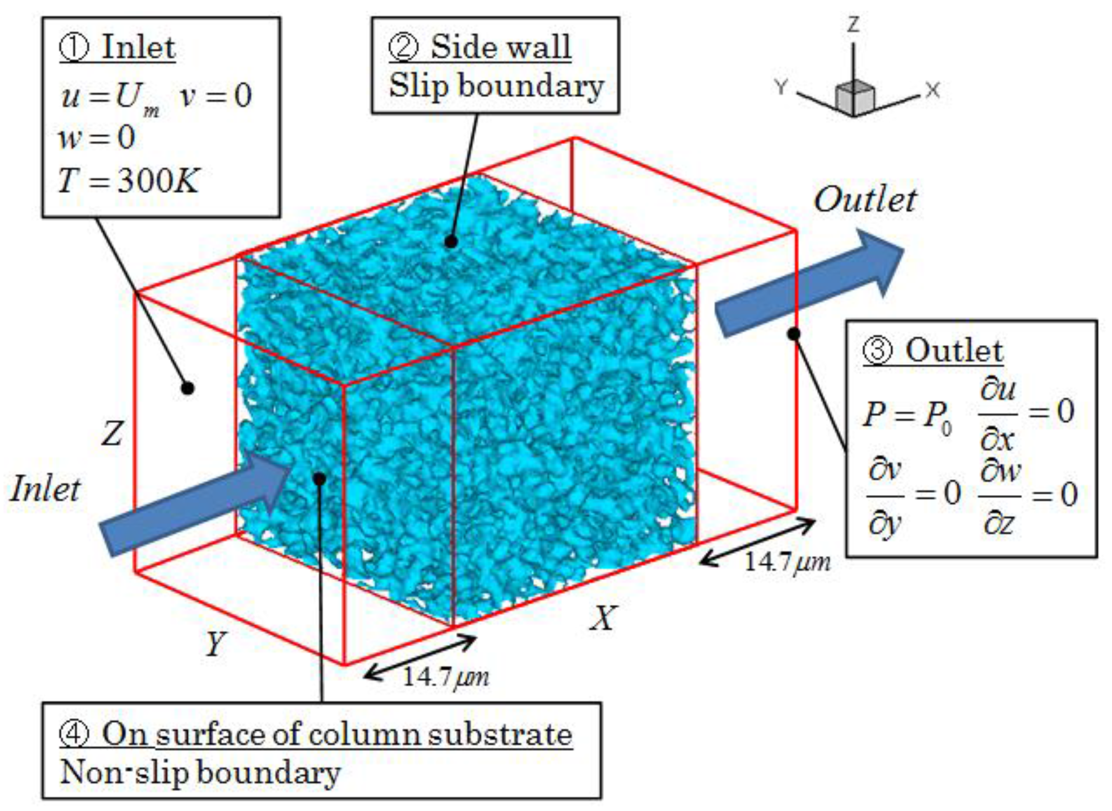
In the simulation, a D3Q15 model was used to perform a three-dimensional calculation [4,5,6,7,8]. In this model, the space discretization was achieved using square lattices. The flow was calculated based on the distribution function for pressure, p. As shown in Figure 1, the three-dimensional structure of the monolithic column was used in the simulation. Figure 2 shows the numerical domain. In this figure, the X-axis represents the flow direction, the Y-axis represents the horizontal direction, and the Z-axis represents the height direction. The porous structure of the monolithic filters obtained by the X-ray CT was placed at the center of the numerical domain. Its size was 128 μm × 98 μm × 98 μm, and the number of lattices was 261 × 201 × 201. The spatial grid of δx was 0.49 μm, corresponding to the exact spatial resolution in the X-ray CT measurement. The monolithic column was placed in the range of 15 μm < X < 113 μm.
The boundary conditions were as follows: (1) an inflow boundary was adopted for the inlet [9]; (2) a slip boundary was adopted for the top, bottom, right, and left walls (symmetric planes); (3) a free outflow boundary was adopted for the outlet; and (4) a non-slip boundary was adopted on the surface of the column substrate. Water was used as the fluid, and the flow rate was 1 mm/s.
3. Results and Discussion
3.1. Flow Field
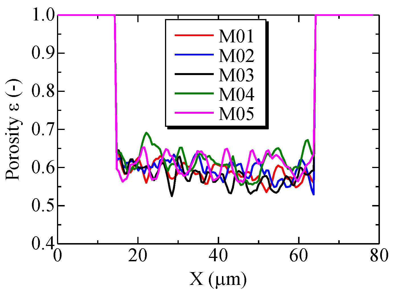
Figure 3 shows the distribution of porosity (ε) of M01–M05, which indicates the change in the porosity along the flow direction when the size of the monolithic column was W = 49 μm; the porosity is expressed in the form of the average value on the Y-Z plane. The distribution of the porosity was almost uniform inside the monolithic column, although the porosity slightly varied.
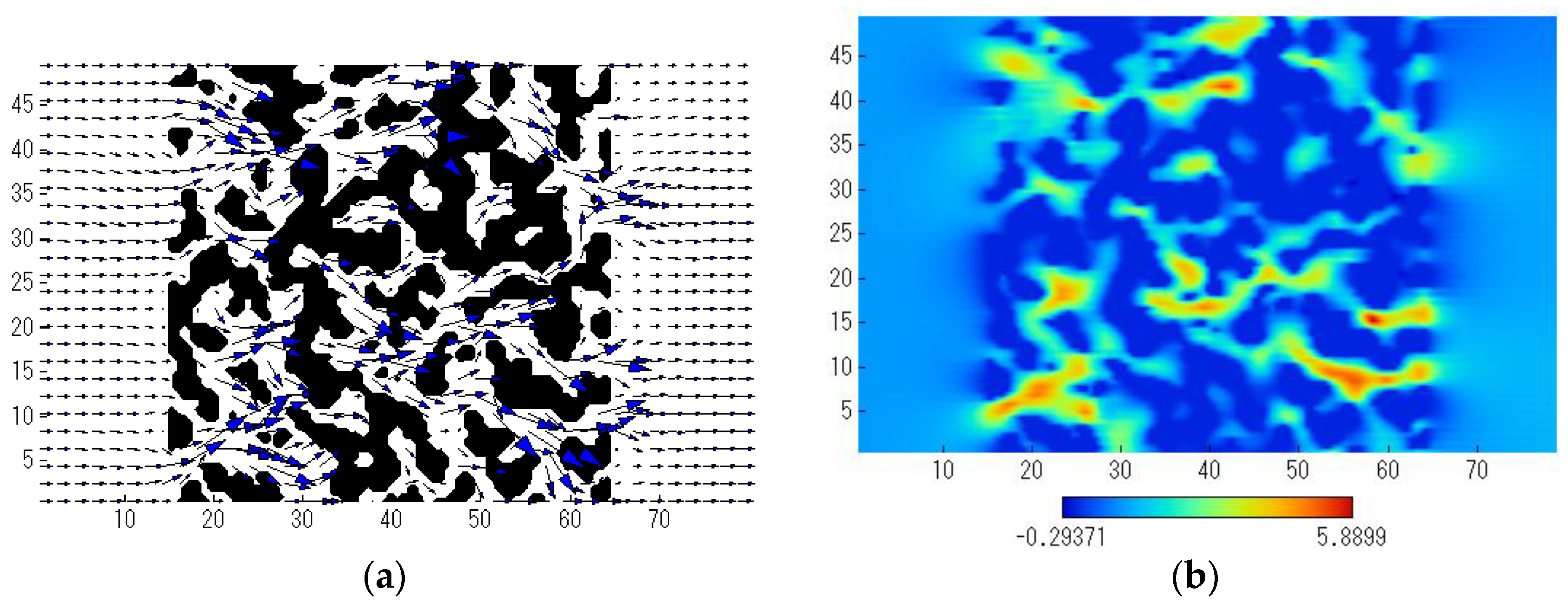
Next, the flow field in the monolithic column is discussed. Figure 4, Figure 5, Figure 6, Figure 7 and Figure 8 show the two-dimensional distribution of flows on the X-Y plane at Z = 25 μm when each monolithic width of W = 49 μm was used. One is the internal structure of the monolithic column with the velocity vector, and the other is the distribution of the velocity along the X direction. As shown in Table 1, the porosity and the pore size for each monolith are different. Although the flow velocity at the inlet was 1 mm/s, it increased to approximately 8 mm/s at the maximum when the flow passed through a narrow part in the column substrate of M02. For all cases, there was a region where the flow recirculation occurred because the velocity in the X direction was negative. The distributions of the pores were not locally uniform, and the velocity and the direction of the flow greatly varied. The maximum value of the velocity was different. However, it is difficult to discuss the difference between these flow fields quantitatively. Then, the pressure distributions were compared.
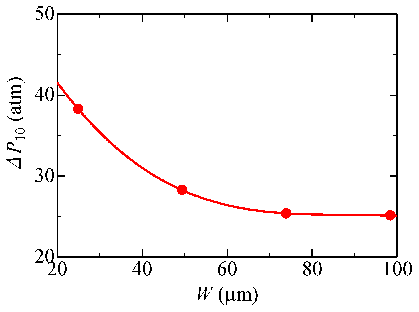
The pressure distribution in each monolithic column was investigated and the pressure drop was compared among the five monolithic columns. Preliminary, it was found that the pressure drop varied according to the numerical size of the column. The reason for this is when the height (width) of the numerical domain is extremely small, the channel where the flow can pass through the column is considerably limited. Therefore, the size of W must be sufficiently large. Then, the pressure drop, ΔP10, which corresponded to a column length of 10 cm, was obtained and the flow was calculated with different sizes of W. Figure 9 shows the numerical results obtained when W = 24.5, 49.0, 73.5, and 98.0 μm. As shown in this figure, the pressure drop decreased as W increased. Moreover, when W = 49 μm, the flow converged to a certain value. According to the results obtained in previous experiments, the pressure loss was approximately 30 atm [1] when the column length was 10 cm. Since this value was close to the convergence value obtained in the simulation shown in Figure 9, the present results were considered reasonable.
The pressure distributions of the five monolithic columns when W = 49 μm were compared, and they are shown in Figure 10. It is seen that the pressure in each column decreased at an almost constant inclination. The pressures at the inlets greatly differed from each other. In other words, the difference in pressure (pressure drop) before and after the column differed according to the column. The order of the magnitudes of the pressure drop was M03 > M01 > M02 > M05 > M04. Therefore, the value of the pressure drop differed according to the column. Then, the values of the porosity shown in Table 1 were noticed. Since the order of the values of the porosity was M03 < M01 < M02 < M05 < M04, the pressure drop decreased as the porosity increased. This could be because the ratio of the space used for the flow channel was decreased when the porosity was low, resulting in an increase of flow resistance.
To confirm the above discussion, the relationship between the average porosity and the pressure drop in the monolithic column was investigated. The results are shown in Figure 11. The pressure drop was smaller in the column with the higher porosity. However, although the porosity of M01 was almost the same as that of M03, the pressure drop greatly differed between these two columns. Regarding the other three columns, although the porosity differed between them to some extent, the difference in the pressure drop was small. Therefore, factors other than the porosity, which could affect the pressure drop, must be taken into consideration. Expectedly, as the pore size was larger in the monolithic column, more space was available for the flow. Then, the pore size (the average pore diameter) in Table 1 was examined. In general, the surface area (wetted area) of the column substrate increases as the pore diameter decreases. Therefore, the pressure drop is predicted to increase as the pore diameter decreases [10]. The order of the average pore size in Table 1 was M03 < M02 < M01 < M05 < M04. Since the difference in the average pore size between M01 and M03 was particularly large, it was suggested that the effects of both the porosity and the pore size could explain the order of the magnitudes of the pressure drop. Therefore, both the porosity and the pore size must be considered for the pressure drop in the column substrate. It was revealed that the pressure drop decreased as the porosity and/or the pore size increased.
3.2. Channel Length
To study the flow field further, the channel length of the flow was evaluated. Particles were added to the fluid. Here, the channel length corresponded to the length of the trajectory of the particle in the flow from the inlet to the outlet of the column. The magnitude of the pressure drop in each column was examined by comparing the channel length. The density of particles was set to be the same as that of the fluid, and the particle diameter was 200 nm. Particles were equally allocated to lattice points at the inlet of the numerical domain. The formula that expresses the flow of particles is shown below.
In this formula, ρp represents the density of particles, dp represents the particle diameter, CD represents the drag coefficient, V and u represent the velocity vector of the particle and the flow, respectively [11]. As already explained, we set the particle density to be equal to that of the fluids (water). Also, the velocity of the particle at the inlet was the same value as the inflow velocity. Then, the particle followed the fluid flow stream. It was confirmed that the flow path length did not change when the particle diameter was below 200 nm. Figure 12 shows the obtained channel length, L. The width (thickness) of the monolithic column was 49 μm. As shown in this figure, the channel length differed slightly according to the column. However, the difference was as small as approximately 1 μm, and the channel length was approximately 1.2 times larger than the thickness of the column. Therefore, the channel length was almost constant regardless of the type of column, and the effect of the channel length on the pressure drop was revealed to be small.
3.3. Velocity Distribution
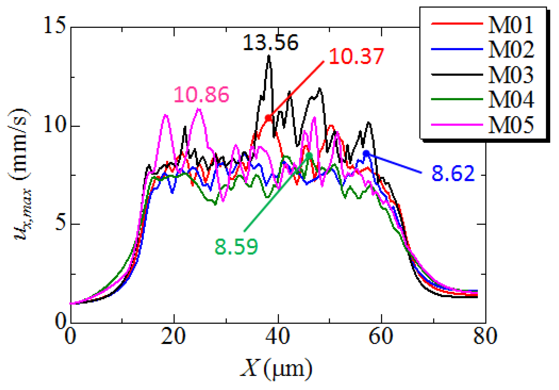
It was found that the porosity and the average pore size differed according to the column. These two factors surely affect the flow in the column. To examine the differences in the pressure drop among the five columns, the flow velocity passing through each column was compared and discussed. Based on Figure 4, Figure 5, Figure 6, Figure 7 and Figure 8, it was found that the flow was locally accelerated due to the narrow space between substrates. If the flow is smooth, the pressure drop could be small. Then, the maximum value of the flow velocity was examined. Figure 13 shows the maximum velocity in the X direction measured on each Y-Z plane in the numerical domain. The maximum velocity observed inside the monolith column is shown in this figure. The value in M03 which exhibited the maximum pressure drop was 13.56 mm/s, and this value was clearly larger than those in the other columns. However, even in M03 there was a region where the flow velocity was locally smaller than that in the other columns. In M04, where the pressure drop was the smallest, the maximum flow velocity was only 8.59 mm/s. As shown in Figure 4, Figure 5, Figure 6, Figure 7 and Figure 8, when a locally occluded region existed in the column, the region with an extremely large flow velocity was observed. Therefore, if the flow is smooth in the column, the pressure drop is smaller.
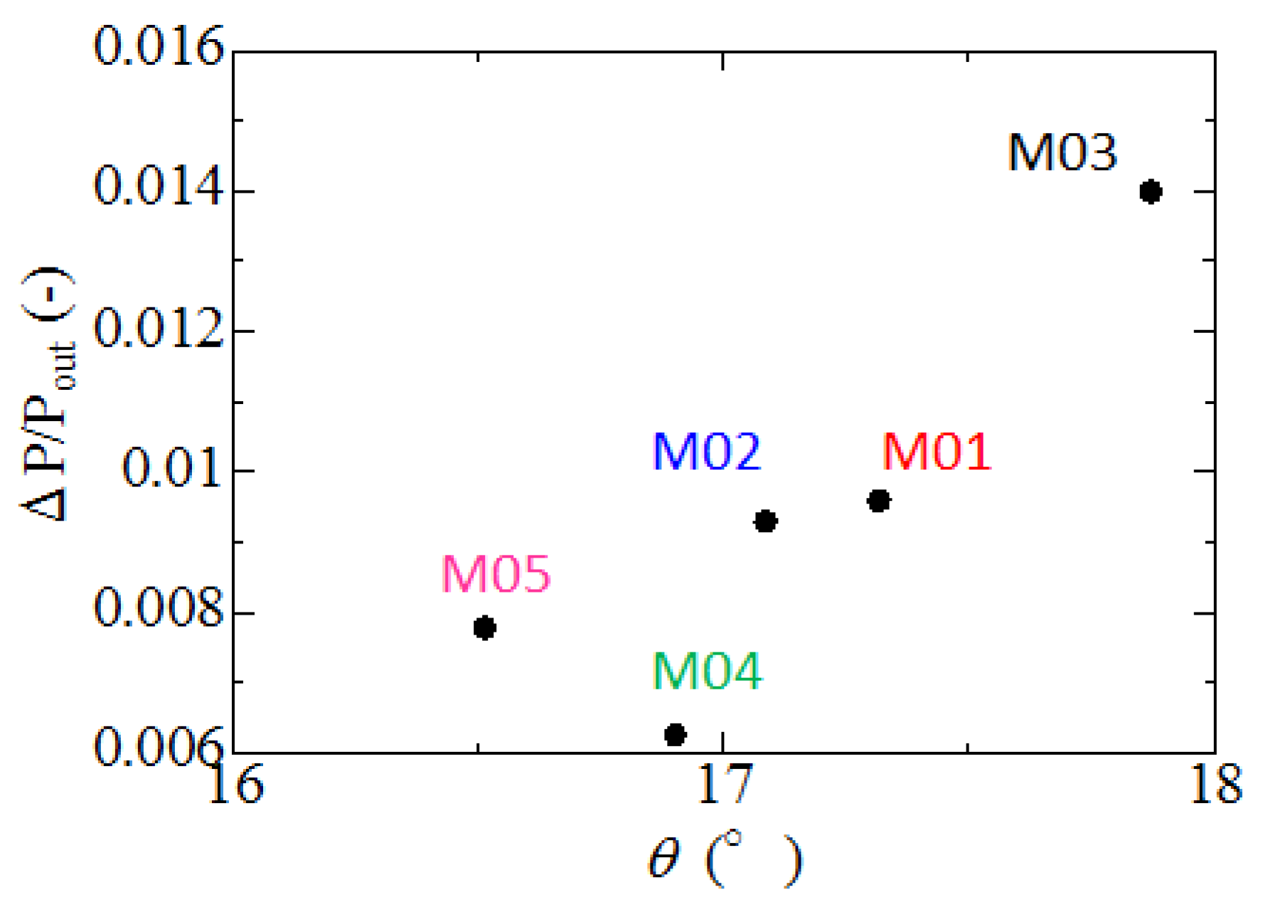
Next, the flow direction in the column was further examined. Needless to say, the more complex structure the monolith column has, the higher the pressure drop could be. Here, the angle (displacement angle θ) between the velocity vector of the flow at each lattice point and the X-axis (direction of the main flow) was evaluated. The displacement angle θ corresponded to the angle of the flow to the X-axis. That is, we could examine the change in the flow direction due to the rough structure of the column substrate when the flow passed through the column. Figure 14 shows the relationship between the pressure drop and the average incident angle θ in monolithic columns M01–M05. As shown in this figure, the pressure drop increased with the incident angle to the main flow. Therefore, when the structure of the column substrate is more complicated, the change in the flow direction becomes larger, resulting in a larger pressure drop.
4. Conclusions
Using five types of monolithic columns formed in different conditions, the numerical simulation of fluids in the monolith column was presented. Since the pressure drop differed according to the structure of each monolithic column, the discussion on the main factor of the pressure drop was conducted by analyzing the flow in the column in detail. The obtained results were summarized as follows:
- (a)
- When the height (width) of the numerical domain was 49 μm or greater, the pressure drop was saturated. The order of the magnitudes of the pressure drop was M03 > M01 > M02 > M05 > M04. The pressure drop was smaller as the porosity and/or the pore size increased.
- (b)
- When particles were added to the flow, the trajectory of each particle was examined in order to evaluate the flow path length. Consequently, the flow path length was almost constant regardless of the column type, and was approximately 1.2 times larger than the thickness of the column.
- (c)
- The maximum flow velocity in the X direction increased with the pressure drop. The change in the flow direction was larger as the pressure drop increased. As a result, when the structure of the column substrate was more complicated, the change in the flow direction became larger, resulting in the larger pressure drop.
Acknowledgments
The authors thank Tomonari Umemura of the Tokyo University of Pharmacy and Life Sciences for helpful discussions.
Author Contributions
Kazuhiro Yamamoto had the original idea for the study, and drafted the manuscript. Yuuta Tajima was responsible for data analyses in the simulation. All authors read and approved the final manuscript.
Conflicts of Interest
The authors declare no conflict of interest.
References
- Umemura, T.; Kamiya, S.; Itoh, A.; Chiba, K.; Haraguchi, H. Preparation and characterization of methacrylate-based semi-micro monoliths for high-throughput bioanalysis. Anal. Bioanal. Chem. 2006, 386, 566–571. [Google Scholar] [CrossRef] [PubMed]
- Shu, S.; Kobayashi, H.; Kojima, N.; Sabarudin, A.; Umemura, T. Preparation and characterization of lauryl methacrylate-based monolithic microbore column for reversed-phase liquid chromatography. J. Chromatogr. A 2011, 1218, 5228–5234. [Google Scholar] [CrossRef] [PubMed]
- Chen, S.; Doolen, G.D. Lattice Boltzmann method for fluid flows. Ann. Rev. Fluid Mech. 1998, 30, 329–364. [Google Scholar] [CrossRef]
- Yamamoto, K.; Komiyama, R.; Umemura, T. Numerical simulation on flow in column chromatography. Int. J. Mod. Phys. C 2014, 24, 1–7. [Google Scholar] [CrossRef]
- Yamamoto, K.; Satake, S.; Yamashita, H.; Takada, N.; Misawa, M. Lattice Boltzmann simulation on flow with soot accumulation in diesel particulate filter. Int. J. Mod. Phys. C 2007, 18, 528–535. [Google Scholar] [CrossRef]
- Yamamoto, K.; Satake, S.; Yamashita, H.; Takada, N.; Misawa, M. Fluid simulation and X-ray CT images for soot deposition in a diesel filter. Eur. Phys. J. 2009, 171, 205–212. [Google Scholar] [CrossRef]
- Yamamoto, K.; Yamauchi, K.; Takada, N.; Misawa, M.; Furutani, H.; Shinozaki, O. Lattice Boltzmann simulation on continuously regenerating diesel filter. Philos. Trans. A R. Soc. Lond. 2011, 369, 2584–2591. [Google Scholar] [CrossRef] [PubMed]
- Yamamoto, K.; Matsui, K. Diesel exhaust after-treatment by silicon carbide fiber filter. Fibers 2014, 2, 128–141. [Google Scholar] [CrossRef]
- Zou, Q.; He, X. On pressure and velocity boundary conditions for the lattice Boltzmann BGK model. Phys. Fluids 1997, 9, 1591–1598. [Google Scholar] [CrossRef]
- Bird, R.B.; Stewart, W.E.; Lightfoot, E.N. Interphase transport in isothermal systems. In Transport Phenomena, 2nd ed.; Wiley: New York, NY, USA, 1960. [Google Scholar]
- Imai, Y.; Miki, T.; Ishikawa, T.; Aoki, T.; Yamauchi, T. Deposition of micrometer particles in pulmonary airways during inhalation and breath holding. J. Biomech. 2012, 45, 1809–1815. [Google Scholar] [CrossRef] [PubMed]
- Wang, Y.; Meng, L.; Pittman, E.N.; Etheredge, A.; Hubbard, K.; Trinidad, D.A.; Kato, K.; Ye, X.; Calafat, A.M. Quantification of urinary mono-hydroxylated metabolites of polycyclic aromatic hydrocarbons by on-line solid phase extraction-high performance liquid chromatography-tandem mass spectrometry. Anal. Bioanal. Chem. 2016. [Google Scholar] [CrossRef] [PubMed]
Figure 1.
Inner structure of the monolithic column of M03; (a) slice image; (b) three-dimensional structure.
Figure 1.
Inner structure of the monolithic column of M03; (a) slice image; (b) three-dimensional structure.
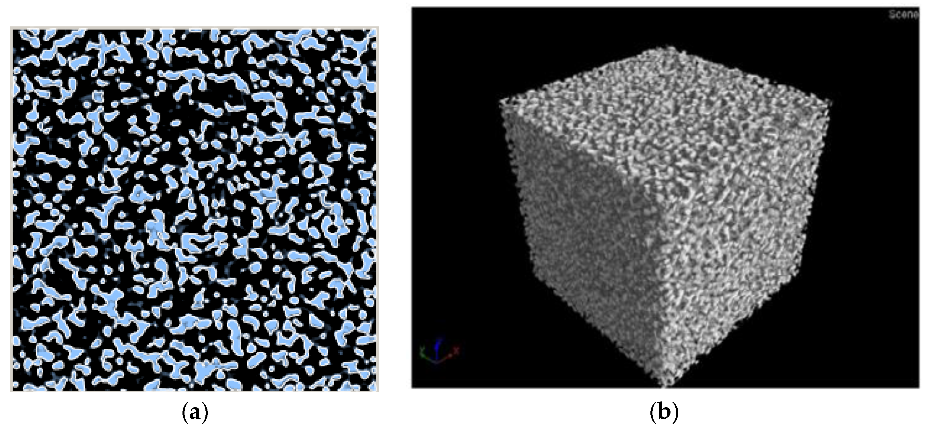
Figure 2.
Numerical domain and boundary conditions are shown.

Figure 3.
Distributions of average porosity in Y-Z plane.

Figure 4.
(a) Monolith structure of M01 with velocity vector in X-Y plane; (b) velocity in X direction.
Figure 4.
(a) Monolith structure of M01 with velocity vector in X-Y plane; (b) velocity in X direction.

Figure 5.
(a) Monolith structure of M02 with velocity vector in X-Y plane; (b) velocity in X direction.
Figure 5.
(a) Monolith structure of M02 with velocity vector in X-Y plane; (b) velocity in X direction.
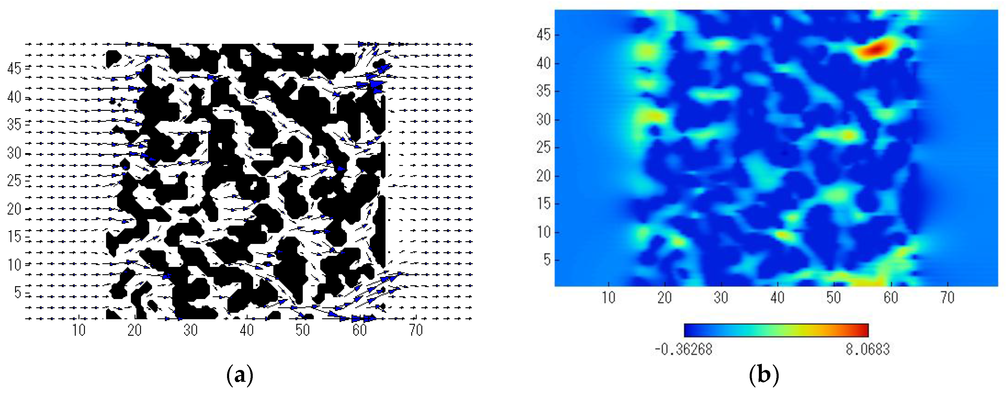
Figure 6.
(a) Monolith structure of M03 with velocity vector in X-Y plane; (b) velocity in X direction.
Figure 6.
(a) Monolith structure of M03 with velocity vector in X-Y plane; (b) velocity in X direction.
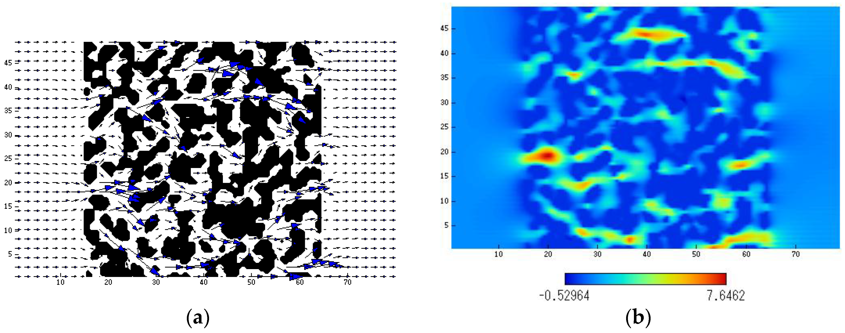
Figure 7.
(a) Monolith structure of M04 with velocity vector in X-Y plane; (b) velocity in X direction.
Figure 7.
(a) Monolith structure of M04 with velocity vector in X-Y plane; (b) velocity in X direction.
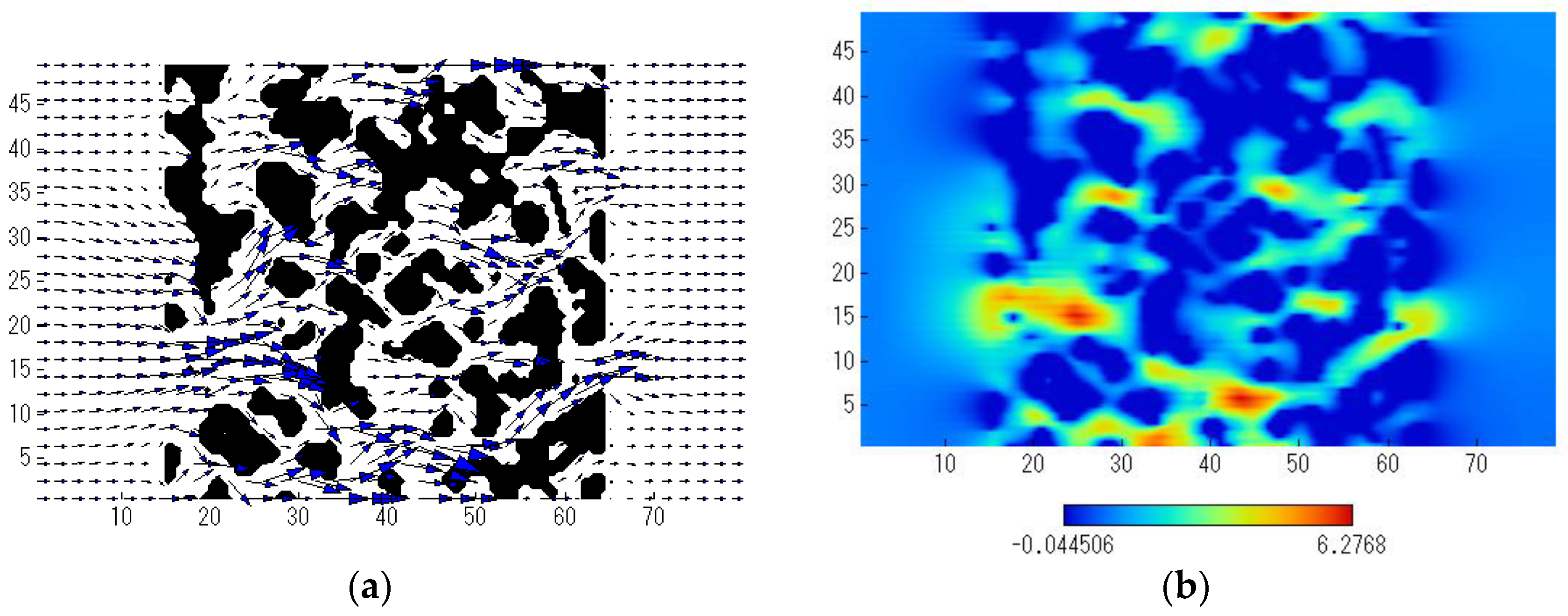
Figure 8.
(a) Monolith structure of M05 with velocity vector in X-Y plane; (b) velocity in X direction.
Figure 8.
(a) Monolith structure of M05 with velocity vector in X-Y plane; (b) velocity in X direction.
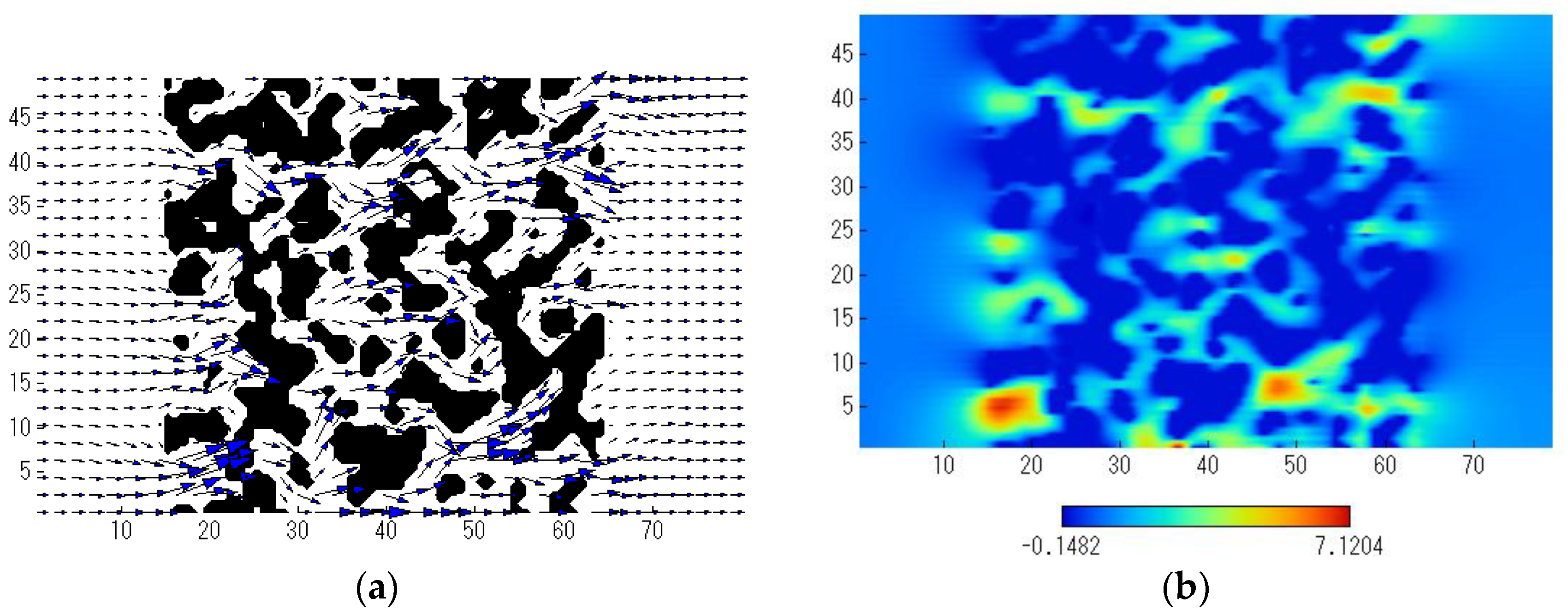
Figure 9.
Pressure drop of 10 cm monolith at different widths of W.

Figure 10.
Pressure distribution of monolith column from M01 to M05.
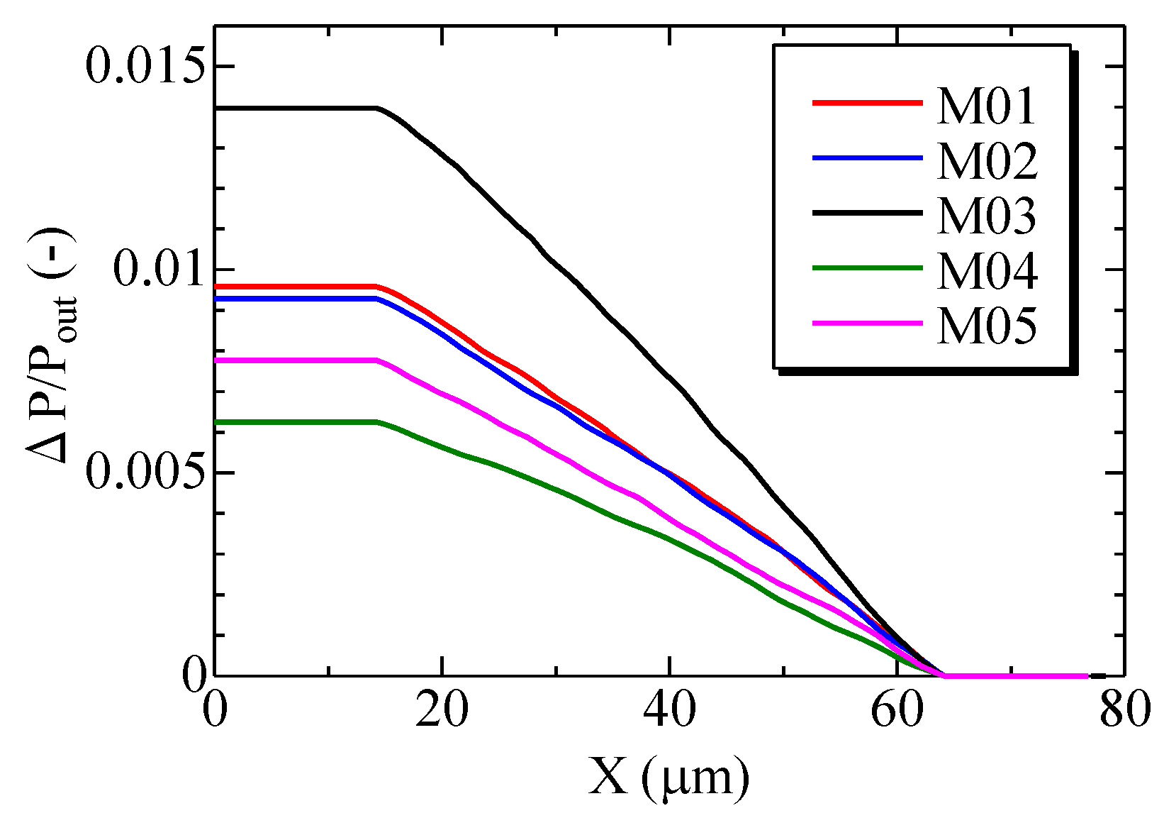
Figure 11.
Variation of pressure drop with mean porosity.
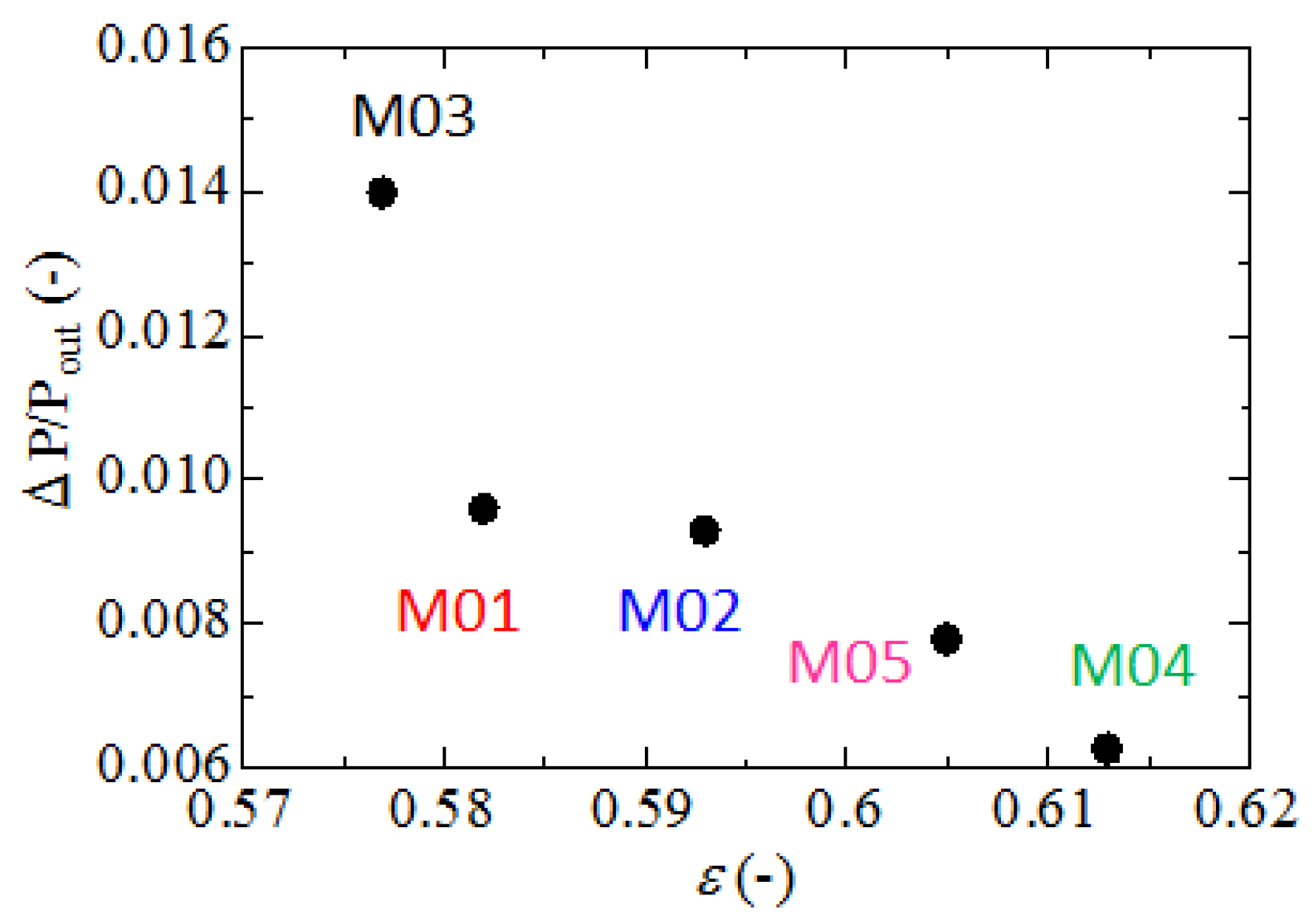
Figure 12.
Flow path length in monolithic column.
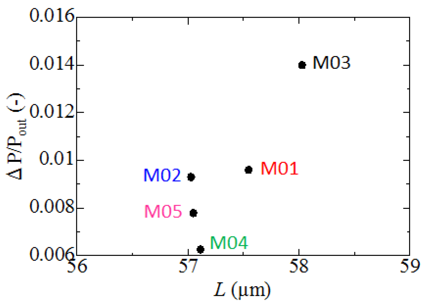
Figure 13.
Maximum velocity along the flow direction.

Figure 14.
Displacement angle against the flow direction.


| No. | Ratio of Cross-Linker | Reactor Vessel for Polymerization Reaction | Reaction Temperature | Porosity ε | Pore Size Dp |
|---|---|---|---|---|---|
| M01 | 10% | SUS a pipe | 60 °C | 0.582 | 4.43 μm |
| M02 | 25% | SUS a pipe | 60 °C | 0.593 | 4.28 μm |
| M03 | 10% | SUS a pipe | 90 °C | 0.577 | 4.01 μm |
| M04 | 10% | PEEK b tube | 60 °C | 0.613 | 4.65 μm |
| M05 | 10% | PEEK b tube | 90 °C | 0.605 | 4.56 μm |
a Steel use stainless; b Polyether ether ketone.
© 2017 by the authors. Licensee MDPI, Basel, Switzerland. This article is an open access article distributed under the terms and conditions of the Creative Commons Attribution (CC BY) license ( http://creativecommons.org/licenses/by/4.0/).
Share and Cite
MDPI and ACS Style
Yamamoto, K.; Tajima, Y. Numerical Simulation of Fluid Dynamics in a Monolithic Column. Separations 2017, 4, 3. https://doi.org/10.3390/separations4010003
AMA Style
Yamamoto K, Tajima Y. Numerical Simulation of Fluid Dynamics in a Monolithic Column. Separations. 2017; 4(1):3. https://doi.org/10.3390/separations4010003
Chicago/Turabian StyleYamamoto, Kazuhiro, and Yuuta Tajima. 2017. "Numerical Simulation of Fluid Dynamics in a Monolithic Column" Separations 4, no. 1: 3. https://doi.org/10.3390/separations4010003
Note that from the first issue of 2016, this journal uses article numbers instead of page numbers. See further details here.