Article

On the Bias of the Maximum Likelihood Estimators of Parameters of the Weibull Distribution

Department of Mathematics, School of Science, Beijing Jiaotong University, Beijing 100044, China
*
Author to whom correspondence should be addressed.
Math. Comput. Appl. 2017, 22(1), 19; https://doi.org/10.3390/mca22010019
Submission received: 18 September 2016 / Accepted: 20 January 2017 / Published: 15 February 2017

Abstract

:
Usually, the parameters of a Weibull distribution are estimated by maximum likelihood estimation. To reduce the biases of the maximum likelihood estimators (MLEs) of two-parameter Weibull distributions, we propose analytic bias-corrected MLEs. Two other common estimators of Weibull distributions, least-squares estimators and percentiles estimators, are also introduced. Based on a comparison of their performances in the simulation study, we strongly recommend the analytic bias-corrected MLEs for the parameters of Weibull distributions, especially when the sample size is small.

1. Introduction

We investigate several different estimations of the parameters of the two-parameter Weibull distribution, and analyze two different methods to reduce the biases of maximum likelihood estimators (MLEs).
The following formula is the cumulative distribution function of a Weibull distribution:
F ( x ; k , λ ) = 1 e ( x λ ) k , x > 0 , λ > 0 , k > 0 0 x 0 ,
and its probability density function is:
f ( x ; k , λ ) = ( 1 λ ) k k x k 1 e ( x λ ) k , x > 0 , λ > 0 , k > 0 0 x 0 ,
The Weibull distribution was first identified by Fréchet in 1927, and it was named after Waloddi Weibull, a Swedish mathematician who described this distribution in detail in 1951. Rammler [1] used it to explain a particle size distribution.
The Weibull distribution is not a single distribution, but is in fact a family of distributions, because of the distribution having the shape parameter. The shape parameter enables Weibull distributions to take on various shapes, contingent on the value of the shape parameter. Those distributions are particularly useful in modeling applications since they are flexible enough to model various datasets.
The Weibull distribution has a relatively simple form. Nevertheless, the shape parameter enables the Weibull to assume a variety of shapes. This combination of simplicity and flexibility in the shape of the Weibull distribution makes it an effective distributional model in reliability applications. The ability to model various distributional shapes by using a relatively simple distributional form is possible with many other distributional families, as well.
The Weibull distribution is associated with various other distributions. For instance, it is well known that a Weibull distribution contains the exponential distribution (when k = 1 ) and the Rayleigh distribution (when k = 2 ). Recently, Ling and Giles [2] studied the Rayleigh distribution and the bias adjustment of the Rayleigh distribution. The Weibull distribution is a special condition of the generalized extreme value distribution, which was proposed by Fréchet [3]. This closely-related Fréchet distribution has the probability density function:
f F r e c h e t ( x ; k , λ ) = k λ ( x λ ) 1 k e ( x λ ) k x > 0 , λ > 0 , k > 0 0 x 0 . ,
Actually, f F r e c h e t ( x ; k , λ ) = f W e i b u l l ( x ; k , λ ) . A Weibull distribution is also characterized in terms of a uniform distribution; when U is uniformly distributed on ( 0 , 1 ) , then the random variable λ ( ln ( U ) ) 1 / k is Weibull distributed with parameters k and λ.
The Weibull distribution has been used in numerous fields, such as production, industry, data analysis, reliability in devices, materials testing and environmental assessment. This distribution was studied and used in an aircraft system to investigate operational reliability by Kaltschmidt et al. [4]. Nikolaj [5] showed that this distribution can be used in oil pollution examination. Singh [6] studied the Weibull distribution and worked in hydrology by using this distribution. Aarset [7] applied a Weibull distribution to test failure times of devices, and the data were further analyzed and modified by Lai et al. [8]. It was used in breakdown voltage estimation by Hirose [9], and Fabiani [10] used it to test electrical breakdown of insulating materials. It was applied to censored data by Ghitany et al. [11]. In the study of wind energy, the Weibull distribution was also applied by Akdaǧ et al. [12].
Additionally, we have also considered the exponential distribution. When the value of k is one, the Weibull distribution becomes the exponential distribution, which is studied widely. The cumulative distribution function of the exponential distribution is:
F ( x ; k , λ ) = 1 e λ x , x > 0 , λ > 0 0 x 0 ,
and its probability density is:
f ( x ; k , λ ) = λ e λ x , x > 0 , λ > 0 0 x 0 ,
Maximum-likelihood estimators of the Weibull distribution are commonly used. However, they are biased, and thus, in this paper, we propose analytic bias-corrected MLEs for the two-parameter Weibull distribution. The analytic bias-corrected MLEs are considered in Section 2 and compared with the other bias-corrected MLEs, which are also known as bootstrap bias-corrected MLEs. In Section 3 and Section 4, we introduce two other commonly-used estimators. Monte Carlo experiments are conducted for the simulation study. Tabular and graphical representations of the results are presented in this section. The results indicate that the analytic bias-corrected estimators are superior to not only traditional bootstrap bias-corrected estimators, but also the other two commonly-used estimators. Thus, the analytic bias-corrected estimators should be highly recommended. Finally, we apply these estimators to an actual situation and draw conclusions.

2. Maximum Likelihood Estimators and Different Bias-Corrected Maximum Likelihood Estimators

2.1. Maximum Likelihood Estimators

Suppose the sample ( x 1 , x 2 , . . . x n ) is generated from the log–normal distribution. The likelihood function of the Weibull distribution is:
L = ( 1 λ ) k n k n ( i = 1 n x i ) k 1 e λ k i = 1 n x i k
and the formula for the log-likelihood function is:
l = log L = k n log λ + n log k + ( k 1 ) i = 1 n log x i λ k i = 1 n x i k
The MLEs can be obtained by solving the following equations:
l λ = k n λ + k λ k 1 i = 1 n x i k = 0    
l k = n log λ + n k + i = 1 n log x i λ k i = 1 n x i k log x i + λ k ( log λ ) i = 1 n x i k = 0
The Newton-Raphson method is used to solve these two equations, and solutions k ^ and λ ^ were obtained.

2.2. Analytic Bias-Corrected Maximum Likelihood Estimators

Suppose l(σ) is the log-likelihood function of the Weibull distribution based on a sample size n. The joint cumulants of the derivatives of the log-likelihood function are:
h i j = E [ 2 l σ i σ j ] , i , j = 1 , 2 , . . . , q
h i j m = E [ 3 l σ i σ j σ m ] , i , j , m = 1 , 2 , . . . , q
h i j , m = E [ 2 l σ i σ j l σ m ] , i , j , m = 1 , 2 , . . . , q
h i j ( m ) = h i j σ m , i , j , l = 1 , 2 , . . . , q
In this part, the function l(σ) is regular with respect to all derivatives up to the third order.
We assume that Equations (10)–(13) are O ( n ) . Cox and Snell [13] showed that for sample data that are independent, but not always identically distributed, the bias of the s-th element of the MLE of σ is:
B i a s ( σ ^ s ) = i = 1 q j = 1 q l = 1 q h s i h s j [ ( 1 / 2 ) h i j m + h i j , m ] + O ( n 2 ) , i , j , m = 1 , 2 , . . . , q
where h i j is the ( i , j ) -th element of the inverse of Fisher’s information matrix, H = { h i j } . Cordeiro and Klein [14] observed that the bias expression still holds even if the observations are non-independent, proved that all of the h terms are O ( n ) and recommended another form for the expression:
B i a s ( σ ^ s ) = i = 1 q h s i j = 1 q l = 1 q h s j [ h i j m ( 1 / 2 ) h i j m ] h j m + O ( n 2 ) , i , j , m = 1 , 2 , . . . , q
In Equation (15), we define:
a i j ( m ) = h i j ( m ) 1 2 h i j m , i , j , m = 1 , 2 , . . . , q
and (15) can be written as:
B i a s ( σ ^ ) = H 1 A v e c ( H 1 ) + O ( n 2 )
where v e c ( H 1 ) is a transformation of the matrix H 1 into a vector form, and the matrix A is:
A ( m ) = { a i j ( m ) } ; i , j , m = 1 , 2 , . . . , q
A = [ A ( 1 ) A ( 2 ) . . . A ( q ) ]
Then, the bias-corrected MLEs are:
B i a s λ ˜ a n a l y t i c c o r r e c t e d k ˜ a n a l y t i c c o r r e c t e d = σ ^ H ^ 1 A ^ v e c ( H ^ 1 )
where H ^ = ( H ) | σ ^ and A ^ = ( A ) | σ ^ . The bias of σ ˜ can be proven to be O ( n 2 ) . The values of the elements of σ ^ can be obtained based on the maximum likelihood equations.
This method was applied to the generalized Pareto distribution by Giles et al. [15] successfully, and Min Wang [16] used it for the weighted Lindley distribution with Wentao Wang.
Specific calculation procedures of the bias-corrected MLEs of the parameters of the Weibull distribution are listed in Appendix A.

2.3. Bootstrap Bias-Corrected Estimators

In this section, the bootstrap bias-corrected estimators of the Weibull distribution are considered, which were suggested by Mackinnon and Smith [17].
The solutions k ^ and λ ^ are the particular values of estimators based on MLEs, and we regard k ^ and λ ^ as the particular parameters of the log–normal distribution, from which the N B replicative samples are generated. Thus, the corresponding estimates ( k ^ 1 , k ^ 2 , . . . , k ^ n ) and ( λ ^ 1 , λ ^ 2 , . . . , λ ^ n ) are obtained.
The bootstrap bias-corrected parameters are k ˇ = 2 k ^ ( 1 / N B ) j = 1 N B k ^ j , λ ˇ = 2 λ ^ ( 1 / N B ) j = 1 N B λ ^ j (the parameters k ^ j and λ ^ j are the MLEs of k and λ from the j-th sample of the N B replication samples).
This method is fairly effective and is worth applying to various situations, which causes that many experts have investigated it. Ferrari and Cribari-Neto [18] explored the relationship between bias correction of maximum likelihood estimators through the bootstrap method, and the bootstrap method was presented by Ho and Fernandes da Silva [19] to make improvements in the MLE of Mean Time to Failure (MTTF) and p-quantiles. Focarelli [20] used the bootstrap bias-correction procedure to estimate long-run relationships from dynamic panels, with an application to money demand in the euro area.

3. Percentile Estimators

The estimators based on percentiles are also investigated. This approach was first studied by Kao [21,22] and then was explored by Mann, Schafer and Singpurwalla [23]. This method is suitable for the Weibull distribution.
Let us consider the situation where both the parameters λ and k are unknown. From the cumulative distribution function (1), we can obtain:
λ [ log ( 1 F ( x i ; k , λ ) ) ] ( 1 / k ) = x i
Suppose that ( x 1 , x 2 , . . . x n ) is a random sample of data, and the ( x ( 1 ) , x ( 2 ) , . . . x ( n ) ) is the ordered observation. Let p i be the estimate of F ( x ( i ) ; k , λ ) , then we can obtain estimates of λ and k by minimizing the equation:
i = 1 n [ x i [ log ( 1 F ( x ( i ) ; k , λ ) ) ] ( 1 / k ) ] 2
Generally, some p i ’s are used to be the estimates of the F ( x i ; k , λ ) , and the p i = ( i / ( n + 1 ) ) is most frequently used, because ( i / ( n + 1 ) ) is the expected value of F ( x ( i ) ; k , λ ) . In this article, we also use this p i .
Equation (22) is a non-linear function. To obtain estimates of the two parameters, we can solve (22) by using some non-linear regression techniques. These estimators are called percentile estimators, which were also applied and introduced by Gupta and Kundu [24].

4. Least Squares Estimators

In this section, we introduce the expressions of another estimation. This method was first applied by Swain, Venkatraman and Wilson [25] to estimate the parameters of the beta distribution, and it can be utilized in other cases, as well. Suppose that ( x 1 , x 2 , . . . , x n ) is a random sample of size n from a distribution whose distribution function is F ( x ) and that ( x ( 1 ) , x ( 2 ) , . . . , x ( n ) ) denotes the ordered set of sample observations. Jonson, Kotz and Balakrishnan [26] proposed expressions for the expectations and variances,
E ( F ( x ( i ) ) ) = i n + 1 , i = 1 , 2 , . . . , n
The least squares estimators can be obtained by minimizing:
i = 1 n [ F ( x ( i ) ) i n + 1 ] 2
We call this estimator as least squares estimator.
Therefore, in the case of the Weibull distribution, the least squares estimators of k and λ are denoted by k L s e and λ L s e , respectively. These values are obtained by minimizing:
i = 1 n [ 1 e ( x ( i ) λ ) k i n + 1 ] 2

5. Simulation Study

5.1. Procedures

In this part, the Monte Carlo experiment is described, and the simulation results are analyzed. The R 3.2.2 software [27] routines for log–normal random variates are used to generate the sample from the Weibull distribution. Then, the MLE, percentile estimation and least squares estimation can be realized by the non-linear minimization function. In the R software, the non-linear minimization function can solve a minimization problem using a Newton-type algorithm. After substituting the MLEs into the corrected formula mentioned previously, we can obtain the analytic bias-corrected estimators. The bootstrap bias-corrected estimators will be acquired after conducting the replicative MLE experiments.

5.2. Analysis of the Results

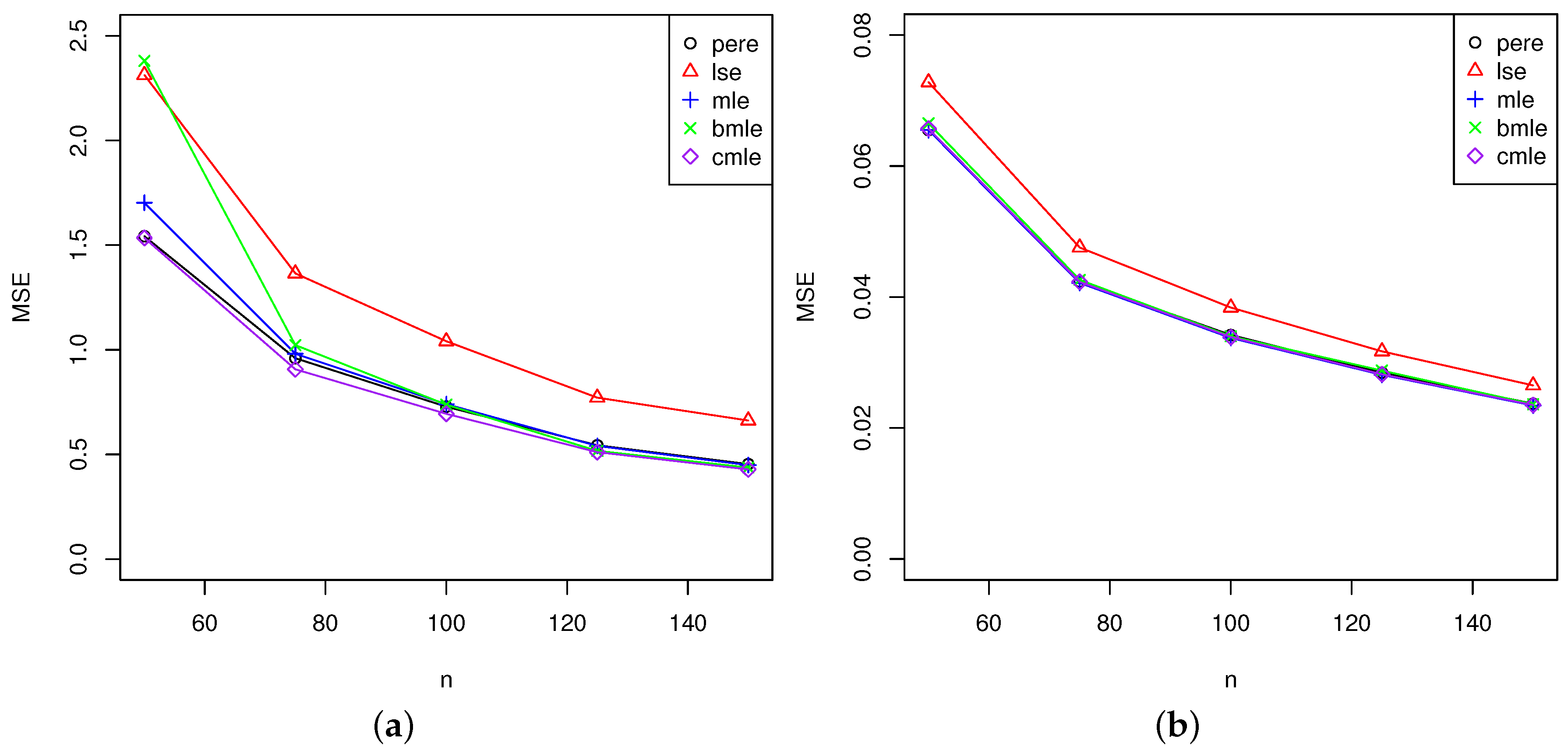
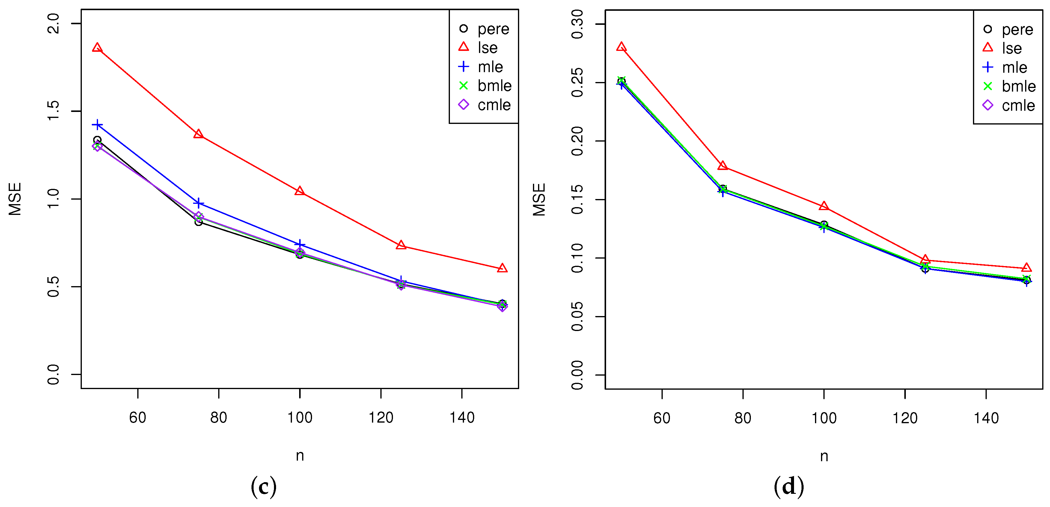
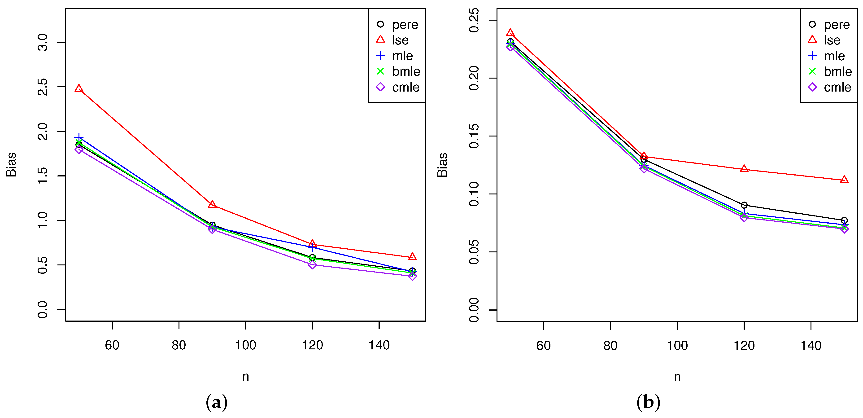
5.2.1. Comparison of Maximum Likelihood Estimators and Bias-Corrected Maximum Likelihood Estimators

Comparing the theoretical performances of the different estimators mentioned above is not convincing. Therefore, we performed extensive simulations to compare the performances of the different methods, mainly with respect to their real absolute percentage biases and percentage mean squared errors (MSEs) for different sample sizes. The percentage MSE is defined as 100 × ( MSE ( k ^ ) / k 2 ) , and the absolute percentage bias is defined as 100 × | ( mean ( k ^ ) k ) / k | .
In each section of this experiment, 20,000 Monte Carlo replications are performed, and 10,000 bootstrap samples are used for every replication.
We also investigate general Weibull distributions with some common parameter values. The exponential distribution with particular parameter value ( k = 1 ) is also investigated here. We select parameters values for the Weibull distribution ( k = 1 ) that are consistent with the data generating process being an exponential distribution.
Absolute percentage biases and MSEs of those estimators for the exponential distribution are presented in Table 1, and those for the Weibull distribution are presented in Table 2.
These tables show that the percentage biases of the analytic bias-corrected MLEs are much smaller than those of the MLEs. Meanwhile, both the analytic bias correction and bootstrap bias correction perform well. However, the Cox-Snell bias correction is more effective than the bootstrap reduction, especially with the modest sample size.
The absolute values of the percentage biases tend to decline as the sample size increases, and the percentage MSEs of the Cox-Snell estimators are smaller than those of the bootstrap estimators, except in a few cases. The MSEs and biases of the analytic bias-correction estimators are smaller than those of the other estimators.

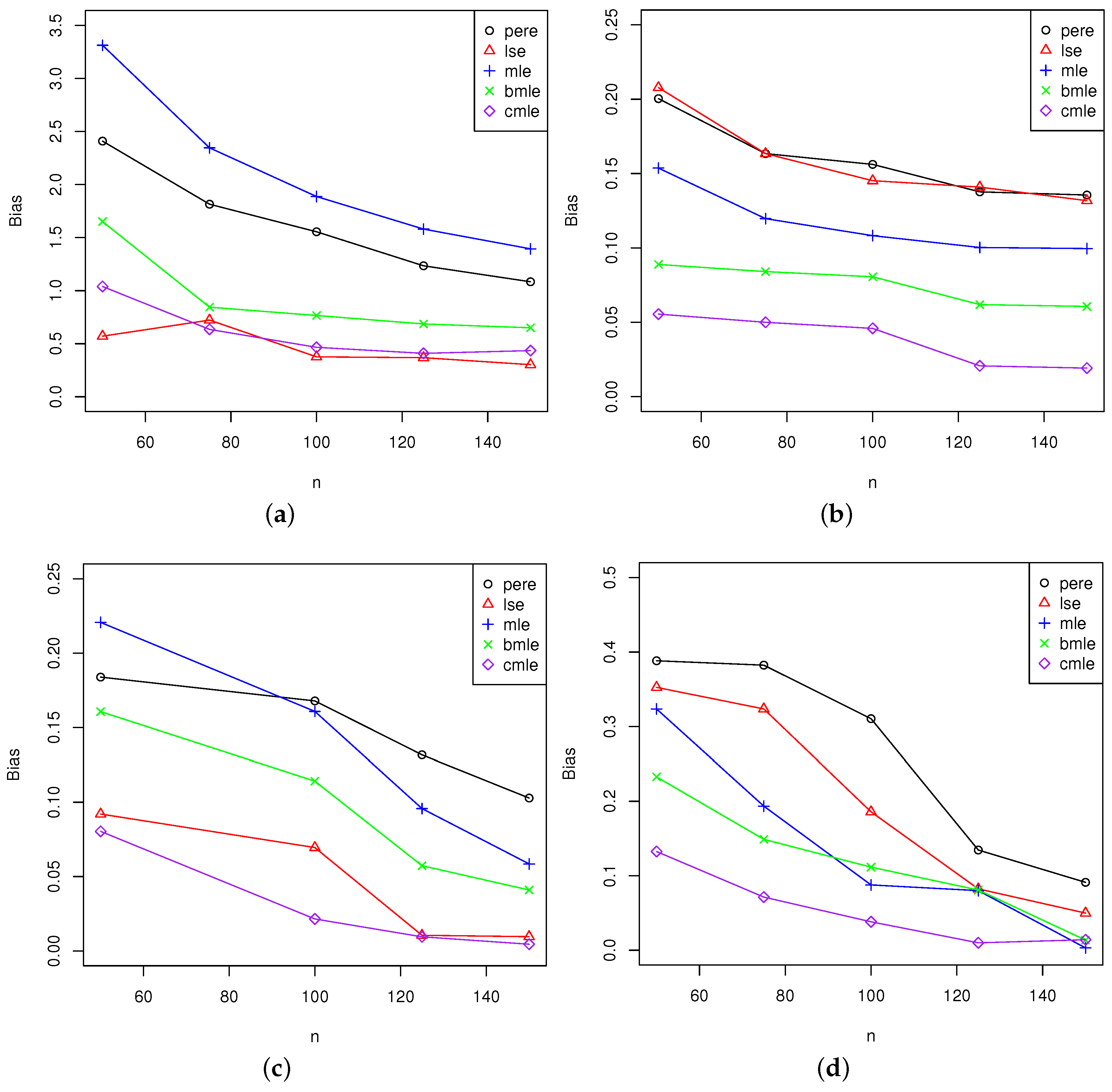
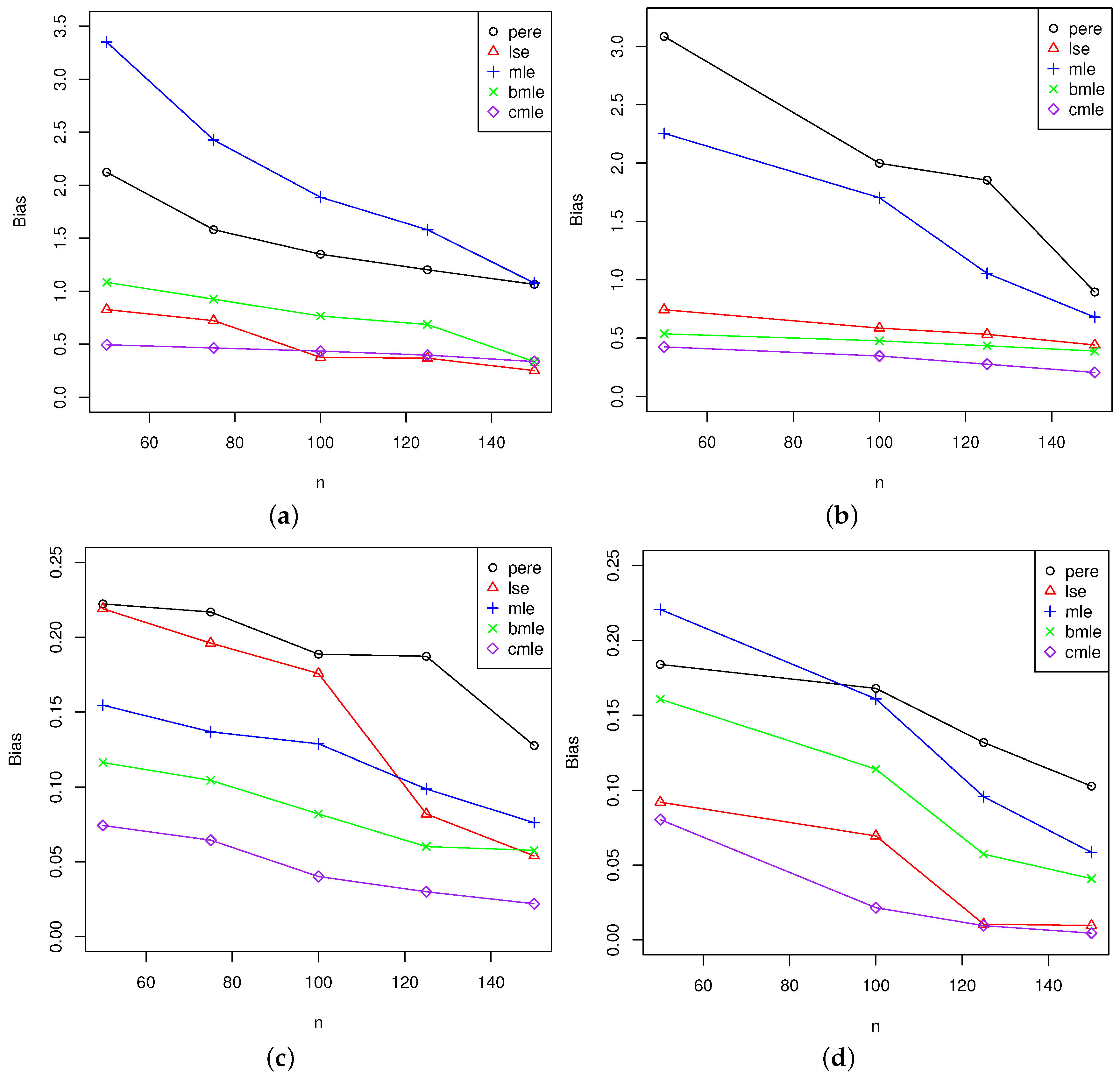
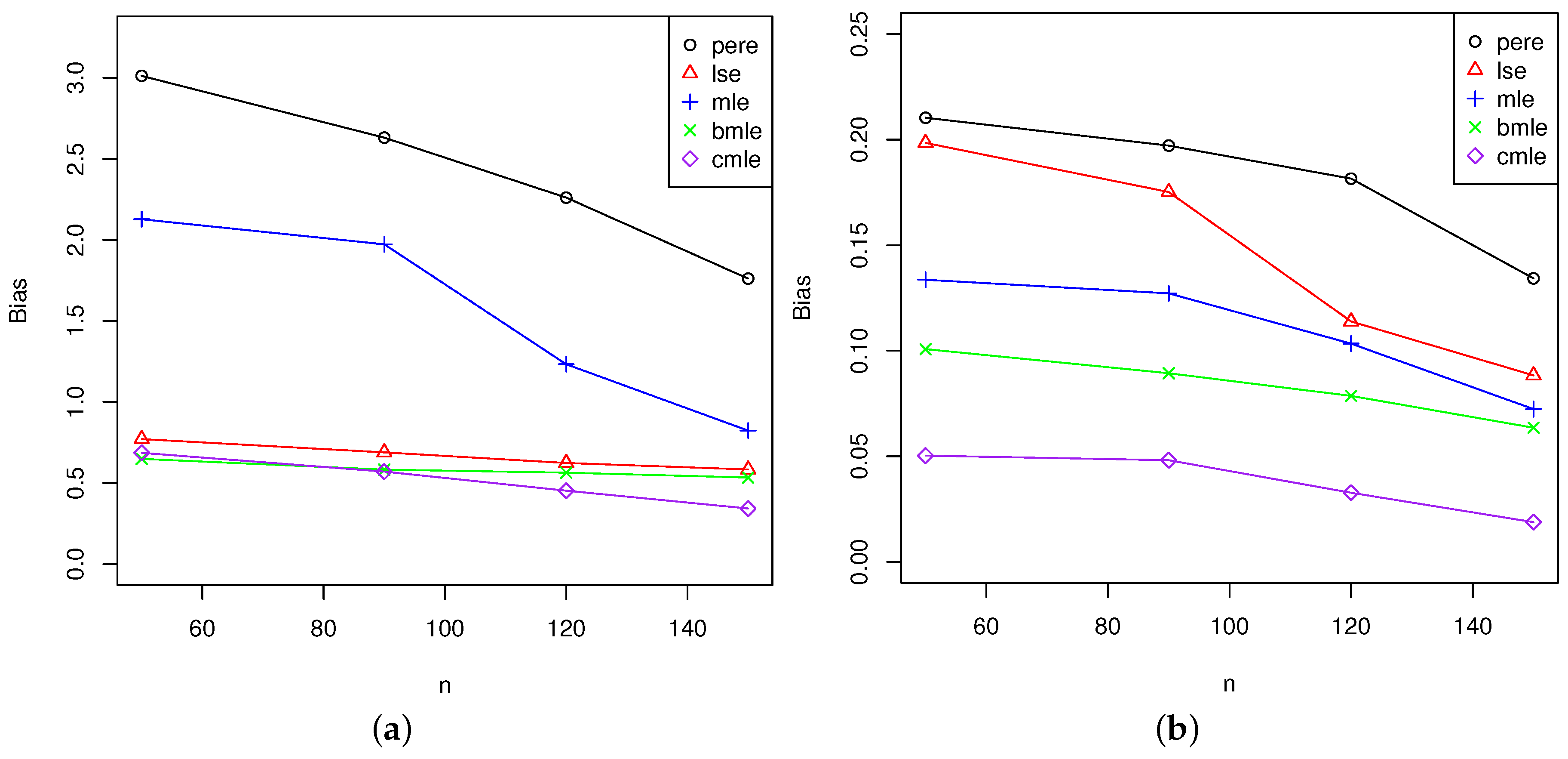
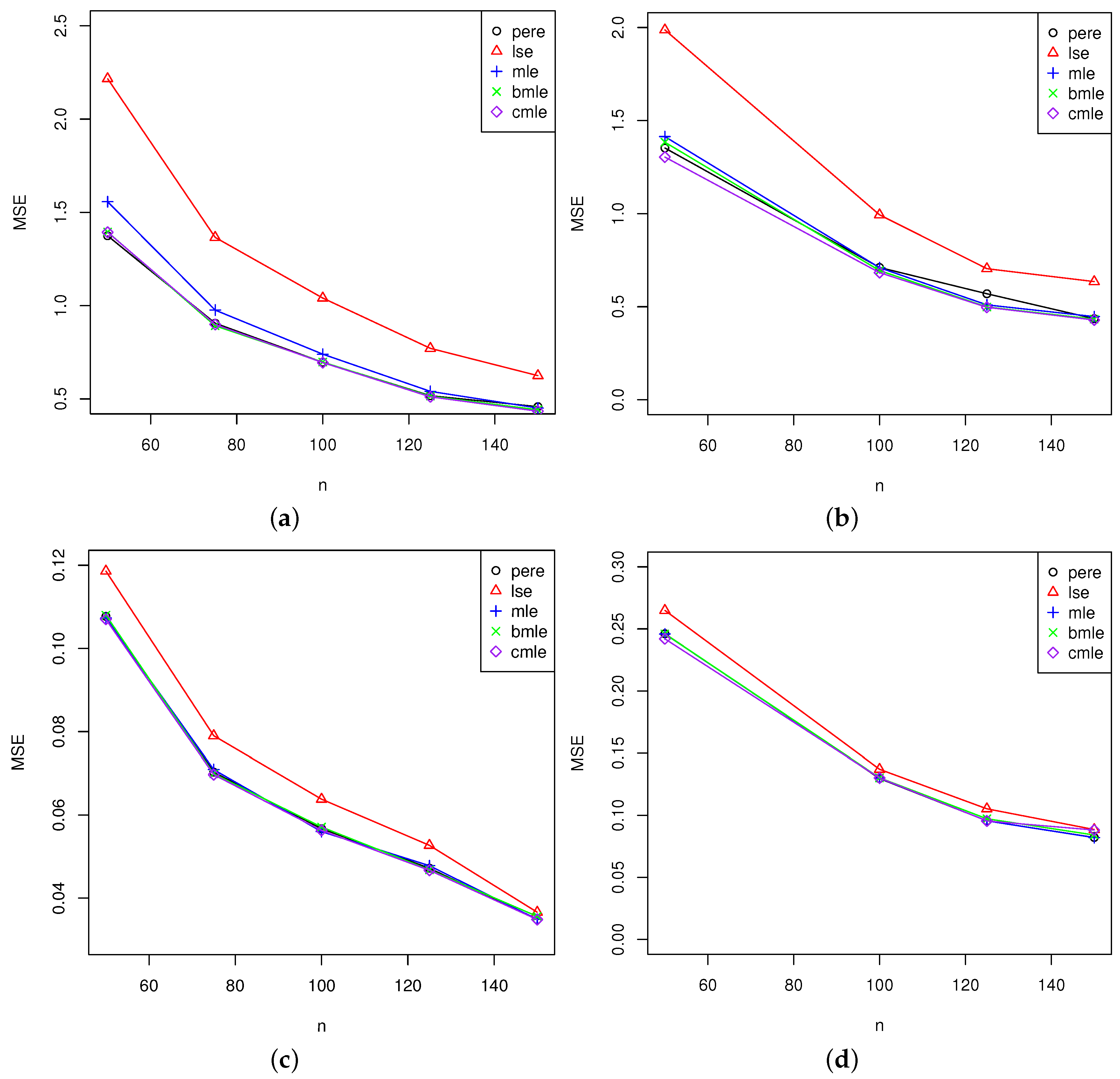
5.2.2. Analysis for All Estimators

The absolute values of the percentage biases of all five estimators are shown in the Figure 1, Figure 2 and Figure 3. Some of the points are clear based on the experimental results. For all methods, as the sample size increases, the biases decrease.
For the most part, the biases of the percentile estimators are larger than those of other estimators, except in specific cases, as shown in Figure 1a and Figure 2a. The bootstrap bias-corrected MLEs and analytic bias-corrected MLEs are generally both superior to MLEs. Furthermore, the analytic bias-corrected MLEs are superior to the other estimators.
The performance of the least squares estimators is uncertain. Sometimes, the least squares estimators perform better than the MLEs, whereas at other times, the latter’s performance stands out. Clearly, the biases of the least squares estimators become extremely similar to those of the bias-corrected MLEs as the sample size increases.
However, the MSEs of the least squares estimators are often larger than those of the other estimators. Meanwhile, the MSEs of the MLEs, analytic bias-corrected MLEs, bootstrap bias-corrected MLEs and percentile estimators are close, as evidenced by the results shown in Figure 4, Figure 5 and Figure 6.
These results indicate that the analytic bias-corrected MLEs can effectively reduce the biases of MLEs. Moreover, to obtain the least biased estimators of the parameters of the Weibull distribution, the analytic bias-corrected MLEs are much more appropriate than the other common estimators mentioned above.

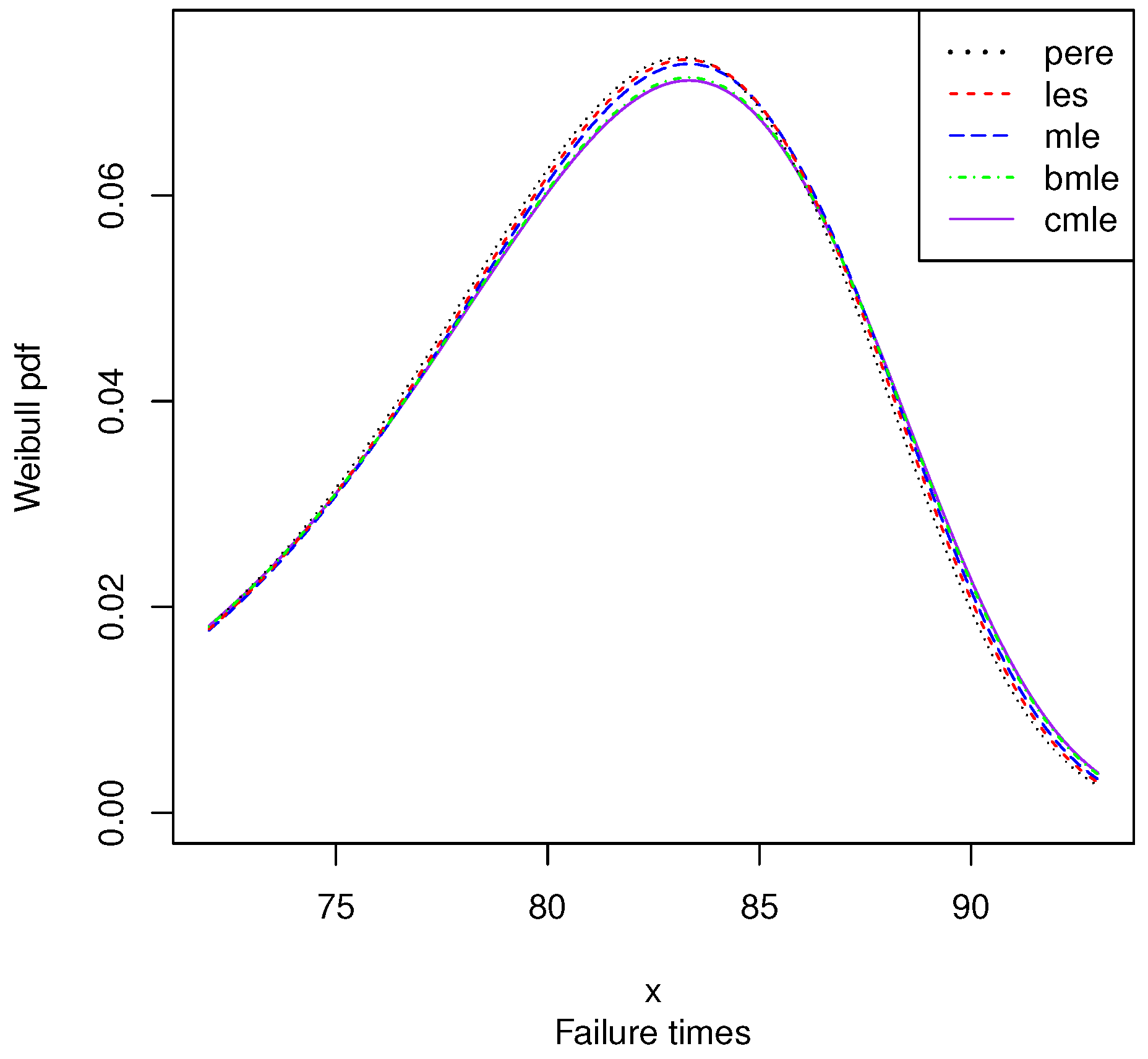
6. Real Illustrative Example

In this section, the practical performance of the Cox–Snell bias correction is explored, and we apply this estimation to real data (i.e., the data provided by Aarest [7]). Aarest tested the times to failure of 50 devices.
We fit the Weibull distribution to these data using MLEs, percentile estimators and least squares estimators. Then, we obtain the bias-corrected parameters by solving the analytic expressions mentioned previously.
Table 3 reports the failure time of 50 devices.
Table 4 reports the maximum likelihood estimates, bootstrap maximum likelihood estimates, analytic bias-corrected maximum likelihood estimates, percentile estimates and least squares estimates after fitting the Weibull distribution to these data.
Based on the MLE of the data shown in Table 3, Figure 7 presents the fitted probability density function curve of Weibull distribution.
For these data, the analytic bias correction decreases the height of the Weibull distribution density, and the shape of the density becomes slightly "fatterr" and "shorter". Thus, the distribution is more uniform.

7. Conclusions

Usually, the two parameters of a Weibull distribution are estimated using maximum likelihood estimation, which is realized under non-linear and first-order conditions. Nevertheless, after comparing all of the methods, it is clear that in terms of the minimization, analytic bias-corrected MLEs exhibited the best performance in almost all cases. Therefore, the analytic bias-corrected MLEs of the two-parameter Weibull distribution are proposed to more effectively reduce the biases of the MLEs.
We conduct a Monte Carlo experiment, which is described in the simulation study section. According to the MSEs and absolute percentage biases of the estimates, we explore the effectiveness of these estimations. Clearly, the biases of the analytic bias-corrected MLEs are smaller than those of the other estimators. Consequently, we can conclude that the analytic bias-corrected MLEs are superior to the others tested here.
All in all, the analytic bias-corrected MLEs discussed in this paper are worth popularizing for utilization on actual data. They should be highly recommended, especially for small sample sizes.

Author Contributions

Man Chen provided main thoughts, organized language, built programming models and did later modifications. Zheng Zhang did investigations, provided practical data, proposed related ideas and polished the language. Cen Cui recorded data and took part in doing programming models and analyzing data.

Conflicts of Interest

The authors declare no conflict of interest.

Appendix A. Specific Calculation

Here are the specific calculation procedures of the bias-corrected MLEs of the parameters of the Weibull distribution.
From the previous part, we can know that the likelihood function of the two-parameter Weibull distribution is:
L = ( 1 λ ) k n k n ( i = 1 n x i ) k 1 e λ k i = 1 n x i k
and the log-likelihood function is:
l = log L = k n log λ + n log k + ( k 1 ) i = 1 n log x i λ k i = 1 n x i k
We obtain these higher-order derivatives:
l λ = k n λ + k λ k 1 i = 1 n x i k
l k = n log λ + n k + i = 1 n log x i λ k i = 1 n x i k log x i + λ k ( log λ ) i = 1 n x i k
2 l λ 2 = k n λ 2 k ( k + 1 ) λ k 2 i = 1 n x i k
2 l k 2 = n k 2 + 2 λ k ( log λ ) i = 1 n x i k log x i λ k i = 1 n x i k ( log x i ) 2 λ k ( log λ ) 2 i = 1 n x i k
2 l λ k = 2 l k λ = n λ + k λ k 1 i = 1 n x i k log x i + ( λ k 1 k λ k 1 log λ ) i = 1 n x i k
3 l λ 3 = 2 k n λ 3 + k ( k + 1 ) ( k + 2 ) λ k 3 i = 1 n x i k
3 l k 3 = 2 n k 3 3 λ k ( log λ ) 2 i = 1 n x i k log x i + 3 λ k ( log λ ) i = 1 n x i k ( log x i ) 2 λ k i = 1 n x i k ( log x i ) 3 + λ k ( log λ ) 3 i = 1 n x i k
3 l λ 2 k = 3 l λ k λ = n λ 2 + ( ( 2 k + 1 ) λ k 2 + k ( k + 1 ) λ k 2 ( log λ ) ) i = 1 n x i k k ( k + 1 ) λ k 2 i = 1 n x i k log λ
3 l k 2 λ = 3 l k λ k = 2 ( λ k 1 k λ k 1 ( log λ ) ) i = 1 n x i k log x i + k λ k 1 i = 1 n x i k ( log x i ) 2 + ( 2 λ k 1 log λ + k λ k 1 ( log λ ) 2 ) i = 1 n x i k
and then, we can obtain the following formulas:
h 11 = E ( 2 l λ 2 )
h 12 = k 21 = E ( 2 l λ k )
h 22 = E ( 2 l k 2 )
The following equations are also easy to get:
E ( i = 1 n x i k ) = n 0 x k ( 1 λ ) k k x k 1 e ( x λ ) k d x = n λ k
E ( i = 1 n x i k log x i ) = n 0 x k l o g x ( 1 λ ) k k x k 1 e ( x λ ) k d x = n λ k ( k log ( λ ) γ + 1 ) k
E ( i = 1 n x i k ( log x i ) 2 ) = n 0 x k ( l o g x ) 2 ( 1 λ ) k k x k 1 e ( x λ ) k d x = n λ k 6 k log ( λ ) ( k log ( λ ) 2 γ + 2 ) + 6 γ ( γ 2 ) + π 2 6 k 2
and the following equation is required for the next calculation part:
E ( i = 1 n x i k ( log x i ) 3 ) = n 0 x k ( log x ) 3 ( 1 λ ) k k x k 1 e ( x λ ) k d x = n λ k ( k log ( λ ) ( 2 k log ( λ ) ( k log ( λ ) 3 γ + 3 ) + 6 γ ( γ 2 ) + π 2 ) 4 ζ ( 3 ) γ ( 2 γ ( γ 3 ) + π 2 ) + π 2 ) 2 k 3
Where γ is a constant called eulergamma and its value is about 0.57721; and ζ ( 3 ) is another constant, and its value is about 1.20206; then, these results can be obtained:
h 11 = k 2 n λ 2 , h 12 = h 21 = ( 1 γ ) n λ , h 22 = 6 γ 2 12 γ + π 2 + 6 n 6 k 2
Then, based on Equation (16), a series of results is obtained:
h 11 1 = h 11 λ = 2 h 2 n λ 3
h 12 1 = h 21 1 = h 12 λ = ( γ 1 ) n λ 2
h 22 1 = h 22 λ = 0
h 11 2 = h 11 k = 2 k n λ 2
h 12 2 = h 21 2 = h 12 h = 0    
       h 22 2 = h 22 k = ( 6 12 γ + 6 γ 2 + π 2 ) n 3 k 3
h 111 = k 2 ( k + 3 ) n λ 3
h 122 = h 212 = h 221 = 12 24 γ + 6 γ 2 + π 2 n 6 k λ
      h 222 = n 4 ζ ( 3 ) + 2 γ 3 6 γ 2 + γ π 2 π 2 + 4 2 k 3
then:
a 11 ( 1 ) = h 11 1 1 2 h 111 = ( k 1 ) k 2 n 2 λ 3   
a 12 ( 1 ) = h 12 1 1 2 h 121 = ( γ k + 3 k + γ 1 ) n 2 λ 2
a 21 ( 1 ) = h 21 1 1 2 h 211 = ( γ k + 3 k + γ 1 ) n 2 λ 2
a 22 ( 1 ) = h 22 1 1 2 h 221 = ( 12 24 γ + 6 γ 2 + π 2 ) n 12 k λ
a 11 ( 2 ) = h 11 2 1 2 h 112 = ( γ k + k + γ 1 ) n 2 λ 2   
a 12 ( 2 ) = h 12 2 1 2 h 122 = ( 12 24 γ + 6 γ 2 + π 2 ) n 12 k λ
a 21 ( 2 ) = h 21 2 1 2 h 212 = ( 12 24 γ + 6 γ 2 + π 2 ) n 12 k λ
a 22 ( 2 ) = h 22 2 1 2 h 222 = n ( 12 ζ ( 3 ) + 3 γ ( 8 + π 2 ) + 6 γ 3 30 γ 2 5 π 2 ) 6 k 3
From the formula H i j = { h i j } , we can know that the information matrix is:
H = k 2 n λ 2 ( 1 γ ) n λ ( 1 γ ) n λ 6 γ 2 12 γ + π 2 + 6 n 6 k 2
and:
A = [ A ( 1 ) A ( 2 ) ]
A = a 11 ( 1 ) a 12 ( 1 ) a 11 ( 2 ) a 12 ( 2 ) a 21 ( 1 ) a 22 ( 1 ) a 21 ( 2 ) a 22 ( 2 )
Using the bias-corrected expressions in the matrix form, we can obtain:
B i a s λ ^ k ^ = σ ^ H ^ 1 A ^ v e c ( H ^ 1 )
The bias-corrected estimates are:
λ ˜ k ˜ = λ ^ k ^ B i a s λ ^ k ^
where H ^ = H | λ = λ ^ , k = k ^ , A ^ = A | λ = λ ^ , k = k ^

References

  1. Rosin, P.O.; Rammler, E.J. The Laws Governing the Fineness of Powdered Coal. J. Inst. Fuel 1933, 7, 29–36. [Google Scholar]
  2. Ling, X.; Giles, D.E. Bias Reduction for the Maximum Likelihood Estimator of the Parameters of the Generalized Rayleigh Family of Distributions. Commun. Stat. Theory Methods 2009, 43, 1778–1792. [Google Scholar] [CrossRef]
  3. Fréchet, M. Sur la loi de Probabilité de Lécart Maximum. Ann. Soc. Pol. Math. 1927, 6, 93–116. [Google Scholar]
  4. Kaltschmidt, E.; Dzionara, M.; Donner, D.; Wittmann, H.G. Application of the Weibull Distribution on the Evaluation of the Aircraft System Operational Reliability. Mol. Gen. Genet. MGG 1967, 100, 364–373. [Google Scholar] [CrossRef] [PubMed]
  5. Mikolaj, P.G. Environmental applications of the weibull distribution function: Oil pollution. Science 1972, 176, 1019–1021. [Google Scholar] [CrossRef] [PubMed]
  6. Singh, V.P. On application of the Weibull distribution in hydrology. Water Resour. Manag. 1987, 1, 33–43. [Google Scholar] [CrossRef]
  7. Aarset, M.V. How to identify a bathtub hazard rate. IEEE Trans. Reliab. 1987, R-36, 106–108. [Google Scholar] [CrossRef]
  8. Lai, C.D.; Xie, M.; Murthy, D.N.P. A Modified Weibull Distribution. IEEE Trans. Reliab. 2003, 52, 33–37. [Google Scholar] [CrossRef]
  9. Hirose, H. Maximum likelihood parameter estimation in the extended Weibull distribution and its applications to breakdown voltage estimation. IEEE Trans. Dielectr. Electr. Insul. 2002, 9, 524–536. [Google Scholar] [CrossRef]
  10. Fabiani, D.; Simoni, L. Discussion on application of the Weibull distribution to electrical breakdown of insulating materials. IEEE Trans. Dielectr. Electr. Insul. 2005, 12, 11–16. [Google Scholar] [CrossRef]
  11. Ghitany, M.E.; Al-Jarallah, A.H.R.A. Marshall-Olkin extended Weibull distribution and its application to censored data. J. Appl. Stat. 2005, 32, 1025–1034. [Google Scholar] [CrossRef]
  12. Akdaǧ, S.A.; Dinler, A. A new method to estimate Weibull parameters for wind energy applications. Energy Convers. Manag. 2009, 50, 1761–1766. [Google Scholar] [CrossRef]
  13. Cox, D.R.; Snell, E.J. A general definition of residuals. J. R. Stat. Soc. 1968, 30, 248–275. [Google Scholar]
  14. Cordeiro, G.M.; Klein, R. Bias correction in ARMA models. Stat. Probab. Lett. 1994, 19, 169–176. [Google Scholar] [CrossRef]
  15. Giles, D.E. Bias-corrected maximum likelihood estimation of the parameters of the generalized Pareto distribution. Commun. Stat. Theory Methods 2012, 45, 2465–2483. [Google Scholar] [CrossRef]
  16. Wang, M.; Wang, W. Bias-corrected Maximum Likelihood Estimation of the Parameters of the Weighted Lindley Distribution. Commun. Stat. Simul. Comput. 2017, 46, 530–545. [Google Scholar] [CrossRef]
  17. Mackinnon, J.G.; Smith, A.A. Approximate bias corrections in econometrics. J. Econom. 1998, 85, 205–230. [Google Scholar] [CrossRef]
  18. Ferrari, S.; Cribari-Neto, F. On bootstrap and analytical bias corrections. Econ. Lett. 1998, 58, 7–15. [Google Scholar] [CrossRef]
  19. Ho, L.L.; da Silva, A.F. Bias Correction for Mean Time to Failure and p-Quantiles in a Weibull Distribution by Bootstrap Procedure. Commun. Stat. Simul. Comput. 2005, 34, 617–629. [Google Scholar] [CrossRef]
  20. Focarelli, D. Bootstrap bias-corrected estimators to investigate the long-run properties of money demand in the euro area. Econ. Model. 2002, 22, 305–325. [Google Scholar] [CrossRef]
  21. Kao, J.H.K. Computer Methods for Estimating Weibull Parameters in Reliability Studies. IRE Trans. Reliab. Qual. Control 1958, 13, 15–22. [Google Scholar] [CrossRef]
  22. Kao, J.H.K. A Graphical Estimation of Mixed Weibull Parameters in Life-Testing of Electron Tubes. Technometrics 1959, 1, 389–407. [Google Scholar] [CrossRef]
  23. Mann, N.R.; Schafer, R.E.; Singpurwalla, N.D. Methods for statistical analysis of reliability and life data. J. R. Stat. Soc. 1974, 139, 1974. [Google Scholar]
  24. Gupta, R.D.; Kundu, D. Generalized exponential distribution: Different method of estimations. J. Stat. Comput. Simul. 2001, 69, 315–337. [Google Scholar] [CrossRef]
  25. Swain, J.; Venkatraman, S.; Wilson, J.R. Least-squares estimation of distribution function in Johnson’s translation system. J. Stat. Comput. Simul. 1988, 29, 271–297. [Google Scholar] [CrossRef]
  26. Johnson, N.L.; Kotz, S.; Balakrishnan, N. Continuous Univariate Distributions; John Wiley & Sons: New York, NY, USA, 1994. [Google Scholar]
  27. Murdoch, D. R-3.2.2 for Windows. Available online: https://cran.r-project.org/bin/windows/base/old/3.2.2/ (accessed on 27 August 2015).
Figure 1. % Bias of the parameters. (a) % Bias of k ( k = 4 . 5 , λ = 2 . 5 ); (b) % bias of k ( k = 3 , λ = 5 ); (c) % bias of λ ( k = 4 . 5 , λ = 2 . 5 ); (d) % bias of λ ( k = 3 , λ = 5 ). In these figures, pere, lse, mle, bmle and mle denote the related curves of percentile estimators, least squares estimators, MLEs, bootstrap corrected MLEs and analytic bias-corrected estimators.
Mca 22 00019 g001
Figure 2. % Bias of the parameters. (a) % bias of k ( k = 5 . 8 , λ = 4 ); (b) % bias of λ ( k = 5 . 8 , λ = 4 ); (c) % bias of k ( k = 3 , λ = 2 . 6 ); (d) % bias of λ ( k = 3 , λ = 2 . 6 ).
Mca 22 00019 g002
Figure 3. % Bias of the parameters. (a) % bias of k ( k = 16 , λ = 83 . 8 ); (b) % bias of λ ( k = 16 , λ = 83 . 8 ).
Mca 22 00019 g003
Figure 4. % MSEs of the parameters. (a) % MSE of k ( k = 4 . 5 , λ = 2 . 5 ); (b) % MSE of k ( k = 3 , λ = 5 ); (c) % MSE of λ ( k = 4 . 5 , λ = 2 . 5 ); (d) % MSE of λ ( k = 3 , λ = 5 ).
Mca 22 00019 g004
Figure 5. % MSEs of the parameters. (a) % MSE of k ( k = 5 . 8 , λ = 4 ); (b) % MSE of λ ( k = 5 . 8 , λ = 4 ); (c) % MSE of k ( k = 3 , λ = 2 . 6 ); (d) % MSE of λ ( k = 3 , λ = 5 ).
Mca 22 00019 g005aMca 22 00019 g005b
Figure 6. % MSEs of the parameters. (a) % MSE of k ( k = 16 , λ = 83 . 8 ); (b) % MSE of k ( k = 16 , λ = 83 . 8 ).
Mca 22 00019 g006
Figure 7. Fitted Weibull’s probability density function (failure time data).
Mca 22 00019 g007
Table 1. Percentage bias and mean squared errors (MSEs) for the exponential distribution.
n k ^ k Per k ˇ k Lse k ˜
k = 1 , λ = 4 . 2 10 3 . 38797 ( 1 . 72263 ) 4 . 24687 ( 1 . 63461 ) 1 . 62722 ( 1 . 68783 ) 2 . 03847 ( 2 . 23278 ) 1 . 54944 ( 2 . 178493 )
20 3 . 29136 ( 1 . 65143 ) 4 . 13135 ( 1 . 57272 ) 1 . 58273 ( 1 . 52827 ) 1 . 74331 ( 2 . 177534 ) 1 . 48638 ( 1 . 40788 )
50 2 . 79397 ( 1 . 14223 ) 3 . 64087 ( 1 . 09408 ) 1 . 09148 ( 1 . 04746 ) 1 . 21462 ( 1 . 68899 ) 0 . 97849 ( 0 . 98887 )
90 2 . 25832 ( 0 . 43723 ) 2 . 73324 ( 0 . 49677 ) 1 . 03022 ( 0 . 41751 ) 1 . 09139 ( 0 . 95252 ) 0 . 96362 ( 0 . 40429 )
k = 1 , λ = 6 10 3 . 62346 ( 2 . 43225 ) 4 . 52579 ( 2 . 32371 ) 1 . 93752 ( 2 . 37691 ) 2 . 12836 ( 2 . 84987 ) 1 . 83741 ( 2 . 23637 )
20 3 . 48225 ( 2 . 34162 ) 4 . 44257 ( 2 . 26101 ) 1 . 84247 ( 2 . 23775 ) 1 . 93243 ( 2 . 76782 ) 1 . 73236 ( 2 . 19606 )
50 2 . 48276 ( 1 . 83342 ) 3 . 33175 ( 1 . 71529 ) 0 . 99447 ( 1 . 75702 ) 1 . 01764 ( 2 . 37791 ) 0 . 96848 ( 1 . 67906 )
90 2 . 24721 ( 0 . 88253 ) 2 . 92384 ( 0 . 89496 ) 0 . 83833 ( 0 . 89241 ) 0 . 99847 ( 1 . 04731 ) 0 . 81751 ( 0 . 81043 )
n λ ^ λ Per λ ˇ λ Lse λ ˜
k = 1 , λ = 4 . 2 10 0 . 32264 ( 0 . 24035 ) 0 . 28236 ( 0 . 59336 ) 0 . 623731 ( 0 . 24071 ) 0 . 18357 ( 0 . 30108 ) 0 . 17435 ( 0 . 23218 )
20 0 . 31451 ( 0 . 22341 ) 0 . 27293 ( 0 . 23809 ) 0 . 24386 ( 0 . 23353 ) 0 . 17673 ( 0 . 29049 ) 0 . 16212 ( 0 . 22234 )
50 0 . 27232 ( 0 . 18334 ) 0 . 22251 ( 0 . 18124 ) 0 . 19474 ( 0 . 18364 ) 0 . 12734 ( 0 . 24157 ) 0 . 11615 ( 0 . 17787 )
90 0 . 22582 ( 0 . 13205 ) 0 . 21523 ( 0 . 13221 ) 0 . 16342 ( 0 . 13201 ) 0 . 09862 ( 0 . 15193 ) 0 . 06783 ( 0 . 12996 )
k = 1 , λ = 6 10 0 . 23464 ( 0 . 22826 ) 0 . 36204 ( 0 . 23118 ) 0 . 19424 ( 0 . 22719 ) 0 . 35411 ( 0 . 23386 ) 0 . 13571 ( 0 . 22105 )
20 0 . 21527 ( 0 . 21376 ) 0 . 34482 ( 0 . 21096 ) 0 . 18895 ( 0 . 21855 ) 0 . 33206 ( 0 . 22596 ) 0 . 12556 ( 0 . 21224 )
50 0 . 20738 ( 0 . 19892 ) 0 . 28401 ( 0 . 20515 ) 0 . 17804 ( 0 . 19497 ) 0 . 26589 ( 0 . 20787 ) 0 . 12404 ( 0 . 19272 )
90 0 . 19278 ( 0 . 09642 ) 0 . 26276 ( 0 . 09994 ) 0 . 15497 ( 0 . 09036 ) 0 . 24259 ( 0 . 10425 ) 0 . 11285 ( 0 . 08902 )
In these tables λ ^ , λ P e r , λ ˇ , λ L s e , λ ˜ denote MLEs, percentile, bootstrap, least squares and analytic bias corrected estimators of λ.
Table 2. Percentage bias and MSEs for the Weibull distribution.
n k ^ k Per k ˇ k Lse k ˜
k = 3 , λ = 5 10 2 . 87878 ( 2 . 02135 ) 3 . 76377 ( 1 . 94205 ) 1 . 17121 ( 1 . 97737 ) 1 . 58273 ( 2 . 52286 ) 1 . 09343 ( 0 . 48693 )
20 2 . 71862 ( 1 . 91433 ) 3 . 61252 ( 1 . 82626 ) 1 . 02736 ( 1 . 88171 ) 1 . 23402 ( 2 . 47634 ) 0 . 96782 ( 1 . 77987 )
50 2 . 23878 ( 1 . 42331 ) 3 . 10377 ( 1 . 34989 ) 0 . 51983 ( 1 . 37363 ) 0 . 74025 ( 1 . 98798 ) 0 . 48693 ( 1 . 28777 )
90 1 . 78422 ( 0 . 77231 ) 2 . 23241 ( 0 . 76976 ) 0 . 50221 ( 0 . 77014 ) 0 . 51992 ( 1 . 22424 ) 0 . 46362 ( 0 . 74991 )
120 1 . 33244 ( 0 . 68769 ) 1 . 76234 ( 0 . 55237 ) 0 . 49025 ( 0 . 52129 ) 0 . 52106 ( 0 . 76348 ) 0 . 38221 ( 0 . 50104 )
k = 4 . 5 , λ = 2 . 5 10 4 . 46931 ( 2 . 83411 ) 3 . 27236 ( 2 . 49953 ) 2 . 72193 ( 2 . 38278 ) 1 . 98214 ( 3 . 40137 ) 0 . 56310 ( 2 . 22179 )
20 4 . 21625 ( 2 . 61951 ) 2 . 92736 ( 2 . 27636 ) 2 . 51293 ( 2 . 15254 ) 1 . 68174 ( 3 . 19227 ) 0 . 54212 ( 2 . 00913 )
50 3 . 34629 ( 1 . 58012 ) 2 . 16325 ( 1 . 37882 ) 1 . 13245 ( 1 . 37627 ) 0 . 80234 ( 2 . 2101 ) 0 . 49672 ( 1 . 37421 )
90 2 . 22365 ( 0 . 78163 ) 1 . 49237 ( 0 . 70841 ) 0 . 82329 ( 0 . 70527 ) 0 . 62342 ( 1 . 22716 ) 0 . 48297 ( 0 . 70044 )
120 1 . 83167 ( 0 . 57310 ) 1 . 26119 ( 0 . 56236 ) 0 . 58293 ( 0 . 56093 ) 0 . 45231 ( 0 . 76328 ) 0 . 41032 ( 0 . 55047 )
k = 16 , λ = 83 . 8 10 3 . 36463 ( 2 . 51351 ) 4 . 25296 ( 2 . 43116 ) 1 . 67224 ( 2 . 46618 ) 1 . 88162 ( 2 . 99377 ) 1 . 57213 ( 2 . 36262 )
20 3 . 11751 ( 2 . 41325 ) 4 . 12374 ( 2 . 31519 ) 1 . 52373 ( 2 . 37256 ) 1 . 61233 ( 2 . 87527 ) 1 . 42262 ( 2 . 26869 )
50 2 . 12766 ( 1 . 93223 ) 3 . 01256 ( 1 . 85091 ) 0 . 64873 ( 1 . 87429 ) 0 . 77045 ( 2 . 47618 ) 0 . 68583 ( 1 . 79669 )
90 1 . 97311 ( 0 . 92734 ) 2 . 63147 ( 0 . 94868 ) 0 . 58232 ( 0 . 92813 ) 0 . 68873 ( 1 . 17312 ) 0 . 57014 ( 0 . 90033 )
120 1 . 23241 ( 0 . 69887 ) 1 . 26123 ( 0 . 58363 ) 0 . 56344 ( 0 . 57314 ) 0 . 62323 ( 0 . 73139 ) 0 . 45236 ( 0 . 50315 )
n λ ^ λ Per λ ˇ λ Lse λ ˜
k = 3 , λ = 5 10 0 . 28614 ( 0 . 26124 ) 0 . 241226 ( 0 . 61216 ) 0 . 211832 ( 0 . 26081 ) 0 . 146316 ( 0 . 32004 ) 0 . 135225 ( 0 . 25109 )
20 0 . 27369 ( 0 . 25233 ) 0 . 23311 ( 0 . 25917 ) 0 . 20496 ( 0 . 25164 ) 0 . 13753 ( 0 . 31193 ) 0 . 12613 ( 0 . 24765 )
50 0 . 23112 ( 0 . 20114 ) 0 . 18432 ( 0 . 20213 ) 0 . 15589 ( 0 . 20175 ) 0 . 08864 ( 0 . 26232 ) 0 . 07725 ( 0 . 19897 )
90 0 . 17768 ( 0 . 15408 ) 0 . 175003 ( 0 . 15431 ) 0 . 12795 ( 0 . 15201 ) 0 . 07716 ( 0 . 17203 ) 0 . 02694 ( 0 . 15097 )
120 0 . 11291 ( 0 . 11124 ) 0 . 13766 ( 0 . 11214 ) 0 . 67633 ( 0 . 11072 ) 0 . 02675 ( 0 . 11482 ) 0 . 01418 ( 0 . 10621 )
k = 4 . 5 , λ = 2 . 5 10 0 . 19743 ( 0 . 13385 ) 0 . 310213 ( 0 . 14019 ) 0 . 15342 ( 0 . 13291 0 . 321029 ( 0 . 14933 ) 0 . 08721 ( 0 . 13004 )
20 0 . 17243 ( 0 . 12724 ) 0 . 29126 ( 0 . 12948 ) 0 . 14191 ( 0 . 12574 ) 0 . 30927 ( 0 . 13852 ) 0 . 08512 ( 0 . 12121 )
50 0 . 15672 ( 0 . 10983 ) 0 . 22125 ( 0 . 11032 0 . 11814 ( 0 . 10875 ) 0 . 20923 ( 0 . 11763 ) 0 . 07431 ( 0 . 10814 )
90 0 . 12609 ( 0 . 06171 ) 0 . 20823 ( 0 . 06182 ) 0 . 08726 ( 0 . 06121 ) 0 . 17301 ( 0 . 07124 ) 0 . 04814 ( 0 . 06908 )
120 0 . 10203 ( 0 . 05097 ) 0 . 18037 ( 0 . 05102 ) 0 . 73716 ( 0 . 05092 ) 0 . 09272 ( 0 . 05782 ) 0 . 03223 ( 0 . 05073 )
k = 16 , λ = 83 . 8 10 0 . 16632 ( 0 . 25277 ) 0 . 29013 ( 0 . 26126 ) 0 . 12231 ( 0 . 25163 ) 0 . 28137 ( 0 . 26897 ) 0 . 06746 ( 0 . 25005 )
20 0 . 14243 ( 0 . 24724 ) 0 . 27839 ( 0 . 24997 ) 0 . 11978 ( 0 . 24578 ) 0 . 26015 ( 0 . 25942 ) 0 . 05542 ( 0 . 24213 )
50 0 . 13362 ( 0 . 22975 ) 0 . 21037 ( 0 . 23141 ) 0 . 10077 ( 0 . 22934 ) 0 . 19845 ( 0 . 23861 ) 0 . 05031 ( 0 . 22711 )
90 0 . 12717 ( 0 . 12457 ) 0 . 19715 ( 0 . 12986 ) 0 . 08934 ( 0 . 12397 ) 0 . 17518 ( 0 . 13232 ) 0 . 04814 ( 0 . 12182 )
120 0 . 10336 ( 0 . 08319 ) 0 . 18513 ( 0 . 09043 ) 0 . 07861 ( 0 . 08126 ) 0 . 11388 ( 0 . 12123 ) 0 . 03272 ( 0 . 07964 )
n k ^ k Per k ˇ k Lse k ˜
k = 5 . 8 , λ = 4 10 4 . 66337 ( 2 . 99373 ) 3 . 32984 ( 2 . 79688 ) 2 . 60702 ( 3 . 72264 ) 1 . 59874 ( 3 . 42664 ) 0 . 88434 ( 2 . 81625 )
20 4 . 37652 ( 2 . 86477 ) 3 . 11147 ( 2 . 43241 ) 2 . 47002 ( 3 . 28695 ) 1 . 45287 ( 3 . 05669 ) 0 . 67798 ( 2 . 53676 )
50 3 . 29761 ( 1 . 71237 ) 2 . 42056 ( 1 . 51879 ) 1 . 68072 ( 2 . 37586 ) 1 . 06739 ( 2 . 13422 ) 0 . 58241 ( 1 . 51003 )
90 2 . 02482 ( 0 . 66934 ) 1 . 69243 ( 0 . 65832 ) 0 . 75016 ( 0 . 69897 ) 0 . 51206 ( 1 . 21028 ) 0 . 49431 ( 0 . 50207 )
120 1 . 55471 ( 0 . 52901 ) 1 . 24899 ( 0 . 53106 ) 0 . 71538 ( 0 . 52411 ) 0 . 41097 ( 0 . 61093 ) 0 . 39275 ( 0 . 511364 )
k = 3 , λ = 2 . 6 10 0 . 28441 ( 2 . 03217 ) 0 . 19927 ( 2 . 00121 ) 0 . 19221 ( 1 . 96287 ) 0 . 14282 ( 2 . 56542 ) 0 . 13155 ( 0 . 95892 )
20 0 . 27233 ( 1 . 92128 ) 0 . 18876 ( 1 . 90851 ) 0 . 18024 ( 1 . 89326 ) 0 . 12393 ( 2 . 47998 ) 0 . 11042 ( 1 . 88297 )
50 0 . 22341 ( 1 . 40236 ) 0 . 17543 ( 1 . 38972 ) 1 . 15976 ( 1 . 37653 ) 0 . 09472 ( 1 . 87524 ) 0 . 07424 ( 1 . 36891 )
90 0 . 16493 ( 0 . 85237 ) 0 . 16998 ( 0 . 75364 ) 0 . 11978 ( 0 . 74984 ) 0 . 06921 ( 1 . 10475 ) 0 . 02602 ( 0 . 74004 )
120 0 . 11419 ( 0 . 51264 ) 0 . 14235 ( 0 . 50928 ) 0 . 07321 ( 0 . 50886 ) 0 . 02634 ( 0 . 75213 ) 0 . 02123 ( 0 . 50832 )
n λ ^ λ Per λ ˇ λ Lse λ ˜
k = 5 . 8 , λ = 4 10 0 . 23323 ( 0 . 99762 ) 0 . 25986 ( 1 . 03875 ) 0 . 10375 ( 1 . 08632 ) 0 . 25671 ( 1 . 12056 ) 0 . 07796 ( 0 . 97432 )
20 0 . 22505 ( 0 . 96251 ) 0 . 24158 ( 0 . 98347 ) 0 . 09865 ( 0 . 99879 ) 0 . 24763 ( 1 . 03522 ) 0 . 06987 ( 0 . 94318 )
50 0 . 15613 ( 0 . 65838 ) 0 . 20069 ( 0 . 66927 ) 0 . 08976 ( 0 . 67832 ) 0 . 20973 ( 0 . 74224 ) 0 . 05759 ( 0 . 65021 )
90 0 . 11203 ( 0 . 34578 ) 0 . 15563 ( 0 . 34865 ) 0 . 07783 ( 0 . 34196 ) 0 . 15107 ( 0 . 38976 ) 0 . 04326 ( 0 . 33275 )
120 0 . 09463 ( 0 . 02524 ) 0 . 13374 ( 0 . 02637 ) 0 . 06372 ( 0 . 02496 ) 0 . 13214 ( 0 . 03109 ) 0 . 02543 ( 0 . 02387 )
k = 3 , λ = 2 . 6 10 0 . 59711 ( 0 . 39213 ) 0 . 48897 ( 0 . 40027 ) 0 . 38799 ( 0 . 37994 ) 0 . 466206 ( 0 . 42374 ) 0 . 27911 ( 0 . 38133 )
20 0 . 56192 ( 0 . 28192 ) 0 . 45256 ( 0 . 38627 ) 0 . 34521 ( 0 . 35879 ) 0 . 44575 ( 0 . 39266 ) 0 . 21364 ( 0 . 35025 )
50 0 . 32624 ( 0 . 25173 ) 0 . 39201 ( 0 . 25086 ) 0 . 23336 ( 0 . 24965 ) 0 . 35214 ( 0 . 27894 ) 0 . 13342 ( 0 . 24837 )
90 0 . 11398 ( 0 . 13021 ) 0 . 32325 ( 0 . 13264 ) 0 . 10924 ( 0 . 12987 ) 0 . 22343 ( 0 . 15036 ) 0 . 05121 ( 0 . 12866 )
120 0 . 79112 ( 0 . 0987 ) 0 . 14923 ( 0 . 07023 ) 0 . 08011 ( 0 . 06973 ) 0 . 09234 ( 0 . 08997 ) 0 . 01206 ( 0 . 06835 )
Table 3. Calculated failure time of 50 devices.
No.12345678910111213
0.1007.0036.0067.0084.000.20011.0040.0067.0084.001.0012.0045.00
No.14151617181920212223242526
67.0084.001.0018.0046.0067.0085.001.0018.0047.0072.0085.001.00
No.27282930313233343536373839
18.0050.0075.0085.001.0018.0055.0079.0085.002.0018.0060.0082.00
No.4041424344454647484950
85.003.0021.0063.0082.0086.006.0032.0063.0083.0086.00
Table 4. Five estimates of Parameters.
k ^ k Per k ˇ k Lse k ˜
16.5217516.6314516.2212516.6023516.15814
λ ^ λ Per λ ˇ λ Lse λ k
83.6460183.4811483.65511483.5811483.669204

