Spatiotemporal Dynamics of a Delayed and Diffusive Viral Infection Model with Logistic Growth

Abstract

Viruses have important influences on human health: they not only cause some common diseases, but also cause serious illnesses. Moreover, the conventional medicines usually fail to prevent or treat them, and viral infections are hard to treat because viruses live inside the body’s cells. However, some mathematical models can help to understand the viral transmission mechanism and control viral diseases. In this paper, a delayed viral infection model with spatial diffusion and logistic growth is presented. The asymptotic stability of nonnegative uniform steady states is investigated by utilizing the linearized method and constructing the proper Lyapunov functional, respectively. The existence of Hopf bifurcation from the positive equilibrium point is established by analyzing the corresponding characteristic equation and the direction of bifurcation, and the properties of bifurcating periodic solutions are derived by the aid of the normal form theory for partial functional differential equations. Then, the cross-diffusion system is introduced. Furthermore, some numerical simulations are carried, out and discussions are given.

1. Introduction

Viruses are found wherever there is life and have probably existed since living cells first evolved [1]. A virus is a small infectious agent that replicates only inside the living cells of other organisms. Viruses can infect all types of life forms, from animals and plants to microorganisms, including bacteria and archaea [2].

A viral infection occurs when an organism’s body is invaded by pathogenic viruses, and infectious virus particles (virions) attach to and enter susceptible cells [3]. Viruses have extensive biochemical effects on the host cells. Most virus infections eventually result in the death of the host cells, such as human immunodeficiency virus, human papillomavirus, and so on. Some viruses can also cause lifelong or chronic infections, which is common in hepatitis B virus and hepatitis C virus infections. All in all, once someone is infected by such viruses, physical health might suffer.

At present, the research on the dynamics of viral infection models has been one of the most challenging directions in the field of mathematical epidemiology; it is very important and very significative. For a quantitative analysis of these viral infections, Nowak and co-workers [4,5] designed the basic mathematical model based on the ordinary differential equations was designed as follows:

$${\displaystyle \left\{\begin{array}{c}\frac{du}{dt}=\lambda -du-\beta uv,\hfill \\ \frac{dw}{dt}=\beta uv-aw,\hfill \\ \frac{dv}{dt}=kw-cv,\hfill \end{array}\right.}$$

(1)

where the dependent variables u, w and v represent the population of uninfected target cells, the population of infected cells and the population of free virus particles. It is supposed that the target cells are supplied at a constant rate λ, and they are removed either through cell death with death rate d or by becoming infected by virions. The parameter β is the rate of infection of target cells per virion; k represents the number of virions produced per unit time, per infected cell; a is the death rate of the infected cells; and c is the clearance rate of virions.

A great deal of generalized forms have been developed by various scholars in accordance with the basic model (1). For instance, Wang et al. [6] considered an improved hepatitis B virus model with standard incidence function and a cytokine-mediated cure, and they obtained the global stability of infection-free and infection equilibria. Tian and Xu [7] studied the asymptotic behaviors of a viral infection model with time delay and standard incidence function. Wang and Tian [8] formulated a delayed hepatitis B virus infection model incorporating three components: susceptible cells, infected cells and virus-specific cytotoxic T lymphocyte cells (CTLs). Gourley et al. [9] and Eikenberry et al. [10] investigated the effect of the latent infected period on the viral infection models. Besides, Eric et al. [11] gave a delayed viral infection model with mitosis transmission and established the stability of the system and the occurrence of Hopf bifurcation. Qesmi et al. [12] proposed a liver-virus-blood model to describe infection in both liver and blood, and they have discussed the basic properties of the system and the existence of backward bifurcation. Ahmed and El-Saka [13] also presented and discussed a fractional order hepatitis C virus model.

Although System (1) and its generalized forms have described the basic viral infection relations among the cells and viruses, the quasispecies here is not usually well mixed, and the mobility of cells and viruses cannot be ignored. Indeed, biological motion plays a crucial role in many biological phenomena [14]. The famous Turing instability, which was first proposed in [15], is the archetypical behavior driven by spatial diffusion. Therefore, Wang and co-workers [16,17] introduced the random mobility of viruses into (1) and considered the following non-dimensional diffusive model:

$${\displaystyle \left\{\begin{array}{c}\frac{\mathsf{\partial }u(x,t)}{\mathsf{\partial }t}=1-u(x,t)-u(x,t)v(x,t),\hfill \\ \frac{\mathsf{\partial }w(x,t)}{\mathsf{\partial }t}=u(x,t-\tau )v(x,t-\tau )-{\rho }_{1}w(x,t),\hfill \\ \frac{\mathsf{\partial }v(x,t)}{\mathsf{\partial }t}=D\Delta v(x,t)+{\rho }_{2}w(x,t)-{\rho }_{3}v(x,t),\hfill \end{array}\right.}$$

(2)

where D is the diffusion coefficient, and the viral population is confined to a bounded region. The time delay τ is the intracellular phase of the virus life cycle. The nonnegative initial condition and homogeneous Neumann boundary condition are also imposed. The System (2) indicates that the flux of viruses is proportional to their concentration gradient, and they go from regions of high concentration to regions of low concentration. The spatiotemporal dynamics have been investigated without or with time delay in [16,17], respectively. Then, some modified diffusive models with time delay and nonlinear functional response have been proposed; see [18,19,20,21,22]. These results mainly focus on the local and global stabilities of uniform steady states and the existence of traveling wave solutions. Additionally, some useful Lyapunov functionals were constructed to study the global stability for diffusive epidemic models in [23]. A numerical method was proposed in [24] to solve the delayed and diffusive viral infection model.

However, these diffusive models only considered the mobility of free virus particles. Recently, the random walk diffusive motion of these cells has been well established both in vitro and in vivo [25] with some evidence for an anomalous component to the diffusion [26]. It has been assumed that the uninfected target cells, infected cells and virions can all move following the Fickian diffusion or chemotaxis [27,28]. In the basic Models (1) and (2), it is observed that the influx of healthy cells is invariable. However, it seems to be inappropriate in liver, because this organ possesses high regenerative capacity and complex functions [29]. As a result, the proliferation of uninfected cells may be density-dependent and can follow the logistic growth law. Some different dynamical behaviors were found in [10,30,31,32].

In the present paper, we mainly focus on the following non-dimensional delayed reaction-diffusion viral infection model with logistic growth:

$${\displaystyle \left\{\begin{array}{cc}\frac{\mathsf{\partial }u(x,t)}{\mathsf{\partial }t}-d\Delta u(x,t)=ru(x,t)\left[1-u(x,t)-w(x,t)\right]-u(x,t)v(x,t),\hfill & x\in \mathsf{\Omega },t>0,\hfill \\ \frac{\mathsf{\partial }w(x,t)}{\mathsf{\partial }t}-d\Delta w(x,t)=u(x,t-\tau )v(x,t-\tau )-aw(x,t),\hfill & x\in \mathsf{\Omega },t>0,\hfill \\ \frac{\mathsf{\partial }v(x,t)}{\mathsf{\partial }t}-d\Delta v(x,t)=kw(x,t)-v(x,t),\hfill & x\in \mathsf{\Omega },t>0,\hfill \\ \frac{\mathsf{\partial }u(x,t)}{\mathsf{\partial }\mathbf{n}}=\frac{\mathsf{\partial }w(x,t)}{\mathsf{\partial }\mathbf{n}}=\frac{\mathsf{\partial }v(x,t)}{\mathsf{\partial }\mathbf{n}}=0,\hfill & x\in \mathsf{\partial }\mathsf{\Omega },t>0,\hfill \\ u(x,t)=u_0(x,t)\ge 0,w(x,t)=w_0(x,t)\ge 0,v(x,t)=v_0(x,t)\ge 0,\hfill & x\in \overline{\mathsf{\Omega }},t\in [-\tau ,0],\hfill \end{array}\right.}$$

(3)

where $u(x,t)$, $w(x,t)$ and $v(x,t)$, respectively, are the concentrations of uninfected target cells, infected cells and free virus particles at location $x\in \mathsf{\Omega }$ and at time t. The target cells’ growth follows the logistic rule in the absence of infected cells and virions. All of the coefficients are positive; r describes the intrinsic rate of uninfected target cells’ growth; a describes the death rate of the infected cells; and k describes the production rate of free virus by infected cells. The virus production lags by a delay $\tau >0$ after the infection. It is assumed that the target cells, infected cells and virions can randomly walk with the same diffusion rate d. The region $\mathsf{\Omega }\subset {\mathbb{R}}^N(N\le 3)$ denotes a bounded domain with smooth boundary $\mathsf{\partial }\mathsf{\Omega }$; Δ is the Laplace operator; $\mathsf{\partial }/\mathsf{\partial }\mathbf{n}$ indicates the outward normal derivative on $\mathsf{\partial }\mathsf{\Omega }$. The system is subject to the no-influx boundary condition, which means that the cell-virus system is closed. More biological meanings are referred to [17,30].

The main purpose of this paper is to investigate the spatiotemporal dynamics of the System (3). More concretely, we shall focus on the asymptotic stability of the healthy steady state and chronic infection steady state, the existence of the Hopf bifurcation around the chronic infection steady state induced by time delay, the direction of the bifurcation and the properties of the spatially-periodic solutions.

The rest of the present paper is organized as follows. In Section 2, we carry out the local and global stability of the uniform healthy steady state. In Section 3, we establish the asymptotic stability of the chronic infection steady state and the existence of the Hopf bifurcation by analyzing the corresponding characteristic equation. In Section 4, we give the formulae for determining the bifurcation properties by computing the normal forms on the center manifold. In Section 5, we introduce the new cross-diffusion system without time delay and explore the stability of the positive equilibrium solution. In Section 6, we conduct some numerical simulations in support of the theoretical findings. Finally, we draw some conclusions in Section 7.

2. Stability of the Healthy Steady State

We first establish the well-posedness of the solutions of System (3), including the existence, positivity and boundedness.

Proposition 1.

For System (3), there exists a unique solution defined on $[0,+\infty )$, and this solution remains non-negative and bounded for all $t\ge 0$.

Proof. 

Following the methods in [20], we can get the local existence of the unique solution $\left(u\right(x,t),w(x,t),v(x,t\left)\right)$ of System (3) for $x\in \overline{\mathsf{\Omega }}$ and $t\in [0,T_{max})$, where $T_{max}$ is the maximal existence time for solutions of (3).

It is evident that $\mathbf{0}=(0,0,0)$ and $\mathbf{M}=(M_1,M_2,M_3)$ are a pair of coupled lower-upper solutions to (3), where:

$${\displaystyle M_1=\max \left\{1,\underset{-\tau \le s\le 0}{sup}\parallel u_0(·,s){\parallel }_{C(\overline{\mathsf{\Omega }},R)}\right\},}$$

$${\displaystyle M_2=\max \left\{1,\underset{-\tau \le s\le 0}{sup}\parallel w_0(·,s){\parallel }_{C(\overline{\mathsf{\Omega }},R)}\right\},}$$

$${\displaystyle M_3=\max \left\{k{M}_2,\underset{-\tau \le s\le 0}{sup}\parallel v_0(·,s){\parallel }_{C(\overline{\mathsf{\Omega }},R)}\right\}.}$$

Then, $0\le u(x,t)\le M_1$, $0\le w(x,t)\le M_2$, $0\le v(x,t)\le M_3$ for $x\in \overline{\mathsf{\Omega }}$ and $t\in [0,T_{max})$, which means that solution $\left(u\right(x,t),w(x,t),v(x,t\left)\right)$ is bounded on $\overline{\mathsf{\Omega }}\times [0,T_{max})$. From the standard theory for semilinear parabolic systems in [33], we can deduce that $T_{max}=+\infty$. ☐

By direct calculation, we can get the existence of the nonnegative constant steady states of System (3) by direct calculation.

Lemma 1.

System (3) always has the extinction steady state $E_0=(0,0,0)$ and healthy steady state $E_1=(1,0,0)$. When $k>a$, System (3) also has the positive chronic infection steady state $E^{*}=(u^{*},w^{*},v^{*})$, where:

$${\displaystyle u^{*}=\frac{a}{k},w^{*}=\frac{r(k-a)}{k(k+r)},v^{*}=\frac{r(k-a)}{k+r}.}$$

For convenience, we first restate the useful lemma from [34] as follows.

Lemma 2.

Consider the following exponential polynomial:

$$\begin{array}{l}P(\lambda ,e^{-\lambda {\tau }_2},e^{-\mathsf{\lambda }{\tau }_m})\\ ={\lambda }^n+p_1^{\left(0\right)}{\lambda }^{n-1}+p_2^{\left(0\right)}{\lambda }^{n-2}+\dots +p_n^{\left(0\right)}+[p_1^{\left(1\right)}{\lambda }^{n-1}+p_2^{\left(1\right)}{\lambda }^{n-2}+\dots +p_n^{\left(1\right)}]e^{-\lambda {\tau }_1}\\ +\dots +[p_1^{\left(m\right)}{\lambda }^{n-1}+p_2^{\left(m\right)}{\lambda }^{n-2}+\dots +p_n^{\left(m\right)}]e^{-\lambda {\tau }_m},\end{array}$$

where ${\tau }_i\ge 0(i=1,2,\dots ,m)$ and $p_j^{\left(i\right)}(i=0,1,\dots ,m;j=1,2,\dots ,n)$ are constants. As $({\tau }_1,{\tau }_2,\dots ,{\tau }_m)$ vary, the sum of the orders of the zeros of $P(\lambda ,e^{-\lambda {\tau }_1},e^{-\lambda {\tau }_2},\dots ,e^{-\lambda {\tau }_m})$ in the open right half plane can change only if a zero appears on or crosses the imaginary axis.

Throughout the paper, we denote by $\mathcal{N}$ the set of natural numbers, and ${\mathcal{N}}_0=\mathcal{N}\cup \left\{0\right\}$. Recall that the operator $-\Delta$ with the homogeneous Neumann boundary condition in Ω has the eigenvalues $0={\mu }_0<{\mu }_1<{\mu }_2<\cdots <{\mu }_n<\cdots$ and ${lim}_{n\to \infty }{\mu }_n=\infty$. Let $S\left({\mu }_n\right)$ be the eigenspace corresponding to ${\mu }_n$ with multiplicity $m_n\ge 1$. Let ${\varphi }_{nj}$$(1\le j\le m_n)$ be the normalized eigenfunctions corresponding to ${\mu }_n$. Then, the set $\{{\varphi }_{ij}:i\ge 0,1\le j\le m_n\}$ forms a complete orthonormal basis. It is evident that the extinction steady state is always unstable. Therefore, in this paper, we are more interested in the other two constant steady states. Then, we analyze the local and global stability of the healthy steady state, respectively.

Theorem 1.

If $k<a$, then the healthy steady state $E_1=(1,0,0)$ is locally asymptotically stable for any $\tau >0$. If $k>a$, then $E_1$ is unstable.

Proof. 

The linearization of System (3) at the constant solution $E_1=(1,0,0)$ can be expressed by:

$$\left(\begin{array}{c}{u}_t\hfill \\ w_t\hfill \\ v_t\hfill \end{array}\right)=L\left(\begin{array}{c}u\hfill \\ w\hfill \\ v\hfill \end{array}\right)\triangleq D\left(\begin{array}{c}\Delta u\hfill \\ \Delta w\hfill \\ \Delta v\hfill \end{array}\right)+J_{11}\left(\begin{array}{c}u\hfill \\ w\hfill \\ v\hfill \end{array}\right)+J_{22}\left(\begin{array}{c}u(x,t-\tau )\hfill \\ w(x,t-\tau )\hfill \\ v(x,t-\tau )\hfill \end{array}\right)$$

(4)

with domain $X=\left\{(u,w,v)\in H^1\left(\mathsf{\Omega }\right)\times H^1\left(\mathsf{\Omega }\right)\times H^1\left(\mathsf{\Omega }\right):\frac{\mathsf{\partial }u}{\mathsf{\partial }\mathbf{n}}=\frac{\mathsf{\partial }w}{\mathsf{\partial }\mathbf{n}}=\frac{\mathsf{\partial }v}{\mathsf{\partial }\mathbf{n}}=0\right\}$, where:

$$D=\left(\begin{array}{ccc}d& 0& 0\\ 0& d& 0\\ 0& 0& d\end{array}\right),J_{11}=\left(\begin{array}{ccc}-r& -r& -1\\ 0& -a& 0\\ 0& k& -1\end{array}\right),J_{22}=\left(\begin{array}{ccc}0& 0& 0\\ 0& 0& e^{-\lambda \tau }\\ 0& 0& 0\end{array}\right).$$

Let $X_{nj}=\{c·{\varphi }_{nj}:c\in {\mathbb{R}}^3\}$, where $\{{\varphi }_{nj}:1\le j\le dim\left[S\left({\mu }_n\right)\right]\}$ is an orthonormal basis of $S\left({\mu }_n\right)$. For $n\ge 0$, it can be observed that $X={\oplus }_{n=1}^{\infty }{X}_n$, $X_n={\oplus }_{j=1}^{dim\left[S\left({\mu }_n\right)\right]}{X}_{nj}$ is invariant under the operator L and λ is an eigenvalue of L if and only if λ is an eigenvalue of the matrix $J_n=-{\mu }_{n}D+J_{11}+J_{22}$ for some $n\ge 0$. Therefore, the stability is translated into the distribution of roots of the following characteristic equation:

$${\displaystyle (\lambda +d{\mu }_n+r)\left[{\lambda }^2+(2d{\mu }_n+a+1)\lambda +d^2{\mu }_n^2+(a+1)d{\mu }_n+a-k{e}^{-\lambda \tau }\right]=0.}$$

(5)

It is known that the constant steady state is locally asymptotically stable if and only if all roots of Equation (5) have negative real parts for every $n\in {\mathcal{N}}_0$. Conversely, the constant steady state is unstable if there exists an $n\in {\mathcal{N}}_0$, such that the Equation (5) has at least one root with a positive real part.

Obviously, ${\lambda }_{1n}=-d{\mu }_n-r<0$, so we only need to consider the two degree equation:

$${\displaystyle {\lambda }^2+(2d{\mu }_n+a+1)\lambda +d^2{\mu }_n^2+(a+1)d{\mu }_n+a-k{e}^{-\lambda \tau }=0.}$$

(6)

Next, we discuss Equation (6) in two cases as follows:

Case 1: If $k<a$, then $a-k{e}^{-\lambda \tau }<0$. Thus, for any $n\in {\mathcal{N}}_0$, all roots of Equation (6) have negative real parts. It can be concluded that the healthy steady state $E_1$ is locally asymptotically stable when $k<a$.

Case 2: If $k>a$, we first set $\tau =0$. Then, Equation (6) must have the root with positive real part for $n=0$. Next, for $\tau >0$, we only consider $n=0$ for simplicity. Assume that $i\omega (\omega >0)$ is a root of Equation (6), then ω needs to meet the following equation:

$$-{\omega }^2+i(a+1)\omega +a-k(cos\omega \tau -isin\omega \tau )=0.$$

It is equivalent to:

$$\left\{\begin{array}{c}-{\omega }^2+a=kcos\omega \tau ,\hfill \\ -(a+1)\omega =ksin\omega \tau ,\hfill \end{array}\right.$$

and:

$${\omega }^4+(a^2+1){\omega }^2+a^2-k^2=0.$$

(7)

Under the previous assumption $k>a$, Equation (7) could not have a positive real root, and Equation (6) does not have a purely imaginary root. According to Lemma 2, as parameter τ varies, the sum of the orders of the roots of (5) in the open right half plane can change only if a root appears on or crosses the imaginary axis. Therefore, characteristic Equation (5) must have a root with a positive real part when $k>a$.

☐

Theorem 2.

If $k<a-r$, then the healthy steady state $E_1=(1,0,0)$ is globally asymptotically stable.

Proof. 

We construct the Lyapunov functional as follows:

$${\displaystyle V={\int }_{\mathsf{\Omega }}\left[u-1-lnu+w+\frac{a}{k}v+{\int }_{t-\tau }^{t}u(x,s)v(x,s)ds\right]dx.}$$

Then:

$$\begin{array}{ccc}\hfill {\displaystyle \frac{dV}{dt}}& =& {\int }_{\mathsf{\Omega }}\left[\frac{u-1}{u}\frac{\mathsf{\partial }u}{\mathsf{\partial }t}+\frac{\mathsf{\partial }w}{\mathsf{\partial }t}+\frac{a}{k}\frac{\mathsf{\partial }v}{\mathsf{\partial }t}+uv-u(x,t-\tau )v(x,t-\tau )\right]dx\hfill \\ & =& {\int }_{\mathsf{\Omega }}\left[\frac{u-1}{u}d\Delta u+d\Delta w+\frac{ad}{k}\Delta v\right]dx\hfill \\ & & +{\int }_{\mathsf{\Omega }}\left[\frac{u-1}{u}(ru-r{u}^2-ruw-uv)+u(x,t-\tau )v(x,t-\tau )-aw\right.\hfill \\ & & +\left.\frac{a}{k}(kw-v)+uv-u(x,t-\tau )v(x,t-\tau )\right]dx\hfill \\ & \triangleq & I_1+I_2,\hfill \end{array}$$

where:

$$\begin{array}{ccc}\hfill {\displaystyle I_1}& =& {\int }_{\mathsf{\Omega }}\left[\frac{u-1}{u}d\Delta u+d\Delta w+\frac{ad}{k}\Delta v\right]dx\hfill \\ & =& -d{\int }_{\mathsf{\Omega }}\frac{{\left|\nabla u\right|}^2}{u^2}dx\hfill \\ & \le & 0,\hfill \end{array}$$

and:

$$\begin{array}{ccc}\hfill {\displaystyle I_2}& =& {\int }_{\mathsf{\Omega }}\left[-r{(u-1)}^2+rw+v-ruw-\frac{av}{k}\right]dx\hfill \\ & \le & {\int }_{\mathsf{\Omega }}\left[-r{(u-1)}^2+(k+r-a)w+\frac{k-a}{k}v\right]dx\hfill \\ & \le & 0.\hfill \end{array}$$

Hence, the conclusion proposed is validated by the invariance principle for partial differential equations [33]. ☐

Remark 1.

Comparing the results in Theorems 1 with 2, it is not certain whether $E_1$ is globally asymptotically stable or not when $a-r\le k<a$. The conditions of global stability are not perfect perhaps because the Lyapunov functional is not optimal. Additionally, it still needs to be improved.

3. Occurrence of the Hopf Bifurcation

In this section, we study the locally asymptotical stability of the uniform chronic infection steady state $E^{*}=(u^{*},w^{*},v^{*})$ of System (3) and the existence of the Hopf bifurcation by regarding time delay τ as the bifurcation parameter.

By a similar approach in the previous section, we can linearize the System (3) at $E^{*}=(u^{*},w^{*},v^{*})$ and get the corresponding characteristic equation:

$${\displaystyle \left|\begin{array}{ccc}\lambda +d{\mu }_n+\frac{ar}{k}& \frac{ar}{k}& \frac{a}{k}\\ -\frac{r(k-a)}{k+r}{e}^{-\lambda \tau }& \lambda +d{\mu }_n+a& -\frac{a}{k}{e}^{-\lambda \tau }\\ 0& -k& \lambda +d{\mu }_n+1\end{array}\right|=0,}$$

which can be reduced to:

$${\displaystyle {\lambda }^3+A_n{\lambda }^2+B_n\lambda +C_n+e^{-\lambda \tau }(D\lambda +Dd{\mu }_n+F)=0,}$$

(8)

where:

$$\begin{array}{l}{A}_n=3d{\mu }_n+a+1+\frac{ar}{k}>0,\\ B_n=3d^2{\mu }_n^2+2a+2+\frac{ar(a+3)}{k}>0,\\ C_n=d^3{\mu }_n^3+\left(a+1+\frac{ar}{k}\right)d^2{\mu }_n^2+\frac{a(k+ar+r)}{k}d{\mu }_n+\frac{a^{2}r}{k}>0,\\ D=\frac{a{r}^2(k-a)}{k(k+r)}-a,\\ F=\frac{ar(k-2a)}{k}.\end{array}$$

For $\tau =0$, the characteristic Equation (8) can be simplified to:

$${\displaystyle {\lambda }^3+A_n{\lambda }^2+(B_n+D)\lambda +C_n+Dd{\mu }_n+F=0.}$$

(9)

We can easily verify the following inequations when $k>a$:

$${\displaystyle B_n+D>0,C_n+Dd{\mu }_n+F>0.}$$

Thus, $\lambda =0$ is not the root of (9). Moreover, we also have:

$$\begin{array}{ccc}& & A_n(B_n+D)-(C_n+Dd{\mu }_n+F)\hfill \\ & =& 8d^3{\mu }_n^3+2\left(a+1+\frac{ar}{k}\right)+\frac{a{r}^2(k-a)}{k(k+r)}\left(2d{\mu }_n+a+1+\frac{ar}{k}\right)+3ad{\mu }_n+\frac{ar(k-a)}{k}\hfill \\ & & d{\mu }_n\left(\frac{5ar(a+1)}{k}+\frac{6ar}{k}+6\right)+\left(a+1+\frac{ar}{k}\right)\frac{ar(a+1)}{k}\hfill \\ & & +3a^2+7a+\frac{5a^{2}r}{k}+4+\frac{4a^2{r}^2}{k^2}+\frac{8ar}{k}\hfill \\ & >& 0.\hfill \end{array}$$

By the Routh–Hurwitz criterion, we can obtain that all roots of Equation (9) have negative real parts for any $n\in {\mathcal{N}}_0$ with $k>a$ and $\tau =0$. In this case, we can obtain the following lemma.

Lemma 3.

If $k>a$, then the positive equilibrium $E^{*}$ is locally asymptotically stable without time delay.

For $\tau >0$, if $\lambda =i\omega (\omega >0)$ is a root of (8), then we have:

$${\displaystyle \left\{\begin{array}{c}{\omega }^3-B_n\omega =D\omega cos\tau -(Dd{\mu }_n+F)sin\omega \tau ,\hfill \\ A_n{\omega }^2-C_n=D\omega sin\omega \tau +(Dd{\mu }_n+F)cos\omega \tau .\hfill \end{array}\right.}$$

Squaring each side of these equations and adding them up may lead to:

$${\omega }^6+(A_n^2-2B_n){\omega }^4+(B_n^2-D^2-2A_n{C}_n){\omega }^2+C_n^2-{(Dd{\mu }_n+F)}^2=0,$$

which can be simplified to:

$$z^3+(A_n^2-2B_n)z^2+(B_n^2-D^2-2A_n{C}_n)z+C_n^2-{(Dd{\mu }_n+F)}^2=0,$$

(10)

where $z={\omega }^2$.

For convenience, we assume $n=0$ to attest to the instability. If $k>3a$, then $C_n-Dd{\mu }_n-F<0$. This means that Equation (10) has at least one positive root. Without loss of generality, we denote one of the positive roots by $z^{*}$. Given this, when $k>3a$ holds, characteristic Equation (8) has a pair of purely imaginary roots $\pm i{\omega }^{*}$ with ${\omega }^{*}=\sqrt{z^{*}}$ and:

$${\tau }_j^{*}=\frac{1}{{\omega }^{*}}\left\{arccos\frac{D{{\omega }^{*}}^4+[A_n(Dd{\mu }_n+F)-B_{n}D]{{\omega }^{*}}^2-C_n(Dd{\mu }_n+F)}{D{{\omega }^{*}}^2+{(Dd{\mu }_n+F)}^2}+2j\pi \right\},j\in {\mathcal{N}}_0.$$

Then, we check the transversality condition. Differentiating both sides of characteristic Equation (8) with respect to τ, we have:

$${\left(\frac{d\lambda }{d\tau }\right)}^{-1}=\frac{3{\lambda }^2+2A_n\lambda +B_n+D{e}^{-\lambda \tau }}{\lambda e^{-\lambda \tau }(D\lambda +Dd{\mu }_n+F)}-\frac{\tau }{\lambda }.$$

Tedious computation indicates:

$${\left[\frac{d\left(Re\lambda \right(\tau \left)\right)}{d\tau }\right]}_{\tau ={\tau }_j^{*},\omega ={\omega }^{*}}^{-1}=\frac{3{{\omega }^{*}}^6+2{{\omega }^{*}}^4(A_n^2-2B_n)+{{\omega }^{*}}^2(B_n^2-2A_n{C}_n-D^2)}{D^2{{\omega }^{*}}^4+{{\omega }^{*}}^2{(Dd{\mu }_n+F)}^2}.$$

If $k>3a$, then the following statement holds:

$$\mathrm{sign}\left\{{\left[\frac{d\left(Re\lambda \right(\tau \left)\right)}{d\tau }\right]}_{\tau ={\tau }_j^{*},\omega ={\omega }^{*}}\right\}=\mathrm{sign}\left\{{\left[\frac{d\left(Re\lambda \right(\tau \left)\right)}{d\tau }\right]}_{\tau ={\tau }_j^{*},\omega ={\omega }^{*}}^{-1}\right\}=1.$$

From what has been discussed above, we may safely draw the conclusion on the stability of positive equilibrium $E^{*}$ and the occurrence of the Hopf bifurcation around it.

Theorem 3.

If $k>3a$, then we have the following results.

(i) 

The positive uniform chronic infection steady state $E^{*}$ is locally asymptotically stable when $\tau \in [0,{\tau }_0^{*})$.

(ii) 

The positive equilibrium solution $E^{*}$ is unstable when $\tau >{\tau }_0^{*}$. Spatially homogeneous periodic solutions will bifurcate from $E^{*}$ when $\tau >{\tau }_0^{*}$.

4. Properties of the Bifurcation

In this section, we establish the properties for the Hopf bifurcation obtained in Theorem 3. The methods here follow the normal form theory and center manifold theorem in [35,36].

Let $w_1=u-u^{*}$, $w_2=w-w^{*}$, $w_3=v-v^{*}$, $\gamma =\tau -{\tau }_0^{*}$; then $\gamma =0$ is the Hopf bifurcation value of (3). Rescale the time by $t\to t/\tau$ to normalize the delay. The periodic solution of (3) is equivalent to the solution of the following system:

$${\displaystyle \left\{\begin{array}{c}\frac{\mathsf{\partial }{w}_1}{\mathsf{\partial }t}=({\tau }_0^{*}+\gamma )\left(-d{\mu }_n{w}_1-\frac{ar}{k}{w}_1-\frac{ar}{k}{w}_2-\frac{a}{k}{w}_3-2r{w}_1^2-r{w}_1{w}_2-w_1{w}_3\right),\hfill \\ \frac{\mathsf{\partial }{w}_2}{\mathsf{\partial }t}=({\tau }_0^{*}+\gamma )\left(-d{\mu }_n{w}_2+\frac{r(k-a)}{k+r}{w}_1(t-1)-a{w}_2+\frac{a}{k}{w}_3(t-1)+w_1(t-1)w_3(t-1)\right),\hfill \\ \frac{\mathsf{\partial }{w}_3}{\mathsf{\partial }t}=({\tau }_0^{*}+\gamma )(-d{\mu }_n{w}_3+k{w}_2-w_3).\hfill \end{array}\right.}$$

(11)

Define $\mathbf{C}=C([0,1],{\mathbb{R}}^3)$; then System (11) can be transformed into a functional differential equation as:

$$\dot{\varpi }\left(t\right)=L_{\gamma }\left({\varpi }_t\right)+f(\gamma ,{\varpi }_t),$$

(12)

where $\varpi \left(t\right)={(w_1\left(t\right),w_2\left(t\right),w_3\left(t\right))}^T\in {\mathbb{R}}^3$ and $L_{\gamma }:\mathbf{C}\to {\mathbb{R}}^3$, $f:\mathbb{R}\times \mathbf{C}\to {\mathbb{R}}^3$ are respectively represented by:

$${\displaystyle L_{\gamma }=({\tau }_0^{*}+\gamma )\left(\begin{array}{ccc}-d{\mu }_n-\frac{ar}{k}& -\frac{ar}{k}& -\frac{a}{k}\\ 0& -d{\mu }_n-a& 0\\ 0& k& -d{\mu }_n-1\end{array}\right)\left(\begin{array}{c}{\varphi }_1\left(0\right)\\ {\varphi }_2\left(0\right)\\ {\varphi }_3\left(0\right)\end{array}\right)}$$

$${\displaystyle +({\tau }_0^{*}+\gamma )\left(\begin{array}{ccc}0& 0& 0\\ \frac{r(k-a)}{k+r}& 0& \frac{a}{k}\\ 0& 0& 0\end{array}\right)\left(\begin{array}{c}{\varphi }_1(-1)\\ {\varphi }_2(-1)\\ {\varphi }_3(-1)\end{array}\right),}$$

and:

$${\displaystyle f(\gamma ,\varphi )=({\tau }_0^{*}+\gamma )\left(\begin{array}{c}-2r{\varphi }_1^2\left(0\right)-r{\varphi }_1\left(0\right)\varphi \left(0\right)-{\varphi }_1\left(0\right){\varphi }_3\left(0\right)\\ {\varphi }_1(-1){\varphi }_3(-1)\\ 0\end{array}\right),}$$

where $\varphi \left(\theta \right)={({\varphi }_1\left(\theta \right),{\varphi }_2\left(\theta \right),{\varphi }_3\left(\theta \right))}^T\in \mathbf{C}$. By the Riesz representation theorem, there exists a $3\times 3$ matrix $\eta (\theta ,\gamma )$, whose elements are of bounded variation functions, such that:

$${\displaystyle L_{\gamma }\varphi ={\int }_{-1}^0\left[d\eta (\theta ,\gamma )\right]\varphi \left(\theta \right),\mathrm{for}\varphi \in \mathbf{C}.}$$

We choose:

$${\displaystyle \eta (\theta ,\gamma )=({\tau }_0^{*}+\gamma )\left(\begin{array}{ccc}-d{\mu }_n-\frac{ar}{k}& -\frac{ar}{k}& -\frac{a}{k}\\ 0& -d{\mu }_n-a& 0\\ 0& k& -d{\mu }_n-1\end{array}\right)\delta \left(\theta \right)}$$

$${\displaystyle +({\tau }_0^{*}+\gamma )\left(\begin{array}{ccc}0& 0& 0\\ \frac{r(k-a)}{k+r}& 0& \frac{a}{k}\\ 0& 0& 0\end{array}\right)\delta (\theta +1),}$$

where δ is a Dirac delta function. For $\varphi \in C^1([-1,0],{\mathbb{R}}^3)$, define:

$${\displaystyle A\left(\gamma \right)\varphi =\left\{\begin{array}{cc}\frac{d\varphi \left(\theta \right)}{d\theta },\hfill & \mathrm{for}\theta \in [-1,0],\hfill \\ {\int }_{-1}^0\left[d\eta (s,\gamma )\right]\varphi \left(s\right),\hfill & \mathrm{for}\theta =0,\hfill \end{array}\right.}$$

and:

$${\displaystyle R\left(\gamma \right)\varphi =\left\{\begin{array}{cc}0,\hfill & \mathrm{for}\theta \in [-1,0),\hfill \\ f(\gamma ,\varphi ),\hfill & \mathrm{for}\theta =0.\hfill \end{array}\right.}$$

Hence, System (12) is equivalent to:

$${\dot{\varpi }}_t=A\left(\gamma \right)\left({\varpi }_t\right)+R\left(\gamma \right)\left({\varpi }_t\right),$$

(13)

where ${\varpi }_t\left(\theta \right)=\varpi (t+\theta )$ for $\theta \in [-1,0]$.

For $\psi \in C^1([0,1],{\left({\mathbb{R}}^3\right)}^{*})$, define:

$${\displaystyle A^{*}\psi \left(s\right)=\left\{\begin{array}{cc}-\frac{d\psi \left(s\right)}{ds},\hfill & \mathrm{for}s\in [-1,0),\hfill \\ {\int }_{-1}^0\psi (-t)d{\eta }^T(t,0),\hfill & \mathrm{for}s=0,\hfill \end{array}\right.}$$

and a bilinear inner product:

$${\displaystyle \langle \psi \left(s\right),\varphi \left(\theta \right)\rangle =\overline{\psi }\left(0\right)\varphi \left(0\right)-{\int }_{-1}^0{\int }_0^{\theta }\overline{\psi }(\xi -\theta )d\eta \left(\theta \right)\varphi \left(\xi \right)d\xi ,}$$

where $\eta \left(\theta \right)=\eta (\theta ,0)$. Then, $A\left(0\right)$ and $A^{*}$ are adjoint operators. From the discussion in Section 3, we know that $\pm i{\omega }^{*}{\tau }_0^{*}$ are eigenvalues of $A\left(0\right)$, and therefore, they are also eigenvalues of $A^{*}$.

We assume that $q\left(\theta \right)={(q_1,q_2,q_3)}^T{e}^{i{\omega }^{*}{\tau }_0^{*}\theta }$ is the eigenvector of $A\left(0\right)$ corresponding to $i{\omega }^{*}{\tau }_0^{*}$; then, we have $A\left(0\right)q\left(\theta \right)=i{\omega }^{*}{\tau }_0^{*}q\left(\theta \right)$. Based on the definition of $A\left(0\right)$, we can get the following linear algebraic equations:

$${\displaystyle \left(\begin{array}{ccc}i{\omega }^{*}+d{\mu }_n+\frac{ar}{k}& \frac{ar}{k}& \frac{a}{k}\\ -\frac{r(k-a)}{k+r}{e}^{-i{\omega }^{*}{\tau }_0^{*}}& i{\omega }^{*}+d{\mu }_n+a& -\frac{a}{k}{e}^{-i{\omega }^{*}{\tau }_0^{*}}\\ 0& -k& i{\omega }^{*}+d{\mu }_n+1\end{array}\right)\left(\begin{array}{c}{q}_1\\ q_2\\ q_3\end{array}\right)=0.}$$

Solving the equations leads to:

$$\begin{array}{l}q\left(\theta \right)\\ ={(q_1,q_2,q_3)}^T\\ ={\left(1,\frac{k{{\omega }^{*}}^2-i{\omega }^{*}(2kd{\mu }_n+k+ar)-k{d}^2{\mu }_n^2-(k+ar)d{\mu }_n-ar}{i{\omega }^{*}+d{\mu }_n+1+ak},-\frac{i{k}^2{\omega }^{*}+k^{2}d{\mu }_n+akr}{i{\omega }^{*}+d{\mu }_n+1+ak}\right)}^T{e}^{i{\omega }^{*}{\tau }_0^{*}\theta }.\end{array}$$

Analogously, if $q^{*}\left(s\right)=M{(q_1^{*},q_2^{*},q_3^{*})}^T{e}^{i{\omega }^{*}{\tau }_0^{*}s}$ is the eigenvector of $A^{*}$ corresponding to $-i{\omega }^{*}{\tau }_0^{*}$, then we have:

$${\displaystyle \left(\begin{array}{ccc}-i{\omega }^{*}+d{\mu }_n+\frac{ar}{k}& -\frac{r(k-a)}{k+r}{e}^{i{\omega }^{*}{\tau }_0^{*}}& 0\\ \frac{ar}{k}& -i{\omega }^{*}+d{\mu }_n+a& -k\\ \frac{a}{k}& -\frac{a}{k}{e}^{i{\omega }^{*}{\tau }_0^{*}}& -i{\omega }^{*}+d{\mu }_n+1\end{array}\right)\left(\begin{array}{c}{q}_1^{*}\\ q_2^{*}\\ q_3^{*}\end{array}\right)=0.}$$

Therefore,

$${\displaystyle q^{*}=M{\left(1,\frac{(k+r)\left(-i{\omega }^{*}+d{\mu }_n+\frac{ar}{k}\right)}{r(k-a)e^{i{\omega }^{*}{\tau }_0^{*}}},\frac{a\left(r(k-a)-(k+r)(-i{\omega }^{*}+d{\mu }_n+\frac{ar}{k})\right)}{rk(k-a)(i{\omega }^{*}-d{\mu }_n-1)}\right)}^T{e}^{i{\omega }^{*}{\tau }_0^{*}s}.}$$

From:

$$\begin{array}{ll}\langle q^{*}\left(s\right),q\left(\theta \right)\rangle & =\overline{q^{*}}\left(0\right)q\left(0\right)-{\int }_{-1}^0{\int }_0^{\theta }\overline{q^{*}}(\xi -\theta )d\eta \left(\theta \right)q\left(\xi \right)d\xi \\ & =\overline{M}(\overline{q_1^{*}},\overline{q_2^{*}},\overline{q_3^{*}}){(q_1,q_2,q_3)}^T-{\int }_{-1}^0{\int }_0^{\theta }\overline{q^{*}}(\xi -\theta )d\eta \left(\theta \right)q\left(\xi \right)d\xi \\ & =\overline{M}\left(q_1\overline{q_1^{*}}+q_2\overline{q_2^{*}}+q_3\overline{q_3^{*}}-q_1\overline{q_2^{*}}{\tau }_0^{*}\frac{r(k-a)}{k+r}{e}^{-i{\omega }^{*}{\tau }_0^{*}}-\frac{a}{k}{q}_3\overline{q_2^{*}}{\tau }_0^{*}{e}^{-i{\omega }^{*}{\tau }_0^{*}}\right),\end{array}$$

we can determine M by $\langle q^{*}\left(s\right),q\left(\theta \right)\rangle =1$. Thus, we can obtain:

$${\displaystyle M={\left[\overline{q_1}{q}_1^{*}+\overline{q_2}{q}_2^{*}+\overline{q_3}{q}_3^{*}-\overline{q_1}{q}_2^{*}{\tau }_0^{*}\frac{r(k-a)}{k+r}{e}^{i{\omega }^{*}{\tau }_0^{*}}-\overline{q_3}{q}_2^{*}\frac{a{\tau }_0^{*}}{k}{e}^{i{\omega }^{*}{\tau }_0^{*}}\right]}^{-1}.}$$

Next, we will compute the coordinate to describe the center manifold $C_0$ at $\gamma =0$. Let ${\varpi }_t$ be the solution of (13) when $\gamma =0$. Define:

$${\displaystyle z\left(t\right)=\langle q^{*},{\varpi }_t\rangle ,}$$

$${\displaystyle W(t,\theta )={\varpi }_t\left(\theta \right)-2\mathrm{Re}\left\{z\left(t\right)q\left(\theta \right)\right\}.}$$

On the center manifold $C_0$, we have $W(t,\theta )=W(z\left(t\right),\overline{z}\left(t\right),\theta )$, where:

$$W(z\left(t\right),\overline{z}\left(t\right),\theta )=W_{20}\left(\theta \right)\frac{z^2}{2}+W_{11}\left(\theta \right)z\overline{z}+W_{02}\frac{{\overline{z}}^2}{2}+\cdots ,$$

(14)

z and $\overline{z}$ are local coordinates for the center manifold $C_0$ in the direction of $q^{*}$ and $\overline{q^{*}}$. Note that W is real if ${\varpi }_t$ is real. We are only concerned with the real solutions. For solution ${\varpi }_t\in C_0$ of (13), we get:

$$\begin{array}{ll}\dot{z}\left(t\right)& =\langle q^{*},{\dot{\varpi }}_t\rangle \\ & =i{\omega }^{*}{\tau }_0^{*}z+\overline{q^{*}\left(0\right)}f(0,W(z,\overline{z},\theta )+2Re\left\{zq\left(\theta \right)\right\})\\ & \triangleq i{\omega }^{*}{\tau }_0^{*}z+\overline{q^{*}\left(0\right)}{f}_0(z,\overline{z}).\end{array}$$

The above equation can be rewritten as:

$${\displaystyle \dot{z}\left(t\right)=i{\omega }^{*}{\tau }_0^{*}z+g(z,\overline{z}),}$$

where:

$$g(z,\overline{z})=\overline{q^{*}\left(0\right)}{f}_0(z,\overline{z})=g_{20}\frac{z^2}{2}+g_{11}z\overline{z}+g_{02}\frac{{\overline{z}}^2}{2}+g_{21}\frac{z^2\overline{z}}{2}+\cdots .$$

(15)

Then, we can obtain:

$$\begin{array}{ll}{\varpi }_t\left(\theta \right)& =W(t,\theta )+2\mathrm{Re}\left\{z\left(t\right)q\left(\theta \right)\right\}\\ & =W_{20}\left(\theta \right)\frac{z^2}{2}+W_{11}\left(\theta \right)z\overline{z}+W_{02}\left(\theta \right)\frac{{\overline{z}}^2}{2}+zq+\overline{z}\overline{q}+\cdots \\ & =W_{20}\left(\theta \right)\frac{z^2}{2}+W_{11}\left(\theta \right)z\overline{z}+W_{02}\left(\theta \right)\frac{{\overline{z}}^2}{2}+{(q_1,q_2,q_3)}^T{e}^{i{\omega }^{*}{\tau }_0^{*}\theta }z+{(\overline{q_1},\overline{q_2},\overline{q_3})}^T{e}^{-i{\omega }^{*}{\tau }_0^{*}\theta }\overline{z}+\cdots \end{array}$$

Substituting the values of f and ${\varpi }_t\left(\theta \right)$ into (15), we have:

$$\begin{array}{ll}g(z,\overline{z})& =\overline{q^{*}\left(0\right)}{f}_0(z,\overline{z})=\overline{q^{*}\left(0\right)}{f}_0(z,w_t)\\ & =\overline{M}{\tau }_0^{*}(\overline{q_1^{*}},\overline{q_2^{*}},\overline{q_3^{*}})\left(\begin{array}{c}-2r{\varphi }_1^2\left(0\right)-r{\varphi }_1\left(0\right){\varphi }_2\left(0\right)-{\varphi }_1\left(0\right){\varphi }_3\left(0\right)\\ {\varphi }_1(-1){\varphi }_3(-1)\\ 0\end{array}\right)\\ & =p_1{z}^2+p_{2}z\overline{z}+p_3{\overline{z}}^2+p_4{z}^2\overline{z}+h.o.t.,\end{array}$$

where $h.o.t.$ denotes the higher order terms, and:

$$\begin{array}{ll}{p}_1& =\overline{M}{\tau }_0^{*}\left[\overline{q_1^{*}}(-2r{q}_1^2-r{q}_1{q}_2-q_1{q}_3)+q_1\overline{q_2^{*}}{q}_3{e}^{-2i{\omega }^{*}{\tau }_0^{*}}\right],\\ p_2& =2\overline{M}{\tau }_0^{*}\left[\overline{q_1^{*}}(-2r-r\mathrm{Re}\left\{q_2\right\}-\mathrm{Re}\left\{q_3\right\})+\overline{q_2^{*}}\mathrm{Re}\left\{q_1\overline{q_3}\right\}\right],\\ p_3& =\overline{M}{\tau }_0^{*}\left[\overline{q_1^{*}}(-2r-r\overline{q_2}-\overline{q_3})+\overline{q_1}\overline{q_2^{*}}\overline{q_3}{e}^{2i{\omega }^{*}{\tau }_0^{*}}\right],\\ p_4& =\overline{M}{\tau }_0^{*}\overline{q_1^{*}}\left[-2r\left(\frac{W_{20}^{\left(1\right)}\left(0\right)}{2}\overline{q_1}+W_{11}^{\left(1\right)}\left(0\right)q_1\right)\right.\\ & -r\left(\frac{W_{20}^{\left(1\right)}\left(0\right)}{2}\overline{q_2}+W_{11}^{\left(1\right)}\left(0\right)q_2+W_{11}^{\left(2\right)}\left(0\right)q_1+\frac{W_{20}^{\left(2\right)}\left(0\right)}{2}\overline{q_1}\right)\\ & -\left.\left(\frac{W_{20}^{\left(1\right)}\left(0\right)}{2}\overline{q_3}+W_{11}^{\left(1\right)}\left(0\right)q_3+W_{11}^{\left(3\right)}\left(0\right)q_1+\frac{W_{20}^{\left(3\right)}\left(0\right)}{2}\overline{q_1}\right)\right]\\ & +\overline{M}{\tau }_0^{*}\overline{q_2^{*}}\left[\frac{W_{20}^{\left(1\right)}\left(0\right)}{2}\overline{q_3}{e}^{i{\omega }^{*}{\tau }_0^{*}}+W_{11}^{\left(1\right)}\left(0\right)q_3{e}^{-i{\omega }^{*}{\tau }_0^{*}}+W_{11}^{\left(3\right)}\left(0\right)q_1{e}^{-i{\omega }^{*}{\tau }_0^{*}}+\frac{W_{20}^{\left(3\right)}\left(0\right)}{2}\overline{q_1}{e}^{i{\omega }^{*}{\tau }_0^{*}}\right].\end{array}$$

Then:

$${\displaystyle g_{20}=2p_1,g_{11}=p_2,g_{02}=2p_3,g_{21}=2p_4.}$$

Since $g_{21}$ depends on $W_{20}\left(\theta \right)$ and $W_{11}\left(\theta \right)$, we should also compute the values of $W_{20}\left(\theta \right)$ and $W_{11}\left(\theta \right)$. Following the procedures in [37,38], we have:

$${\displaystyle W_{20}\left(\theta \right)=\frac{i{g}_{20}}{{\omega }^{*}{\tau }_0^{*}}q\left(0\right)e^{i{\omega }^{*}{\tau }_0^{*}\theta }+\frac{i\overline{g_{02}}}{3{\omega }^{*}{\tau }_0^{*}}\overline{q\left(0\right)}{e}^{-i{\omega }^{*}{\tau }_0^{*}\theta }+E_1{e}^{2i{\omega }^{*}{\tau }_0^{*}\theta }}$$

and:

$${\displaystyle W_{11}\left(\theta \right)=\frac{-i{g}_{11}}{{\omega }^{*}{\tau }_0^{*}}q\left(0\right)e^{i{\omega }^{*}{\tau }_0^{*}\theta }+\frac{i\overline{g_{11}}}{{\omega }^{*}{\tau }_0^{*}}\overline{q\left(0\right)}{e}^{-i{\omega }^{*}{\tau }_0^{*}\theta }+E_2,}$$

where $E_1$ and $E_2$ are the solutions of the following linear algebraic equations, respectively:

$${\displaystyle \left(\begin{array}{ccc}2i{\omega }^{*}+d{\mu }_n+\frac{ar}{k}& \frac{ar}{k}& \frac{a}{k}\\ -\frac{r(k-a)}{k+r}{e}^{-i{\omega }^{*}{\tau }_0^{*}}& 2i{\omega }^{*}+d{\mu }_n+a& -\frac{a}{k}{e}^{-i{\omega }^{*}{\tau }_0^{*}}\\ 0& -k& 2i{\omega }^{*}+d{\mu }_n+1\end{array}\right)E_1=4\left(\begin{array}{c}-2r-r{q}_2-q_3\\ q_3{e}^{-2i{\omega }^{*}{\tau }_0^{*}}\\ 0\end{array}\right)}$$

and:

$${\displaystyle \left(\begin{array}{ccc}d{\mu }_n+\frac{ar}{k}& \frac{ar}{k}& \frac{a}{k}\\ -\frac{r(k-a)}{k+r}& d{\mu }_n+a& -\frac{a}{k}\\ 0& -k& d{\mu }_n+1\end{array}\right)E_1=2\left(\begin{array}{c}-2r-r\mathrm{Re}\left\{q_2\right\}-\mathrm{Re}\left\{q_3\right\}\\ \mathrm{Re}\left\{\overline{q_3}\right\}\\ 0\end{array}\right).}$$

By [36], the properties of bifurcating periodic solutions of (3) at ${\tau }_0^{*}$ on the center manifold can be determined by the following formulae:

$$\begin{array}{l}{C}_1\left(0\right)=\frac{i}{2{\omega }^{*}{\tau }_0^{*}}\left(g_{11}{g}_{20}-2{\left|g_{11}\right|}^2-\frac{|g_{02}{|}^2}{3}\right)+\frac{g_{21}}{2},\\ {\mu }_2=-\frac{\mathrm{Re}\left\{C_1\left(0\right)\right\}}{\mathrm{Re}\left\{\frac{d\lambda }{d\tau }\left({\tau }_0^{*}\right)\right\}},\\ {\beta }_2=2\mathrm{Re}\left\{C_1\left(0\right)\right\},\\ T_2=\frac{-\mathrm{Im}\left\{C_1\left(0\right)\right\}+{\mu }_2\mathrm{Im}\left\{\frac{d\lambda }{d\tau }\left({\tau }_0^{*}\right)\right\}}{{\omega }^{*}{\tau }_0^{*}}.\end{array}$$

Thus, we have the results on the direction of the Hopf bifurcation and the stability of the periodic solutions.

Theorem 4.

The direction of the Hopf bifurcation is determined by ${\mu }_2$: if ${\mu }_2>0$ (${\mu }_2<0$), then the Hopf bifurcation is forward (backward), and the bifurcating periodic solutions exist for $\tau >{\tau }_0^{*}$ ($\tau <{\tau }_0^{*}$); the stability of the bifurcating periodic solutions is determined by ${\beta }_2$: if ${\beta }_2<0$ ($\beta >0$), then the bifurcating periodic solutions are stable (unstable); the period of the bifurcating periodic solutions is determined by $T_2$: if $T_2>0$ ($T_2<0$), then the period increases (decreases).

5. The Cross-Diffusion System without Time Delay

As we know, in addition to the dispersive force, the motion of species also depends on population pressure from other species [39]. The study on biological models with cross-diffusion has attracted much attention from both biologists and mathematicians [40,41,42]. Here, we introduce the cross-diffusion system corresponding to System (3) without time delay:

$${\displaystyle \left\{\begin{array}{c}\frac{\mathsf{\partial }u(x,t)}{\mathsf{\partial }t}-d\Delta u(x,t)-D_{12}\Delta v(x,t)=ru(x,t)\left[1-u(x,t)-w(x,t)\right]-u(x,t)v(x,t),\hfill \\ \frac{\mathsf{\partial }w(x,t)}{\mathsf{\partial }t}-d\Delta w(x,t)=u(x,t-\tau )v(x,t-\tau )-aw(x,t),\hfill \\ \frac{\mathsf{\partial }v(x,t)}{\mathsf{\partial }t}-d\Delta v(x,t)=kw(x,t)-v(x,t).\hfill \end{array}\right.}$$

(16)

The cross-diffusion coefficient $D_{12}$ is positive and represents the population fluxes of susceptible cells resulting from the presence of free viral particles. Next, we discuss whether the cross-diffusion has effect on the dynamics of cross-diffusion System (16) or not.

Linearizing (16) at $E^{*}$, the characteristic equation can be expressed by:

$${\lambda }^3+{\overline{A}}_n{\lambda }^2+{\overline{B}}_n\lambda +{\overline{C}}_n=0,$$

(17)

where:

$$\begin{array}{l}{\overline{A}}_n=(3d+D_{12}){\mu }_n+\frac{ar}{k}+a+1,\\ {\overline{B}}_n=d^2{\mu }_n^2+(a+1)d{\mu }_n+(2d{\mu }_n+a+1)\left[(d+D_{12}){\mu }_n+\frac{ar}{k}\right]+\frac{a{r}^2(k-a)}{k(k+r)},\\ {\overline{C}}_n=\left[d^2{\mu }_n^2+(a+1)d{\mu }_n\right]\left[(d+D_{12}){\mu }_n+\frac{ar}{k}\right]+\frac{a{r}^2(k-a)}{k(k+r)}d{\mu }_n+\frac{ar(k-a)}{k},\end{array}$$

If $k>a$, then the coefficients in Equation (17) are all positive, and we can also get ${\overline{A}}_n{\overline{B}}_n-{\overline{C}}_n>0$. Again, according to the Routh–Hurwitz criterion, all roots of (17) have negative real parts for any $n\in {\mathcal{N}}_0$. We thus have the following result.

Theorem 5.

If $k>a$, then the positive equilibrium solution $E^{*}$ of cross-diffusion System (16) is asymptotically stable for any $D_{12}>0$.

Remark 2.

From Lemma 3 and Theorem 5, we notice that the linear cross-diffusion has no effect on the stability of positive equilibrium solution, and the Turing pattern cannot occur in this situation. Therefore, further research on the nonlinear cross-diffusion is still needed.

6. Numerical Simulations

In this section, we conduct some numerical examples to visually describe the previous theoretical results. In the following, we assume the spatial domain $\mathsf{\Omega }=(0,\pi )$ and fix the parameters $d=1$, $r=0.5$, $a=0.8$.

For the healthy equilibrium $E_1=(1,0,0)$, we choose $k=0.5$; then, $E_1$ is locally asymptotically stable for any τ. Figure 1 shows that the equilibrium $E_1$ is asymptotically stable when $\tau =1.5$ with initial condition $(1.5+0.1sin(x+t),0.5+0.1sin(x+t),0.2+0.1sin(x+t\left)\right)$. It can be observed that the viruses will be eventually eliminated if the conversion rate of infected cells into viruses is appropriately small.

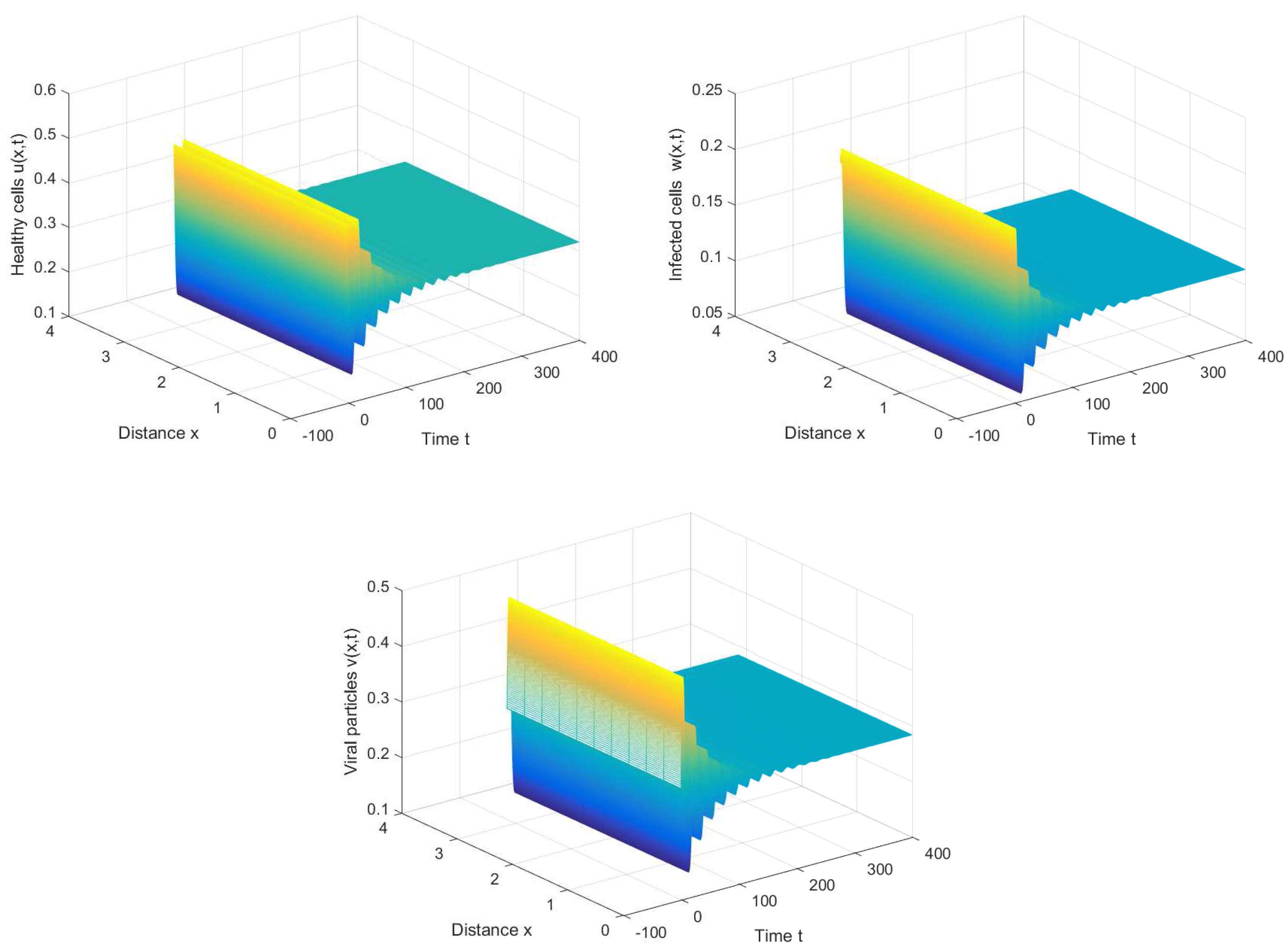
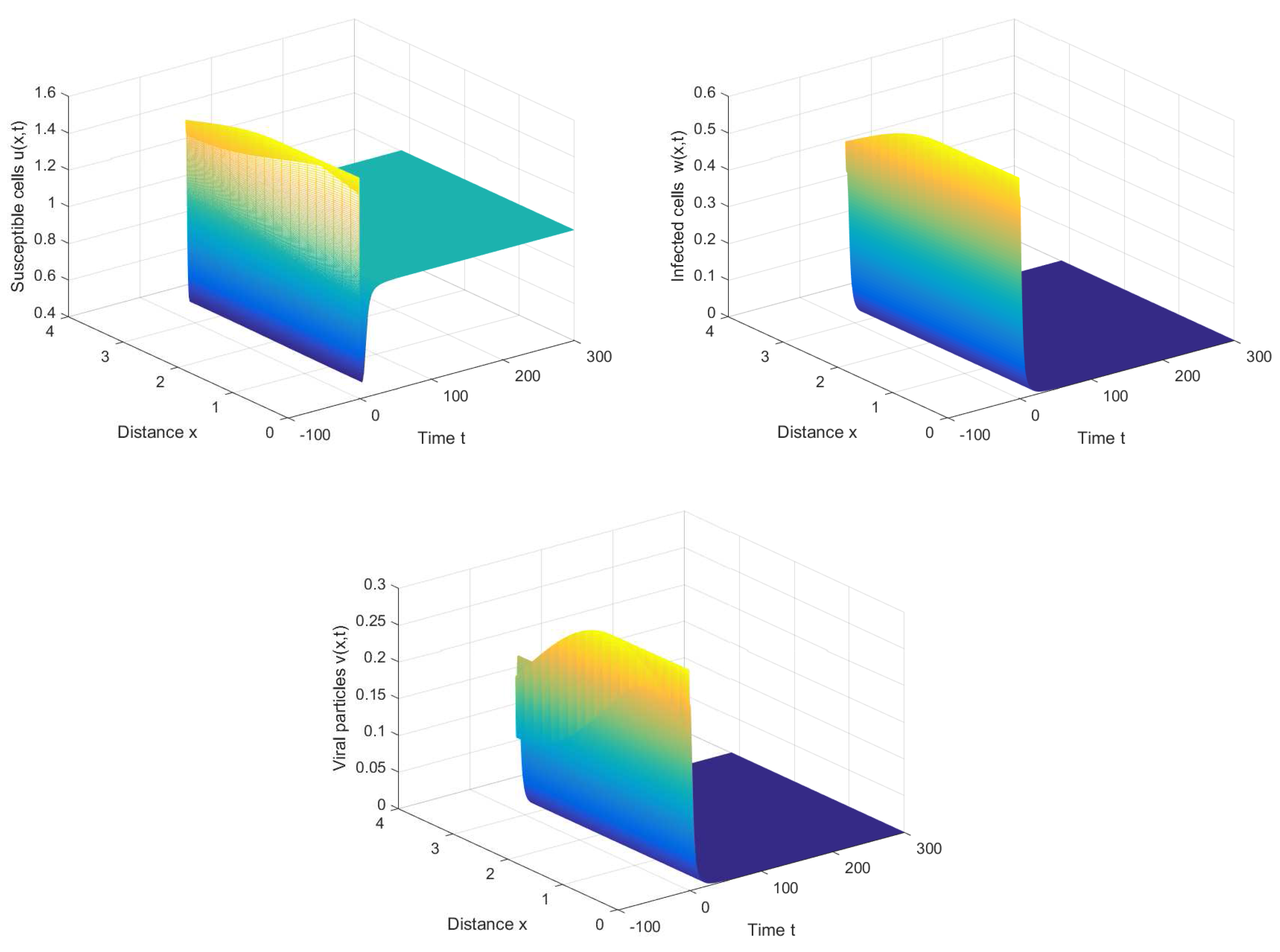
If we choose $k=2.5$, we can obtain the chronic infection equilibrium $E^{*}$ = (0.32, 0.1133, 0.2833). In this case, we can obtain the first critical value ${\tau }_0^{*}=2.5667$. The positive equilibrium $E^{*}$ is asymptotically stable when $\tau <2.5667$ and unstable when $\tau >2.5667$ (see Figure 2 and Figure 3). It is noted that the periodic solution will bifurcate from the positive equilibrium $E^{*}$ when $\tau >2.5667$. Nevertheless, Figure 1 in [30] manifests that the chronic infection equilibrium $E^{*}$ is asymptotically stable when $r=0.5$, $k=2.5$ and $a=0.8$ without spatial diffusion and time delay. The comparison certifies that spatial diffusion and time delay may affect the stability of the system, even leading to instability and oscillation.

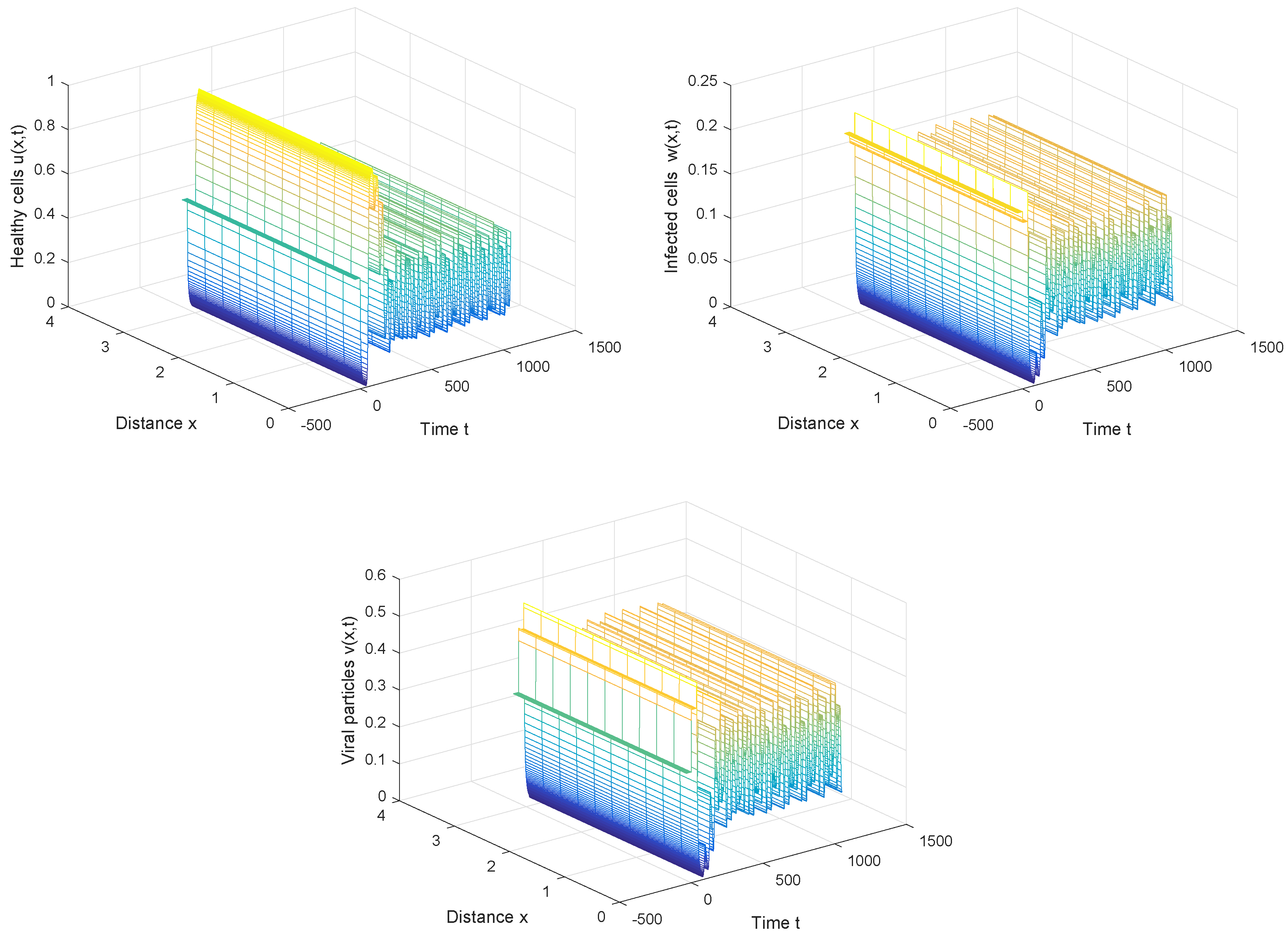
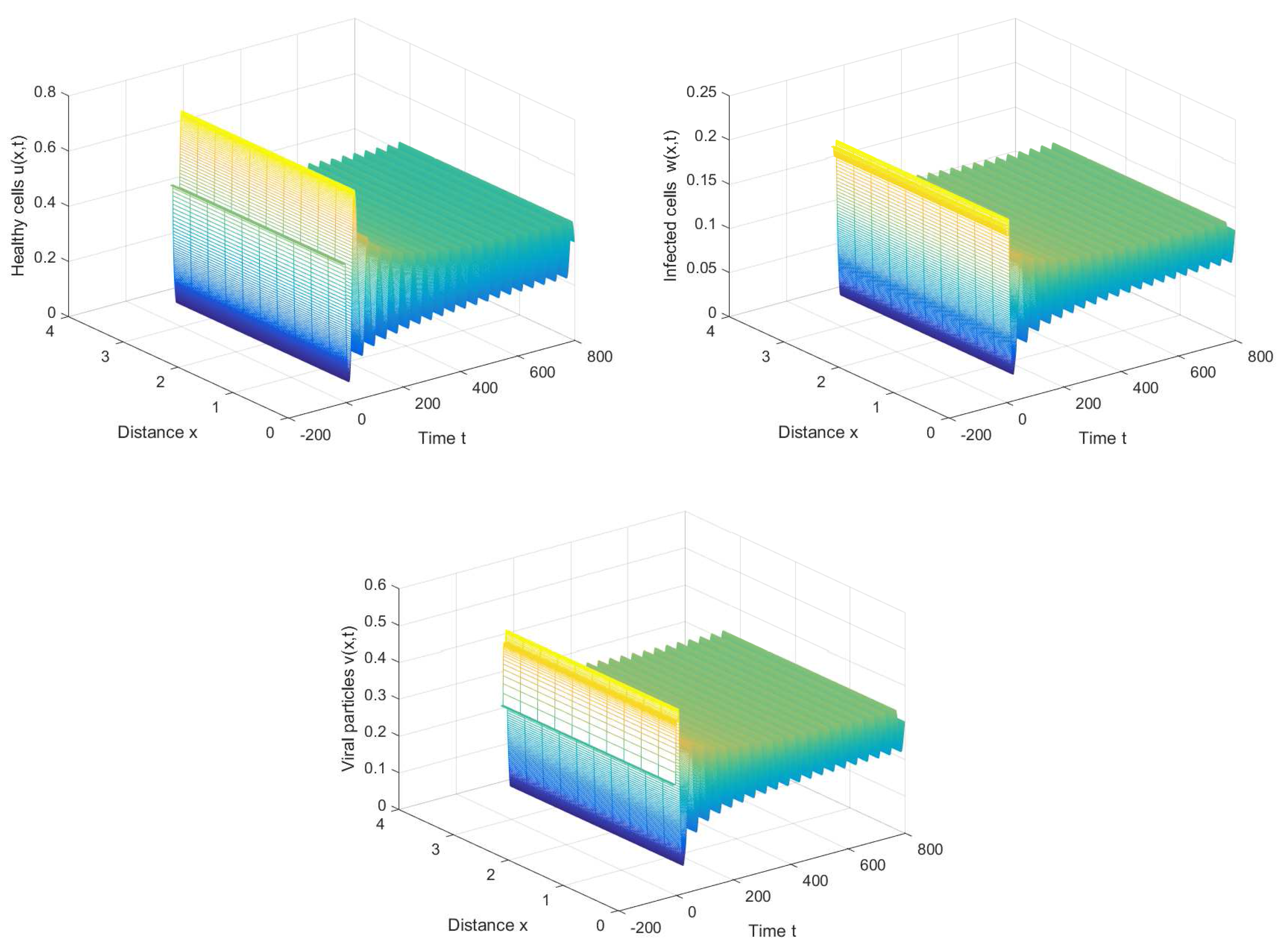
From Figure 4, we can also discover that the periodic solution still exists even when the time delay τ is much greater than the first Hopf bifurcation value ${\tau }_0^{*}$. It is not hard to conjecture that the Hopf bifurcation obtained in Section 3 is global, which means the bifurcating periodic solutions not only exist in the small neighborhood of the bifurcation value, but also exist when the bifurcation parameter is far away from the critical value.

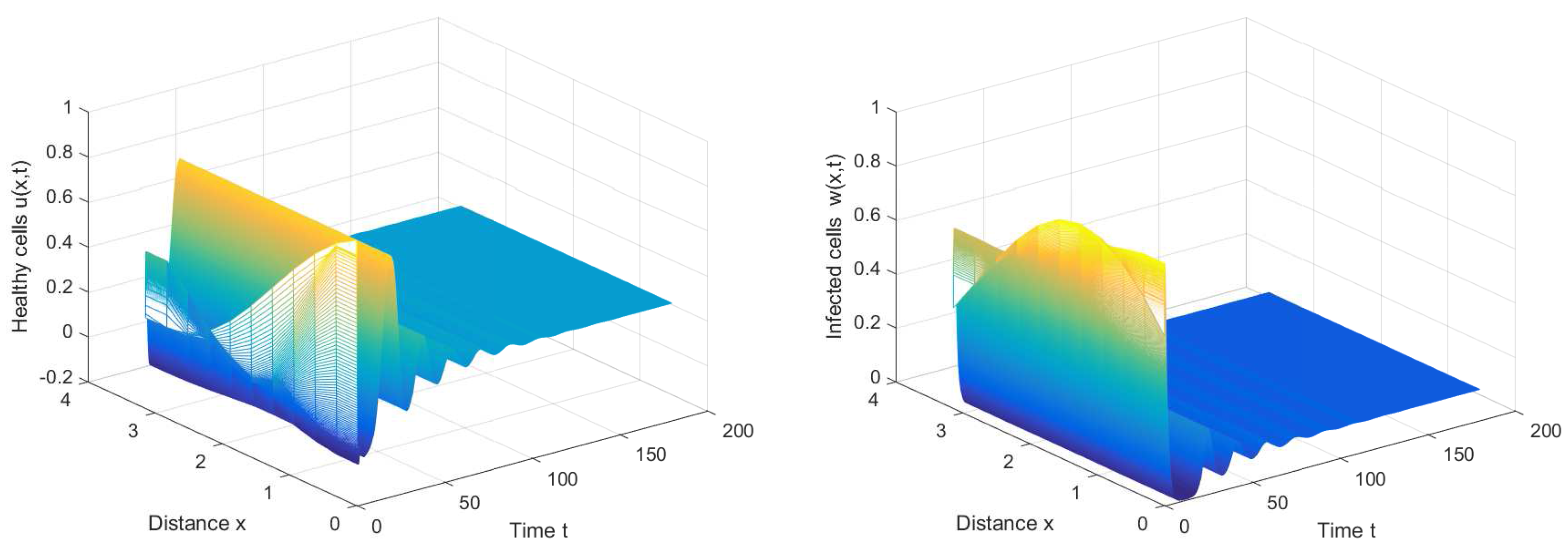
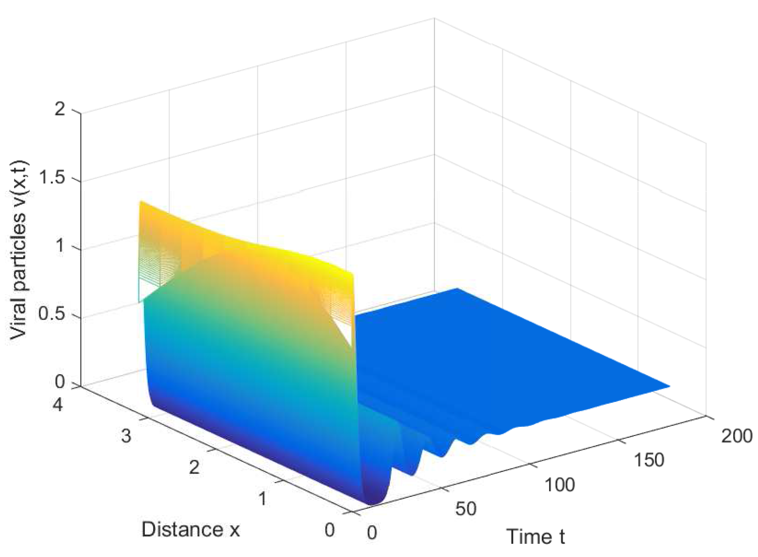
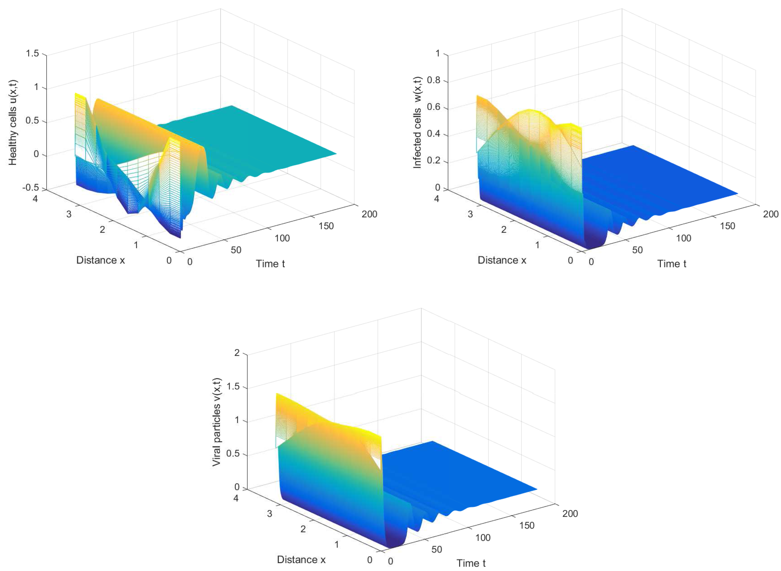
For cross-diffusion System (16), we set $d=1$, $r=0.5$, $k=2.5$ and $a=0.8$. It is observed that the positive equilibrium solution $E^{*}$ is asymptotically stable when $D_{12}=3$ or $D_{12}=10$ with initial conditions $(0.6+0.4sin(x+t),0.5+0.4sin(x+t),1.0+0.6sin(x+t\left)\right)$ (see Figure 5 and Figure 6).

7. Discussion and Conclusions

In this paper, we have developed a delay-diffusion model to investigate the spatiotemporal interactions between the target cells, infected cells and virions. The model here is much more generalized than those in [16,17,30]. Some new dynamic behavior, i.e., time periodic phenomenon, has been generated by spatial diffusion and time delay. This has a guidance function to the viral infection control.

From the analyses in Section 2, we can conclude that the healthy equilibrium may be asymptotically stable when the parameter k is appropriately small for any positive time delay. Biologically, some antiviral drugs may work, and the virus will be eradicated over time.

The results in Section 3 signify the permanence of viral infection whether the positive equilibrium is stable or not. In this case, it is difficult for infected people to fully recover, but some therapeutic schedules still can be chosen to lower the level of virus in the body, making transmission much less likely. For example, to increase the value of parameter a, some biotechnologies may be used to induce the apoptosis of infected cells. It will be necessary to design new drugs to keep the level of virus as low as possible, which is reflected by the decrease of parameter k.

Viral infections in animals provoke an immune response that usually eliminates the infecting virus. Immune responses can also be produced by vaccines. Therefore, it is more legitimate to consider the extended model with immune response. The modified mathematical model consists of at least four reaction-diffusion equations, and the dynamic behaviors will become much more complex. Even so, the study on this model is still necessary and meaningful, and we will leave this for future work.