
Analysis of a Hand-Foot-Mouth Disease Model with Standard Incidence Rate and Estimation for Basic Reproduction Number

School of Mathematics and Physics, Changzhou University, Changzhou 213164, Jiangsu, China
Math. Comput. Appl. 2017, 22(2), 29; https://doi.org/10.3390/mca22020029
Submission received: 8 February 2017
/
Revised: 2 April 2017
/
Accepted: 4 April 2017
/
Published: 8 April 2017
Abstract
:Firstly, an SEIR mathematical model with standard incidence rate is established to describe the transmission of Hand-Foot-Mouth disease (HFMD). The equilibrium of the nondimensionalized model is calculated and the basic reproduction number of the model is defined. In addition, the local stability of the equilibrium is analyzed via the characteristic roots of the Jacobian matrix at the equilibrium, respectively. Numerical simulations are given to confirm the theoretical results. Secondly, a formula aimed to estimate the basic reproduction number of the transmission of HFMD is deduced. As examples to make use of the formula, the basic reproduction number of the HFMD transmission of Singapore of years 2015 and 2016 is estimated based on the newly infected cases notified by the surveillance organizations, respectively. The formula can realize real time estimation for the basic reproduction number and does not need to estimate the transmission efficiency of HFMD between individuals.
1. Introduction
Hand-Foot-Mouth disease (HFMD) is caused by viruses that belong to the enterovirus genus (group), and it is a common disease of early childhood. The group of viruses includes polioviruses, coxsackieviruses, echoviruses and enteroviruses. Among these types of viruses, coxsackievirus A16 (COX A16) and enteroviruses 71 (EV71) are the most common ones to induce HFMD [1]. Since the first HFMD case was reported in New Zealand in 1957, this disease is now endemic worldwide. For example, there are 488,955 cases reported in mainland China in 2008 with an ill-death rate of 0.26/1000; and in 2009, there were 1,155,525 cases reported. Due to the high infectiousness of HFMD, it has been included into the Communicable Surveillance Network of China since 2008 [2].
Mathematical models are now applied to analyze the transmission and control of HFMD aimed to enable a better decision making for health policy makers [1,3,4,5,6,7,8,9,10]. For example, the following HFMD model was constructed in [1]
and the model
was established in [7]. In Models (1) and (2), the variable means the number of the susceptible, the exposed, the infective, the recovered, the quarantined individuals, respectively. The basic reproduction number, the local and global stability of the equilibrium, and the optimal control of Model (1) were analyzed in [1]. We note that only numerical simulations were given in [7] to analyze the transmission of HFMD.
The bilinear incidence rate was adopted in Model (1), while the standard incidence rate was introduced in Model (2). For infectious disease models to describe the transmission among individuals in a heterogeneous environment, the standard incidence rate is more reasonable [11]. Motivated by this, in this paper, we will establish a mathematical model with standard incidence rate to describe the transmission of HFMD diseases, and give the definition of the basic reproduction number of the model. Moreover, we will analyze the local stability of the equilibrium.
The basic reproduction number is related to the severity of communicable diseases. Usually, the disease is more urgent when the disease has a larger basic reproduction number. Different control measures are taken based on the severity of the disease that can be quantified by its basic reproduction number. Hence, the problem of how to estimate the value of the basic reproduction number during the prevalence of a disease with observable data received more and more attention [12,13]. The other aim of this paper is to provide a formula (method) to estimate the value of basic reproduction number of HFMD during its prevalence.
The paper is organized as follows. In Section 2, we give the HFMD transmission model between individuals with standard incidence rate. The basic reproduction number of the model is defined and the stability of the equilibrium of the model is analyzed. Numerical simulations are given to verify the theoretical results. In Section 3, we deduce a formula to estimate the basic reproduction number and further this formula is applied to the transmission of HFMD in Singapore of years 2015 and 2016. Both yearly and real time estimation for the basic reproduction number are estimated. Brief discussions are given in the last section.
2. Mathematical Model and Analysis
2.1. The Model
In this section, we first establish the following model with a standard incidence rate in light of Models (1) and (2)
The biological implications of the parameters and variables of Model (3) are listed in Table 1. With the biological background of Model (3) concerned, it is natural to suppose that all the parameters of Model (3) are positive.
Since , Model (3) can be rewritten as the following model
We further introduce the following transformations of variables>
hence, Model (4) is transformed to the following nondimensionalized model
It is clear that the solutions of Model (5) with nonnegative initial values remain nonnegative for all . Moreover, we define the basic reproduction number of Model (5) as
We have the following results on the existence of equilibrium for Model (5), which can be obtained via direct computation, we omit the details.
Theorem 1.
(i) If , then Model (5) has only a disease free equilibrium which satisfy ; (ii) If , then Model (5) has a positive equilibrium and the disease free equilibrium , where
2.2. Local Stability Analysis
In this part, we will analyze the local asymptotical stability of the disease free equilibrium and the positive equilibrium E* of Model (5). The method used is to analyze the sign of the real parts of characteristic roots of the Jacobian matrix at the corresponding equilibrium. If the real parts of all the characteristic roots of the Jacobian matrix are negative, then the respective equilibrium is locally asymptotically stable; if there is a characteristic root of the Jacobian matrix that has positive real part, then the respect equilibrium is not stable [1]. To obtain the sign of the characteristic roots of a matrix, the Routh-Hurwitz criteria are often applied [11].
Denote the right side of each equation of Model (5) as , respectively. The Jacobian matrix of Model (5) is as follows
Theorem 2.
If , then the disease free equilibrium is locally asymptotically stable; If , then the disease free equilibrium is unstable.
Proof.
In view of Equation (8), the Jacobian matrix, J(), at the disease free equilibrium is
Hence, the characteristic equation of is
where I is the unity matrix. From Equation (9), it is clear that the two characteristic roots of is , , that are both negative. The other two characteristic roots are determined by the following equation
If we denote the two roots of (10) as , , respectively, then
From Equation (6), the definition of , we have provided that . Thus, the real parts of and are both negative. From above, all the roots of Equation (9) have negative real parts if . It follows that the disease free equilibrium is locally asymptotically stable if .
If , then . Consider the function
we have and . Therefore, there is a positive root of . That is, there is characteristic root with positive real part for if , hence, the disease free equilibrium is unstable when . ☐
Theorem 3.
If , then the positive equilibrium of Model (5) is locally asymptotically stable.
Proof.
The Jacobian matrix at the disease free equilibrium is
which follows
where
and , are given in Equation (7).
Noting that
it is consequent that . Further, can also be verified directly. In fact,
Hence, all the solutions of (13) have negative real parts by the Routh-Hurwitz criteria. Thus, is locally asymptotically stable. ☐
2.3. Numerical Simulation of Stability
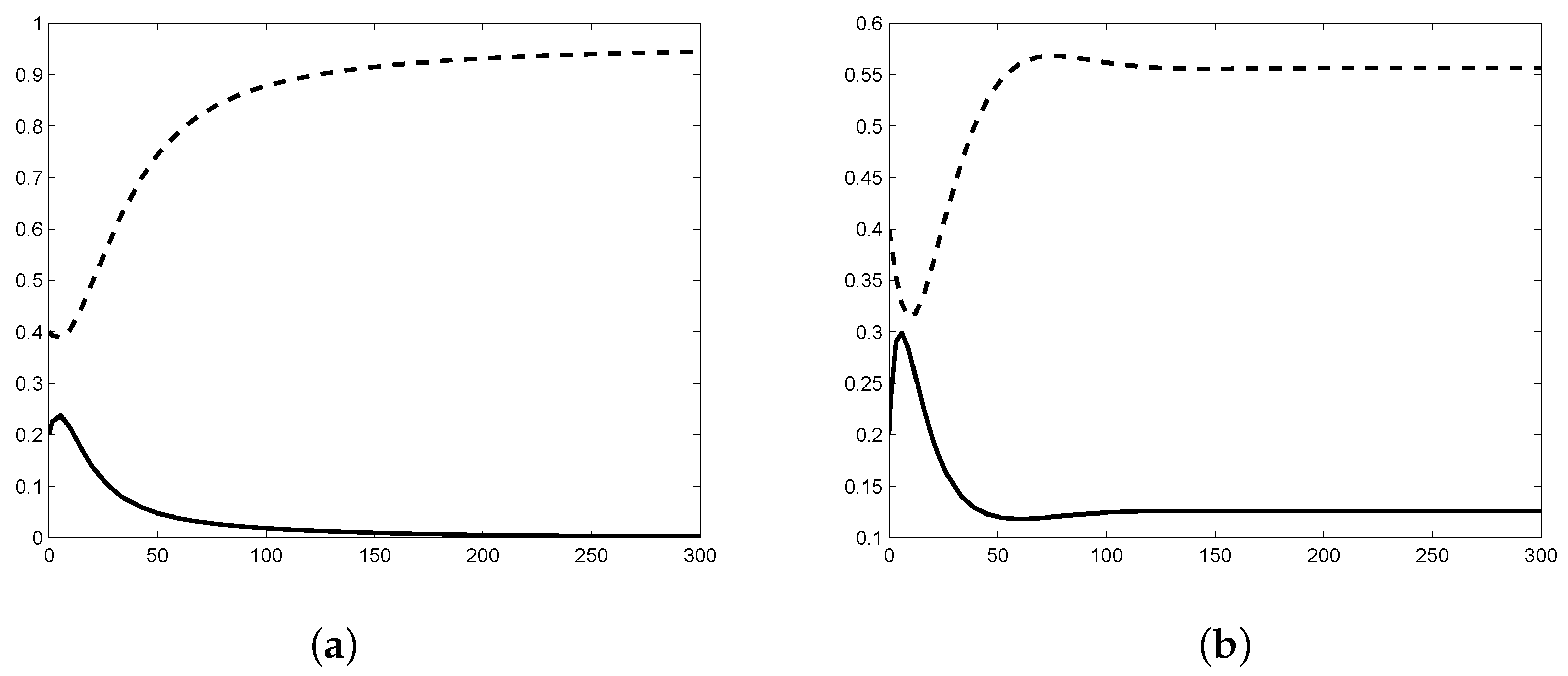
In this part, we give two numerical examples to verify the stability results. Firstly, we set . From Equation (6), we have . Hence, from Theorem 2, the disease free equilibrium of Model (5) is locally asymptotically stable. This can be observed in Figure 1a since the number of the infected individuals tends to 0 as .
3. Estimation of Basic Reproduction Number
3.1. Estimation Formula
In this part, we will derive a formula that can be applied for the estimation of the basic reproduction number with the infected cases periodically notified by the surveillance organizations. We begin with Model (4). Noting that the number of the infected I is much smaller than the total population size N in a region, we set , thus we rewrite the second and the third equation of Model (4) as follows
Further, we suppose the increasing of the accumulation of the exposed and the infected is exponential [14], that is
where is the force of infection and a and b are constants determined by the initial values of E and I. Since Model (14) is linear, is the principal eigenvalue of the matrix
It is direct to verify that one eigenvalue of A is positive and the other one of A is negative when , hence, the value of is given by
and from Equation (6) it can be further written as the following
Thus, from Equation (17) we have
The Equation (18) is the formula can be used for the estimation for the basic reproduction number of the transmission of HFMD during the prevalent stage of the disease. The parameter in Equation (18) can be evaluated via the newly infected cases notified by the surveillance organizations periodically. We add these data to get the accumulation of the infected cases, followed is estimated via curve fitting. The other parameters, , in Equation (18) can be obtained via demographical or pathological statistics.
3.2. Application of the Estimation Formula
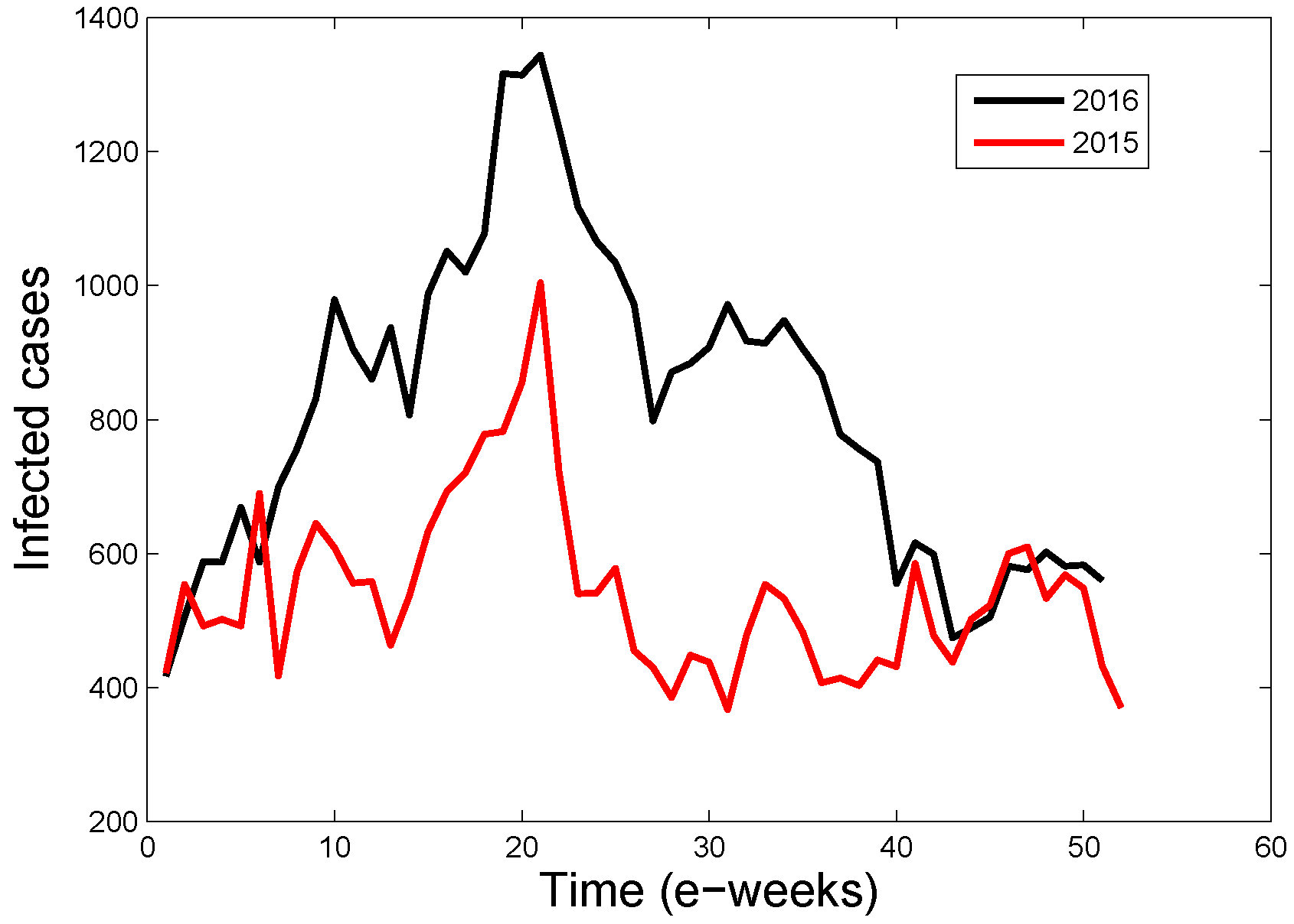
In this part, we give an example to show how to apply Equation (18) to obtain the estimation value of the basic reproduction number of the transmission of HFMD. The newly infected cases of HFMD in Singapore are periodically notified by Ministry of Health of Singapore that can be accessed from the website [15]. The newly infected cases of HFMD of years 2015 and 2016 of each e-weeks (epidemological weeks, consisting of 7 days) are depicted in Figure 2.
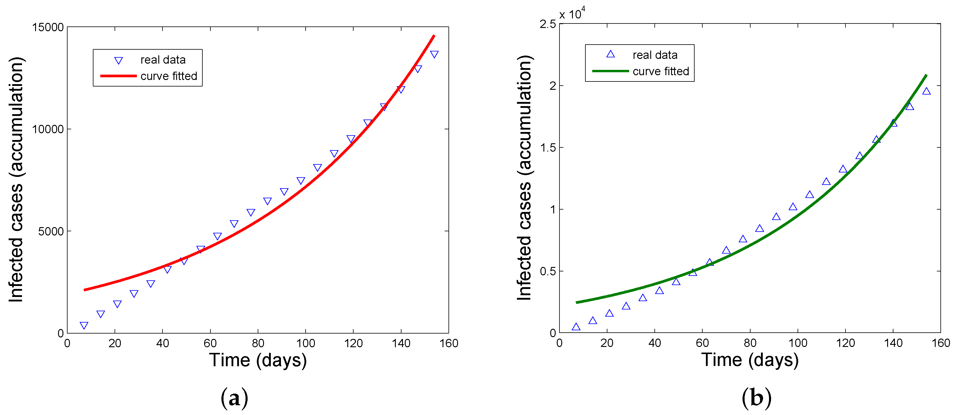
We first show how to estimate the value of in Equation (18). Noting that is the force of infection, which is the exponential increasing rate of the accumulation of the newly infected cases, we add the newly infected cases from the 1st e-week to the e-week of one year, where and m is the last e-week of the year. Thus, we obtain the accumulation vector of the newly infected cases with respect to each e-week of that year consisting of m dimensions. We denote this vector as y. We define an m dimensional vector, , as the time vector whose unit is days. Followed the MATLAB curve fitting toolbox is applied to fit y with respect to x as . Therefore, the value of b is the estimation of . An value is used in MATLAB to show the goodness of the curve fitting. The value of is between 0 and 1 and the curve fitting is better if it merits a larger value. It is clear that the values of and b are different if we apply curve fitting in different time intervals from the 1st e-week to the e-week of one year. Hence we select the value of j that has the largest value in that year and choose the corresponding value of b as the estimation of of that year.
For the transmission of HFMD in Singapore of year 2015, we obtain the largest value of 0.9692 when and the corresponding value of b is 0.1317 (mean value of the 95% Confidence Interval). The curve fitting of y with respect to x from the 1st e-week to the 22nd e-week of year 2015 is depicted in Figure 3a. Thus, the estimation value of in year 2015 is
Similarly, we can also obtain the largest R-square value of 0.9720 when for the transmission of HFMD in Singapore of year 2016. The curve fitting of y with respect to x from the 1st e-week to the 22nd e-week of year 2016 is depicted in Figure 3b. And the estimation value of (mean value of the 95% Confidence Interval) in year 2016 is
Next, we determine the other parameters in Equation (18). The latent period of HFMD is 4–7 days [16]. Thus we set the average latent period as days, that is,
The period for an infected individual to recover from HFMD is 7–10 days [7]. We also set the average recovery period as days, that is,
The life expectancy at birth of Singapore of year 2015 is 82.7 years [17]. Thus, we set
Now the parameters appeared in Equation (18) are all estimated. Substituting Equations (19), (21)–(23) into Equation (18), we obtain that the basic reproduction number of the transmission of HFMD of year 2015 in Singapore is
And from Equations (18), (20)–(23), the basic reproduction number of the transmission of HFMD of year 2016 in Singapore is
3.3. Real Time Estimation of
In Section 3.2, we estimate the basic reproduction number of the transmission of HFMD in Singapore of years 2015 and 2016, respectively. We call this the yearly estimation of . From the estimation process, we know that the basic reproduction number can be estimated till we have the newly infected cases of each e-week in the whole year. However, it is more appropriate to estimate the basic reproduction number of the present e-week with the previous data used, that is, we should estimate the real time basic reproduction number. In this part, we elaborate on this topic.
In Section 3.2, we have supposed that the accumulation of the newly infected cases is exponential increasing (refer to Equation (15)) and they are solutions of the simplified Model (14). Theoretically, the accumulations of the newly infected cases with respect to time are corresponding to the integration of the newly infected cases. Hence, we also suppose that the increasing (or decreasing) of the newly infected cases is exponential since the derivation of the exponential function is still an exponential one. Based on this observation, we can realize the real time estimation of the basic reproduction number.
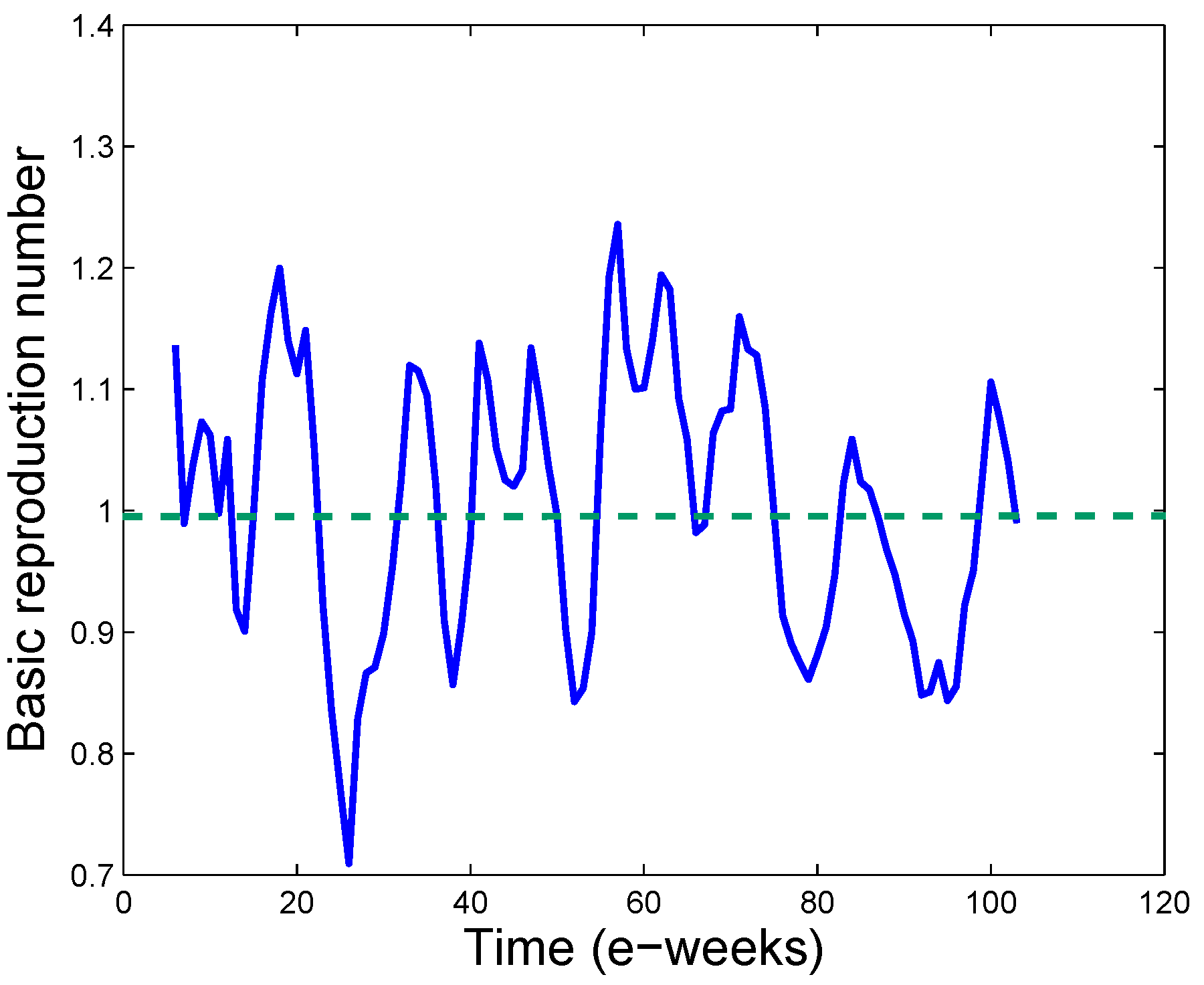
The details to realize the real time estimation is as follows. Suppose that we want to estimate the of the e-week. We collect the newly infected cases, , of the e-week, and denote the data as a vector y. Denote x as the vector since the time unit is days. Followed, we fit y with respect to x as to obtain . Substituting the estimated together with Equations (21)–(23) into Equation (18), we obtain the estimation of the basic reproduction number at the e-week. With this process applied to different h, we obtain the real time estimation of . Figure 4 depicts the variations of of the transmission of HFMD in Singapore of years 2015 and 2016. We note that in Figure 4, we set .
4. Discussion
Mathematical models are now widely applied to analyze the transmission of communicable diseases. The basic reproduction number is the key parameter in theoretical analysis of the models. Usually, the disease free equilibrium is stable when the basic reproduction number is less than 1, and the endemic (positive) equilibrium exists which is stable when the basic reproduction number is larger than 1. In this paper, the HFMD model with standard incidence rate established has been proven to be consistent with this threshold property of the basic reproduction number.
The basic reproduction number is also important in practice. The value of this parameter is related to the severity of the transmission of the infectious diseases, can provide references for the strength of control measures should be taken for health policy makers. Hence, how to estimate the value of the basic reproduction number for communicable disease receives more and more attention by researchers [1,12,13,14,18]. In this paper, we provide a formula to estimate the basic reproduction number both yearly and real time for the transmission of HFMD. And the transmission of HFMD in Singapore of years 2015 and 2016 is as an example to show that the formula can be used in practice. It is estimated that the yearly basic reproduction number of HFMD in Singapore is 1.1924 of year 2015 and 1.2146 of year 2016. Both of them are greater than 1, which implies that HFMD was prevalent in Singapore during these two years.
In Section 3, we take the mean values of the parameters to estimate the basic reproduction number. However, in fact, some parameters in Equation (18) vary their values in intervals. That is, the latent period is 4–7 days, the recovery period is 7–10 days and the 95% Confidence Interval of of year 2015 is [0.01182, 0.01451], of year 2016 is [0.01316, 0.01608]. From Equation (18), we can obtain the yearly basic reproduction number of year 2015 is in the interval [1.1339, 1.2613] and of year 2016 is in the interval [1.1496, 1.2914].
We note that one should estimate the value of to apply Equation (6) directly to estimate the basic reproduction number [1]. The estimation Formula (18) here does not need to estimate the value of . The most urgent need to apply Equation (18) is in the newly-infected cases periodically notified by surveillance organizations.
Acknowledgments
This work was supported by Natural Science Foundation of the Jiangsu Higher Education Institutions of China (No. 15KJB110001) and Natural Science Foundation of China (No. 11501056).
Conflicts of Interest
The author declares no conflict of interest.
References
- Yang, J.Y.; Chen, Y.M.; Zhang, F.Q. Stability analysis and optimal control of a hand-foot-mouth disease (HFMD) model. J. Appl. Math. Comput. 2013, 41, 99–117. [Google Scholar] [CrossRef]
- Zhu, Q.; Hao, Y.T.; Ma, J.Q.; Yu, S.C.; Wang, Y. Surveillance of hand, foot, mouth disease in Mainland China (2008–2009). Biomed. Environ. Sci. 2011, 24, 349–356. [Google Scholar] [PubMed]
- Lai, C.C.; Jiang, D.S.; Wu, H.M.; Chen, H.H. A dynamical model for the outbreaks of hand, foot and mouth diseases in Taiwan. Epidemiol. Infect. 2016, 144, 1500–1511. [Google Scholar] [CrossRef] [PubMed]
- Tinng, F.C.S.; Labadin, J. A Simple Deterministic Model for the Spread of Hand, Foot and Mouth Disease (HFMD) in Sarawak. In Proceedings of the 2008 Second Asia International Conference on Modelling and Simulation, Kuala, Lumpur, 13–15 May 2008; pp. 947–952. [Google Scholar]
- Zhu, Y.; Xu, B.; Lian, X.; Lin, W.; Zhou, Z.; Wang, W. A Hand-Foot-and-Mouth Disease Model with Periodic Transmission Rate in Wenzhou, China. Abstr. Appl. Anal. 2014, 234509. [Google Scholar] [CrossRef]
- Liu, J. Threshold dynamics for a HFMD epidemic model with periodic transmission rate. Nonlinear Dyn. 2011, 64, 89–95. [Google Scholar] [CrossRef]
- Roy, N.; Halder, N. Compartmental modeling of hand, foot and mouth infectious disease (HFMD). Res. J. Appl. Sci. 2010, 5, 177–182. [Google Scholar] [CrossRef]
- Urashima, M.; Shindo, N.; Okabe, M. Seasonal models of herpangina and hand-foot-mouth disease to simulate annual fluctuations in urban warming in Tokyo. Jpn. J. Infect. Dis. 2003, 56, 48–53. [Google Scholar] [PubMed]
- Samanta, G.P. Analysis of a delayed hand-foot-mouth disease epidemic model with pulse vaccination. Syst. Sci. Control Eng. 2014, 2, 61–73. [Google Scholar] [CrossRef]
- Sharma, S.; Samanta, G.P. Analysis of a hand-foot-mouth disease model. Int. J. Biomath. 2017, 10, 1750016. [Google Scholar] [CrossRef]
- Wang, W.D.; Zhou, Y.C.; Lu, Z.Y. Advances in Mathematical Biology; Science Press: Beijing, China, 2008. (In Chinese) [Google Scholar]
- Heesterbeek, J. A brief history of R0 and a recipe for its calculation. Acta Biotheor. 2002, 50, 189–204. [Google Scholar] [CrossRef] [PubMed]
- Hefferman, J.M.; Smith, R.J.; Wahl, L.M. Perspectives on the basic reproductive ratio. J. R. Soc. Interface 2005, 2, 281–293. [Google Scholar] [CrossRef] [PubMed]
- Anderson, R.M.; May, R.M. Infectious Diseases of Human: Dynamics and Control; Oxford University Press: Oxford, UK, 1991. [Google Scholar]
- Ministry of Public Health of Singapore. Available online:https://www.moh.gov.sg/content/moh_web/home/statistics/infectiousDiseasesStatistics/weekly_infectiousdiseasesbulletin.html (accessed on 5 January 2017).
- Samanta, G.P. A delayed hand-foot-mouth disease model with pulse vaccination strategy. Comp. Appl. Math. 2015, 34, 1131–1152. [Google Scholar] [CrossRef]
- Ministry of Public Health of Singapore. Available online:https://www.moh.gov.sg/content/moh_web/home/statistics/Health_Facts_Singapore/Population_And_Vital_Statistics.html (accessed on 5 January 2017).
- Favier, C.; Degallier, N.; Rosa-Freitas, M.G.; Boulanger, J.P.; Costa Lima, J.R.; Luitgards-Moura, J.F.; Menkès, C.E.; Mondet, B.; Oliveira, C.; Weimann, E.T.; et al. Early determination of the reproductive number for vector-borne diseases: The case of dengue in Brazil. Trop. Med. Int. Health 2006, 11, 332–340. [Google Scholar] [CrossRef] [PubMed]
Figure 1.
The dash line is the variation of s, while the solid line is the variation of i. (a) The local stability of the disease free equilibrium when . s tends to 1 and i tends to 0 as ; (b) The local stability of the positive equilibrium when . s tends to and i tends to as .
Figure 1.
The dash line is the variation of s, while the solid line is the variation of i. (a) The local stability of the disease free equilibrium when . s tends to 1 and i tends to 0 as ; (b) The local stability of the positive equilibrium when . s tends to and i tends to as .

Figure 2.
The newly infected cases of years 2015 and 2016 in Singapore notified by Ministry of Health of Singapore. The red line is the variations of the newly infected cases of year 2015, and the black line is that of 2016.
Figure 2.
The newly infected cases of years 2015 and 2016 in Singapore notified by Ministry of Health of Singapore. The red line is the variations of the newly infected cases of year 2015, and the black line is that of 2016.

Figure 3.
The accumulative infected cases fitted by the curve . (a) The year 2015; (b) The year 2016.
Figure 3.
The accumulative infected cases fitted by the curve . (a) The year 2015; (b) The year 2016.

Figure 4.
The real time estimation of the basic reproduction number of hand-foot-mouth disease (HFMD) in Singapore of years 2015 and 2016. The time zone is from the 6th e-week of 2015 to the last e-week of 2016.
Figure 4.
The real time estimation of the basic reproduction number of hand-foot-mouth disease (HFMD) in Singapore of years 2015 and 2016. The time zone is from the 6th e-week of 2015 to the last e-week of 2016.


Table 1.
The biological implications of the parameters and variables of Model (3).
| Parameter or Variable | Biological Implications | Value |
|---|---|---|
| S | number of susceptible individuals | variable |
| E | number of exposed individuals | variable |
| I | number of infective individuals | variable |
| R | number of recovered individuals | variable |
| N | total number of individuals, | variable |
| b | recruitment rate | demographical |
| transmission efficiency rate | estimated | |
| natural death rate | demographical | |
| loss of immunity rate | 0.07 [1,4] | |
| latent duration | estimated | |
| recovery rate | estimated |
© 2017 by the author. Licensee MDPI, Basel, Switzerland. This article is an open access article distributed under the terms and conditions of the Creative Commons Attribution (CC BY) license (http://creativecommons.org/licenses/by/4.0/).
Share and Cite
MDPI and ACS Style
Wu, C. Analysis of a Hand-Foot-Mouth Disease Model with Standard Incidence Rate and Estimation for Basic Reproduction Number. Math. Comput. Appl. 2017, 22, 29. https://doi.org/10.3390/mca22020029
AMA Style
Wu C. Analysis of a Hand-Foot-Mouth Disease Model with Standard Incidence Rate and Estimation for Basic Reproduction Number. Mathematical and Computational Applications. 2017; 22(2):29. https://doi.org/10.3390/mca22020029
Chicago/Turabian StyleWu, Chunqing. 2017. "Analysis of a Hand-Foot-Mouth Disease Model with Standard Incidence Rate and Estimation for Basic Reproduction Number" Mathematical and Computational Applications 22, no. 2: 29. https://doi.org/10.3390/mca22020029