A Family of 5-Point Nonlinear Ternary Interpolating Subdivision Schemes with C² Smoothness

Abstract

The occurrence of the Gibbs phenomenon near irregular initial data points is a widely known fact in curve generation by interpolating subdivision schemes. In this article, we propose a family of 5-point nonlinear ternary interpolating subdivision schemes. We provide the convergence analysis and prove that this family of subdivision schemes is $C^2$ continuous. Numerical results are presented to show that nonlinear schemes reduce the Gibbs phenomenon significantly while keeping the same order of smoothness.

1. Introduction

Subdivision schemes have become very important tools to generate smooth curves and surfaces from initial data points. There are two main categories of subdivision schemes: interpolating subdivision schemes and approximating subdivision schemes. In interpolating subdivision schemes, the initial or existing data points are kept intact and additional data points are inserted in-between at each level of subdivision. On the other hand, in approximating subdivision schemes existing points are replaced by their approximations and new points are inserted between them at each level of refinement. This makes approximating schemes smoother than interpolating subdivision schemes. However, the limiting curve for approximating schemes does not pass through the given initial data points, especially at and near larger jumps or discontinuities. Curves generated by interpolating subdivision schemes pass through the given initial data points but produce oscillations also known as the Gibbs phenomenon near the points with large jumps or discontinuities. These jumps are not desirable for some applications.

Nonlinear subdivision schemes like ENO, WENO, PPH and PCHIP [1,2,3,4,5,6,7,8,9], were introduced during last several years to address Gibbs phenomenon. The arithmetic mean of second differences was replaced by their harmonic mean in a linear subdivision scheme to change it to a nonlinear scheme in [1,2]. The geometric mean of first differences was used instead of the arithmetic mean of first differences in [4]. In this article, we propose a family of 5-point nonlinear ternary interpolating subdivision schemes by replacing the arithmetic mean of third differences with the modified geometric mean of third difference and prove that this family of subdivision schemes is $C^2$ continuous.

We have arranged this article in the following fashion. In Section 2, preliminary concepts and their properties along with some basic terminology are discussed, in Section 3, nonlinear interpolating subdivision schemes are introduced. Convergence analysis of these schemes is provided in Section 4 and some numerical results are presented in Section 5.

2. Preliminaries

A general form of $(2n-1)$-points linear univariate ternary interpolating subdivision scheme S which maps set of data points $f^k={\{f_i^k\}}_{i\in Z}$ into the next refinement level of data points $f^{k+1}={\{f_i^{k+1}\}}_{i\in Z}$ is defined as

$$\begin{array}{c}{\displaystyle f_{3i-1}^{k+1}=\sum _{j=-(n-1)}^{n-1}{a}_j{f}_{i+j}^k,}\hfill \\ f_{3i}^{k+1}=f_i^k,\hfill \\ {\displaystyle f_{3i+1}^{k+1}=\sum _{j=-(n-1)}^{n-1}{a}_{-j}{f}_{i+j}^k.}\hfill \end{array}$$

(1)

The above equation can also be expressed as $f^{k+1}=S(f^k)$. A necessary condition for the uniform convergence of the ternary interpolating subdivision scheme (1) given by [10] is

$${\displaystyle \sum _{j=-(n-1)}^{n-1}{a}_j=\sum _{j=-(n-1)}^{n-1}{a}_{-j}=1.}$$

(2)

For $(x,y)\in R^2$, we define a nonlinear function called the Modified Geometric Mean or MGM as

$$MGM(x,y)=\left\{\begin{array}{ccc}\hfill sign(x)\sqrt{xy}& \mathrm{if}& xy>0\hfill \\ \hfill 0& \mathrm{if}& xy\le 0,\hfill \end{array}\right.$$

(3)

where $sign(x)=1$ if $x\ge 0$ and $sign(x)=-1$ if $x<0$. Nonlinear function MGM defined above has several interesting properties like,

$$MGM(x,y)=MGM(y,x).$$

(4)

$$MGM(-x,-y)=-MGM(x,y).$$

(5)

$$|MGM(x,y)|\le max(|x|,|y|).$$

(6)

$$|AM(x,y)-MGM(x,y)|\le |AM(x,y)|\le max(|x|,|y|)$$

(7)

where $AM(x,y)=\frac{x+y}{2}$.

We recall $PPH$ function $(x,y)\in R^2$ defined by [1,2] as

$$PPH(x,y)=\left\{\begin{array}{ccc}\hfill (1+sign(xy))\frac{xy}{x+y}& \mathrm{for}& xy>0\hfill \\ \hfill 0& \mathrm{if}& xy\le 0.\hfill \end{array}\right.$$

(8)

$PPH$ function defined above also satisfy the properties in (4)–(7).

3. 5-Point Nonlinear Ternary Interpolating Subdivision Schemes

In this section, we construct a class of 5-point nonlinear interpolating subdivision schemes. We start with a well known linear 5-point ternary interpolating subdivision scheme $f^{k+1}=S(f^k)$.

$$\begin{array}{c}{f}_{3i-1}^{k+1}=(w-\frac{4}{81})f_{i-2}^k+(-4w+\frac{10}{27})f_{i-1}^k+(6w+\frac{20}{27})f_i^k+(-4w-\frac{5}{81})f_{i+1}^k+w{f}_{i+2}^k,\hfill \\ f_{3i}^{k+1}=f_i^k,\hfill \\ f_{3i+1}^{k+1}=w{f}_{i-2}^k+(-4w-\frac{5}{81})f_{i-1}^k+(6w+\frac{20}{27})f_i^k+(-4w+\frac{10}{27})f_{i+1}^k+(w-\frac{4}{81})f_{i+2}^k.\hfill \end{array}$$

(9)

This linear subdivision scheme S is $C^2$ for $\frac{1}{324}<w<\frac{1}{162}$ as proved by Zheng et al [11]. We define $\delta f_i=d^3{f}_i=f_{i+3}-3f_{i+2}+3f_{i+1}-f_i$. The above scheme can be rewritten as

$$\begin{array}{c}{f}_{3i-1}^{k+1}=(-\frac{w}{2}-\frac{5}{162})f_{i-2}^k+(\frac{1}{3}-w)f_{i-1}^k+(6w+\frac{20}{27})f_i^k+(-7w-\frac{2}{81})f_{i+1}^k\hfill \\ +(\frac{5}{2}w-\frac{3}{162})f_{i+2}^k+(\frac{1}{27}-3w)(\frac{\delta f_{i-2}^k+\delta f_{i-1}^k}{2}),\hfill \\ f_{3i}^{k+1}=f_i^k,\hfill \\ f_{3i+1}^{k+1}=(\frac{5}{2}w-\frac{3}{162})f_{i-2}^k+(-7w-\frac{2}{81})f_{i-1}^k+(6w+\frac{20}{27})f_i^k+(\frac{1}{3}-w)f_{i+1}^k\hfill \\ +(-\frac{w}{2}-\frac{5}{162})f_{i+2}^k-(\frac{1}{27}-3w)(\frac{\delta f_{i-2}^k+\delta f_{i-1}^k}{2}).\hfill \end{array}$$

(10)

Replacing the arithmetic mean $AM(\delta f_{i-2}^k,\delta f_{i-1}^k)=\frac{\delta f_{i-2}^k+\delta f_{i-1}^k}{2}$ in Equation (10) by the modified geometric mean $MGM(\delta f_{i-2}^k,\delta f_{i-1}^k)$ as defined in (3), we get a class of nonlinear 5-point ternary interpolating schemes $f^{k+1}=S_{NL}(f^k)$.

$$\begin{array}{c}{f}_{3i-1}^{k+1}=(-\frac{w}{2}-\frac{5}{162})f_{i-2}^k+(\frac{1}{3}-w)f_{i-1}^k+(6w+\frac{20}{27})f_i^k+(-7w-\frac{2}{81})f_{i+1}^k\hfill \\ +(\frac{5}{2}w-\frac{3}{162})f_{i+2}^k+(\frac{1}{27}-3w)MGM(\delta f_{i-2}^k,\delta f_{i-1}^k),\hfill \\ f_{3i}^{k+1}=f_i^k,\hfill \\ f_{3i+1}^{k+1}=(\frac{5}{2}w-\frac{3}{162})f_{i-2}^k+(-7w-\frac{2}{81})f_{i-1}^k+(6w+\frac{20}{27})f_i^k+(\frac{1}{3}-w)f_{i+1}^k\hfill \\ +(-\frac{w}{2}-\frac{5}{162})f_{i+2}^k-(\frac{1}{27}-3w)MGM(\delta f_{i-2}^k,\delta f_{i-1}^k).\hfill \end{array}$$

(11)

Similarly, if we replace the arithmetic mean $\frac{\delta f_{i-2}^k+\delta f_{i-1}^k}{2}$ in Equation (10) by modified harmonic mean also known as the $PPH$ function, $PPH(\delta f_{i-2}^k,\delta f_{i-1}^k)$ as defined in (8), we get another class of nonlinear 5-point ternary interpolating schemes.

$$\begin{array}{c}{f}_{3i-1}^{k+1}=(-\frac{w}{2}-\frac{5}{162})f_{i-2}^k+(\frac{1}{3}-w)f_{i-1}^k+(6w+\frac{20}{27})f_i^k+(-7w-\frac{2}{81})f_{i+1}^k\hfill \\ +(\frac{5}{2}w-\frac{3}{162})f_{i+2}^k+(\frac{1}{27}-3w)PPH(\delta f_{i-2}^k,\delta f_{i-1}^k),\hfill \\ f_{3i}^{k+1}=f_i^k,\hfill \\ f_{3i+1}^{k+1}=(\frac{5}{2}w-\frac{3}{162})f_{i-2}^k+(-7w-\frac{2}{81})f_{i-1}^k+(6w+\frac{20}{27})f_i^k+(\frac{1}{3}-w)f_{i+1}^k\hfill \\ +(-\frac{w}{2}-\frac{5}{162})f_{i+2}^k-(\frac{1}{27}-3w)PPH(\delta f_{i-2}^k,\delta f_{i-1}^k).\hfill \end{array}$$

(12)

4. Convergence Analysis of Nonlinear Subdivision Schemes

Nonlinear schemes (11) can be expressed as

$$\begin{array}{c}{f}_{3i-1}^{k+1}=(-\frac{w}{2}-\frac{5}{162})f_{i-2}^k+(\frac{1}{3}-w)f_{i-1}^k+(6w+\frac{20}{27})f_i^k+(-7w-\frac{2}{81})f_{i+1}^k+(\frac{5}{2}w-\frac{3}{162})f_{i+2}^k\hfill \\ +(\frac{1}{27}-3w)\{MGM(\delta f_{i-2}^k,\delta f_{i-1}^k)+AM(\delta f_{i-2}^k,\delta f_{i-1}^k)-AM(\delta f_{i-2}^k,\delta f_{i-1}^k)\},\hfill \\ f_{3i}^{k+1}=f_i^k,\hfill \\ f_{3i+1}^{k+1}=(\frac{5}{2}w-\frac{3}{162})f_{i-2}^k+(-7w-\frac{2}{81})f_{i-1}^k+(6w+\frac{20}{27})f_i^k+(\frac{1}{3}-w)f_{i+1}^k+(-\frac{w}{2}-\frac{5}{162})f_{i+2}^k\hfill \\ -(\frac{1}{27}-3w)\{MGM(\delta f_{i-2}^k,\delta f_{i-1}^k)+AM(\delta f_{i-2}^k,\delta f_{i-1}^k)-AM(\delta f_{i-2}^k,\delta f_{i-1}^k\}.\hfill \end{array}$$

(13)

By simplifying,

$$\begin{array}{c}{f}_{3i-1}^{k+1}=(w-\frac{4}{81})f_{i-2}^k+(-4w+\frac{10}{27})f_{i-1}^k+(6w+\frac{20}{27})f_i^k+(-4w-\frac{5}{81})f_{i+1}^k+w{f}_{i+2}^k\hfill \\ +(\frac{1}{27}-3w)\{MGM(\delta f_{i-2}^k,\delta f_{i-1}^k)-AM(\delta f_{i-2}^k,\delta f_{i-1}^k)\},\hfill \\ f_{3i}^{k+1}=f_i^k,\hfill \\ f_{3i+1}^{k+1}=w{f}_{i-2}^k+(-4w-\frac{5}{81})f_{i-1}^k+(6w+\frac{20}{27})f_i^k+(-4w+\frac{10}{27})f_{i+1}^k+(w-\frac{4}{81})f_{i+2}^k\hfill \\ -(\frac{1}{27}-3w)\{MGM(\delta f_{i-2}^k,\delta f_{i-1}^k)-AM(\delta f_{i-2}^k,\delta f_{i-1}^k)\}.\hfill \end{array}$$

(14)

In general,

$$f^{k+1}=S_{NL}(f^k)=S(f^k)+F(\delta f^k).$$

(15)

where $S_{NL}$ represents a nonlinear subdivision scheme, S is the linear interpolating subdivision scheme (9), which is $C^2$ continuous for $\frac{1}{324}<w<\frac{1}{162}$, and $F(\delta f^k)$ is given by

$$\begin{array}{c}F{(\delta f^k)}_{3i-1}=(\frac{1}{27}-3w)\{MGM(\delta f_{i-2}^k,\delta f_{i-1}^k)-AM(\delta f_{i-2}^k,\delta f_{i-1}^k)\},\hfill \\ F{(\delta f^k)}_{3i}=0,\hfill \\ F{(\delta f^k)}_{3i+1}=-(\frac{1}{27}-3w)\{MGM(\delta f_{i-2}^k,\delta f_{i-1}^k)-AM(\delta f_{i-2}^k,\delta f_{i-1}^k)\}.\hfill \end{array}$$

(16)

Proposition 1.

The subdivision scheme S defined in (9) satisfies the following inequalities.

1. 

$|\delta S{(f^k)}_{3i-1}|\le (\frac{11}{81}-8w)||\delta f^k{||}_{\infty }$ for $0<w<\frac{1}{81}$,

2. 

$|\delta S{(f^k)}_{3i}|\le (\frac{3}{81}+12w)||\delta f^k{||}_{\infty }$ for $w>0$,

3. 

$|\delta S{(f^k)}_{3i+1}|\le (\frac{11}{81}-8w)||\delta f^k{||}_{\infty }$ for $0<w<\frac{1}{81}$.

Proof. 

Consider

$$\delta S{(f^k)}_{3i-1}=\delta f_{3i-1}^{k+1}=f_{3i+2}^{k+1}-3f_{3i+1}^{k+1}+3f_{3i}^{k+1}-f_{3i-1}^{k+1}$$

By using the definition of subdivision scheme S given in (9), we get,

$$\begin{array}{c}\delta S{(f^k)}_{3i-1}=(\frac{4}{81}-4w)f_{i-2}^k+(17w-\frac{19}{81})f_{i-1}^k+(\frac{33}{81}-28w)f_i^k\hfill \\ +(22w-\frac{25}{81})f_{i+1}^k+(\frac{7}{81}-8w)f_{i+2}^k+w{f}_{i+3}^k.\hfill \end{array}$$

(17)

which simplifies to

$$\delta S{(f^k)}_{3i-1}=(4w-\frac{4}{81})\delta f_{i-2}^k+(\frac{7}{81}-5w)\delta f_{i-1}^k+w\delta f_i^k.$$

For $0<w<\frac{1}{81}$, above equation gives,

$$|\delta S{(f^k)}_{3i-1}|\le (\frac{4}{81}-4w)|\delta f_{i-2}^k|+(\frac{7}{81}-5w)|\delta f_{i-1}^k|+w|\delta f_i^k|$$

$$\begin{array}{c}|\delta S{(f^k)}_{3i-1}|\le (\frac{11}{81}-8w)\underset{j}{max}\{|\delta f_j^k|\}=(\frac{11}{81}-8w)||\delta f^k{||}_{\infty }.\hfill \end{array}$$

(18)

which proves the first inequality of Proposition 1. For the second inequality, consider,

$$\delta S{(f^k)}_{3i}=\delta f_{3i}^{k+1}=f_{3i+3}^{k+1}-3f_{3i+2}^{k+1}+3f_{3i+1}^{k+1}-f_{3i}^{k+1}$$

Using the subdivision scheme S in (9) and simplifying, we get,

$$\begin{array}{c}\delta S{(f^k)}_{3i}=3w{f}_{i-2}^k+(-15w-\frac{3}{81})f_{i-1}^k+(30w+\frac{9}{81})f_i^k\hfill \\ +(-30w-\frac{9}{81})f_{i+1}^k+(15w+\frac{3}{81})f_{i+2}^k-3w{f}_{i+3}^k.\hfill \end{array}$$

(19)

$$\delta S{(f^k)}_{3i}=-3w\delta f_{i-2}^k+(6w+\frac{3}{81})\delta f_{i-1}^k-3w\delta f_i^k$$

$$|\delta S{(f^k)}_{3i}|\le |-3w||\delta f_{i-2}^k|+|6w+\frac{3}{81}||\delta f_{i-1}^k|+|3w||\delta f_i^k|$$

For $w>0$, we have,

$$|\delta S{(f^k)}_{3i}|\le (12w+\frac{3}{81})\underset{j}{max}\{|\delta f_j^k|\}=(12w+\frac{3}{81})||\delta f^k{||}_{\infty }.$$

(20)

Similarly, for the third inequality, consider,

$$\delta S{(f^k)}_{3i+1}=\delta f_{3i+1}^{k+1}=f_{3i+4}^{k+1}-3f_{3i+3}^{k+1}+3f_{3i+2}^{k+1}-f_{3i+1}^{k+1}$$

Again, using the definition of the subdivision scheme S in (9) and simplifying, we get,

$$\begin{array}{c}\delta S{(f^k)}_{3i+1}=-w{f}_{i-2}^k+(8w-\frac{7}{81})f_{i-1}^k+(-22w+\frac{25}{81})f_i^k\hfill \\ +(28w-\frac{33}{81})f_{i+1}^k+(-17w+\frac{19}{81})f_{i+2}^k+(4w-\frac{4}{81})f_{i+3}^k\hfill \end{array}$$

(21)

$$\delta S{(f^k)}_{3i+1}=w\delta f_{i-2}^k+(\frac{7}{81}-5w)\delta f_{i-1}^k+(4w-\frac{4}{81})\delta f_i^k$$

For $0<w<\frac{1}{81}$, we get,

$$|\delta S{(f^k)}_{3i+1}|\le (\frac{11}{81}-8w)||\delta f^k{||}_{\infty }.$$

(22)

 ☐

Proposition 2.

Function F defined in (16) satisfies the following inequalities.

1. 

$|\delta F{(\delta f^k)}_{3i-1}|\le 3(\frac{1}{27}-3w)||\delta f^k{||}_{\infty }$, for $0<w<\frac{1}{81}$,

2. 

$|\delta F{(\delta f^k)}_{3i}|\le 6(\frac{1}{27}-3w)||\delta f^k{||}_{\infty }$, for $0<w<\frac{1}{81}$,

3. 

$|\delta F{(\delta f^k)}_{3i+1}|\le 3(\frac{1}{27}-3w)||\delta f^k{||}_{\infty }$, for $0<w<\frac{1}{81}$.

Proof. 

Since

$$\delta F{(\delta f^k)}_{3i-1}=F{(\delta f^k)}_{3i+2}-3F{(\delta f^k)}_{3i+1}+3F{(\delta f^k)}_{3i}-F{(\delta f^k)}_{3i-1}$$

therefore,

$$\begin{array}{c}\delta F{(\delta f^k)}_{3i-1}=(\frac{1}{27}-3w)\{MGM(\delta f_{i-1}^k,\delta f_i^k)-AM(\delta f_{i-1}^k,\delta f_i^k)+3MGM(\delta f_{i-2}^k,\delta f_{i-1}^k)\hfill \\ -3AM(\delta f_{i-2}^k,\delta f_{i-1}^k)+0-MGM(\delta f_{i-2}^k,\delta f_{i-1}^k)+AM(\delta f_{i-2}^k,\delta f_{i-1}^k)\}\hfill \end{array}$$

(23)

$$\begin{array}{c}\delta F{(\delta f^k)}_{3i-1}=(\frac{1}{27}-3w)\{MGM(\delta f_{i-1}^k,\delta f_i^k)-AM(\delta f_{i-1}^k,\delta f_i^k)\}\hfill \\ +2(\frac{1}{27}-3w)\{MGM(\delta f_{i-2}^k,\delta f_{i-1}^k)-AM(\delta f_{i-2}^k,\delta f_{i-1}^k)\}\hfill \end{array}$$

(24)

By Equation (7),

$$|MGM(\delta f_{i-1}^k,\delta f_i^k)-AM(\delta f_{i-1}^k,\delta f_i^k)|\le max\{|\delta f_{i-1}^k|,|\delta f_i^k|\}\le ||\delta f^k{||}_{\infty }$$

and

$$|MGM(\delta f_{i-2}^k,\delta f_{i-1}^k)-AM(\delta f_{i-2}^k,\delta f_{i-1}^k)|\le max\{|\delta f_{i-2}^k|,|\delta f_{i-1}^k|\}\le ||\delta f^k{||}_{\infty }.$$

For $0<w<\frac{1}{81}$, Equation (24) gives

$$|\delta F{(\delta f^k)}_{3i-1}|\le 3(\frac{1}{27}-3w)||\delta f^k{||}_{\infty }.$$

(25)

Proofs of other two inequalities in Proposition 2 are very similar and straight forward. ☐

To prove the convergence of nonlinear scheme $S_{NL}$, we recall the following result from [1,2,3].

Theorem 1.

For F, S and δ given in (15) if $\exists M>0$ such that $\forall g\in l^{\infty }(Z)$

$${||F(g)||}_{\infty }\le {M||g||}_{\infty },$$

(26)

and ∃$c<1$ such that

$$||\delta S(f)+{\delta F(\delta f)||}_{\infty }\le {c||\delta f||}_{\infty },$$

(27)

then the subdivision scheme $S_{NL}$ is uniformally convergent. Moreover, if S is $C^{\alpha }$ convergent then, for all sequence $f\in l^{\infty }(Z)$, $S_{NL}^{\infty }(f)$ is at least $C^{\beta }$ with $\beta =min(\alpha ,-{log}_2(c))$.

Since ternary subdivision has three different formulas at points $3i-1$, $3i$, & $3i+1$, in order to prove conditions (26) and (27) of Theorem 1 for our nonlinear schemes, we have to consider each of them separately.

Case 1: At the point $3i-1$:

$$|\delta S{(f^k)}_{3i-1}+\delta F{(\delta f^k)}_{3i-1}|\le |\delta S{(f^k)}_{3i-1}|+|\delta F{(\delta f^k)}_{3i-1}|$$

By Proposition 1 (part 1) and Proposition 2 (part 1), for $0<w<\frac{1}{81}$, we get,

$$|\delta S{(f^k)}_{3i-1}+\delta F{(\delta f^k)}_{3i-1}|\le (\frac{11}{81}-8w)||\delta f^k{||}_{\infty }+3(\frac{1}{27}-3w)||\delta f^k{||}_{\infty }.$$

$$|\delta S{(f^k)}_{3i-1}+\delta F{(\delta f^k)}_{3i-1}|\le (\frac{20}{81}-17w)||\delta f^k{||}_{\infty }for0<w<\frac{1}{81}.$$

(28)

Case 2: At the point $3i$:

$$|\delta S{(f^k)}_{3i}+\delta F{(\delta f^k)}_{3i}|\le |\delta S{(f^k)}_{3i}|+|\delta F{(\delta f^k)}_{3i}|$$

By Proposition 1 (part 2) and Proposition 2 (part 2), for $0<w<\frac{1}{81}$, we get,

$$|\delta S{(f^k)}_{3i}+\delta F{(\delta f^k)}_{3i}|\le (\frac{3}{81}+12w)||\delta f^k{||}_{\infty }+6(\frac{1}{27}-3w)||\delta f^k{||}_{\infty }.$$

$$|\delta S{(f^k)}_{3i}+\delta F{(\delta f^k)}_{3i}|\le (\frac{7}{27}-6w)||\delta f^k{||}_{\infty }for0<w<\frac{1}{81}.$$

(29)

Case 3: At the point $3i+1$:

$$|\delta S{(f^k)}_{3i+1}+\delta F{(\delta f^k)}_{3i+1}|\le |\delta S{(f^k)}_{3i+1}|+|\delta F{(\delta f^k)}_{3i+1}|$$

By Proposition 1 (part 3) and Proposition 2 (part 3), for $0<w<\frac{1}{81}$, we get,

$$|\delta S{(f^k)}_{3i+1}+\delta F{(\delta f^k)}_{3i+1}|\le (\frac{11}{81}-8w)||\delta f^k{||}_{\infty }+3(\frac{1}{27}-3w)||\delta f^k{||}_{\infty }.$$

$$|\delta S{(f^k)}_{3i+1}+\delta F{(\delta f^k)}_{3i+1}|\le (\frac{20}{81}-17w)||\delta f^k{||}_{\infty }for0<w<\frac{1}{81}.$$

(30)

Let $c=max\{\frac{20}{81}-17w,\frac{7}{27}-6w\}$ then for $0<w<\frac{1}{81}$, we get $c<1$. Therefore, from (28)–(30), we have,

$$||\delta S(f^k)+\delta F(\delta f^k){||}_{\infty }\le c||\delta f^k{||}_{\infty }$$

(31)

for $c<1$ with $0<w<\frac{1}{81}$. Which proves Equation (27).

Now to prove Equation (26), we consider $F(g)$ at $n=3i-1$ as defined in (16), and by using the fact (7), we have,

$${|F(g)}_{3i-1}|\le (\frac{1}{27}-3w){||g||}_{\infty },for0<w<\frac{1}{81}.$$

(32)

At $n=3i$,

$${|F(g)}_{3i}|=0$$

(33)

and similarly, at $n=3i+1$, by using Property (7),

$${|F(g)}_{3i+1}|\le (\frac{1}{27}-3w){||g||}_{\infty },for0<w<\frac{1}{81}.$$

(34)

Let $M=(\frac{1}{27}-3w)$ then $M>0$, for $0<w<\frac{1}{81}$. Therefore, from Equations (32)–(34), we get,

$${||F(g)||}_{\infty }\le {M||g||}_{\infty }.$$

(35)

which proves Equation (26) and consequently proves that our class of 5-point nonlinear ternary interpolating subdivision schemes $S_{NL}$ given in (11) is uniformly convergent for $0<w<\frac{1}{81}$.

It is noted that c as given in (31) can be restricted as $c\le \frac{13}{54}$ for $\frac{1}{324}\le w<\frac{1}{162}$. Which gives $\beta =2$ as defined in Theorem 1 and hence proves that $S_{NL}^{\infty }$ is $C^2$ for $\frac{1}{324}\le w<\frac{1}{162}$.

Since functions $PPH$ and $MGM$ are nonlinear and satisfy properties given in (4)–(7) which we used for $MGM$ to prove the convergence of (11). Therefore, it can easily be verified by replacing $MGM$ function with $PPH$ function in the above proof that subdivision schemes (12) are also $C^2$ continuous.

5. Numerical Results

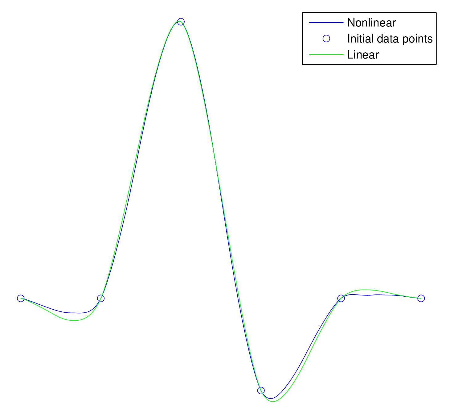
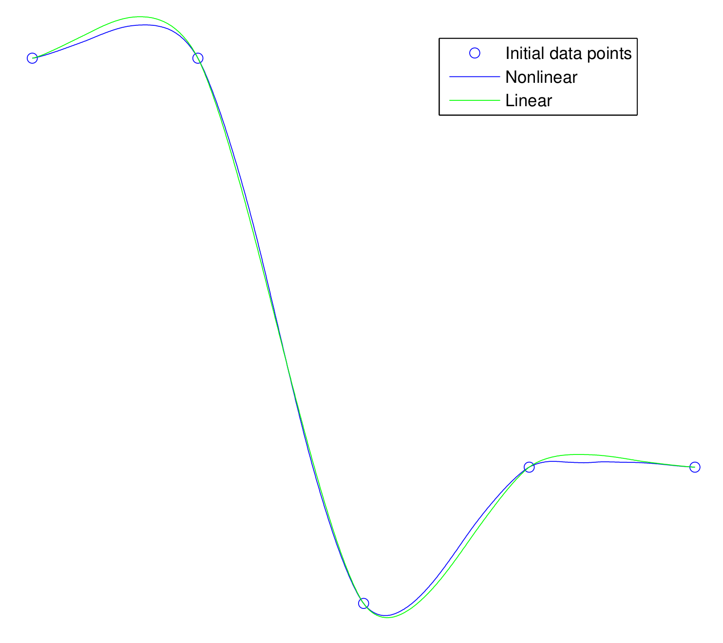
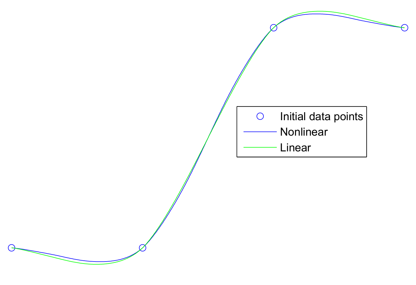
We picked three examples with a varying number of irregularities in initial data points. In Figure 1, two smooth curves are generated from the initial control or data points, one with linear scheme (9) and another with a nonlinear scheme (11) both with $w=1/230$. One can easily see oscillations or Gibbs phenomenon for linear scheme but for the nonlinear scheme it is reduced. Figure 2, shows different initial data points and the corresponding smooth curves: one with the linear scheme (9) and one with nonlinear scheme (11) with $w=1/230$. In Figure 3, initial data points are selected from the step function and the corresponding smooth curves are generated with the linear scheme (9) and nonlinear scheme (11) with $w=1/230$. Improvement is evident. Curves generated from nonlinear schemes reduce the Gibbs phenomenon.

6. Conclusions

In this article, we proposed a class of 5-point nonlinear interpolating subdivision schemes. It is proved that our schemes are at least $C^2$ continuous. Numerical results are presented to show that curves generated by these schemes reduce the Gibbs phenomenon while keeping the same level of smoothness.

References

- Amat, S.; Dadourian, K.; Liandrat, J. On a nonlinear subdivision scheme avoiding Gibbs oscillations and converging towards Cs functions with s > 1. Math. Comput. 2011, 80, 959–971. [Google Scholar] [CrossRef]
- Amat, S.; Dadourian, K.; Liandrat, J. On a nonlinear 4-point ternary and interpolatory multiresolution scheme elimenating the Gibbs phenomenon. Int. J. Numer. Anal. Model. 2010, 7, 261–280. [Google Scholar]
- Arandiga, F.; Donat, R.; Santagueda, M. The PCHIP subdivision scheme. Appl. Math. Comput. 2016, 272, 28–40. [Google Scholar] [CrossRef]
- Aslam, M. C1 continuity of 3-point nonlinear ternary interpolating subdivision schemes. Int. J. Numer. Methods Appl. 2015, 14, 119–132. [Google Scholar]
- Aslam, M.; Abeysinghe, W. Odd-Ary Approximating Subdivision Schemes and RS Strategy for Irregular Dense Initial Data. Available online: http://downloads.hindawi.com/journals/isrn.mathematical.analysis/2012/745096.pdf (accessed on 22 March 2018).
- Aspert, N.; Ebrahimi, T. Non-linear Subdivision of Univariate Signals and Discrete Surfaces. Available online: https://infoscience.epfl.ch/record/33290 (accessed on 22 March 2018).
- Cohen, A.; Dyn, N.; Matei, B. Quasilinear subdivision schemes with applications to ENO interpolation. Appl. Comput. Harmonic Anal. 2003, 15, 89–116. [Google Scholar] [CrossRef]
- Harizanov, S. Stability of Nonlinear Subdivision Schemes and Multiresolutions. Master’s Thesis, Jacobs University, Bremen, Germany, December 2007. [Google Scholar]
- Mustafa, G.; Ghaffar, A.; Aslam, M. A subdivision-regularization framework for preventing over fitting of data by a model. Appl. Appl. Math. Int. J. 2013, 8, 178–190. [Google Scholar]
- Hassan, M.F.; Ivrissimitzis, I.P.; Dodgson, N.A.; Sabin, M.A. An interpolating 4-point C2 ternary stationary subdivision scheme. Comput. Aided Geom. Des. 2002, 19, 1–18. [Google Scholar] [CrossRef]
- Zheng, H.; Hu, M.; Peng, G. Constructing 2n-1-point ternary interpolatory subdivision schemes by using variation of constants. In Proceedings of the International Conference on Computational Intelligence and Software Engineering, Wuhan, China, 11–13 December 2009; pp. 1–4. [Google Scholar]
Figure 1.
Initial control points and curve generated by 5-point linear ternary interpolating subdivison scheme (5th level) in (9) and 5-point nonlinear ternary interpolating subdivision scheme (11) with .
Figure 2.
© 2018 by the author. Licensee MDPI, Basel, Switzerland. This article is an open access article distributed under the terms and conditions of the Creative Commons Attribution (CC BY) license (http://creativecommons.org/licenses/by/4.0/).
Share and Cite
MDPI and ACS Style
Aslam, M. A Family of 5-Point Nonlinear Ternary Interpolating Subdivision Schemes with C2 Smoothness. Math. Comput. Appl. 2018, 23, 18. https://doi.org/10.3390/mca23020018
AMA Style
Aslam M. A Family of 5-Point Nonlinear Ternary Interpolating Subdivision Schemes with C2 Smoothness. Mathematical and Computational Applications. 2018; 23(2):18. https://doi.org/10.3390/mca23020018
Chicago/Turabian StyleAslam, Muhammad. 2018. "A Family of 5-Point Nonlinear Ternary Interpolating Subdivision Schemes with C2 Smoothness" Mathematical and Computational Applications 23, no. 2: 18. https://doi.org/10.3390/mca23020018