Article

How Am I Driving? Using Genetic Programming to Generate Scoring Functions for Urban Driving Behavior

by
Roberto López
1,
Luis Carlos González Gurrola
1,*,
Leonardo Trujillo
2,
Olanda Prieto
1,
Graciela Ramírez
1,
Antonio Posada
2,
Perla Juárez-Smith
2 and
Leticia Méndez
1
1
Facultad de Ingeniería, Universidad Autónoma de Chihuahua, Circuito No. 1, Nuevo Campus Universitario, Apdo. postal 1552, Chihuahua 31240, Mexico
2
Departamento de Ingeniería en Electrónica y Eléctrica, Instituto Tecnológico de Tijuana, Calzada Tecnológico SN, Tomas Aquino, Tijuana 22414, Mexico
*
Author to whom correspondence should be addressed.
Math. Comput. Appl. 2018, 23(2), 19; https://doi.org/10.3390/mca23020019
Submission received: 7 March 2018 / Revised: 27 March 2018 / Accepted: 30 March 2018 / Published: 3 April 2018
(This article belongs to the Special Issue Numerical and Evolutionary Optimization)

Abstract

:
Road traffic injuries are a serious concern in emerging economies. Their death toll and economic impact are shocking, with 9 out of 10 deaths occurring in low or middle-income countries; and road traffic crashes representing 3% of their gross domestic product. One way to mitigate these issues is to develop technology to effectively assist the driver, perhaps making him more aware about how her (his) decisions influence safety. Following this idea, in this paper we evaluate computational models that can score the behavior of a driver based on a risky-safety scale. Potential applications of these models include car rental agencies, insurance companies or transportation service providers. In a previous work, we showed that Genetic Programming (GP) was a successful methodology to evolve mathematical functions with the ability to learn how people subjectively score a road trip. The input to this model was a vector of frequencies of risky maneuvers, which were supposed to be detected in a sensor layer. Moreover, GP was shown, even with statistical significance, to be better than six other Machine Learning strategies, including Neural Networks, Support Vector Regression and a Fuzzy Inference system, among others. A pending task, since then, was to evaluate if a more detailed comparison of different strategies based on GP could improve upon the best GP model. In this work, we evaluate, side by side, scoring functions evolved by three different variants of GP. In the end, the results suggest that two of these strategies are very competitive in terms of accuracy and simplicity, both generating models that could be implemented in current technology that seeks to assist the driver in real-world scenarios.

1. Introduction

It is a well known problem that reckless driving affects society in a variety of ways, with noteworthy impacts on health, economic and social issues. Government offices in charge of planning and deploying urban programs could largely benefit by technological tools which can provide decision-support information to develop appropriate public policies. On their part, taxicab companies or on-line transportation services could also benefit from such tools to optimize resources or reduce economic risks related to insurance or maintenance. At the same time, insurance companies could work on coverage plans designed according to a driver’s profile which could, at least partially, be based on automatic tools that exploit useful information obtained from regular driving trips [1,2].
For these reasons, there has been a growing amount of interest in the development of approaches that can extract information from sensors embedded in almost every modern mobile device, such as GPS, gyroscope, magnetometer and accelerometer. This opens the possibility for a broad spectrum of new applications that exploit different ways of collecting and analyzing sensor data. In particular several works have proposed to transform sensor readings to deliver a driving safety score, with a small but varied set of techniques, such as simple penalty functions [3], fuzzy classifiers [4] or Bayesian models [5]. Moreover, other authors have suggested to expand the amount of sensors used to score driving behaviors, such as using real time data about weather, road conditions and traffic density, among others [6].
The problem of calculating a driving score based on the performance of the driver could be seen as a computational learning task, where given a feature vector that contains the frequency of risky maneuvers the goal is to assign a score to represent the driver’s performance in a risk-safety scale (this problem could also be seen as a machine learning problem for human-rating). Recently, in [7] the authors presented the evaluation of seven different Machine Learning (ML) approaches to learn how individuals assigned a driving score. From this comparison a clear winner emerged, this being the Genetic Programming (GP) approach. Since then, a question that remained open was to evaluate if other variants of GP could attain better results. In this manuscript we approach this question by evaluating three different GP variants that have proved to be successful for a variety of problems, namely GPTIPS [8], neatGP [9] and neat-GP-LS [10]. The first method generates models linear in parameters, the second builds non-linear models using a bloat control mechanism, and the last one extends neat-GP by including a local search operator. Results suggest that GPTIPS as well as neatGP-LS are very competitive at evolving mathematical scoring functions, and given their accuracy and simplicity could be integrated in current car technology to assist the driver.
The rest of the paper is organized as follows. In Section 2 we overview related work on the problem domain. Next, in Section 3 we describe our proposed approach, including building the dataset, posing the learning problem and applying GP to solve it. In Section 4 we detail the results obtained, and finally in Section 5 we present the main conclusions.

2. Related Work

The exponential growth of the world population has increased traffic flow in all cities worldwide. Therefore, new and improved urban policies must be implemented, and the use of current technology is becoming a mandatory requirement to alleviate the social impact of road accidents [11]. Recent works deal with detecting and classifying sensor data from mobile devices, as well as sensors embedded in automobiles [3]. Due to the increase availability of such devices, there is a surge of possible applications for the data gathered by them. Opportunely determining the mental and physical state of a driver through an analysis of their behavior might help mitigate the number of car accidents. For instance the work in [6] details the social impact of traffic accidents in the UK, and approaches the problem via a context-aware architecture that links data from sensors, driver behavior and road infrastructure to jointly help decrease the possibility of road accidents. While most works attempt to distinguish between aggressive from calm driving, drunk and careless driving might also be identified. For example, Dai et al. [12] tried to detect drunk driving through an inexpensive platform using mobile phone sensors, sending notifications to the proper authorities and to the driver.
However, modeling the behavior of a driver is a very complex task, it involves a large number of variables and subjective data. Self perception of driving skills is very biased, some drivers might believe that their driving style is safe, whilst a driving companion may have an entirely different opinion. Detecting aggressive behavior while driving is a problem that has been addressed through several ML techniques, that exploit specific types of sensor data. In a large study presented in [1], a mobile application was designed using a crowd-sourcing approach. Data from sensors embedded in mobile devices was recorded by the application and used in conjunction with automobile characteristics and road conditions. This distributed telematics platform allowed the authors to successfully gather data regarding unsafe behaviors whilst driving. Their approach used a multivariate Gaussian model to determine the likelihood of normal versus abnormal driving maneuvers. The work detailed in [13,14] also deals with classification of unsafe driving practices, from sensor data within mobile phones. The use of such sensors is extremely prevalent due to the deep penetration of the aforementioned devices among current drivers. Most of the works that attempt to detect aggressive or reckless behaviors while driving, focus on accurately detecting specific driving events, like sudden stops, intrusive lane changes or speeding. This is usually done by posing a classification problem. ML approaches that have been used to solve this problem include Fuzzy Logic Systems and Time Series analysis [4,13,15,16,17], to mention two prominent techniques. However, we argue that classifying these events is only the first step towards properly determining unsafe driving behaviors. To properly score a driving trip, one should account for the total frequency of the events with regards to the total length of the trip. The nature of these events are vastly studied under the concept of Insurance Telematics [2], where they are called Figure of Merits (FoMs). Once these FoMs or risky maneuvers are detected, a new regression problem appears, which is related to calculating a driving score. For instance, in the work of [5] the authors attempt to score driving trips using a Bayesian classifier to differentiate between risky and safe maneuvers. In [7], the authors compared a Fuzzy Inference System [1], a Safety Index [13], a Bayesian regressor [5], a Multi-layer perceptron, a Random Forrest, a Support Vector regressor and a GP approach to learn how individuals score 200 virtual road trips, where each trip was represented by a feature vector containing the frequency of risky maneuvers. Results showed that the GP strategy was superior than competitors, even in some cases with statistical significance. We depart from this point, where a main comparison of approaches was already done, positioning GP as the best performer. On top of these results this manuscript compares the performance of three flavors of GP, with the aim to know if a better performance can be found.

3. Methodology

In this section we briefly describe the datasets that will be used. We also present the different flavors of GP that are compared. Finally, we present the performance metric and the statistical test that is used to validate the analysis.

3.1. The Dataset

Given that our aim is to compared GP-strategies on the first place, but also to contextualize our results given prior results, we will use the same dataset employed in [7]. This dataset is composed of 200 virtual trips, where each trip is characterized by a vector of frequencies, with each position of the vector associated to a particular risky maneuver. Each trip (vector) is also associated to a Driving score (target value) that was computed as the mean value of all scores given to it by a group of drivers. The risky maneuvers considered in the vector are analogous to those found in [18], which suggests those types of incidents are closely related to safety on the road. As an example, Table 1 shows how a single road trip was characterized by a human observer based on the frequency of each risky maneuver. To establish the ground truth for the driving score, the descriptive vector of each trip was shown to several human observers (a total of 40) who were then asked to provide a subjective score for the trip on a scale of 1 (very unsafe) to 10 (very safe). This means that each observer imposed subjective criteria when deriving their score, based on what events they considered to be the most correlated with driving safety.
To compare approaches, two experiments were envisioned. In the first experiment, now called 1–10 scale, the dataset was used the way it is, since the target values for all the feature vectors contains a score in the range [1, 10]. For the second experiment, the targets were fitted to a 1–4 scale following the criteria proposed in [3]. Both experiments were planned to analyzed the performance of the approaches in a fine and coarse version of the dataset. Note that, for both scales, the minimum value corresponds to a totally reckless trip, and the highest value to a totally safe trip.

3.2. Genetic Programming and Tested Flavors

GP uses an evolutionary search to derive small programs, operators or models. In most cases, GP is used to solve different kinds of ML tasks, with the most common being symbolic regression, producing Symbolic Regression Models (SRMs). These models represent the relation between the input variables and the dependent output variable. Therefore, in this work the problem is posed as a symbolic regression one, where GP is used to evolve the scoring functions, taking as input each of the frequency features described above. In standard GP, and all the variants used here, the SRMs are represented using a tree structure, where internal nodes contain elements from a set of basic mathematical operations called the function set. Tree leaves contain input values, in this case each of the x i features and random constants. The fitness function used in all cases is the Root Mean Squared Error (RMSE) ( R M S E = 1 n Σ i = 1 n p r e d i t a r g e t i 2 , where t a r g e t i is the score in the survey for the i t h road trip, p r e d i is the predicted score given by a particular scoring function.) between the estimated score given by an individual SRM and the ground truth score on all of the samples in a training set. As for any other evolutionary algorithm, in GP, special genetic operators are used to build new SRMs (offspring) from previous ones (parents) that were chosen stochastically, with a bias that is based on the fitness of the solution. In order to be a self-contained manuscript, the general pseudocode of a GP search is summarized in Algorithm 1. The specific strategies of GP evaluated in this manuscript are described next.
Algorithm 1 Genetic Programming pseudocode.
  1:  for i = 1 to N u m O f G e n e r a t i o n s (or until an acceptable solution is found) do
  2:    if 1st generation then
  3:      generate initial population with primitives (variables, constants and elements from the function set)
  4:    end if
  5:    Calculate fitness (minimize RMSE) of population members
  6:    Select n parents from population (based on fitness)
  7:    Stochastically apply Genetic operators to generate n offspring
  8:  end for
  9:  Return best individual (based on fitness) found during search

3.2.1. GPTIPS V2

GPTIPS implements a multi-gene strategy to represent individuals in the population. Basically, the representation of a single individual includes a collection of trees, and the final SRM is constructed as a linear combination of all the trees. This is a linear in parameter model, with the model weights fitted with linear regression. GPTIPS also uses a multi-objective selection pressure, where model complexity (size) is also included as a selection criterion. A good aspect of the GPTIPS tool is that it offers a variety of post execution reports, such as summary information about the latest generation, the best solutions on the Pareto front, considering both the training and testing partitions, the complexity of the proposed solutions in terms of number of nodes, RMSE and R 2 of the best programs, among other useful stats [8] (http://gptips.sourceforge.net/).

3.2.2. neatGP

The neatGP method [9] combines GP with the NeuroEvolution of Augmenting Topologies algorithm (NEAT) [19]. It was proposed as a bloat-free GP search based on the results obtained by Flat Operator Equalization (Flat-OE) [20]. In general, neatGP preserves a diverse population of individuals of different shapes and sizes, by using speciation techniques and standard fitness sharing. Results on both regression and classification tasks have show that neatGP can produce very accurate models that are orders of magnitude smaller than the ones produced by standard GP [9]. The implementation used in this paper was developed on top of the DEAP Library [21].

3.2.3. neatGP-LS

One way to enhance a global search algorithm or metaheuristic is by embedding additional search operators that can improve the overall exploitation ability of the search process. In particular, GP utilizes search operators that operate at the level of syntax, i.e., they modify the syntactic representation of the programs or SRMs. This can make the search more inefficient when what is required are small steps in the solution space. That is one of the reasons that GPTIPS, for instance, uses linear regression to fit the linear parameters of the evolved models. Similarly, neatGP-LS integrates a local search (LS) mechanism within neatGP, by first parameterizing each solution by adding a real-valued weight θ to each node and fitting those weights using a trust region optimizer [10]. In standard GP these weights are usually ignored and considered to be θ = 1 , in neat-GP this represents their initial value but the numerical optimizer can tune the weights as required. One effect of embedding a LS method within GP is that smaller solutions in the population have a better chance of surviving after the LS is applied, since they are more susceptible to suboptimal parameter values.

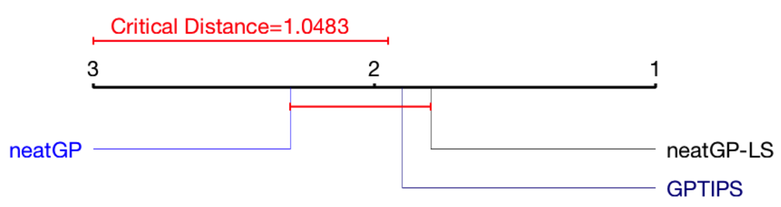
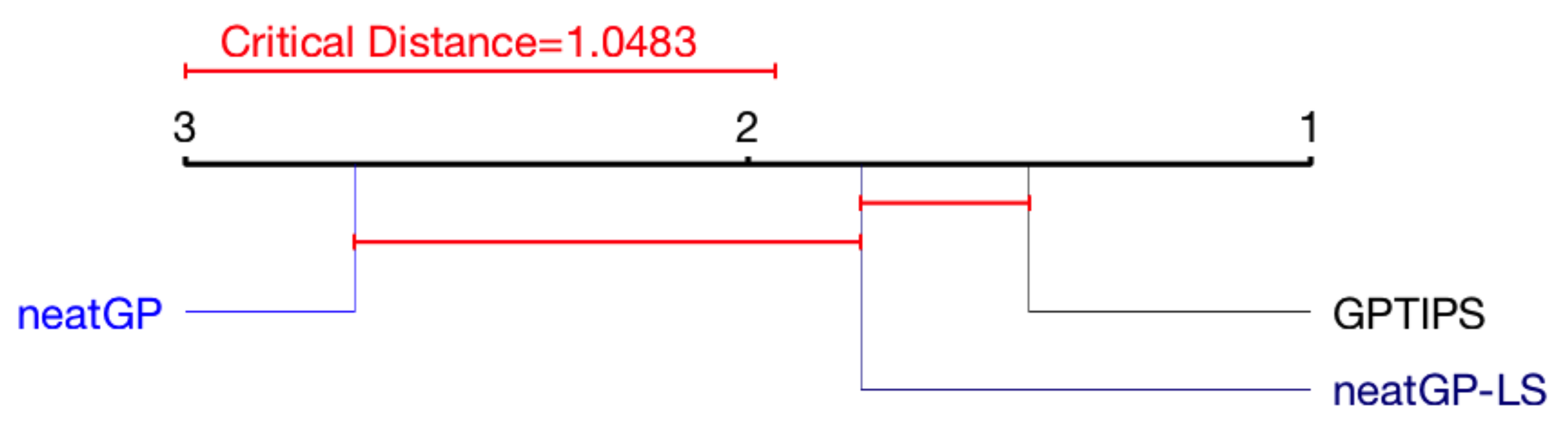
3.3. Statistical Analysis: Friedman Test and Critical Difference Diagram
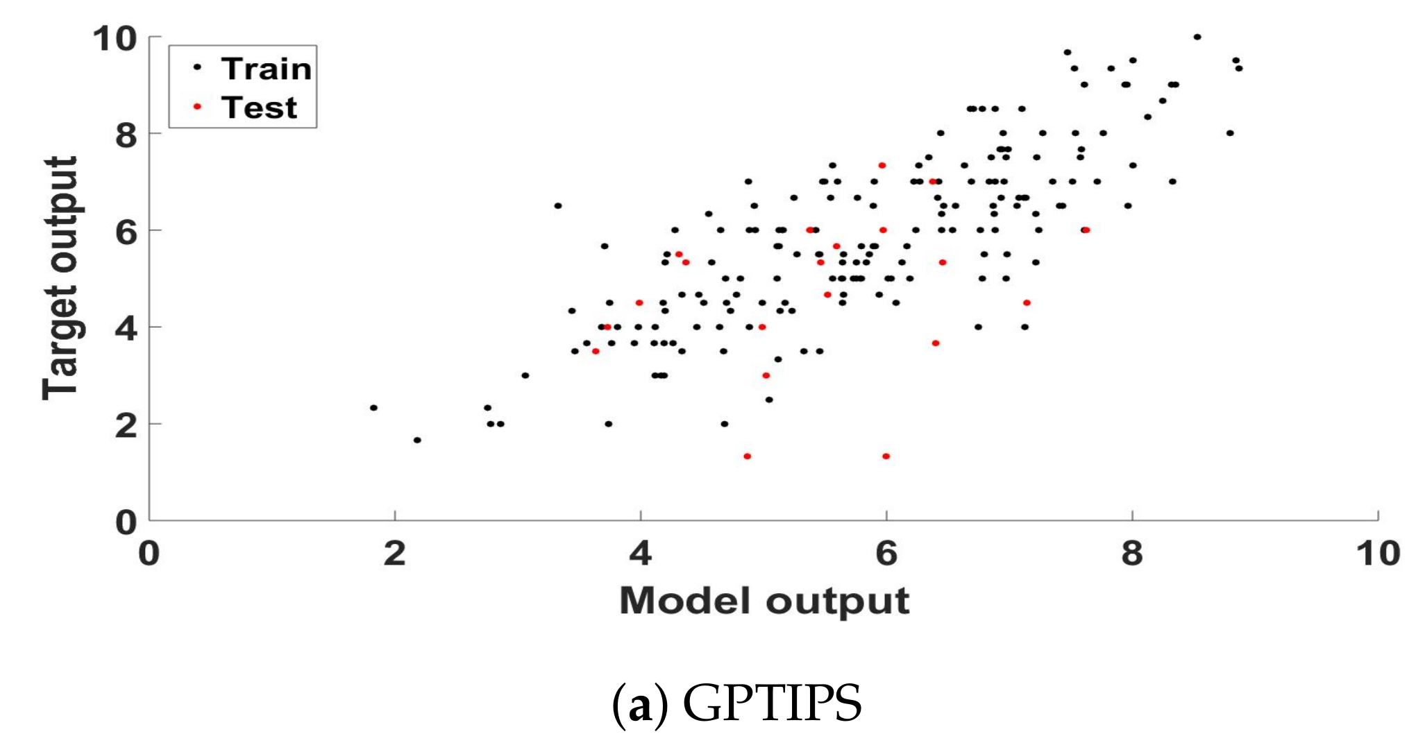
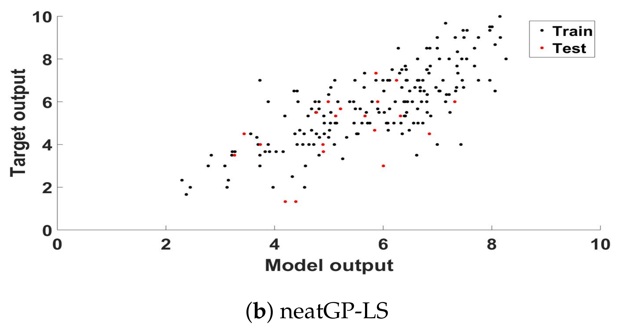
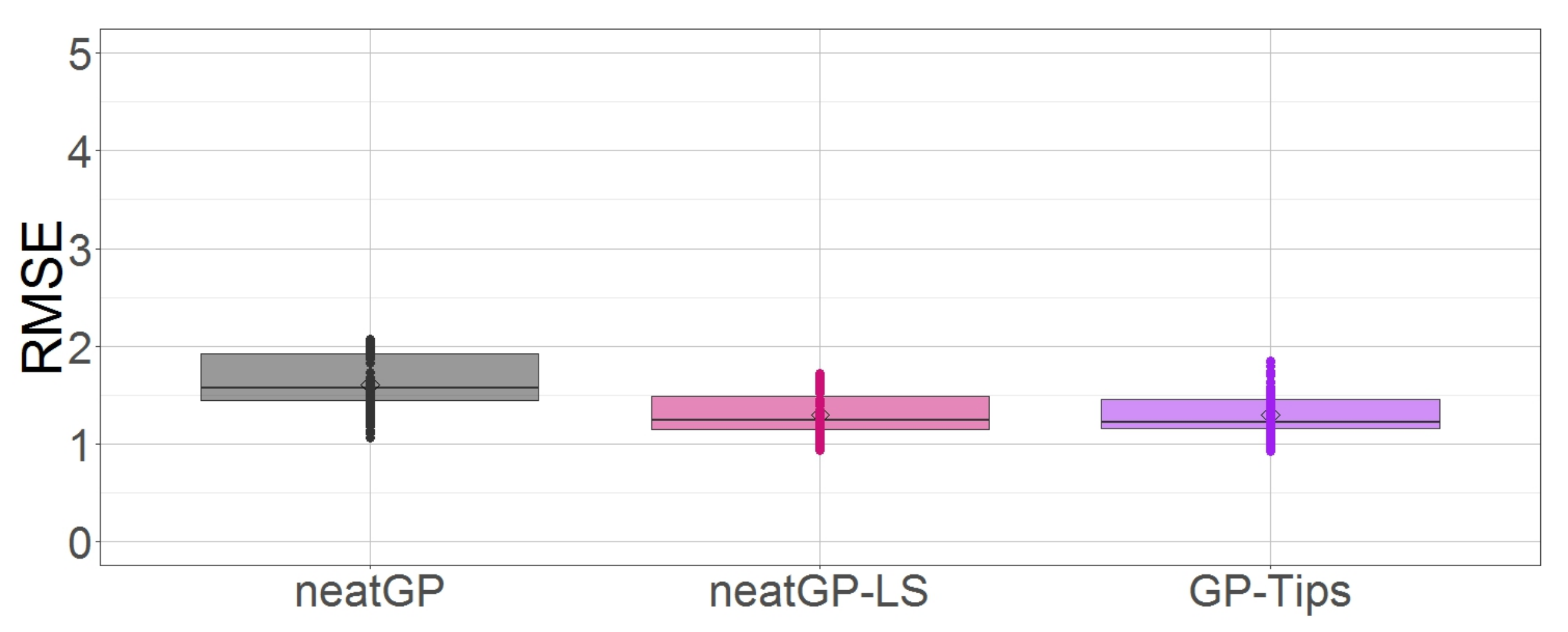
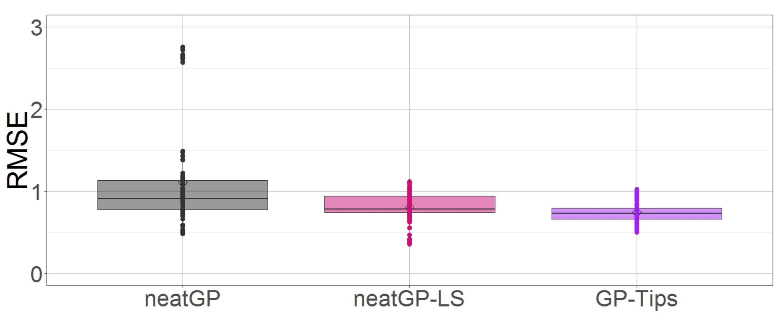
To validate the differences in the output generated by each GP strategy, we will conduct the Friedman test [22], which is a non-parametric test that helps identify if there are statistical differences in the variances of multiple treatments. For all the experiments, we will use a significance level of α = 0.05 . To present this analysis, we will make use of a Critical Difference Diagram (CDD), proposed by [23]. CDD shows in an intuitively manner how different approaches are ranked, being favored those that are located rightmost in the horizontal bar. It also shows when no statistical difference was found between a group of treatments, joining them with a thick bar.

4. Results

In this section we present the results of the execution of each GP strategy applied to the problem of finding suitable scoring functions for driving trips. A 10-fold cross validation scheme was applied in all the experiments, where the same data partitions were used by all algorithms. All of the common parameters were set to the same values, summarized in Table 2. All other parameters were set to their default values as reported in the original references.
Experiment 1: Targets in the 1–10 scale. The performance of each GP strategy is given in Table 3, Table 4 and Table 5, for GPTIPS, neatGP and neatGP-LS, respectively. The format for all comparison tables present the performance on each fold, showing the best training RMSE, the RMSE of the best solution found, the size of the best individual given in number of nodes, and the average size of the population. Summary statistics are also given, showing the minimum, maximum, mean, standard deviation, median and linear correlation coefficient of the best solutions, between the ground truth and the model output.
Figure 1 presents a scatter plot analysis of the best model found, plotting the ground truth score and the model output for each training and testing sample of that particular fold, respectively for GPTIPS (a) and neatGP-LS (b), neatGP was omitted in this comparison since it achieved the poorest results. The corresponding linear correlation coefficient, for the training and testing data, are given in the previous tables.
As a concluding remark for this subsection let us examine the distribution of the RMSE scores for all three approaches. Figure 2 shows through boxplots how GP-Tips and neatGP-LS generate models with less error than neatGP.
Experiment 2: Targets in scale 1–4. Table 6, Table 7 and Table 8 summarize the performance of GPTIPS, neatGP and neatGP-LS, respectively.
The performance over all cross-validation folds is shown in Figure 3, which is a box plot for the testing RMSE. Notice that in the scale 1–4 GPTIPS does not only presents the best performance, but also it shows the less variance.
To ilustrate a resulting evolved model of GP, Table 9 presents one of the best models found by GPTIPS from the perspective of accuracy and complexity.
Statistical analysis. To formally compare the results from each algorithm in terms of test performance (RMSE), we applied a Friedman test [22] and present this results using a Critical Difference Diagram [23], as previously stated.
Figure 4 shows a summary of the results for the 1–10 scale, showing the average rank of each method, indicating that there is no statistically significant difference between the test performance results of all GP variants.
Figure 5 presents the same analysis for the 1–4 scale. For the 1–10 scale, neatGP-LS is the top performer, although with no statistical difference. In the 1–4 scale, GPTIPS seems to have advantage, with no statistical difference with neatGP-LS but with statistical difference with neatGP.
Analysis of Features Frequency. To gain some insight about how each method is deriving the predictions of the driving score, Figure 6 plots the frequency with which each input feature appears in all of the best solutions found (a total of 10, one for each fold). Such an analysis can be useful, particularly since the models are quite compact. In the case of neatGP, where the models are larger, the frequency is notably heftier. However, probably the most useful way in which to read this plot is to consider the relative importance of each feature for each method. To associate each feature with its corresponding index variable see Figure 1. In the case of neatGP, feature x 1 is the most used by the models, followed by x 2 , and then x 6 and x 8 . On the other hand, neatGP-LS prefers x 2 , x 4 and x 6 . Additionally GPTIPS uses a smaller number of features, focusing on x 1 and x 2 . Notice that some features are practically ignored by neat-GP or GPTIPS, namely x 5 by both and x 5 , x 3 and x 4 by GPTIPS. This suggest that these features are not required and may be omitted by a real-time system that must first detect these features before scoring a driving trip.

5. Conclusions

As cities and urban areas continue to grow, the need for smart technologies that can improve safety is always of great importance. One source of great health and economic impact are traffic accidents, that can range from minor fender benders to life threatening situations. One way to help mitigate these type of accidents is to be able to automatically detect when a person is driving in an unsafe manner, to help bring about the proper corrective measures. This problem can be solved in a two-step process. First, to detect specific types of driving events that are highly correlated with safety. Second, to use the frequency of detected events to derive a safety score for a given driving trip. This paper deals with the latter, building upon previous results were the former has been solved using sensors from mobile devices [24].
This work presents an experimental evaluation of three GP algorithms to solve a difficult real-world problem. GP search is used to evolve scoring functions that take as input the frequency with which a set of driving events are detected during a trip. The goal is to have models that can accurately predict how a human observer would grade a particular trip, based on features such as average speed, distance of a trip, number of lane changes, abrupt steering, sudden stops, among others. A dataset was built, comprised by a total of 200 road trips, each one assembled as a collection of DE, and several human observers graded the trips, with the final score being an average of all scores received.
Using GP, we generated models, expressed as mathematical equations that are able to predict the scores given by humans. Three variants were tested, namely neatGP, neatGP-LS and GPTIPS. In terms of predictive accuracy no statistically significant difference was detected among the methods. However, neatGP did show the largest variance and larger number of outliers from a 10-fold cross validation evaluation. On the other hand, in terms of model size (or complexity) a clear trend was apparent, neatGP produced the largest models, while neatGP-LS and GPTIPS produced similarly concise and compact models. All three methods use a form of bloat control, neatGP and neatGP-LS use speciation and fitness sharing, while GPTIPS uses a multi-objective selection pressure. However, neatGP does not include a numerical local search optimizer, while the other two methods include one, GPTIPS uses linear regression and neatGP-LS a trust region optimizer. This indicates that in real-world problems, traditional bloat control is not sufficient. Local search methods help the evolutionary process tune smaller solutions and improve their chances of survival, curtailing bloat in favor of simpler solutions with properly tuned parameter values. A further analysis about what events are important to construct the scoring functions offers interesting insights. For GPTIPS, the distance ( x 1 ) and average velocity of the trip ( x 2 ) are important features. On its part, neatGP-LS considers the same features, but also the number of abrupt steerings ( x 8 ) and frequency of intense brakes ( x 6 ). In summary, it is clear that GP is a viable approach to solve this problem, and the evolved models are candidates for real-world testing given their accuracy and compact (efficient) form.

Acknowledgments

This project was financed by Google via a 2017 Latin American Research Award and by Proyecto Fronteras de la Ciencia CONACYT FC-2015-2/944 “Aprendizaje evolutivo a gran escala”.

Author Contributions

R.L. and L.C.G.G. designed the experiments, implemented the GPTIPS strategy and co-author the paper. O.P., G.R. and L.M. developed the dataset and implemented a Fuzzy strategy as baseline. L.T. co-author the paper and supervised the neatGP and neatGP-LS strategies. A.P. and P.J.-S. implemented the neatGP and neatGP-LS strategies and experiments

Conflicts of Interest

The authors declare no conflict of interest.

Abbreviations

The following abbreviations are used in this manuscript:
GPGenetic Programming
MLMachine Learning
SRMSymbolic Regression Model
ANNArtificial Neural Networks
SVMSupport Vector Machines
RFRandom Forest
BNBayesian Networks
FISFuzzy Inference Systems
BRRBayesian Ridge Regression
SVRSupport Vector Regression
LSLocal Search
NEATNeuroEvolution of Augmenting Topologies algorithm
Flat-OEFlat Operator Equalization
DEDriving Event
RMSERoot Mean Squared Error

References

  1. Castignani, G.; Thierry, D.; Frank, R.; Engel, T. Smartphone-Based Adaptive Driving Maneuver Detection: A Large-Scale Evaluation Study. IEEE Trans. Intell. Transp. Syst. 2017, 18, 2330–2339. [Google Scholar] [CrossRef]
  2. Handel, P.; Skog, I.; Wahlström, J.; Welch, R.; Ohlsson, J.; Ohlsson, M. Insurance telematics: Opportunities and challenges with the smartphone solution. IEEE Intell. Transp. Syst. Mag. 2014, 6, 57–70. [Google Scholar] [CrossRef]
  3. Saiprasert, C.; Thajchayapong, S.; Pholprasit, T.; Tanprasert, C. Driver Behaviour Profiling using Smartphone Sensory Data in a V2I Environment. In Proceedings of the International Conference on Connected Vehicles and Expo (ICCVE), Vienna, Austria, 3–7 November 2014. [Google Scholar]
  4. Aljaafreh, A.; Alshabatat, N.; Al-Din, N.S.M. Driving Style Recognition Using Fuzzy Logic. In Proceedings of the IEEE International Conference on Vehicular Electronics and Safety, Istanbul, Turkey, 24–27 July 2012. [Google Scholar]
  5. Eren, H.; Makinist, S.; Akin, E.; Yilmaz, A. Estimating Driving Behavior by a Smartphone. In Proceedings of the Intelligent Vehicles Symposium, Alcala de Henares, Spain, 3–7 June 2012. [Google Scholar]
  6. Al-Sultan, S.; Al-Bayatti, A.H.; Zedan, H. Context-aware driver behavior detection system in intelligent transportation systems. IEEE Trans. Veh. Technol. 2013, 62, 4264–4275. [Google Scholar] [CrossRef]
  7. López, J.R.; Gonzalez, L.C.; Gómez, M.M.; Trujillo, L.; Ramirez, G. A Genetic Programming Approach for Driving Score Calculation in the Context of Intelligent Transportation Systems. 2017; under review. [Google Scholar]
  8. Searson, D.P. Handbook of Genetic Programming Applications: Chapter 22-GPTIPS 2: An Open Source Software Platform for Symbolic Data Mining; Springer: Newcastle, UK, 2015. [Google Scholar]
  9. Trujillo, L.; Munoz, L.; Galvan-Lopez, E.; Silva, S. Neat Genetic Programming: Controlling Bloat Naturally. Inf. Sci. 2016, 333, 21–43. [Google Scholar] [CrossRef]
  10. Juárez-Smith, P.; Trujillo, L. Integrating Local Search Within neat-GP. In Proceedings of the 2016 on Genetic and Evolutionary Computation Conference Companion, Denver, CO, USA, 20–24 July 2016; pp. 993–996. [Google Scholar]
  11. Ali, N.A.; Abou-zeid, H. Driver Behavior Modeling: Developments and Future Directions. Int. J. Veh. Technol. 2016, 2016, 6952791. [Google Scholar]
  12. Dai, J.; Teng, J.; Bai, X.; Shen, Z.; Xuan, D. Mobile phone based drunk driving detection. In Proceedings of the 2010 4th International Conference on Pervasive Computing Technologies for Healthcare, Munich, Germany, 22–25 March 2010; pp. 1–8. [Google Scholar]
  13. Chaovalit, P.; Saiprasert, C.; Pholprasit, T. A method for driving event detection using SAX with resource usage exploration on smartphone platform. EURASIP J. Wirel. Commun. Netw. 2014, 2014, 135. [Google Scholar] [CrossRef]
  14. Zylius, G. Investigation of Route-Independent Aggressive and Safe Driving Features Obtained from Accelerometer Signals. IEEE Intell. Transp. Syst. Mag. 2017, 9, 103–113. [Google Scholar] [CrossRef]
  15. Davarynejad, M.; Vrancken, J. A survey of fuzzy set theory in intelligent transportation: State of the art and future trends. In Proceedings of the 2009 IEEE International Conference on Systems, Man and Cybernetics, San Antonio, TX, USA, 11–14 October 2009; pp. 3952–3958. [Google Scholar]
  16. Engelbrecht, J.; Booysen, M.; van Rooyen, G.; Bruwer, F. Performance comparison of dynamic time warping (DTW) and a maximum likelihood (ML) classifier in measuring driver behavior with smartphones. In Proceedings of the 2015 IEEE Symposium Series on Computational Intelligence, Cape Town, South Africa, 7–10 December 2015; pp. 427–433. [Google Scholar]
  17. Johnson, D.; Trivedi, M.M. Driving style recognition using a smartphone as a sensor platform. In Proceedings of the 2011 14th International IEEE Conference on Intelligent Transportation Systems (ITSC), Washington, DC, USA, 5–7 October 2011; pp. 1609–1615. [Google Scholar]
  18. Wahlström, J.; Skog, I.; Händel, P. Smartphone-Based Vehicle Telematics: A Ten-Year Anniversary. IEEE Trans. Intell. Transp. Syst. 2017, 18, 2802–2825. [Google Scholar] [CrossRef]
  19. Stanley, K.O.; Miikkulainen, R. Evolving Neural Networks through Augmenting Topologies. Evolut. Comput. 2002, 10, 99–127. [Google Scholar] [CrossRef] [PubMed]
  20. Silva, S.; Dignum, S.; Vanneschi, L. Operator Equalisation for Bloat Free Genetic Programming and a Survey of Bloat Control Methods. Genet. Program. Evolvable Mach. 2012, 13, 197–238. [Google Scholar] [CrossRef]
  21. De Rainville, F.M.; Fortin, F.A.; Gardner, M.A.; Parizeau, M.; Gagné, C. DEAP: A Python Framework for Evolutionary Algorithms. In Proceedings of the 14th Annual Conference Companion on Genetic and Evolutionary Computation GECCO’12, Philadelphia, PA, USA, 7–11 July 2012; pp. 85–92. [Google Scholar]
  22. Conover, W.J. Practical Nonparametric Statistics, 3rd ed.; John Wiley: New York, NY, USA, 1999. [Google Scholar]
  23. Demšar, J. Statistical Comparisons of Classifiers over Multiple Data Sets. J. Mach. Learn. Res. 2006, 7, 1–30. [Google Scholar]
  24. Carlos, M.R.; Gonzalez, L.C.; Ramirez, G. Unsupervised Feature Extraction for the Classification of Risky Driving Maneuvers. 2017; under review. [Google Scholar]
Figure 1. Scatter plot of the ground truth scores and the model outputs for the training and testing partitions of the best solution found computed for the dataset with a 1–10 scale.
Mca 23 00019 g001aMca 23 00019 g001b
Figure 2. Box plot comparison of all methods based on testing fitness on the dataset with a 1–10 scale.
Mca 23 00019 g002
Figure 3. Box plot comparison of all methods based on testing fitness on the dataset with a 1–4 scale.
Mca 23 00019 g003
Figure 4. Critical Difference Diagram (CDD) of the Friedman test for the 1–10 scale problem.
Mca 23 00019 g004
Figure 5. CDD of the Friedman test for the 1–4 scale problem.
Mca 23 00019 g005
Figure 6. Frequency of appearance of each DE (feature variables x 1 to x 8 ) in the best solutions found by each method on the dataset.
Mca 23 00019 g006
Table 1. A sample of the survey used to evaluate each driving event as safe or unsafe, based on the frequency of each DE.
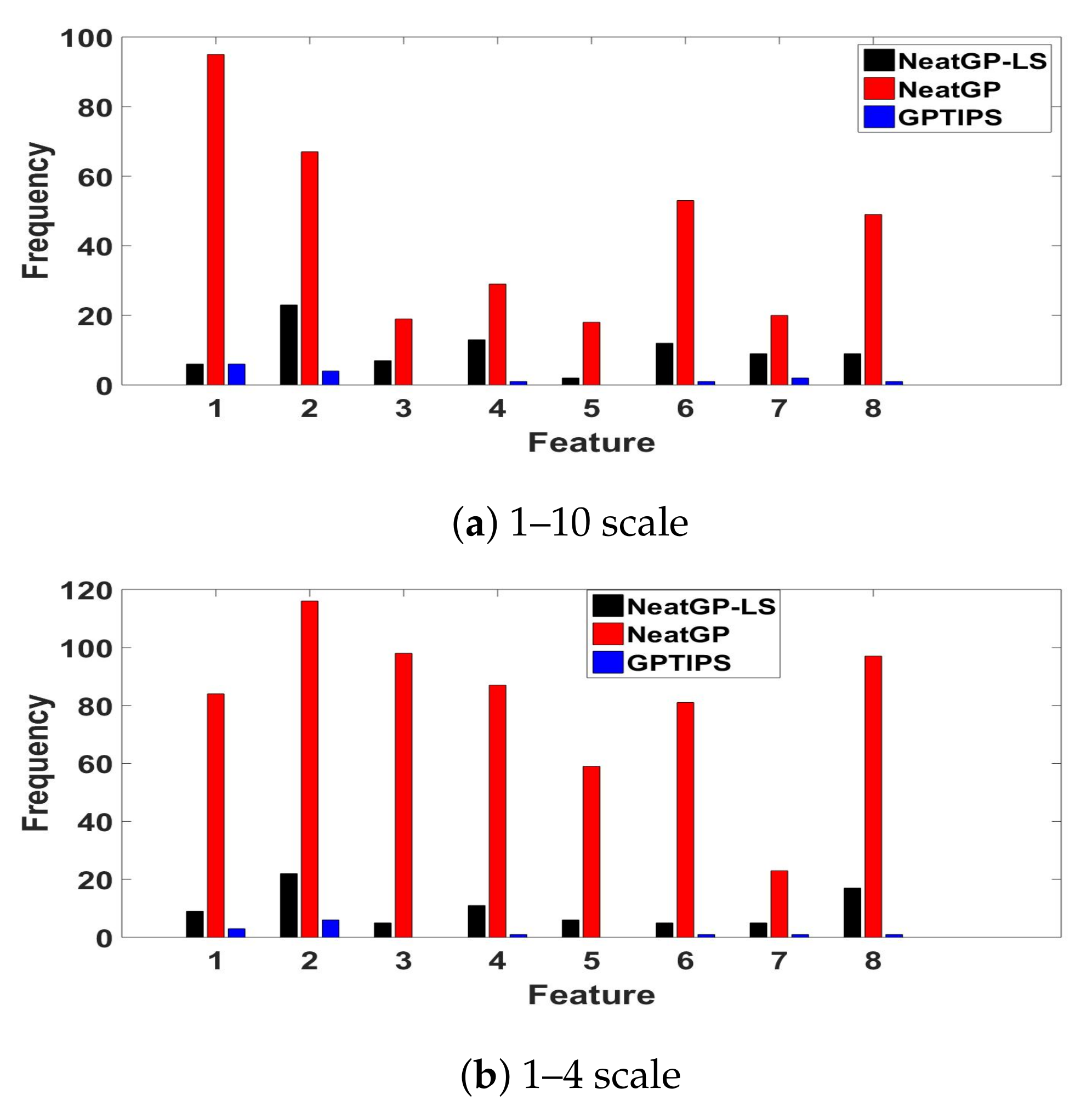
Driving Event (id Number in the Feature Vector)Value (Frequency)Score for the Travel
Distance ( x 1 )7
Avg. Velocity ( x 2 )6
# of acceleration events ( x 3 )5
# of sudden starts ( x 4 )38
# of abrupt lane changes ( x 5 )2
# of intense brakes ( x 6 )7
# of sudden stops ( x 7 )0
# of abrupt steerings ( x 8 )1
Table 2. Parameters for GPTIPS, neatGP and neatGP-LS.
ParameterValueUnits
Population size100items
Max. # of generations100items
Input variables8items
Range of Constants[−10, 10]items
Training instances180road trips
Testing instances20road trips
Crossover probability85percentage (%)
Mutation probability15percentage (%)
Function set × , , + , ÷ , x , functions
tanh , exp , log , x 3 ,
M U L T 3 , A D D 3 ,
n e g e x p , n e g , | x |
Table 3. Root Mean Squared Error (RMSE) for the 10-fold cross validation performance of GPTIPS on the 1–10 scale dataset.
GPTIPS
FoldBest TrainBest TestSize Best IndAvg. Pop. Size
11.12191.22112221.1200
21.11681.21882522.6067
31.13291.04822220.0633
41.09781.45092623.6000
51.14791.00342522.7067
61.12961.15462424.3533
71.13671.18572423.2800
81.06501.78542523.0167
91.13561.31302322.2233
101.05951.55602221.1667
Minimum1.05951.00342220.0633
Maximum1.14791.78542624.3533
mean1.11441.293723.800022.4137
SD0.03060.24081.47571.2994
median1.12571.219924.000022.6567
Correlation Coefficient0.80300.2868
Table 4. RMSE for the 10-fold cross validation performance of neatGP on the 1–10 scale dataset.
neatGP
FoldBest TrainBest TestSize Best IndAvg. Pop. Size
11.20931.57954639.1850
21.25841.14886445.9650
31.82911.9927183124.3400
41.39281.3015132100.0250
51.30641.51714427.9500
61.29691.97536144.3100
70.85051.5701625211.0900
81.22611.62906954.6200
91.24961.92546647.0100
101.25461.43814429.5650
Minimum0.85051.14884427.9500
Maximum1.82911.9927625211.0900
mean1.28741.6077133.400072.4060
SD0.23780.2845178.420457.7911
median1.25651.574865.000046.4875
Correlation Coefficient0.64320.6337
Table 5. RMSE for the 10-fold cross validation performance of neatGP-LS on the 1–10 scale dataset.
neatGP-LS
FoldBest TrainBest TestSize Best IndAvg. Pop. Size
11.16901.69123011.5900
21.21951.16234011.9700
31.16221.26262216.0000
41.21881.05133118.8400
51.17561.56572916.1750
61.18131.03103620.1050
71.37581.373913.4200
81.18221.14561818.5950
91.13261.48993113.2200
101.19171.22023516.5700
Minimum1.13261.031013.4200
Maximum1.37581.69124020.1050
mean1.20091.299427.300014.6485
SD0.06660.223611.25514.8923
median1.18181.241430.500016.0875
Correlation Coefficient0.77350.5012
Table 6. RMSE for the 10-fold cross validation performance of GPTIPS on the 1–4 scale dataset.
GPTIPS
FoldBest TrainBest TestSize Best IndAvg. Pop. Size
10.64450.73472222.0300
20.65670.65911817.7833
30.64740.74082121.8767
40.62150.95302323.9733
50.66040.68332924.4567
60.64910.79312018.0233
70.66300.59132220.8233
80.65240.64002922.3667
90.64020.72412119.9933
100.61760.92862321.7733
Minimum0.61760.59131817.7833
Maximum0.66300.95302924.4567
mean0.64530.744822.800021.3100
SD0.01530.11823.58392.2205
median0.64820.729422.000021.8250
Correlation Coefficient0.75050.6219
Table 7. RMSE for the 10-fold cross validation performance of neatGP on the 1–4 scale dataset.
neatGP
FoldBest TrainBest TestSize Best IndAvg. Pop. Size
10.60702.6656234174.0650
20.57700.9034276169.5550
30.80560.8421464266.4800
40.65131.1010176118.1200
50.47050.5493236151.3600
60.50381.1317245160.8900
70.67480.7746159110.3400
80.70930.74635542.1850
90.52840.9176205146.1850
100.54911.426013965.5550
Minimum0.47050.54935542.1850
Maximum0.80562.6656464266.4800
mean0.60771.1058218.9000140.4735
SD0.10340.5991107.188862.4507
median0.59200.9105219.5000148.7725
Correlation Coefficient0.88050.5857
Table 8. RMSE for the 10-fold cross validation performance of neatGP-LS on the 1–4 scale dataset.
neatGP-LS
FoldBest TrainBest TestSize Best IndAvg. Pop. Size
10.63870.98523018.9650
20.72400.74772916.7000
30.66750.78542814.3150
40.62910.93843720.5550
50.63210.78102116.1550
60.66110.78514124.1900
70.72170.45192919.7950
80.63370.63873419.5900
90.66220.94082915.8750
100.63231.01981714.0850
Minimum0.62910.45191714.0850
Maximum0.72401.01984124.1900
mean0.66030.807429.500018.0225
SD0.03590.17386.99603.1629
median0.64990.785229.000017.8325
Correlation Coefficient0.75980.3352
Table 9. ith Best model in the Pareto front, from the stand point of accuracy and complexity (1–4 scale) (GPTIPS).
RMSE TestingComplexity (# of Nodes)Model
0.91937
y = 0.4486 e 1.0 x 1 x 1 1.0 x 1 x 2 9.9 x 2 0.05036 x 8 0.02518 tanh tanh x 4 tanh tanh x 4 1.0 x 1 x 2 9.9 0.2356 x 2 + 3.443

