A Simple Spectral Observer

Abstract

The principal aim of a spectral observer is twofold: the reconstruction of a signal of time via state estimation and the decomposition of such a signal into the frequencies that make it up. A spectral observer can be catalogued as an online algorithm for time-frequency analysis because is a method that can compute on the fly the Fourier Transform (FT) of a signal, without having the entire signal available from the start. In this regard, this paper presents a novel spectral observer with an adjustable constant gain for reconstructing a given signal by means of the recursive identification of the coefficients of a Fourier series. The reconstruction or estimation of a signal in the context of this work means to find the coefficients of a linear combination of sines a cosines that fits a signal such that it can be reproduced. The design procedure of the spectral observer is presented along with the following applications: (1) the reconstruction of a simple periodical signal, (2) the approximation of both a square and a triangular signal, (3) the edge detection in signals by using the Fourier coefficients, (4) the fitting of the historical Bitcoin market data from 1 December 2014 to 8 January 2018 and (5) the estimation of a input force acting upon a Duffing oscillator. To round out this paper, we present a detailed discussion about the results of the applications as well as a comparative analysis of the proposed spectral observer vis-à-vis the Short Time Fourier Transform (STFT), which is a well-known method for time-frequency analysis.

1. Introduction

The term spectral observer was proposed by Hostetter in his pioneering work [1] to name the algorithm that permits the recursive calculation of the Fourier Transform (FT) of a band-limited signal via state estimation. Since the presentation of such a work, several designs of spectral observers with improved features have been proposed either to deal with noise [2], disturbances, lack of data [3] or to estimate other parameters such as frequency [4]. The main goals of a spectral observer are both the estimation of a given signal and the transformation of such a signal to the frequency domain by means of the recursive identification of the coefficients of a Fourier series [5]. The estimation of a signal in the context of this work means to find the coefficients of a linear combination of functions—sines a cosines functions in our case—that approximates a signal of interest such that it can be reconstructed [6]. Spectral observers are useful in a wide number of applications, e.g., for determining the source of harmonic pollution in power systems [7], for the simulation of the sea surface [8], for fault diagnosis in motors [9,10] or in vibrating structures, such as aerospace and mechanical structures, marine structures, buildings, bridges and offshore platforms.

A spectral observer can be catalogued as an online algorithm to compute the Fourier Transform (FT) during a time window which slides along the signal, i.e., an algorithm to compute the Short Time Fourier Transform (STFT). Therefore, a spectral observer can be used for the time-frequency analysis of frequency variant signals.

The observer that we propose in this contribution is designed from a dynamical system which is constructed from the N derivatives of a n-th order Fourier series.

To perform the estimation, the observer solely requires: (1) The measurement of the signal to be approximated, $s\left(t\right)$, which actually is used to compute the observation error $e\left(t\right)=s\left(t\right)-\widehat{y}\left(t\right)$, where $\widehat{y}\left(t\right)$ is the observer output, (2) A frequency step $\omega =2\pi /T$, where T is a predefined period. The estimation provided by the observer are both the reconstruction of the original signal and the Fourier coefficients to compute the signal frequency components.

This paper is organized as follows: Section 2 presents the core of the proposed method which is the formulation of the spectral observer from the Fourier series. Section 3 presents some examples with test results of the proposed method utilized in different applications. In Section 4 the main results are discussed. Finally, in Section 5 some concluding thoughts are given.

2. The Proposed Method

To construct the proposed observer, we formulate a dynamical synthetic system in state space representation by considering, firstly, that a given signal expressed as $s\left(t\right)$ can be approximated by a Fourier series, and secondly, that the Fourier series is the first state of the system and the rest of the states are the N first-order derivatives of the Fourier series expressed by Equation (1), where n is the series order.

$$y\left(t\right)=\frac{a_0}{2}+\sum _{k=1}^n\left[a_k\cos \left(k\omega t\right)+b_k\sin \left(k\omega t\right)\right],$$

(1)

where $a_0,a_1,b_1,\dots ,a_n,b_n$ are the Fourier coefficients and $\omega$ is the fundamental angular frequency of the signal to be estimated.

In this work, we assume that the signal $s\left(t\right)$ to be approximated has not a constant component (offset) or that this offset is removed by an online algorithm prior to be processed by the spectral observer. For this reason, we remove the term $a_0$ from Equation (1) such that the series for approximating the time function $s\left(t\right)$ can be expressed as follows

$$y\left(t\right)=\sum _{k=1}^n\left[a_k\cos \left(k\omega t\right)+b_k\sin \left(k\omega t\right)\right].$$

(2)

If the order of the Fourier series is $n=1$, we need to formulate a dynamical system with $N=2$ states, each one to recover each coefficient ($a_1$ and $b_1$). Thus, the two first states are the Fourier series and its first derivative.

$$\begin{array}{c}\hfill {\nu }_1\left(t\right)=y\left(t\right)=a_1\cos \left(\omega t\right)+b_1\sin \left(\omega t\right),{\nu }_2\left(t\right)=\dot{y}\left(t\right)=-\omega a_1\sin \left(\omega t\right)+\omega b_1\cos \left(\omega t\right).\end{array}$$

(3)

where ${\nu }_i$ are the states of the synthetic system. Consequently, the dynamical system that results from the change of coordinates, gives:

$$\begin{array}{c}\hfill {\dot{\nu }}_1\left(t\right)={\nu }_2\left(t\right),{\dot{\nu }}_2\left(t\right)=-{\omega }^2{\nu }_1\left(t\right),\end{array}$$

(4)

which basically is the dynamical model of a harmonic oscillator. Now, what happens if the order of the Fourier series increases? If the order increases to $n=2$, then $N=4$, since we need to recover four coefficients.

$$\begin{array}{ccc}\hfill {\nu }_1\left(t\right)& =& y\left(t\right)=a_1\cos \left(\omega t\right)+b_1\sin \left(\omega t\right)+a_2\cos \left(2\omega t\right)+b_2\sin \left(2\omega t\right),\hfill \\ \hfill {\nu }_2\left(t\right)& =& \dot{y}\left(t\right)=-\omega a_1\sin \left(\omega t\right)+\omega b_1\cos \left(\omega t\right)-2\omega a_2\sin \left(2\omega t\right)+2\omega b_2\cos \left(2\omega t\right),\hfill \\ \hfill {\nu }_3\left(t\right)& =& \ddot{y}\left(t\right)=-{\omega }^2{a}_1\cos \left(\omega t\right)-{\omega }^2{b}_1\sin \left(\omega t\right)-4{\omega }^2{a}_2\cos \left(2\omega t\right)-4{\omega }^2{b}_2\sin \left(2\omega t\right),\hfill \\ \hfill {\nu }_4\left(t\right)& =& y^{\left(3\right)}\left(t\right)={\omega }^3{a}_1\sin \left(\omega t\right)-{\omega }^3{b}_1\cos \left(\omega t\right)+8{\omega }^3{a}_2\sin \left(2\omega t\right)-8{\omega }^3{b}_2\cos \left(2\omega t\right),\hfill \\ \hfill {\dot{\nu }}_4\left(t\right)& =& y^{\left(4\right)}\left(t\right)={\omega }^4{a}_1\cos \left(\omega t\right)+{\omega }^4{b}_1\sin \left(\omega t\right)+16{\omega }^4{a}_2\cos \left(2\omega t\right)+16{\omega }^4{b}_2\sin \left(2\omega t\right).\hfill \end{array}$$

(5)

The dynamical system is then formulated as in Equation (5) which, after some algebraic manipulations, it becomes

$$\begin{array}{c}\hfill {\dot{\nu }}_1\left(t\right)={\nu }_2\left(t\right);{\dot{\nu }}_2\left(t\right)={\nu }_3\left(t\right),{\dot{\nu }}_3\left(t\right)={\nu }_4\left(t\right),{\dot{\nu }}_4\left(t\right)=-4{\omega }^4{\nu }_1\left(t\right)-5{\omega }^2{\nu }_3\left(t\right),\end{array}$$

(6)

in $\nu$-coordinates.

By generalizing Equation (5) for order n, we obtain the following dynamical system:

$$\begin{array}{cc}\hfill {\dot{\nu }}_1\left(t\right)& ={\nu }_2\left(t\right),\hfill \\ \hfill {\dot{\nu }}_2\left(t\right)& ={\nu }_3\left(t\right),\hfill \\ \hfill ⋮& =⋮,\hfill \\ \hfill {\dot{\nu }}_N\left(t\right)& ={(-1)}^{n\left(\mathrm{mod}2\right)}{\omega }^{2n}\left[\begin{array}{cccc}1& 2^{2n}& \cdots & n^{2n}\end{array}\right]A_k^{-1}{A}_{\omega }^{-1}\nu \left(t\right),\hfill \end{array}$$

(7)

where $N=2n$, $A_{\omega }$ and $A_k$ are expressed by Equations (8) and (9), respectively.

$$A_{\omega }\doteq \left[\begin{array}{cccccccc}1& 0& 0& 0& \cdots & 0& \cdots & 0\\ 0& \omega & 0& 0& \cdots & 0& \cdots & 0\\ 0& 0& -{\omega }^2& 0& \cdots & 0& \cdots & 0\\ 0& 0& 0& -{\omega }^3& \cdots & 0& \cdots & 0\\ ⋮& ⋮& ⋮& ⋮& \ddots & ⋮& \ddots & ⋮\\ 0& 0& 0& 0& \cdots & {(-1)}^{\left(m\right(\mathrm{mod}4)-m(\mathrm{mod}2\left)\right)/2}{\omega }^m& \cdots & 0\\ ⋮& ⋮& ⋮& ⋮& \ddots & ⋮& \ddots & ⋮\\ 0& 0& 0& 0& \cdots & 0& \cdots & {(-1)}^{\left(2n\right(\mathrm{mod}4)-2)/2}{\omega }^{2n-1}\end{array}\right],$$

(8)

$$A_k\doteq \left[\begin{array}{ccccccc}1& 0& 1& 0& \cdots & 1& 0\\ 0& 1& 0& 2& \cdots & 0& n\\ 1& 0& 4& 0& \cdots & n^2& 0\\ 0& 1& 0& 8& \cdots & 0& n^3\\ ⋮& ⋮& ⋮& ⋮& \ddots & ⋮& ⋮\\ 1& 0& 2^{2n-2}& 0& \cdots & n^{2n-2}& 0\\ 0& 1& 0& 2^{2n-1}& \cdots & 0& n^{2n-1}\end{array}\right].$$

(9)

Before presenting the state observer for system (7), it is necessary to analyze its observability conditions. A dynamical system is said to be observable if it is possible to determine its initial state by knowledge of the input and output over a finite time interval. In this way, a state observer or state estimator is a system that estimates the internal states of a system from the measurement of its inputs and outputs. To verify is a linear systems is observable, the observability rank condition can be used, which is defined in the net lines.

Observability rank condition. A system

$$\begin{array}{ccc}\hfill \dot{\nu }\left(t\right)& =& A\left(t\right)\nu \left(t\right)\hfill \\ \hfill y\left(t\right)& =& C\nu \left(t\right)\hfill \end{array}$$

(10)

is said to satisfy the observability rank condition if $\forall \nu \left(t\right),\mathrm{rank}\left(O\left(\nu \right(t\left)\right)\right)=N,$ where N is the state dimension of (10) and $O\left(\nu \right(t\left)\right)$ is the observability matrix defined as

$$O\left(\nu \left(t\right)\right)={(CCAC{A}^2\dots C{A}^{(N-1)})}^T.$$

(11)

Thus, according to the definition, the observability matrix for system (7), which in fact can be set as system (10) with

$$A=\left[\begin{array}{ccccc}0& 1& \dots & 0& 0\\ 0& 0& 1& \dots & 0\\ & & & \ddots & ⋮\\ ⋮& & & & 1\\ {\gamma }_1\left(\omega \right)& & \dots & & {\gamma }_n\left(\omega \right)\end{array}\right],$$

(12)

and $C=[1,0,\dots ,0]$, has full rank. Therefore, since system (7) is observable, a spectral observer can be designed as follows:

$$\dot{\widehat{\nu }}\left(t\right)=A\widehat{\nu }\left(t\right)+K(y\left(t\right)-C\widehat{\nu }\left(t\right)),\widehat{y}\left(t\right)=C\widehat{\nu }={\widehat{\nu }}_1.$$

(13)

where “$\widehat{}$” means estimation, $\widehat{y}\left(t\right)$ is the estimated signals and A is given by (12), with constant coefficients expressed by ${\gamma }_i\left(\omega \right)$. The gain of the state observer K, involved in the correction term of Equation (13), can be calculated as $K=S^{-1}{C}^T$, where S is the unique solution of the following algebraic Lyapunov equation:

$$-\lambda S-A^{T}S-SA+C^{T}C=0$$

(14)

and $\lambda$ is a parameter that can be used to tune the convergence rate of the observer. A numerical solution for solving Equation (14) for a particular but common case is provided in [11].

The Fourier coefficients can be recovered from the new coordinates by the relation ${\widehat{c}}_k=\Omega \left(t\right)\widehat{\nu }\left(t\right)$, where ${\widehat{c}}_k={[{\widehat{a}}_1{\widehat{b}}_1\dots {\widehat{a}}_n{\widehat{b}}_n]}^T$ and

$$\begin{array}{c}\hfill \Omega \left(t\right)=\left(\begin{array}{ccccccc}▴\left(\omega t\right)& ▾\left(\omega t\right)& ▴\left(2\omega t\right)& ▾\left(2\omega t\right)& \dots & ▴\left(n\omega t\right)& ▾\left(n\omega t\right)\\ -\omega ▾\left(\omega t\right)& \omega ▴\left(\omega t\right)& -2\omega ▾\left(2\omega t\right)& 2\omega ▴\left(2\omega t\right)& \dots & -n\omega ▾\left(n\omega t\right)& n\omega ▴\left(n\omega t\right)\\ -{\omega }^2▴\left(\omega t\right)& -{\omega }^2▾\left(\omega t\right)& -4{\omega }^2▴\left(2\omega t\right)& -4{\omega }^2▾\left(2\omega t\right)& \dots & -n^2\omega ▴\left(n\omega t\right)& -n^2\omega ▾\left(n\omega t\right)\\ ⋮& & & & & & ⋮\\ {\omega }^{\Gamma }▾\left(\omega t\right)& -{\omega }^{\Gamma }▴\left(\omega t\right)& 2^{\Gamma }{\omega }^{\Gamma }▾\left(2\omega t\right)& -2^{\Gamma }{\omega }^{\Gamma }▴\left(2\omega t\right)& \dots & n^{\Gamma }{\omega }^{\Gamma }▾\left(n\omega t\right)& -n^{\Gamma }{\omega }^{\Gamma }▴\left(n\omega t\right)\end{array}\right)\end{array}$$

Notice that $▴\triangleq \cos$, $▾\triangleq \sin$ and $\Gamma \triangleq n-1$. Check Figure 1 to see a schema of the estimation.

Before presenting some possible applications of the spectral observer it is important to highlight an important point. Notice that matrix A of the spectral observer depends on the fundamental frequency $\omega$. This means that this variable must be known. In case we want to approximate a periodic signal with a known fundamental frequency, we just need to use it in matrix A. In case we want to fit a periodic signal with unknown fundamental frequency or a non-periodic signal, we must assume, as in the Fourier Transform deduction from the Fourier series, that the period of the signal tends to infinity, which means that the fundamental frequency tends to zero. As a consequence of this assumption, $\omega$ should be chosen sufficiently small or according to the desired precision in the recovery of the frequency components. In other words $\omega$ is the frequency step that determines the resolution of the discretized frequency domain, such that we have to choose $\omega$ thinking how close we want the frequency components.

3. Application Examples

This section presents five examples of possible applications of the spectral observer, which were conceived such that the reader can be able to reproduce them.

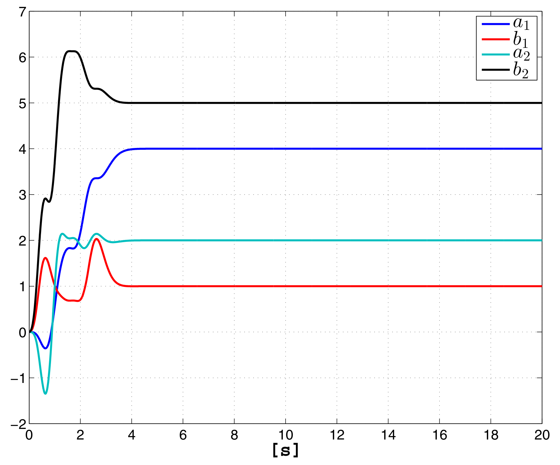
3.1. Example 1: A Simple Example

Let be the signal $s\left(t\right)=4\cos \left(t\right)+\sin \left(t\right)+2\cos \left(2t\right)+5\sin \left(2t\right)$. It is obvious that the series order to reproduce the signal is $n=2$, then the order of system (7) for the conception of the observer should be $N=4$. Figure 2 shows the estimation of the coefficients that was performed by the observer with a gain $\lambda =8$, which actually was initialized with $\widehat{\nu }\left(0\right)=0$. The step time to perform the estimation in Simulink was $\Delta t=0.005$ [s] and the used solver was ODE3.

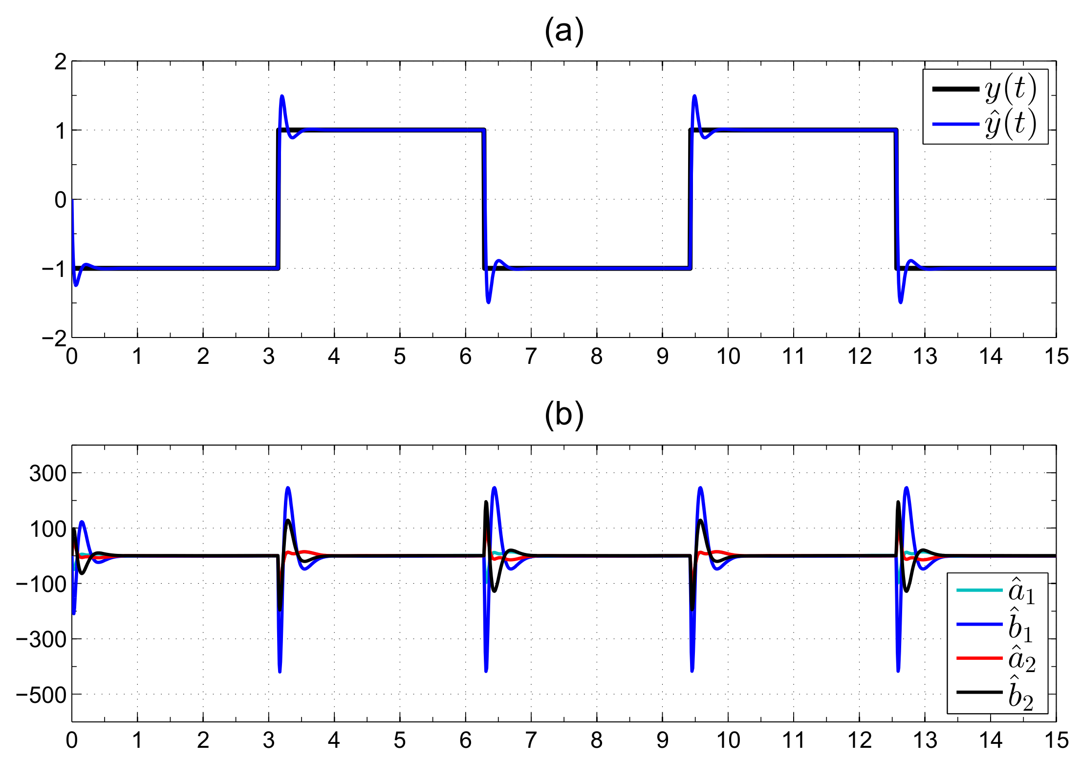
3.2. Example 2: Reconstruction of Basic Signals

This example aims to show the estimation of the coefficients for basic signals such as square and sawtooth waves. The first signal to be estimated is a square wave with angular frequency $\omega =1$ [rad/s]. The observer was tuned with $\lambda =15$. The order of the series was set $n=2$, i.e., $N=4$. The frequency step was set $\omega =5$ [rad/s]. The step time to perform the estimation in Simulink was set $\Delta t=0.01$ [s] and the used solver was ODE3. Figure 3 shows the signal reconstruction performed by the spectral observer and the estimated coefficients. Firstly, notice that the coefficients do not converge towards a constant value; the reason for this is the number of coefficients used to approximate the signal, which is not enough to represent each harmonic that composes it. Even though the coefficients are not constant, the signal is estimated. Notice too that all the coefficients change abruptly at each discontinuity. This feature can be used for edge detection as will be seen in the next example.

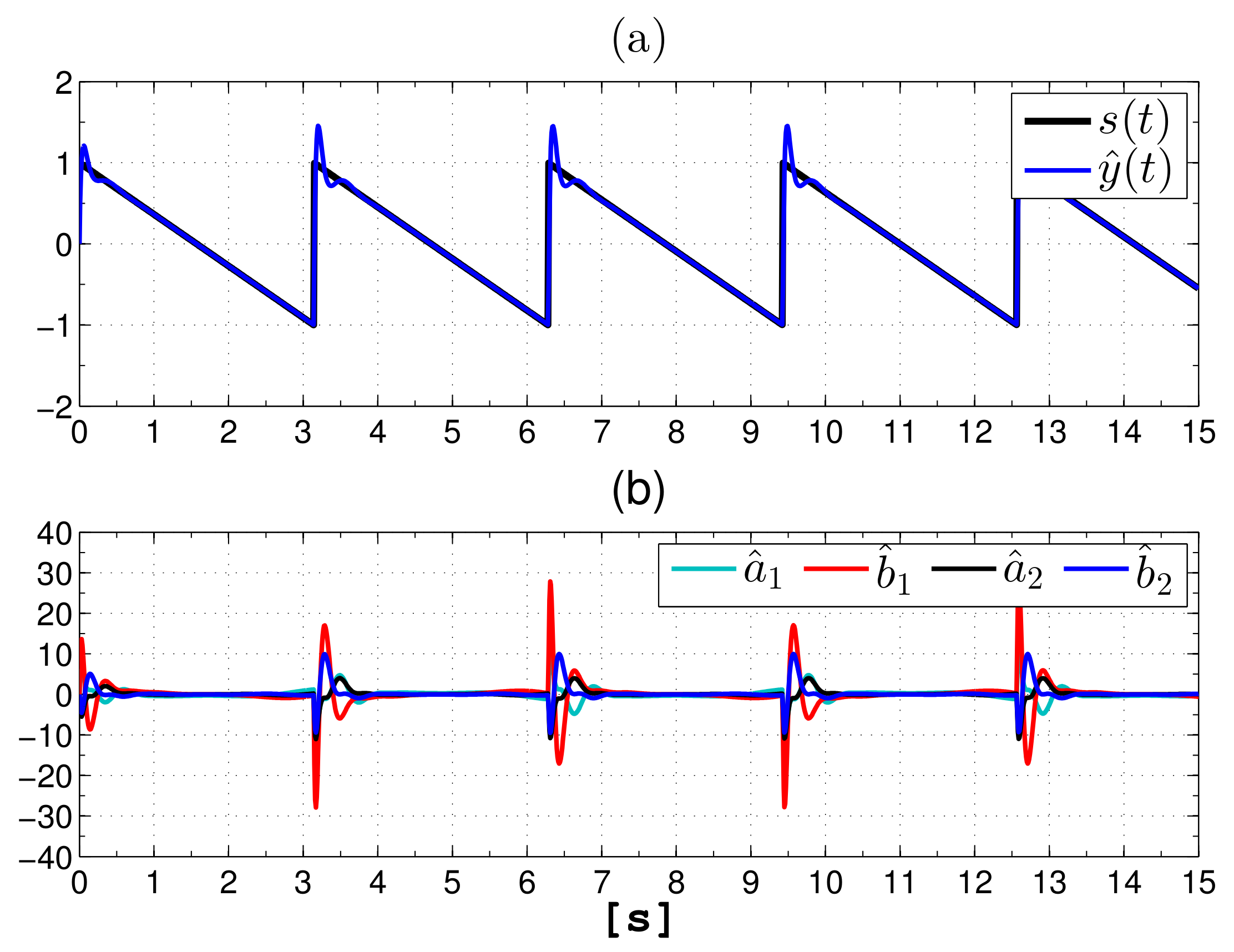
Both the observer and conditions that were used to reconstruct the square wave were used to reconstruct the sawtooth signal shown in Figure 4. Notice that the convergence time is less than one second and the coefficients become greater at the discontinuities.

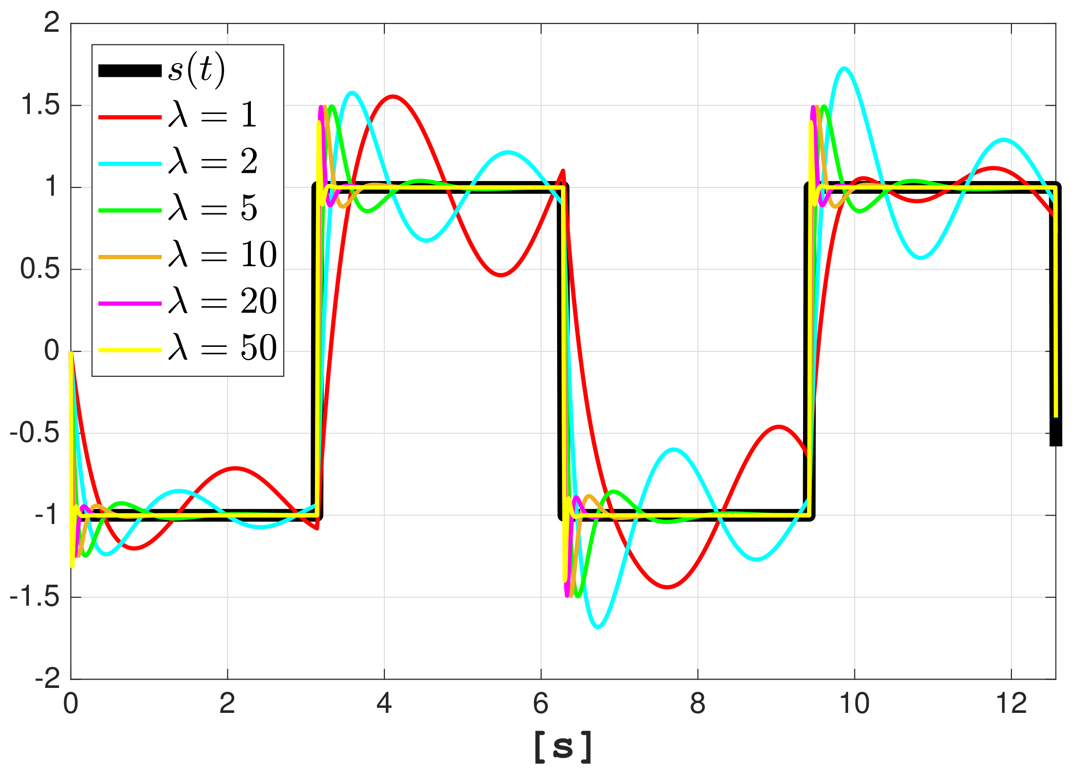
To end this example, we made several simulations to show how the parameter $\lambda$ determines the convergence period of the estimation. Figure 5 shows the estimation of the square signal with different values of $\lambda$. Notice that the bigger its value, the faster is the convergence.

3.3. Example 3: Edge Detection by Using the Fourier Coefficients

Edge detection and the detection of discontinuities are important in many fields. In image processing, for example, one often needs to determine the boundaries of the items of which a picture is composed, [12] or in applications that utilize time-domain reflectometry (TDR), which is a measurement technique used to determine the characteristics of transmission lines by observing reflected waveforms. TDR analysis begins with the propagation of a step or impulse of energy into a system and the subsequent observation of the energy reflected by the system. By analyzing the magnitude, duration and shape of the reflected waveform, the nature of the transmission system can be determined. TDR is a common method used to localize faults in transmission lines—such a leaks in pipelines or faults with small impedance in wires—because faults in transmission lines cause discontinuities in the reflected waveforms. For this reason, methodologies to detect discontinuities are required in order to localize the nature and position of the faults.

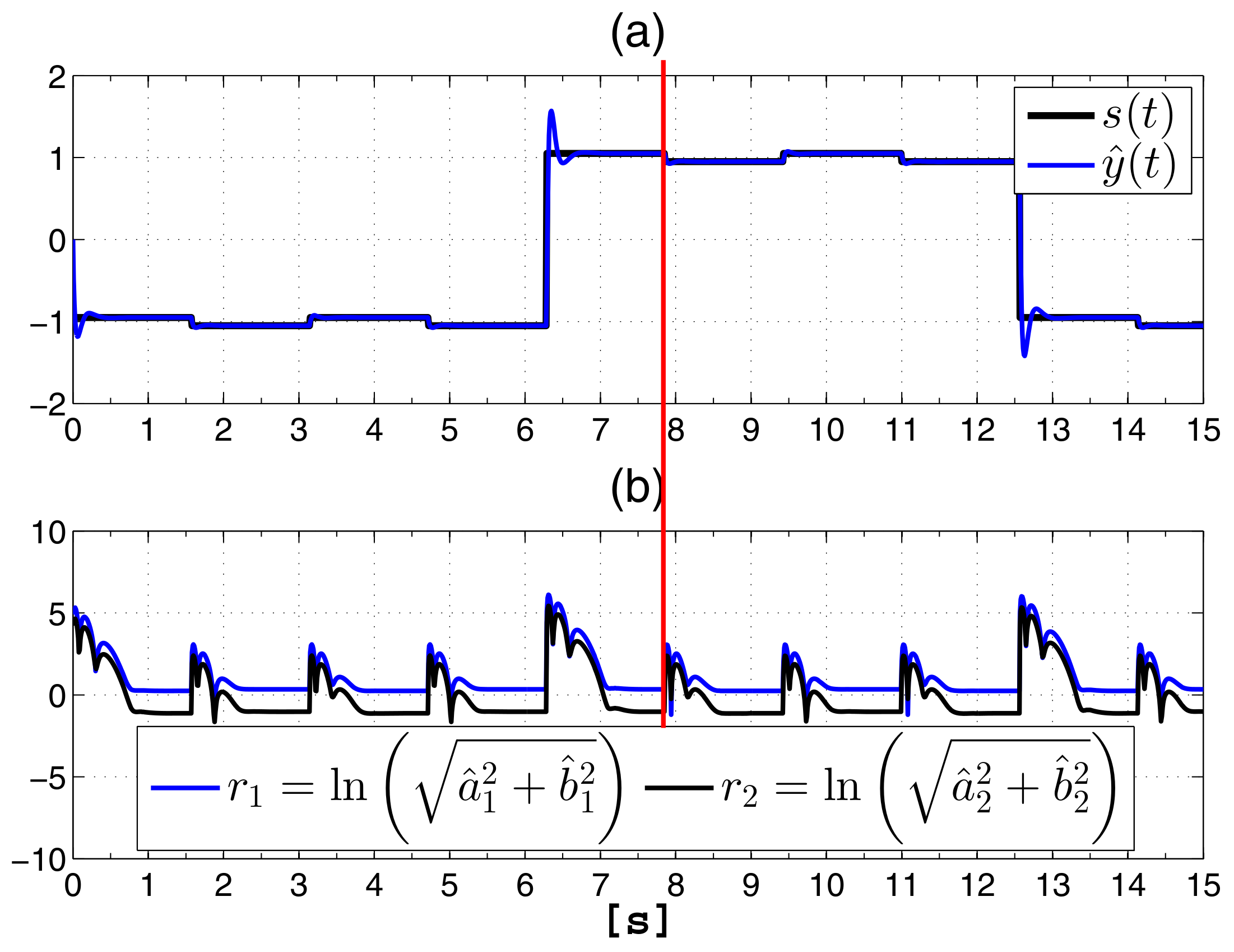
In order to shows how the spectral observer (13) can be used to detect discontinuities in a function, we present the following example: Let us consider $s\left(t\right)=\mathrm{sign}\left(\sin \left(0.5t\right)\right)-0.05\mathrm{sign}\left(\sin \left(2t\right)\right)$, which is plot in Figure 6a. The aim of this test is to detect the discontinuities in the principal signal with period $T=2$ [s]. To identify the discontinuities, the coefficients provided by the spectral observer are used to calculate the following indicator function:

$$r_k=\ln \left(\sqrt{{\widehat{a}}_k^2+{\widehat{b}}_k^2}\right)$$

(15)

The observer to perform the estimation was tuned with $\lambda =15$. The order of the series was set $n=2$, i.e., $N=4$. The frequency step was set $\omega =1$ [rad/s]. The step time to perform the estimation in Simulink was set $\Delta t=0.01$ [s] and the used solver was ODE3.

Figure 6a shows $s\left(t\right)$ and its reconstruction $\widehat{y}\left(t\right)$. Figure 6b shows the index $r_1\left(t\right)$ and $r_2\left(t\right)$ that becomes greater at the discontinuities indicating where they are.

3.4. Example 4: Fitting Complex Signal: The Bitcoin Price

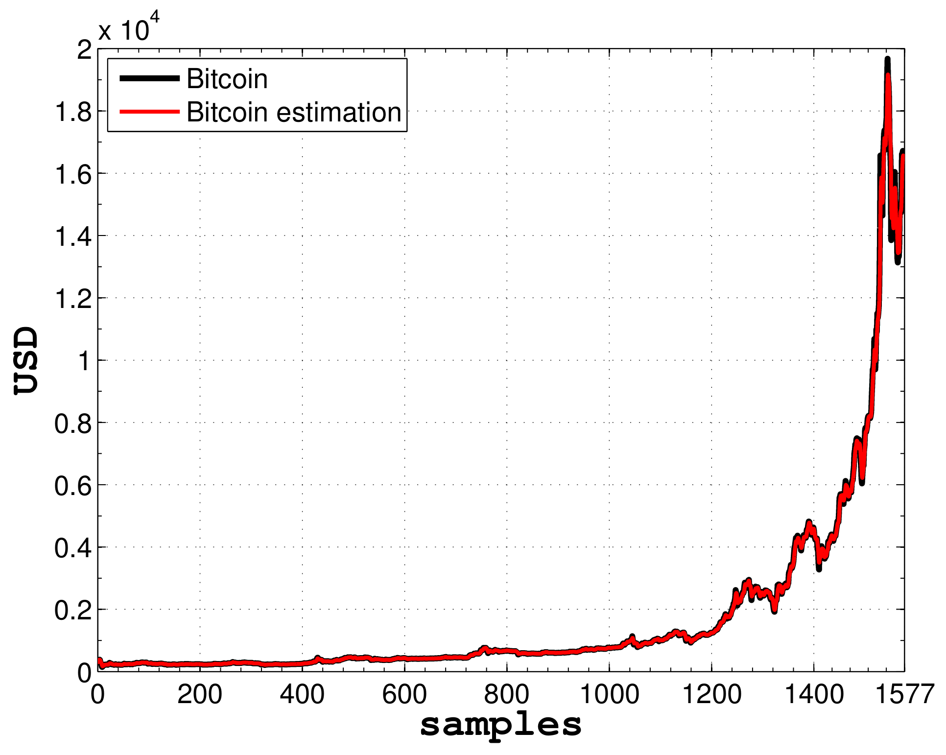
Bitcoin is the longest running and best known cryptocurrency in the world. It was released as open source in 2009 by the anonymous Satoshi Nakamoto. Bitcoin serves as a decentralized medium of digital exchange, with transactions verified and recorded in a public distributed ledger (the blockchain) without the need for a trusted record keeping authority or central intermediary. Hereafter, we will use the proposed spectral observer for fitting the historical Bitcoin market close data every 1000 [min]. The records were downloaded from the website: https://www.kaggle.com/neelneelpurk/bitcoin/data.

The observer to perform the estimation was tuned with $\lambda =1$. The order of the series was set $n=20$, i.e., $N=40$. The frequency step was set $\omega =10$ [rad/s]. The step time to perform the estimation in Simulink was set $\Delta t=0.01$ [s] and the used solver was ODE8.

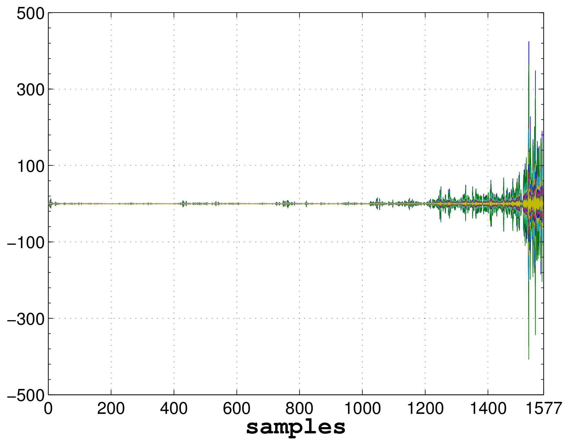
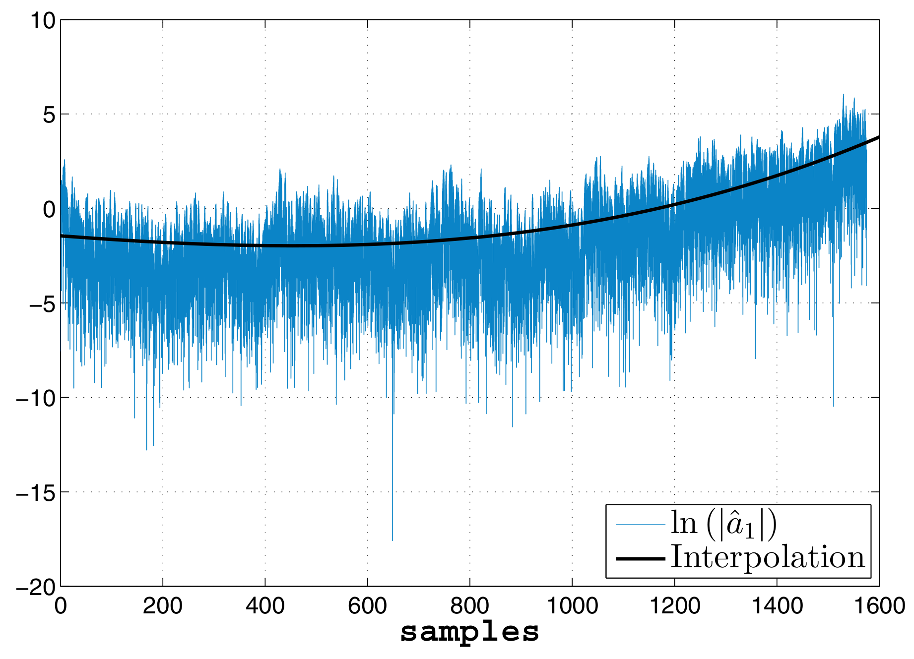
In Figure 7, the Bitcoin fitting performed by the spectral observer is shown. Figure 8 shows the estimated coefficients which are not constant and look as if they were enveloped by exponential functions. In order to have a model that represents the behavior of the Bitcoin in the specified interval, we can fit each coefficient by means of polynomials after calculating the natural logarithm of each one. In Figure 9, $\ln \left(\right|a_1\left|\right)$ is plotted versus a cubic polynomial calculated to interpolate it.

$$\ln \left(\right|a_1\left|\right)=1.2\times {10}^{-9}{t}^3+1.5\times {10}^{-6}{t}^2-0.0021t-1.4,$$

(16)

We can perform the same procedure for each coefficient to obtain a series with the following form:

$$\begin{array}{cc}\hfill \widehat{y}\left(t\right)=& \left(e^{\left|\right({\alpha }_{c1}{t}^3+{\beta }_{c1}{t}^2+{\gamma }_{c1}t+{\delta }_{c1}\left)\right|}\right)\cos \left(\omega t\right)+\left(e^{\left|\right({\alpha }_{s1}{t}^3+{\beta }_{s1}{t}^2+{\gamma }_{s1}t+{\delta }_{s1}\left)\right|}\right)\sin \left(\omega t\right)\hfill \\ \hfill +& \left(e^{\left|\right({\alpha }_{c2}{t}^3+{\beta }_{c2}{t}^2+{\gamma }_{c2}t+{\delta }_{c2}\left)\right|}\right)\cos \left(2\omega t\right)+\left(e^{\left|\right({\alpha }_{s2}{t}^3+{\beta }_{s2}{t}^2+{\gamma }_{s2}t+{\delta }_{s2}\left)\right|}\right)\sin \left(2\omega t\right)\hfill \\ \hfill +& \dots +\left(e^{\left|\right({\alpha }_{cn}{t}^3+{\beta }_{cn}{t}^2+{\gamma }_{cn}t+{\delta }_{cn}\left)\right|}\right)\cos \left(n\omega t\right)+\left(e^{\left|\right({\alpha }_{sn}{t}^3+{\beta }_{sn}{t}^2+{\gamma }_{sn}t+{\delta }_{sn}\left)\right|}\right)\sin \left(n\omega t\right)\hfill \end{array}$$

(17)

where ${\alpha }_{ck}$, ${\beta }_{ck}$, ${\gamma }_{ck}$, ${\delta }_{ck}$, ${\alpha }_{sk}$, ${\beta }_{sk}$, ${\gamma }_{sk}$, ${\delta }_{sk}$ are the coefficients of the polynomial that approximates the natural logarithms of the coefficients.

3.5. Example 5: Estimation of the Input Force on a Duffing Oscillator

One of the advantages of the proposed spectral observer is its structure, which is a chain of integrators expressed in state-space representation. Such a structure permits to couple the observer to dynamic models, also expressed in state variables, that represent physical systems for control or estimation purposes. With this in mind, we present an example to show how the spectral observer can be coupled to the model of a given system, even with nonlinear structure such as the Duffing oscillator, in order to estimate an exogenous input affecting its behavior.

The Duffing oscillator is expressed by the following equation:

$$\ddot{x}\left(t\right)+\delta \dot{x}\left(t\right)+\alpha x\left(t\right)+\beta x^3\left(t\right)=u\left(t\right)$$

(18)

where $x\left(t\right)$ is the displacement, which is assumed as available in this example, $\dot{x}\left(t\right)$ is the velocity and $\ddot{x}\left(t\right)$ is the acceleration. In addition, $\delta$, $\alpha$ and $\beta$ are parameters, which in this example are assumed to be known. Finally, $u\left(t\right)$ is an external force, which is unknown and can be estimated by using our proposed observer. To achieve this goal, the following steps need to be executed.

Step 1. Equation (18) must be set in state-space representation. To execute this step, we define $x_1\left(t\right)=x\left(t\right)$ and $x_2\left(t\right)=\dot{x}\left(t\right)$ as the state variables, such that we obtain the following equation system:

$$\begin{array}{cc}\hfill {\dot{x}}_1\left(t\right)& =x_2\left(t\right),\hfill \\ \hfill {\dot{x}}_2\left(t\right)& =-\delta x_2\left(t\right)-\alpha x\left(t\right)-\beta x^3\left(t\right)+u\left(t\right),\hfill \\ \hfill y\left(t\right)& =x_1\left(t\right).\hfill \end{array}$$

(19)

If the Liénard transform [13] is applied to system (18) in order to set it in a more appropriate form for estimation purposes [14], it becomes

$$\begin{array}{cc}\hfill {\dot{x}}_1\left(t\right)& =x_2\left(t\right)-\delta x_1\left(t\right),\hfill \\ \hfill {\dot{x}}_2\left(t\right)& =-\alpha x_1\left(t\right)-\beta x_1^3\left(t\right)+u\left(t\right),\hfill \end{array}$$

(20)

Step 2. Since $u\left(t\right)$ is unknown and needs to be estimated, we propose its estimation by using a spectral observer with $n=1$. Therefore, we coupled in cascade equation system (18) with equation system (4) as follows:

$$\begin{array}{cc}\hfill {\dot{x}}_1\left(t\right)& =x_2\left(t\right)-\delta x_1\left(t\right),\hfill \\ \hfill {\dot{x}}_2\left(t\right)& =-\alpha x_1\left(t\right)-\beta x_1^3\left(t\right)+{\nu }_1\left(t\right),\hfill \\ \hfill {\dot{\nu }}_1\left(t\right)& ={\nu }_2\left(t\right),\hfill \\ \hfill {\dot{\nu }}_2\left(t\right)& =-{\omega }^2{\nu }_1\left(t\right),\hfill \\ \hfill y\left(t\right)& =x_1\left(t\right),\hfill \end{array}$$

(21)

where ${\nu }_1\left(t\right)=u\left(t\right)$, i.e., it is the force to be estimated.

System (21) can be set in the following form:

$$\begin{array}{cc}\hfill \underset{\dot{\xi }\left(t\right)}{\underbrace{\left(\begin{array}{c}{\dot{x}}_1\left(t\right)\\ {\dot{x}}_2\left(t\right)\\ {\dot{\nu }}_1\left(t\right)\\ {\dot{\nu }}_2\left(t\right)\end{array}\right)}}& =\underset{A}{\underbrace{\left(\begin{array}{cccc}0& 1& 0& 0\\ 0& 0& 1& 0\\ 0& 0& 0& 1\\ 0& 0& -{\omega }^2& 0\end{array}\right)}}\underset{\xi \left(t\right)}{\underbrace{\left(\begin{array}{c}{x}_1\left(t\right)\\ x_2\left(t\right)\\ {\nu }_1\left(t\right)\\ {\nu }_2\left(t\right)\end{array}\right)}}+\underset{\phi \left(\xi \right(t\left)\right)}{\underbrace{\left(\begin{array}{c}-\delta y\left(t\right)\\ -\alpha y\left(t\right)-\beta y^3\left(t\right)\\ 0\\ 0\end{array}\right),}}\hfill \end{array}$$

(22)

$$\begin{array}{cc}\hfill y\left(t\right)& =\left[1000\right]\xi \left(t\right)=C\xi \left(t\right)=x_1\left(t\right),\hfill \end{array}$$

(23)

which according to [15] is uniformly observable. Therefore, a state observer expressed as $\widehat{\dot{\xi }}\left(t\right)=A\widehat{\xi \left(t\right)}+\phi (\widehat{\xi \left(t\right)})+K(x_1\left(t\right)-{\widehat{\xi }}_1\left(t\right))$ can be designed for system (22), where K can be calculated by means of Equation (14).

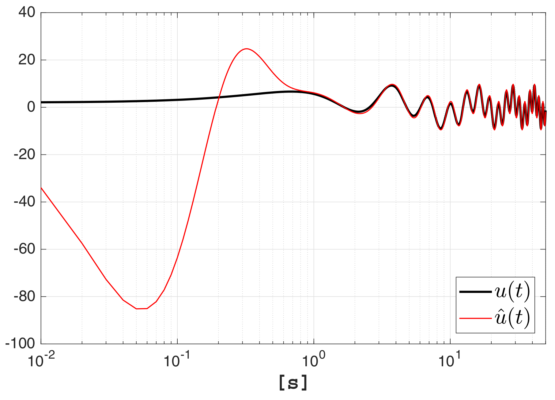
For the simulation, the paramaters of the Duffing oscillator were set: $\alpha =1$, $\beta =1$ and $\delta =0.3$; and their initial conditions were set $x\left(0\right)=[-1-5]$. The force applied to the oscillator was $u\left(t\right)=2\cos \left(2t\right)+5\sin \left(2t\right)+4\sin \left(0.5t\right)$. The observer was tuned with $\lambda =10$, $\omega =1$ [rad/s] and their initial conditions were fixed as $\widehat{\xi }\left(0\right)=\left[0000\right]$. Finally, the used solver was ODE 3 with a step time $\Delta t=0.01$ [s]. The results of the estimation are shown in Figure 10, which particularly presents a comparison between the force and its estimation. Notice that the estimation converges to the force in 1 [s].

4. Comparative Analysis Vis-à-Vis the STFT

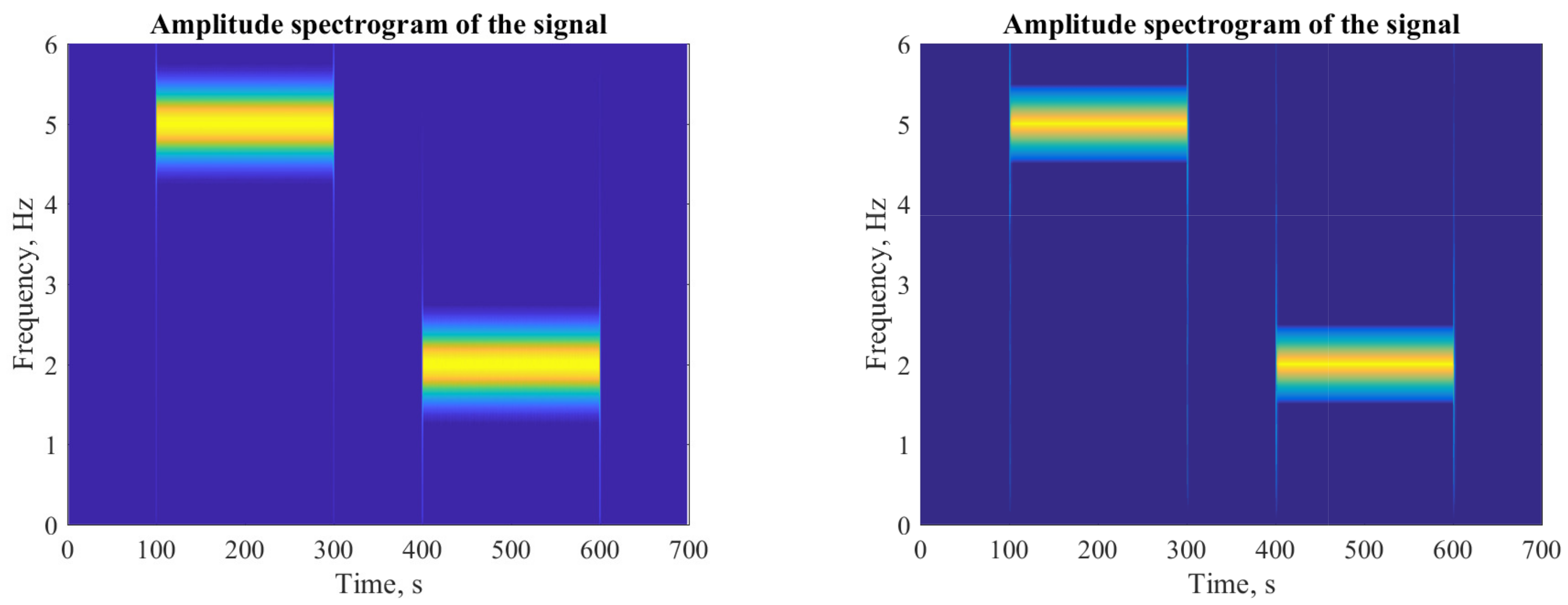
A spectral observer can be used to determine the frequency content of local sections of a signal as it changes over time. The classic technique for performing this task is the Short Time Fourier Transform, which is the Fourier Transform with a suitable chosen windowing function. Ensuing, we present an example to compare the results of using the STFT with the results provided by the spectral observer. For this purpose, we used the MATLAB${}^{\copyright }$ codes created by Hristo Zhivomirov to compute STFT and its inverse [16]. The signal analyzed was

$$s\left(t\right)=\left\{\begin{array}{c}00\le t<100\left[s\right]\hfill \\ \sin \left(10\pi t\right)0\le t<300\left[s\right]\hfill \\ 0300\le t<400\left[s\right]\hfill \\ \sin \left(4\pi t\right)400\le t<600\left[s\right]\hfill \\ 0600\le t<700\left[s\right]\hfill \end{array}\right.$$

(24)

sampled at 1000 [Hz]. To compute the STFT by using the code of Zhivomirov, the following parameters were set: ${\tau }_w=2^8$ [s] as the window length, $h={\tau }_w/4$ [s] as the hop size and $n_{fft}=2^{10}$ as the number of FFT points. The tuning of the spectral observer was done by setting $n=10$, $\lambda =1$, $\omega =\pi$ [rad/s] and $\widehat{\nu }\left(0\right)=0$. The solver used for the numerical solution was ODE4 (Runge-Kutta) with a fixed step size $\Delta t=0.01$ [s]. The spectrograms that were produced by the STFT and the spectral observer, respectively, are presented in Figure 11. To construct the observer spectrogram, we computed de magnitude of each harmonic by means of the following equation:

$$|A_k|=\sqrt{a_k+b_k}.$$

(25)

On the one hand, since $n=10$, the resulting vector containing the magnitude of each harmonic was $A=\left[A_1{A}_2{A}_3{A}_4{A}_5{A}_6{A}_7{A}_8{A}_9{A}_{10}\right]$. On the other hand, since the angular frequency step was chosen $\omega =\pi$ [rad/s], the resulting frequency vector was $f=\left[0.511.522.533.544.55\right]$ [Hz]. Then, the spectrogram resulted of plotting f versus A.

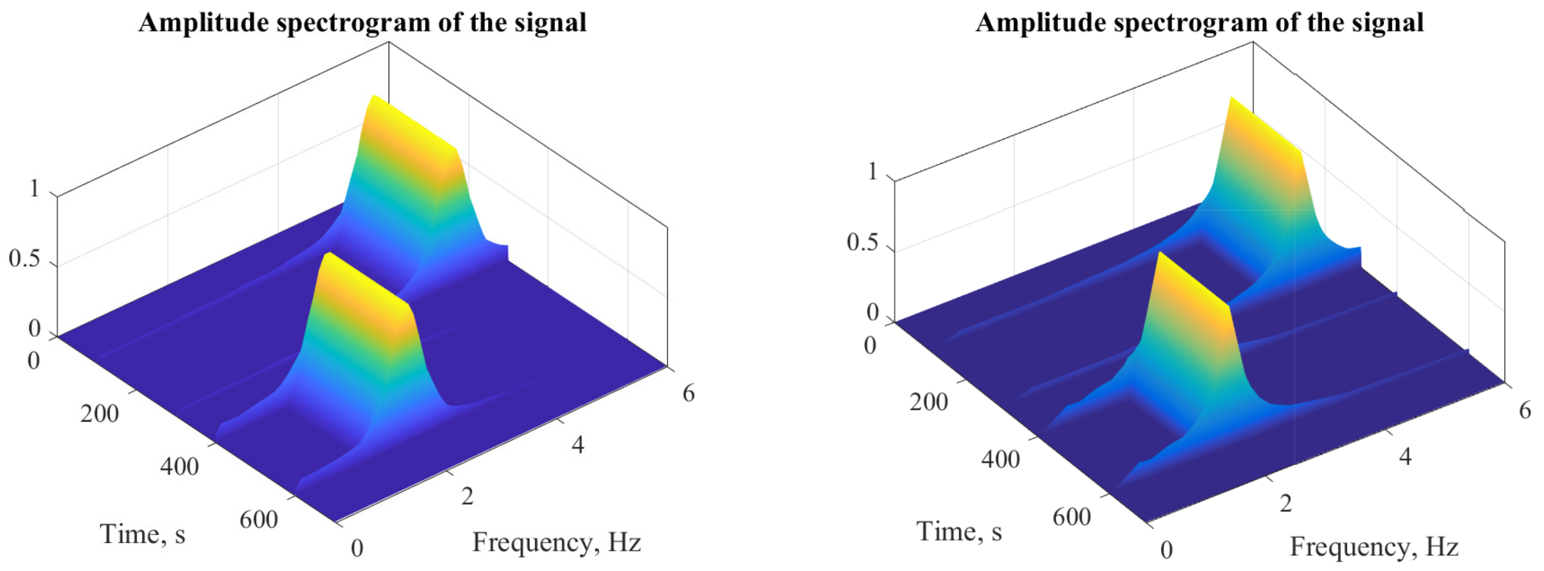
Notice that the spectrogram generated by using the spectral observer presents a better frequency resolution with respect to the spectral observer. This fact can be better appreciated in Figure 12. However, this does not mean that the observer’s performance is superior, since it is well known that the frequency resolution can be improved by widening the time window length of the STFT, even if this widening implies a decreasing of the time resolution. In the case of the spectral observer, the frequency resolution is adjusted by manipulating the parameter $\lambda$.

It is necessary to point out here that both the frequency resolution and the time resolution do not only depend on the parameters $\tau$ and $\lambda$, also the parameters h y $n_{fft}$ used in the STFT algorithm and $\omega$ and n used in the spectral observer, play an important factor; nevertheless, the adjustment of these parameters directly affects in the computational burden and the amount of data to be processed.

5. Results and Discussion

We have introduced an algorithm to reconstruct signals at the same time that their frequency components are calculated: a new spectral observer. In order to show its applicability, we have presented some examples, which in addition, have allowed us to glimpse some advantages and disadvantages of its use. Firstly, we found the following benefits: (1) The structure of the observer, as a chain of integrators, is very adequate for control and parameter estimation purposes; (2) The signal is progressively incorporated at each iteration; (3) The operations required for the observer implementation are with real numbers, which simplifies its programming in single-board computers; (4) The gain of the observer can be easily computed by means of a simple numerical algorithm; (5) The convergence of the observer is exponential, this means that the convergence period can be adjusted by means of a unique parameter $\lambda$, which is a clear advantage with respect to other well-known algorithms such as the proposed in [17], where the convergence period cannot be manipulated by a unique parameter. However, there are some drawbacks that we have found for the proposed observer. (1) The computational cost can be high for a small frequency resolution; (2) The algorithm must be complemented with a methodology to choose $\omega$ and $\lambda$ in order to obtain the best estimation.

To conclude the discussion, it is necessary to emphasize that the spectral observer is an algorithm that, like the STFT, can be used to perform a frequency-time analysis of a frequency varying signal by computing the Fourier Transform (FT) during time intervals. However, there are some differences to remark. (a) The STFT requires operations with complex numbers, the spectral observer does not; (b) The spectral observer computes the FT and its inverse at the same time, which is a clear bonus, because in case of using a recursive STFT we only get the FT, if we want to recover the reconstructed signal, we must compute the Inverse Short Fourier Transform.

6. Conclusions

In this paper, we presented the design of a novel spectral observer, which can be used to approximate periodical and non-periodical signals via state estimation. To design the spectral observer, we constructed a synthetic system in state space representation from the Fourier series. We presented some application examples to reconstruct periodical signals but also a well-know non-periodical one such as the price of the Bitcoin from its genesis. Some important aspects were not discussed in this article that require a deeper analysis, such as a comparison between the computational burden of the spectral observer and that of the Fourier Transform or an analysis of the spectral observer vis-à-vis perturbations and noise. These aspects must be treated in a continuation of this research work.

References

- Hostetter, G.H. Recursive discrete Fourier transformation. IEEE Trans. Acoust. Speech Signal Proc. 1980, 28, 184–190. [Google Scholar] [CrossRef]
- Bitmead, R.R.; Tsoi, A.C.; Parker, P.J. A Kalman filtering approach to short-time Fourier analysis. IEEE Trans. Acoust. Speech Signal Proc. 1986, 34, 1493–1501. [Google Scholar] [CrossRef]
- Orosz, G.; Sujbert, L.; Peceli, G. Spectral observer with reduced information demand. In Proceedings of the 2008 IEEE Instrumentation and Measurement Technology Conference, Victoria, BC, Canada, 12–15 May 2008; pp. 2155–2160. [Google Scholar]
- Na, J.; Yang, J.; Wu, X.; Guo, Y. Robust adaptive parameter estimation of sinusoidal signals. Automatica 2015, 53, 376–384. [Google Scholar] [CrossRef]
- Bitmead, R.R. On recursive discrete Fourier transformation. IEEE Trans. Acoust. Speech Signal Proc. 1982, 30, 319–322. [Google Scholar] [CrossRef]
- Torres, L.; Gómez-Aguilar, J.; Jiménez, J.; Mendoza, E.; López-Estrada, F.; Escobar-Jiménez, R. Parameter identification of periodical signals: Application to measurement and analysis of ocean wave forces. Digit. Signal Proc. 2017, 69, 59–69. [Google Scholar] [CrossRef]
- Dash, P.K.; Khincha, H. New algorithms for computer relaying for power transmission lines. Electr. Mach. Power Syst. 1988, 14, 163–178. [Google Scholar] [CrossRef]
- Houmb, O.; Overvik, T. Some applications of maximum entropy spectral estimation to ocean waves and linear systems response in waves. Appl. Ocean Res. 1981, 3, 154–162. [Google Scholar] [CrossRef]
- Blödt, M.; Chabert, M.; Regnier, J.; Faucher, J. Mechanical load fault detection in induction motors by stator current time-frequency analysis. IEEE Trans. Ind. Appl. 2006, 42, 1454–1463. [Google Scholar] [CrossRef]
- Benbouzid, M.E.H.; Vieira, M.; Theys, C. Induction motors’ faults detection and localization using stator current advanced signal processing techniques. IEEE Trans. Power Electron. 1999, 14, 14–22. [Google Scholar] [CrossRef]
- Busawon, K.; Farza, M.; Hammouri, H. A simple observer for a class of nonlinear systems. Appl. Math. Lett. 1998, 11, 27–31. [Google Scholar] [CrossRef]
- Engelberg, S. Edge detection using Fourier coefficients. Am. Math. Mon. 2008, 115, 499–513. [Google Scholar] [CrossRef]
- Liénard, A. Étude des oscillations entretenues. Revue Générale de l’Électricité 1928, 23, 901–912. [Google Scholar]
- Torres, L.; Verde, C.; Vázquez-Hernández, O. Parameter identification of marine risers using Kalman-like observers. Ocean Eng. 2015, 93, 84–97. [Google Scholar] [CrossRef]
- Hammouri, H. Uniform observability and observer synthesis. In Nonlinear Observers and Applications; Besançon, G., Ed.; Springer: Berlin, Germany, 2007; pp. 35–70. [Google Scholar]
- Zhivomirov, H. Short-Time Fourier Transformation (STFT) with Matlab Implementation. Available online: https://www.mathworks.com/matlabcentral/fileexchange/45197-short-time-fourier-transformation--stft--with-matlab-implementation (accessed on 27 April 2018).
- Kušljević, M.D.; Tomić, J.J. Multiple-resonator-based power system Taylor-Fourier harmonic analysis. IEEE Trans. Instrum. Meas. 2015, 64, 554–563. [Google Scholar] [CrossRef]
Figure 1.
Schema of the reconstruction of a signal by using the spectral observer.
Figure 2.
Example 1. Estimated coefficients.
Figure 3.
Example 2. (a) Square wave reconstruction and (b) Estimated coefficients.
Figure 4.
Example 2. (a) Triangular wave reconstruction and (b) Estimated coefficients.
Figure 5.
Variations of parameter .
Figure 6.
Example 3. (a) Signal reconstruction and (b) Estimated coefficients.
Figure 7.
Example 4. Bitcoin fitting.
Figure 8.
Example 4. Estimated coefficients.
Figure 9.
Example 4. vs. interpolation.
Figure 10.
Example 5. Force estimation.
Figure 11.
(a) STFT spectrogram (b) Spectral observer spectrogram.
Figure 12.
© 2018 by the authors. Licensee MDPI, Basel, Switzerland. This article is an open access article distributed under the terms and conditions of the Creative Commons Attribution (CC BY) license (http://creativecommons.org/licenses/by/4.0/).
Share and Cite
MDPI and ACS Style
Torres, L.; Jiménez-Cabas, J.; Gómez-Aguilar, J.F.; Pérez-Alcazar, P. A Simple Spectral Observer. Math. Comput. Appl. 2018, 23, 23. https://doi.org/10.3390/mca23020023
AMA Style
Torres L, Jiménez-Cabas J, Gómez-Aguilar JF, Pérez-Alcazar P. A Simple Spectral Observer. Mathematical and Computational Applications. 2018; 23(2):23. https://doi.org/10.3390/mca23020023
Chicago/Turabian StyleTorres, Lizeth, Javier Jiménez-Cabas, José Francisco Gómez-Aguilar, and Pablo Pérez-Alcazar. 2018. "A Simple Spectral Observer" Mathematical and Computational Applications 23, no. 2: 23. https://doi.org/10.3390/mca23020023