The Construction of a Model-Robust IV-Optimal Mixture Designs Using a Genetic Algorithm

Abstract

Among the numerous alphabetical optimality criteria is the IV-criterion that is focused on prediction variance. We propose a new criterion, called the weighted IV-optimality. It is similar to IV-optimality, because the researcher must first specify a model. However, unlike IV-optimality, a suite of “reduced” models is also proposed if the original model is misspecified via over-parameterization. In this research, weighted IV-optimality is applied to mixture experiments with a set of prior weights assigned to the potential mixture models of interest. To address the issue of implementation, a genetic algorithm was developed to generate weighted IV-optimal mixture designs that are robust across multiple models. In our examples, we assign models with p parameters to have equal weights, but weights will vary based on varying p. Fraction-of-design-space (FDS) plots are used to compare the performance of an experimental design in terms of the prediction variance properties. An illustrating example is presented. The result shows that the GA-generated designs studied are robust across a set of potential mixture models.

1. Introduction

Industrial product formulations (e.g., food processing, chemical formulations, textile fibers, and pharmaceutical drugs) frequently involve the blending of multiple mixture components. Mixture experiments form a special class of response surface experiments in which the product under investigation is comprised of several components. In this research, we assume that the response of interest is a function only of the proportions of the components that are present in the mixture. The levels of the q experimental factors (x_i; i = 1, 2, …, q) in a mixture experiment are component proportions. Thus, each x_i is between zero and one, and the sum of the q component proportions is one. Under these conditions, the experimental region involving q proportions is a regular q − 1-dimensional simplex. Typically, there are also single-component constraints (SCCs) defined by lower L_i and upper U_i bounds on the component proportions:

$$0\le L_i\le x_i\le U_i\le 1\hspace{1em} \mathrm{for} i=1,2,\dots ,q.$$

(1)

If SCCs are imposed on the component proportions, the experimental region will now be an irregularly shaped polyhedron within the simplex. For a general review of the design and analysis of mixture experiments, see [1,2].

When the mixture region is a simplex, the standard mixture designs such as simplex lattice and simplex centroid designs are often suitable for implementation. However, they are not applicable in situations involving SCCs. When SCCs exist, an extreme vertices design (McLean and Anderson [3]) is one possibility. However, these designs may be very inefficient with respect to prediction variance properties. To improve the prediction variance properties, an algorithmically generated design focused on optimizing an optimality design criterion is commonly used. Optimal designs, however, are, in general, optimal only for a specified model. Numerous approaches have been developed for constructing optimal designs, such as ACED [4], XVERT [5], CONSIM [6], Fedorov [7], DETMAX [8], exchange algorithms [9,10], and genetic algorithms (GAs) [11,12,13,14,15]. GAs have the advantage of being adaptive search algorithms [14]. Recent applications of GAs provide alternative approaches to classic exchange-point algorithms to generate designs. Examples of using GAs to generate designs can be found in Borkowski [11], Heredia-Langner et al. [12,13], Park et al. [15], and Limmun et al. [16].

In this research, we develop and employ a GA that extends the work in Limmun et al. [16] that focused on a single model when constructing an IV-optimal design where the experimental region was an irregularly shaped polyhedral region that is a subspace of a simplex. Their procedure offered a degree of flexibility in its way of constructing designs that allowed it to overcome restrictions that may limit the applicability of other algorithms. The first aim of our research is to consider model misspecification and introduce a weighted IV-optimality criterion determined over a set of potential mixture models, and it will serve to address our second aim: develop a design-generating GA using weighted IV-optimality as its objective function.

The rest of this paper is organized as follows. In Section 2, the Scheffé mixture models and relevant theory relating to mixture experiments of interest are reviewed, and weighted IV-efficiency is defined. Section 3 includes a brief introduction to GAs for constructing designs and an illustration of the steps used in our GA. In Section 4, the proposed scheme is demonstrated with examples, and with concluding statements in Section 5.

2. The Mixture Model and Design Optimality

2.1. Notation and Models

The most common forms of mixture models are the Scheffé (canonical) polynomials. For example, the Scheffé linear model is given by

$$y={\displaystyle \sum }_{i=1}^q{\beta }_i{x}_i+\epsilon$$

(2)

and the Scheffé quadratic model is given by

$$y={\displaystyle \sum }_{i=1}^q{\beta }_i{x}_i+{\displaystyle \sum }_{i=1}^{q-1}{\displaystyle \sum }_{j=i+1}^q{\beta }_{ij}{x}_i{x}_j+\epsilon .$$

(3)

In these models, $y$ is the response variable; each ${\beta }_i$ coefficient represents the expected response when the proportion of the i-th component equals unity; each ${\beta }_{ij}$ coefficient represents the nonlinear blending properties of the i-th and the j-th component proportions, and $\epsilon$ is a random error. In this paper, we focus on the Scheffé quadratic model mixture model and possible model misspecification.

The Scheffé mixture models are linear models and can be expressed in the matrix form as

$$\mathit{y}=\mathit{X}\mathit{\beta }+\mathit{\epsilon }$$

(4)

where $\mathit{y}={\left(y_1,y_2,\dots ,y_n\right)}^{\prime }$ is the response vector, $\mathit{X}$ is the $N\times p$ model matrix with columns associated with the $p$ model terms (such as linear and cross-products terms), $\mathit{\beta }$ is the $p\times 1$ vector of model parameters, and $\mathit{\epsilon }={\left({\epsilon }_1,{\epsilon }_2,\dots ,{\epsilon }_n\right)}^{\prime }$ is the vector of random errors associated with natural variation of $\mathit{y}$ around the underlying surface assumed to be independent and identically normally distributed with zero mean and variance ${\sigma }^2{\mathit{I}}_n$. The prediction properties of a design, specifically the scaled prediction variance, is dependent on the chosen model through model matrix $\mathit{X}$. The scaled prediction variance $v\left({\mathit{x}}_{\mathbf{0}}\right)$ is defined as

$$v\left({\mathit{x}}_{\mathbf{0}}\right)=\frac{N\mathrm{Var}\left(\widehat{y}\left(\mathit{x}\right)\right)}{{\sigma }^2}=N{\mathit{x}}_{\mathbf{0}}^{\prime }{\left({\mathit{X}}^{\prime }\mathit{X}\right)}^{-\mathbf{1}}{\mathit{x}}_{\mathbf{0}}$$

(5)

where ${\mathit{x}}_{\mathbf{0}}^{\prime }$ is the expansion of a mixture $\mathit{x}=\left(x_1,x_2,\dots ,x_q\right)$ to vector form corresponding to the $p$ columns of $\mathit{X}$; $N$ is the design size, which penalizes prediction variances for larger designs, and $\mathrm{Var}\left(\widehat{y}\left(\mathit{x}\right)\right)$ is the variance of the estimated response at $\mathit{x}$. For example, if there are three components and the model is the Scheffé quadratic model, then $\mathit{x}=\left(x_1,x_2,x_3\right)$, ${{\mathit{x}}_{\mathbf{0}}}^{\prime }=\left(x_1,x_2,x_3,x_1{x}_2,x_1{x}_3,x_2{x}_3\right)$, and $\mathit{X}$ is an $N\times 6$ model matrix.

2.2. Optimality Criteria

Design optimality criteria are single valued criteria that represent different variance or parameter estimation properties of a design. Several criteria have been advanced with the purpose of constructing and comparing and designs. Four commonly used optimality criteria are the D, A, G, and IV criteria. These four criteria are functions of the information matrix $\left({\mathit{X}}^{\prime }\mathit{X}\right)$ for a given design. The D and A criteria are focused on parameter estimation, while G and IV criteria are focused on the prediction variance. When a design is being considered for implementation, several of its properties can be evaluated by computing measures of design efficiency. Common D, A, G, and IV design optimality measures are

$$\mathrm{D}-\mathrm{efficiency}=\frac{100{\left|{\mathit{X}}^{\prime }\mathit{X}\right|}^{1/p}}{N},\hspace{1em}\mathrm{A}-\mathrm{efficiency}=\frac{100p}{\mathrm{trace}[N{\left({\mathit{X}}^{\prime }\mathit{X}\right)}^{-1}]}$$

$$\mathrm{G}-\mathrm{efficiency}=\frac{100p}{\underset{x\epsilon \chi }{\max } \left[v\left({\mathit{x}}_{\mathbf{0}}\right)\right] },\hspace{1em}\mathrm{IV}-\mathrm{efficiency}=\frac{V}{{\int }_{\chi }v\left({\mathit{x}}_{\mathbf{0}}\right)d{x}_{1}d{x}_2\dots d{x}_q}$$

where $\chi$ is the design space and $V$ is the volume of $\chi$. The D and A criteria are the simplest to handle computationally, and they were the criteria considered in the earliest design generating algorithms (e.g., exchange algorithms). Because designs with high IV or G efficiencies also tend to have good D- and A-efficiencies, this paper will focus on designs that minimize the average prediction variance (i.e., minimize the denominator in the IV-efficiency over the entire experimental region). Designs that minimize the IV-optimality criterion include the IV-optimal design, the Q-optimal design [17], the V-optimal design [18], and the I-optimal design [19,20].

In a review of software approaches to evaluating average prediction variances (APVs), Borkowski [21] showed that it is common for software packages to estimate the APV = ${\int }_{\chi }v\left({\mathit{x}}_{\mathbf{0}}\right)d{x}_{1}d{x}_2\dots d{x}_q$ by taking the sample mean of $v\left({\mathit{x}}_{\mathbf{0}}\right)$ over a fixed set of points (e.g., the candidate set for an exchange algorithm). He demonstrated that estimation of the APV based instead on a random set of evaluation points is unbiased and superior to estimation based on a fixed set of evaluation points. This is one flaw in using software using exchange algorithms to generate IV-optimal designs: the estimated APV is an overestimation of the integral. In our proposed GA, the APV measure is calculated by averaging $v\left({\mathit{x}}_{\mathbf{0}}\right)$ over a random set of points and will provide an unbiased estimate of the IV-optimality criterion. Additionally, the variability of the estimator will decrease as the size of the random evaluation set increases. In this paper, we use 5000 random points in the evaluation set. Several authors have provided results for the IV-optimal designs, including Borkowski [11], Syafitri et al. [20], and Coetzer and Haines [22]. Further details on the motivation and uses of the optimality criteria can be found in Box and Draper [23], Atkinson et al. [18], and Fedorov [7].

2.3. Weighted IV-Optimality

In this paper, we develop and propose the weighted IV-efficiency, which is defined as

$$\mathrm{Weighted} \mathrm{IV}-\mathrm{efficiency}={{\displaystyle \sum }}_{i=1}^r{w}_{i}I{V}_i$$

(6)

where $I{V}_i=\frac{V}{{\int }_{\chi }v\left({\mathit{x}}_{\mathbf{0}}\right) d{x}_1 d{x}_2\dots d{x}_q}$ is the IV-efficiency for model $i$, $\chi$ is the design space, $V$ is the volume of $\chi$, $N$ is the number of design points, $r$ is the number of reduced models for a given full model, and w_i is the weight for model i.

In terms of design generation, the goal is to use weighted IV-optimality to find a set of points that will minimize the weighted average of the average of the scaled prediction variance over the design region across a set of reduced models. Practically speaking, the goal is to generate a design that protects against having a final model with poor prediction variance properties. Similar to finding an IV-optimal design, the researcher must specify a model. This serves as the “full” model when we consider the weighted IV-optimality. However, unlike IV-optimality, a suite of “reduced” models are also proposed if the full model is misspecified via over-parameterization. Examining Equation (6), note that weighted IV-optimality is not restricted to a particular full model nor is it restricted to mixture models. It easily generalizes to other response surface designs and the associated models that can be fitted by those designs.

The experimenter has the freedom to choose the weighting factors for the full model, the most parsimonious or smallest model, as well as all other intermediate models. To exemplify the use of weighted IV-optimality, a “full” quadratic mixture model and a “smallest” linear mixture model will be considered.

Although there are numerous ways to assign weights in the weighted optimality criterion, in this paper, we assume (i) that not all models should be weighted equally and (ii) that only models having an equal number of model parameters receive equal weight. Here are the reasons for assuming (i) and (ii). Before running the experiment, the experimenter believes that the full model may be the most appropriate, so he/she chooses the maximum weighting factor for the full model. In the analysis phase, however, the full model might be inappropriate because of misspecification due to overparameterization. Thus, it seems reasonable that the weights be reduced as we move further away from the full (or the experimenter’s most likely a priori) model via model reduction, and stop with the smallest weight assigned to the model with the fewest number of parameters. We also treat each parameter as equally important under the assumption that the researcher has no prior knowledge or make an educated guess regarding which terms would most likely be removed if a model reduction occurs. Therefore, we assign uniform weights among all models resulting after removal of one term, and then assign a decreasing but uniform weight to all models resulting when two terms are moved, and so on. Therefore, models with more parameters have weights that reflect their greater importance relative to models with fewer parameters. For the proposed method of calculating a weighted IV-efficiency, it is necessary to have a complete enumeration of the set of subset models (reduced models) of interest. If an experimenter has justification for another weighting scheme, then it should certainly be implemented.

One specific weighting scheme consistent with (i) and (ii) above is to use weights for each reduced model based on the numbers of model parameters. Suppose model $i$ has $j$ parameters. The weight we assigned to model $i$ is then defined as

$$w_i=\frac{{\psi }_j}{m_j}$$

(7)

where ${\psi }_j$ is the $j\mathrm{th}$ weighting factor, and $j=q,q+1,\dots ,s-1,s$, where $q$ is the number of parameters of the linear mixture model in Equation (2); $s$ is the number of parameters of the quadratic model in Equation (3), and $m_j$ is the number of reduced models with $j$ parameters. The model $i$ weight $\left(w_i,i=1,2,\dots ,r\right)$ is nonnegative and the weights satisfy ${{\displaystyle \sum }}_{i=1}^r{w}_i=1$. The relative weighting factor for computing the weighting factors (supplied by the experimenter) is defined as

$$R=\frac{{\psi }_s}{{\psi }_q}.$$

(8)

In this paper, we assume that the experimenter weights the quadratic mixture model 100 times the weight to be assigned to the linear mixture model; therefore, we use $R$ = 100 as the relative weighting factor. The weighting factors are positive and subject to the restriction

$${\psi }_q+{\psi }_{q+1}+\dots +{\psi }_{s-1}+{\psi }_s=1.$$

(9)

There are $k$ equispaced levels of the weighting factor, and $k=s-q+1$ is the number of levels for a weighting factor. Therefore, the range of the weighting factor is defined as

$${\psi }_k={\psi }_s-{\psi }_q=R{\psi }_q-{\psi }_q=\left(R-1\right){\psi }_q.$$

(10)

The increment value of the weighting factor can be expressed as

$$INCR=\frac{{\psi }_k}{k-1}=\frac{\left(R-1\right){\psi }_q}{k-1}.$$

(11)

The values of the weighting factor can be represented as follows:

$${\psi }_{q+c} ={\psi }_q+cINCR;c=0,1,\dots ,k-1.$$

(12)

Again, the weighting factor must sum to one. The weighting factor can be rewritten in the form:

$${\displaystyle \sum }_{i=q}^s{\psi }_i=k{\psi }_q+\left(\begin{array}{c}k\\ 2\end{array}\right)INCR=1.$$

(13)

Therefore, the minimum weighting factor can be expressed as

$${\psi }_q=\frac{\left(k-1\right)INCR}{R-1}.$$

(14)

After simplifying, the increment value of the weighting factor is defined as

$$INCR=\frac{2\left(R-1\right)}{k\left(k-1\right)\left(R+1\right)}.$$

(15)

For example, suppose the full model is the quadratic mixture model with three component proportions. This model can be expressed as

$$E\left(y\right)={\beta }_1{x}_1+{\beta }_2{x}_2+{\beta }_3{x}_3+{\beta }_{12}{x}_1{x}_2+{\beta }_{13}{x}_1{x}_3+{\beta }_{23}{x}_2{x}_3.$$

There are 8 reduced models (the full model and the seven reduced models as shown in

Table 1. The set of reduced models the Scheffé quadratic model with three components.

Model	Terms in Model						p	ψj	wi
	${\mathit{x}}_1$	${\mathit{x}}_2$	${\mathit{x}}_3$	${\mathit{x}}_1{\mathit{x}}_2$	${\mathit{x}}_1{\mathit{x}}_3$	${\mathit{x}}_2{\mathit{x}}_3$
1st	1	1	1	1	1	1	6	0.4950	0.4950
2nd	1	1	1	0	1	1	5	0.3318	0.1106
3rd	1	1	1	1	0	1	5		0.1106
4th	1	1	1	1	1	0	5		0.1106
5th	1	1	1	0	0	1	4	0.1683	0.0561
6th	1	1	1	0	1	0	4		0.0561
7th	1	1	1	1	0	0	4		0.0561
8th	1	1	1	0	0	0	3	0.0049	0.0049

). A 1 or a 0 in any “Terms in Model” column represents the presence or absence of that term in the model, respectively. The column $p$ is the number of model parameters. Using 100 as the relative weighting factor, the increment value of the weighting factor is 0.1634. The weighting factor value and the weight for each model are shown in the ${\psi }_j$ and $w_i$ columns, respectively. If the 2nd, 3rd, and 4th models have five parameters, then $m_5=3$, and the 5-parameter model weighting factor ${\psi }_5$ = 0.3318 and the individual model weights $w_2,w_3$, and $w_4={\psi }_5$/3 = 0.1106.

3. Genetic Algorithms and Constructing IV-Optimal Mixture Designs

3.1. Development of the Genetic Algorithm

Heuristic optimization has been used to solve a variety of experimental design problems. One popular optimization algorithm that is based on the general principle of local improvement is the genetic algorithm (GA). The genetic algorithm was developed by John Holland in 1975 and was popularized through the work of Goldberg in 1989 [24]. Since then, GAs have been used to solve optimization problems for many applications because it is very efficient over a variety of search spaces. Bäck et al. [25] mention that GAs often yield excellent results when applied to complex optimization problems where other methods are either not applicable or turn out to be unsatisfactory. GAs have been successfully applied to experimental design problems using various optimality criteria. For an introduction to GAs, see Michaelewicz [26] and Haupt and Haupt [27].

A GA is a search and optimization technique developed by mimicking the evolutionary principles and the chromosomal processing in the natural selection. A GA takes an initial population of potential solutions to a problem (parent chromosomes). Through evolutionary reproduction operators, the current parent population then passes some of its properties (genes) to produce offspring chromosomes. A subset of the best parent and offspring is retained for the next generation, and the reproduction process is repeated for many generations until an acceptable chromosome has evolved. A GA uses an objective function as a measure of a chromosome’s fitness as a solution to the problem of interest. Although a GA is not guaranteed to find the global optimum in a finite number of generations, it is less likely to get trapped at a local optimum than traditional gradient-based search methods when the objective function is not smooth and generally well behaved.

GAs can be very useful for construction of a design when the optimality criterion (objective function) is difficult to work with and/or where there are constraints on the experimental region such as in mixture experiments. We now describe a GA used to generate optimal designs for a mixture experiment with single component constraints (SCCs) that is based on weighted IV-optimality, which extends and modifies the GA approach of Limmun et al. [16] who generated optimal designs for a specified mixture model. Throughout this research paper, we have encoded GA chromosomes using real-value encoding instead of another encoding (e.g., binary) because real-value encoding is easy to interpret, can be modified for many applications, and is flexible enough to allow for a unique representation for every variable.

A chromosome $C$ will represent a potential design (solution) and is encoded as an $N\times q$ matrix, where $N$ is the number of the design points, and $q$ is the number of mixture components. Each row in $C$ is a gene ${\mathit{x}}_{\mathit{i}}=\left[x_{i1} x_{i2}\dots x_{iq}\right]$ and represents one experimental mixture. The objective function $F$ measures a chromosome’s fitness as a solution to the function that we wish to optimize. That is, $F$ takes a chromosome as input and outputs an objective function value. Our GA’s objective function $F$ is a weighted IV-efficiency. The goal using a weighted IV-efficiency is to find a set of points that will minimize the weighted average of the scaled prediction variance throughout the entire experimental region for a set of reduced models representing possible model misspecification. Specifically, the goal is to find a design that maximizes objective function $F$ where

$$F={\displaystyle \sum }_{i=1}^r{w}_{i}I{V}_i$$

(16)

where $I{V}_i=\frac{V}{{\int }_{\chi }v\left({\mathit{x}}_{\mathbf{0}}\right)d{x}_{1}d{x}_2\dots d{x}_q}$ is the IV-efficiency for model $i$, $\chi$ is the design space, $V$ is the volume of $\chi$, $r$ is the number of reduced models for a given full model, and $w_i$ is the weight for model $i$. The GA that we employed includes several genetic operators. Prior to running a GA, the experimenter must specify the $r$ models of interest and the model weights $w_i$. The steps and operators in our GA are as follows:

Step 1

Specify the GA parameters: population size $\left(M\right)$, number of iterations $\left(I\right)$, selection method (elitism with random parent pairing), blending rate $\left({\alpha }_b\right)$, crossover rates $\left({\alpha }_{bc} \mathrm{and} {\alpha }_{wc}\right)$, and mutation rate $\left({\alpha }_m\right)$.

Step 2

Generate an initial population of $M$ chromosomes (mixture designs). We use the real-value encoding with four decimal places to encode each chromosome. Assume $M$ is odd. To generate the initial population, a random sample is first taken in a hypercube. Then each sampled point in a hypercube is mapped to the constrained mixture space by applying the function used by Borkowski and Piepel [28]. Each experimental mixture is recorded to four-decimal place accuracy.

Step 3

Calculate the IV-efficiency objective function $F$ for each chromosome in the initial population.

Step 4

Find the elite chromosome which is the chromosome that has the largest weighted IV-efficiency $F$. The remaining $M-1$ chromosomes are randomly paired for the reproduction process.

Step 5

Produce offspring of the next generation by using genetic operators: blending, between-parent crossover, within-parent crossover, and mutation. Larger values of genetic parameters are used for the early iterations and the smaller values of genetic parameters are used for the later.

Step 6

Calculate objective function $F$ for each parent/offspring pair. The fitter chromosome in the pair is retained for the next generation.

Step 7

Repeat Steps 5 and 6 for $I$ generations.

Step 8

Apply a local grid search to the best design to further improve objective function $F$ yielding the IV-optimal design. A local grid search searches designs in a small neighborhood of the best design. This is accomplished by perturbing the component proportions by small increments to search for further improvements in $F$. This continues until no further improvement is found.

3.2. Illustration: A Genetic Algorithm for Constructing an Optimal Mixture Design

To illustrate our algorithm, consider a three-component mixture $\left(q=3\right)$ with the goal of generating a weighted IV-optimal design having $N$ = 7 design points. We create an initial population of $M=5$ chromosomes $\left(C_1,C_2,C_3,C_4,C_5\right)$ each having 7 genes where the genes of each chromosome (mixture design) are drawn randomly from the mixture space. One possible realization of the initial population and the associated objective function values are presented in

Table 2. Initial population of five chromosomes.

${\mathit{C}}_1$			${\mathit{C}}_2$			${\mathit{C}}_3$			${\mathit{C}}_4$			${\mathit{C}}_5$
${\mathit{x}}_1$	${\mathit{x}}_2$	${\mathit{x}}_3$	${\mathit{x}}_1$	${\mathit{x}}_2$	${\mathit{x}}_3$	${\mathit{x}}_1$	${\mathit{x}}_2$	${\mathit{x}}_3$	${\mathit{x}}_1$	${\mathit{x}}_2$	${\mathit{x}}_3$	${\mathit{x}}_1$	${\mathit{x}}_2$	${\mathit{x}}_3$
0.6531	0.2958	0.0511	0.5242	0.2016	0.2742	0.5771	0.1605	0.2624	0.5160	0.1979	0.2861	0.6705	0.0536	0.2759
0.3612	0.2765	0.3623	0.5858	0.2007	0.2135	0.5229	0.1136	0.3635	0.6487	0.1443	0.2070	0.5256	0.0173	0.4571
0.5077	0.1156	0.3767	0.5367	0.2877	0.1756	0.7316	0.1828	0.0856	0.4404	0.0682	0.4914	0.4927	0.1614	0.3459
0.4479	0.1197	0.4324	0.5214	0.0236	0.455	0.4780	0.2241	0.2979	0.5488	0.2372	0.2140	0.4754	0.0946	0.4300
0.7274	0.0546	0.2180	0.3942	0.1999	0.4059	0.7514	0.2388	0.0098	0.6744	0.1869	0.1387	0.6723	0.0354	0.2923
0.6519	0.2764	0.0717	0.7271	0.1305	0.1424	0.7969	0.1201	0.0830	0.7693	0.2281	0.0026	0.5367	0.0700	0.3933
0.7612	0.2179	0.0209	0.7569	0.1026	0.1405	0.5422	0.2942	0.1636	0.5322	0.1513	0.3165	0.6342	0.1343	0.2315
F = 0.2050			F = 0.1344			F = 0.0848			F = 0.0400			F = 0.0285

. $C_1$ is the elite chromosome because it has the largest $F$ value. Next, the remaining four chromosomes are randomly paired for the reproduction process. Suppose that $\left(C_5,C_4\right)$ and $\left(C_2,C_3\right)$ are the randomly formed pairs. Applying the reproduction process to $C_5$ and $C_4$ yields offspring $C_5^{\ast }$ and $C_4^{\ast }$.

Table 3. Random deviates for probability tests on $C_5$ and $C_4$.

Blending	Between-Parent Crossover	Within-Parent Crossover		Mutation
Parent 1	Parent 1	Parent 1	Parent 2	Parent 1	Parent 2
0.9563	0.7198	0.2807	0.4561	0.8851	0.0049
0.5209	0.7448	0.5894	0.5453	0.9218	0.9710
0.0158	0.6830	0.0179	0.6338	0.1266	0.2420
0.6306	0.6609	0.1799	0.7857	0.0155	0.0400
0.1155	0.4510	0.6985	0.0769	0.3290	0.6497
0.6471	0.0017	0.6031	0.5732	0.8324	0.0840
0.8924	0.0509	0.9297	0.0095	0.6498	0.3173

contains a set of random uniform deviates for $C_5$ and $C_4$. Boldfacing indicates a probability test is passed (PTIP) at rates ${\alpha }_b,{\alpha }_{bc},{\alpha }_{wc}$ and ${\alpha }_m=0.02$, and that reproduction operation will be performed where ${\alpha }_b,{\alpha }_{bc},{\alpha }_{wc}$, and ${\alpha }_m$ represent the success probabilities of blending, between-parent crossover, within-parent crossover, and mutation, respectively.

The first generation is summarized in

Table 4. First generation reproduction for chromosomes $C_5$ and $C_4$.

After Blending						After between-Parent Crossover						After within-Parent Crossover						After Mutation
${\mathit{C}}_5^{\ast }$			${\mathit{C}}_4^{\ast }$			${\mathit{C}}_5^{\ast }$			${\mathit{C}}_4^{\ast }$			${\mathit{C}}_5^{\ast }$			${\mathit{C}}_4^{\ast }$			${\mathit{C}}_5^{\ast }$			${\mathit{C}}_4^{\ast }$
${\mathit{x}}_1$	${\mathit{x}}_2$	${\mathit{x}}_3$	${\mathit{x}}_1$	${\mathit{x}}_2$	${\mathit{x}}_3$	${\mathit{x}}_1$	${\mathit{x}}_2$	${\mathit{x}}_3$	${\mathit{x}}_1$	${\mathit{x}}_2$	${\mathit{x}}_3$	${\mathit{x}}_1$	${\mathit{x}}_2$	${\mathit{x}}_3$	${\mathit{x}}_1$	${\mathit{x}}_2$	${\mathit{x}}_3$	${\mathit{x}}_1$	${\mathit{x}}_2$	${\mathit{x}}_3$	${\mathit{x}}_1$	${\mathit{x}}_2$	${\mathit{x}}_3$
0.6705	0.0536	0.2759	0.5160	0.1979	0.2861	0.6705	0.0536	0.2759	0.5160	0.1979	0.2861	0.6705	0.0536	0.2759	0.5160	0.1979	0.2861	0.6705	0.0536	0.2759	0.4721	0.2999	0.2800
0.5256	0.0173	0.4571	0.6487	0.1443	0.2070	0.5256	0.0173	0.4571	0.6487	0.1443	0.2070	0.5256	0.0173	0.4571	0.6487	0.1443	0.2070	0.5256	0.0173	0.4571	0.6487	0.1443	0.2070
0.5239	0.2036	0.2725	0.4404	0.0682	0.4914	0.5239	0.2036	0.2725	0.4467	0.0600	0.4933	0.5225	0.2036	0.2739	0.4467	0.0600	0.4933	0.5225	0.2036	0.2739	0.4467	0.0600	0.4933
0.4754	0.0946	0.4300	0.5176	0.1950	0.2874	0.4754	0.0946	0.4300	0.5176	0.1950	0.2874	0.4754	0.0946	0.4300	0.5176	0.1950	0.2874	0.5534	0.2885	0.1581	0.5176	0.1950	0.2874
0.6723	0.0354	0.2923	0.6744	0.1869	0.1387	0.6723	0.0354	0.2923	0.6744	0.1869	0.1387	0.6723	0.0354	0.2923	0.6744	0.1869	0.1387	0.6723	0.0354	0.2923	0.6744	0.1869	0.1387
0.5367	0.0700	0.3933	0.7693	0.2281	0.0026	0.5304	0.0782	0.3914	0.7693	0.2281	0.0026	0.5304	0.0782	0.3914	0.7693	0.2281	0.0026	0.5304	0.0782	0.3914	0.7693	0.2281	0.0026
0.6342	0.1343	0.2315	0.5322	0.1513	0.3165	0.6342	0.1343	0.2315	0.5322	0.1513	0.3165	0.6342	0.1343	0.2315	0.5322	0.1565	0.3113	0.6342	0.1343	0.2315	0.5322	0.1565	0.3113

where boldfacing indicates that a gene was changed. For the blending operator, Row 3 of $C_5$ is blended with a random row (e.g., Row 4) of $C_4$ with random blending value $\beta =0.4438$. For the between-parent crossover, Row 6 of $C_5$ will crossover with a random row (e.g., Row 3) of $C_4$. For the within-parent crossover, Row 3 of $C_5$ and Row 7 of $C_4$ will have within-row crossovers based on random permutations of (1, 2, 3) (e.g., (3, 2, 1), and (1, 3, 2), respectively). For mutation, Row 4 of $C_5$ and Row 1 of $C_4$ will be mutated. Then, Components 1, 2, and 3 are randomly selected from Row 4 of $C_5$ (e.g., (3, 1, 2)) and Row 1 of $C_4$ (e.g., (2, 3, 1)), respectively. Two $N\left(0,0.1\right)$ values are generated (e.g., ${\epsilon }_{43}=-0.0175$, and ${\epsilon }_{12}=0.102$, respectively), yielding new components $x_{43}^{\ast }=0.43-0.0175=0.4125$ and $x_{12}^{\ast }=0.1979+0.102=0.2999$. Respectively, the final component values for offspring Row 4 of $C_5$ and Row 1 of $C_4$ are (0.5534, 0.2885, 0.1581) and (0.4721, 0.2999, 0.2800).

The reproduction process continues for the $C_2$ and $C_3$ pair, yielding offspring chromosomes $C_2^{\ast }$ and $C_3^{\ast }$. The objective function $F$ values at the end of the first generation are summarized in

Table 5. First generation summary.

Initial Population			Offspring		Next Generation
Chromosome	F	Partner	Chromosome	F	Chromosome	F
$C_1$	0.2050	elite	$C_1$	0.2050	$C_1$	0.2050
$C_2$	0.1344		$C_2$	0.0285	$C_2^{}$	0.1344
$C_3$	0.0848		$C_3^{\ast }$	0.3169	$C_3^{\ast }$	0.3169	elite
$C_4$	0.0400		$C_4^{\ast }$	0.0827	$C_4^{\ast }$	0.0827
$C_5$	0.0285		$C_5^{\ast }$	0.0486	$C_5^{\ast }$	0.0486

. Because parents $C_2$ have a larger $F$ value than its offspring $C_2^{\ast }$, $C_2$ will appear again in the next generation. However, offspring $C_3^{\ast }, C_4^{\ast },$ and $C_5^{\ast }$ will replace their parents $C_3,C_4,$ and $C_5$ in the next generation because they have larger objective function $F$ values. The elite chromosome $C_1$ is now replaced with $C_3^{\ast }$, which now has the largest $F$ value. Hence, chromosome $C_1$ will be a part of the reproduction process in the second generation. This process will continue for $I$ generations.

4. A Three-Component Mixture Example

Consider the three-component mixture experiment in Crosier [29]. The three SCCs are

$$0.2\le x_1\le 0.7;\hspace{1em}0.05\le x_2\le 0.65;\hspace{1em}0.1\le x_3\le 0.3.$$

The boundary is formed by six vertices. The full model under consideration is the quadratic mixture model. Weighted IV optimal designs with $N$ = 7, 10, and 14 points were generated by the GA using a relative weighting factor $R$ = 100. These designs are labeled GA7, GA10, and GA14, respectively. The set of possible reduced models are those in Table 1. We choose $M$ = 25 designs to comprise the GA population of chromosomes. In a preliminary study, we investigated the choice of GA parameter values and the number of generations to observe convergence when running the GA. Based on these results, the number of generations was set to 6000, and the ranges of genetic parameter values were $0.02\le {\alpha }_b\le 0.2;0.03\le {\alpha }_{bc},{\alpha }_{wc}\le 0.15;0.05\le {\alpha }_m\le 0.2$, where ${\alpha }_b,{\alpha }_{bc},{\alpha }_{wc}$, and ${\alpha }_m$ represent the success probabilities of blending, between-parent crossover, within-parent crossover, and mutation, respectively. Initially, the parameter values are set to the largest level, and after every 1500 generations, these parameter values are systematically reset to smaller values. The optimal choice operators and the GA parameters across operators is an open research area.

Because no software package can generate weighted IV-optimal designs, we studied how well our weighted IV-optimal designs would fare with respect to D-, A-, G-, and IV-efficiencies. Therefore, we generated IV-optimal designs using the design-generating statistical software package Design-Expert 11 (Stat-Ease (2017)) to generate their versions of IV-optimal designs. These 7, 10, and 14 point designs are labeled DX7, DX10, and DX14, respectively.

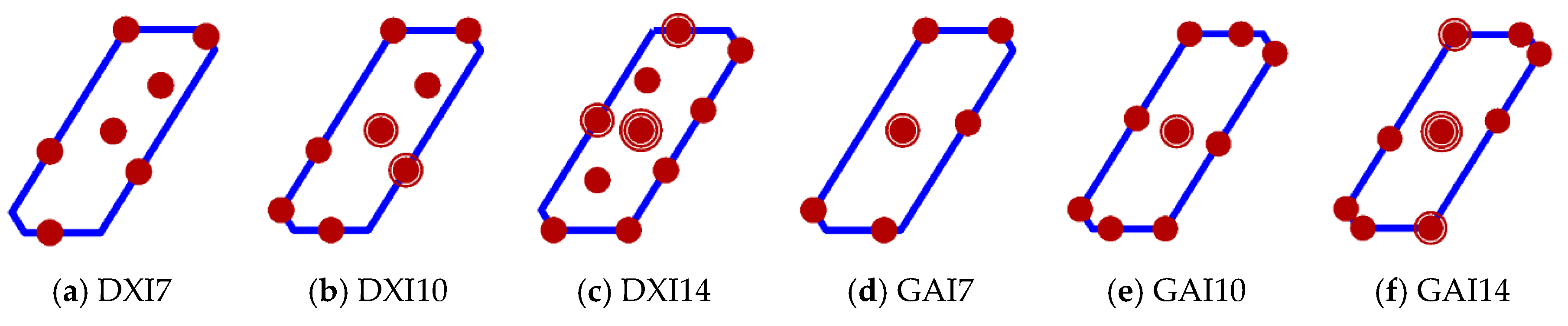
The mixtures from the GA and DX designs in the constrained SCC mixture space are shown in Figure 1. The patterns of points are quite different. The majority of points in the GA designs are distributed around the boundary with replications near the overall centroid, while the DX designs also tend to place design points on the boundary but at different locations and the number of replicates differ from the GA designs. Additionally, the DX designs select multiple mixtures as interior points, while the interior points of the GA designs are concentrated with replicates at only one mixture. The fact that the mixtures selected differ between DX and GA designs is based on the fact the DX designs were constructed only to optimize with respect to one model (the quadratic mixture model), while the GA design considered eight potential models when optimizing. Additionally, DX designs were generated using exchange algorithms that restrict mixture selection from only a finite candidate set of mixtures, while GA designs explore the continuum of points in the entire mixture space.

The next comparison is summarized in

Table 6. The D-, A-, G-, and IV-efficiency.

$\mathit{N}$	Design	D-Efficiency	A-Efficiency	G-Efficiency	IV-Efficiency
7	DX7	0.2329	0.0036	32.4052	0.2152
	GA7	0.2729	0.0038	57.1217	0.2503
10	DX10	0.2443	0.0045	37.2507	0.2291
	GA10	0.2989	0.0057	75.7591	0.2642
14	DX14	0.2284	0.0039	36.0426	0.2226
	GA14	0.2900	0.0047	68.8525	0.2592

, which contains D-, A-, G- and IV-efficiencies for the six designs. Based on the D-, A, G-, and IV-efficiency, the GA designs are superior to the DX designs. What is interesting about these results is that, even though Design-Expert generated designs with the goal of optimizing the IV-efficiency for the quadratic mixture model, the GA design was more IV-efficient (despite weighting over eight models) for the quadratic model.

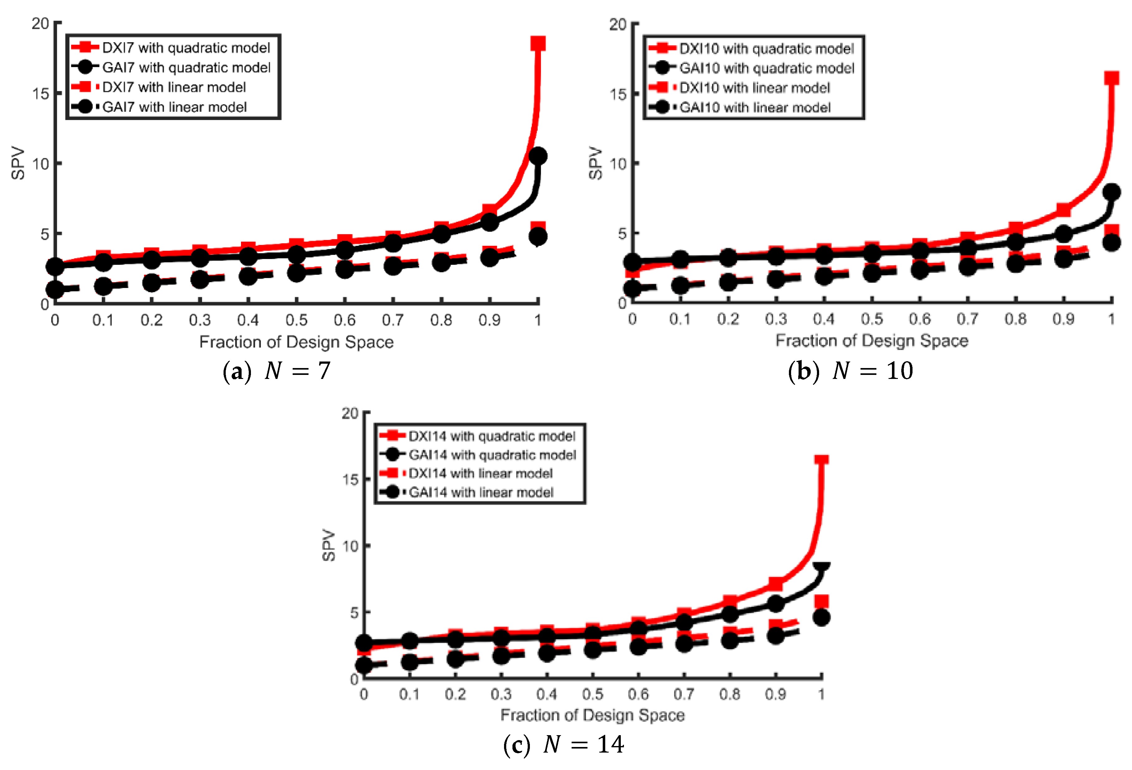
The final comparison uses fraction-of-design-space (FDS) plots to examine model robustness. A model-robust design should perform consistently well with respect to the scaled predictions in the design region for all possible reduced models. The vertical axis represents possible scaled prediction variance $v\left({\mathit{x}}_{\mathbf{0}}\right)$ values (Equation (5)) and the horizontal axis represents the fraction of the mixture design space that has scaled prediction variance values less than or equal to $v\left({\mathit{x}}_{\mathbf{0}}\right)$. Thus, a FDS plot is equivalent to a cumulative distribution function plot but with the axes reversed. For additional information of the FDS plots for examining model robustness, see Ozol-Godfrey et al. [30].

Although an FDS plot can be made for each model, we restrict the study to the quadratic (full) mixture model and the most parsimonious linear mixture model because these curves give a manageable summary of that design’s prediction variance performance at the extremes in terms of model parameters. These FDS plots are presented in Figure 2.

For the linear mixture model, the GA and the DX designs have similar scaled prediction variance distributions for most of the design space. However, for the quadratic mixture model, the DX designs performs poorly for most of the design space compared to the GA designs. This provides evidence for why the IV-efficiencies are smaller for the GA designs compared to the DX designs. For most of the design space, the GA designs appear to have good robustness properties because it has much flatter and lower FDS curves for both the quadratic and linear mixture models, indicating more desirable prediction variance distributions.

5. Conclusions

In this paper, we introduced the concept of a weighted IV-efficiency, which was then used as the objective function of a GA when generating IV-efficient designs robust to a set of reduced models. The goal of the weighted IV-optimality criterion is to find a set of points that will minimize the weighted average of the average of the scaled prediction variance over the design region across a set of reduced models. The IV-efficiencies are calculated over a set of points randomly selected in the experimental region rather than a fixed set of points to get unbiased estimates of weighted IV-efficiencies. Additional assumptions—(i) that not all models should be weighted equally and (ii) that only models having an equal number of model parameters receive equal weight—were adopted for calculating the weighted IV-efficiency.

We studied the problem of generating weighted IV-optimal designs for mixture experiments where the experimental region in an irregularly shaped polyhedron is formed by single component constraints. The proposed methodology allows movement through a continuous region that includes highly constrained mixture regions and does not require selecting points from a user-defined candidate set of mixtures unlike traditional exchange algorithm approaches.

The GA presented in this research paper is effective for generating model-robust designs. The results from the example show that GA designs performed better than the Design Expert designs when examining the model robustness using FDS plots, as well as the D-, A-, G- and IV-efficiencies. When the experimenter believes that the initial model may not turn out to be the model adopted in the final analysis of the experimental data, GA designs based on weighted IV-efficiency are suggested because they protect against the possibility of having a final model with poor prediction variance properties.

Future research will look for alternatives to using random points to estimate the integrals in the definition of the IV-criterion, additional full and reduced model situations, and alternative schemes for weighting these models when calculating IV-efficiency.

References

- Cornell, J.A. Experiments with Mixtures: Designs, Models, and the Analysis of Mixture Data, 3rd ed.; John Wiley & Sons, Inc.: New York, NY, USA, 2002. [Google Scholar]
- Smith, W.F. Experimental Design for Formulation; The American Statistical Association and the Society for Industrial and Applied Mathematics: Philadelphia, PA, USA, 2005. [Google Scholar]
- McLean, R.A.; Anderson, V.L. Extreme vertices designs of mixture experiments. Technometrics 1966, 8, 447–456. [Google Scholar] [CrossRef]
- Welch, W.J. ACED: Algorithm for the construction of experimental designs. Am. Stat. 1985, 39, 146–148. [Google Scholar] [CrossRef]
- Snee, R.D.; Marquardt, D.W. Extreme vertices designs for linear mixture model. Technometrics 1974, 16, 399–408. [Google Scholar] [CrossRef]
- Snee, R.D. Experiment design for mixture systems with multicomponent constraints. Commun. Stat. Theory Methods 1979, 17, 149–159. [Google Scholar]
- Fedorov, V.V. Theory of Optimal Experiments; Academic Press: New York, NY, USA, 1972. [Google Scholar]
- Mitchell, T.J. An algorithm for the construction of D-optimal experimental designs. Technometrics 1974, 16, 203–210. [Google Scholar]
- Huizenga, H.M.; Heslenfeld, D.J.; Molenaar, P.C.M. Optimal measurement conditions for spatiotemporal EEG/MEG source analysis. Psychometrika 2002, 67, 299–313. [Google Scholar] [CrossRef]
- Smucker, B.J.; Del Castillo, E.; Rosenberger, J.L. Exchange Algorithms for Constructing Model-Robust Experimental Designs. J. Qual. Technol. 2011, 43, 1–15. [Google Scholar] [CrossRef]
- Borkowski, J.J. Using Genetic Algorithm to Generate Small Exact Response Surface Designs. J. Probab. Stat. Sci. 2003, 1, 65–88. [Google Scholar]
- Heredia-Langner, A.; Carlyle, W.M.; Montgomery, D.C.; Borror, C.M.; Runger, G.C. Genetic algorithms for the construction of D-optimal designs. J. Qual. Technol. 2003, 35, 28–46. [Google Scholar] [CrossRef]
- Heredia-Langner, A.; Montgomery, D.C.; Carlyle, W.M.; Borror, C.M. Model-robust optimal designs: A genetic algorithm approach. J. Qual. Technol. 2004, 3, 263–279. [Google Scholar] [CrossRef]
- Juang, Y.; Lin, S.; Kao, H. An adaptive scheduling system with genetic algorithms for arranging employee training programs. Expert Syst. Appl. 2007, 33, 642–651. [Google Scholar] [CrossRef]
- Park, Y.; Montgomery, D.C.; Fowler, J.W.; Borror, C.M. Cost-constrained G-efficient response surface designs for cuboidal regions. Qual. Reliab. Eng. Int. 2006, 22, 121–139. [Google Scholar] [CrossRef]
- Limmun, W.; Borkowski, J.J.; Chomtee, B. Using a Genetic Algorithm to Generate D-optimal Designs for Mixture Experiments. Qual. Reliab. Eng. Int. 2013, 29, 1055–1068. [Google Scholar] [CrossRef]
- Myers, R.H.; Montgomery, D.C.; Anderson-Cook, C. Response Surface Methodology: Process and Product Optimization Using Designed Experiments, 3rd ed.; John Wiley & Sons Inc.: New York, NY, USA, 2009. [Google Scholar]
- Atkinson, A.C.; Donev, A.N.; Tobias, R.D. Optimal Experimental Design, with SAS; Oxford University Press: Oxford, UK, 2007. [Google Scholar]
- Hardin, R.H.; Sloane, N.J.A. A new approach to construction of optimal designs. J. Stat. Plan. Inference 1993, 37, 339–369. [Google Scholar] [CrossRef]
- Syafitri, U.; Sartono, B.; Goos, P. I-optimal design of mixture experiments in the presence of ingredient availability constraints. J. Qual. Technol. 2015, 47, 220–234. [Google Scholar] [CrossRef]
- Borkowski, J.J. A comparison of Prediction Variance Criteria for Response Surface Designs. J. Qual. Technol. 2003, 35, 70–77. [Google Scholar] [CrossRef]
- Coetzer, R.; Haines, L.M. The construction of D- and I-optimal designs for mixture experiments with linear constraints on the components. Chemom. Intell. Lab. Syst. 2017, 171, 112–124. [Google Scholar] [CrossRef]
- Box, G.E.P.; Draper, N.R. A basis for the selection of a response surface design. J. Am. Stat. Assoc. 1959, 54, 622–654. [Google Scholar] [CrossRef]
- Goldberg, D.E. Genetic Algorithms in Search, Optimization and Machine Learning; Addison-Wesley: New York, NY, USA, 1989. [Google Scholar]
- Bäck, T.; Hammel, U.; Schwefel, H.P. Evolutionary computation: Comments on the history and current state. IEEE Trans. Evol. Comput. 1997, 1, 3–17. [Google Scholar] [CrossRef]
- Michalewicz, Z. Genetic Algorithms + Data Structures = Evolution Programs; Springer-Verlag: New York, NY, USA, 1996. [Google Scholar]
- Haupt, R.L.; Haupt, S.E. Practical Genetic Algorithms; John Wiley & Sons, Inc.: Hoboken, NJ, USA, 2004. [Google Scholar]
- Borkowski, J.J.; Piepel, G.F. Uniform designs for highly constrained mixture experiments. J. Qual. Technol. 2009, 41, 1–13. [Google Scholar] [CrossRef]
- Crosier, R.D. Symmetry in mixture experiments. Commun. Stat.-Theory Methods 1991, 20, 1911–1935. [Google Scholar] [CrossRef]
- Ozol-Godfrey, A.; Anderson-Cook, C.M.; Montgomery, D.C. Fraction of design space plots for examining model robustness. J. Qual. Technol. 2005, 37, 223–235. [Google Scholar] [CrossRef]
Figure 1.
The genetic algorithm (GA) designs and Design-Expert (DX) designs.
Figure 2.
The fraction-of-design-space (FDS) plots for all competing designs.