Quantum Control in Qutrit Systems Using Hybrid Rabi-STIRAP Pulses


 and
and 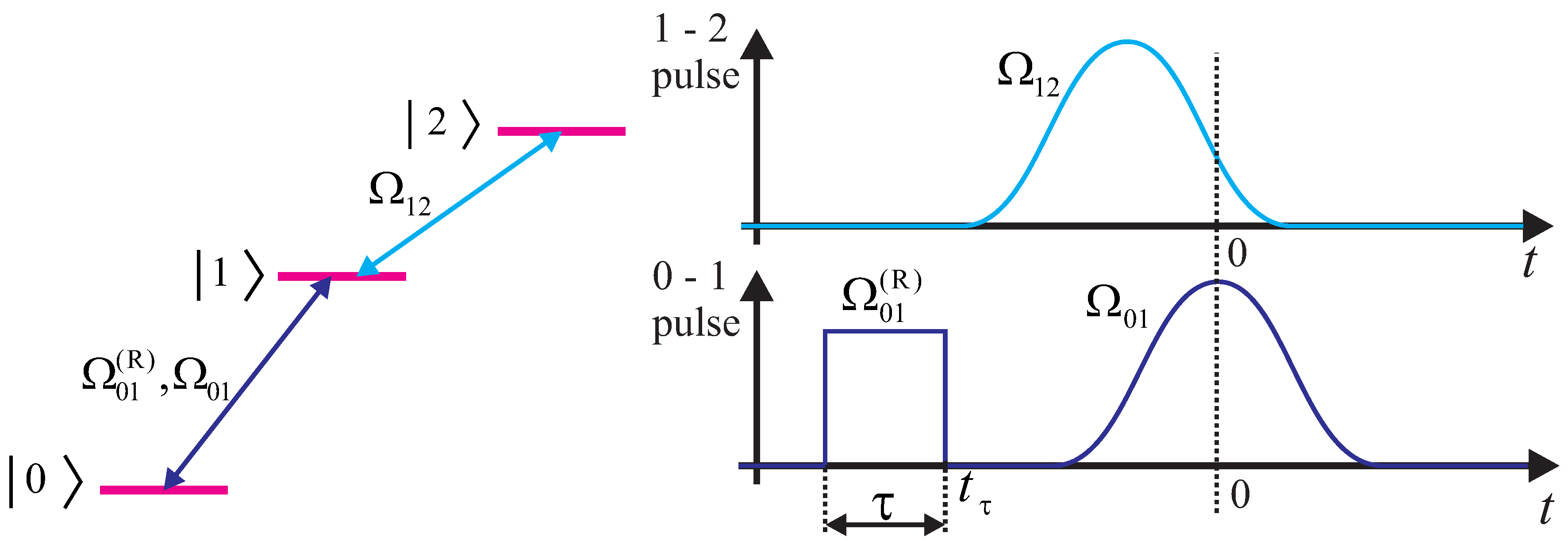
Abstract
:1. Introduction
2. Hybrid Quantum Control in Qutrits
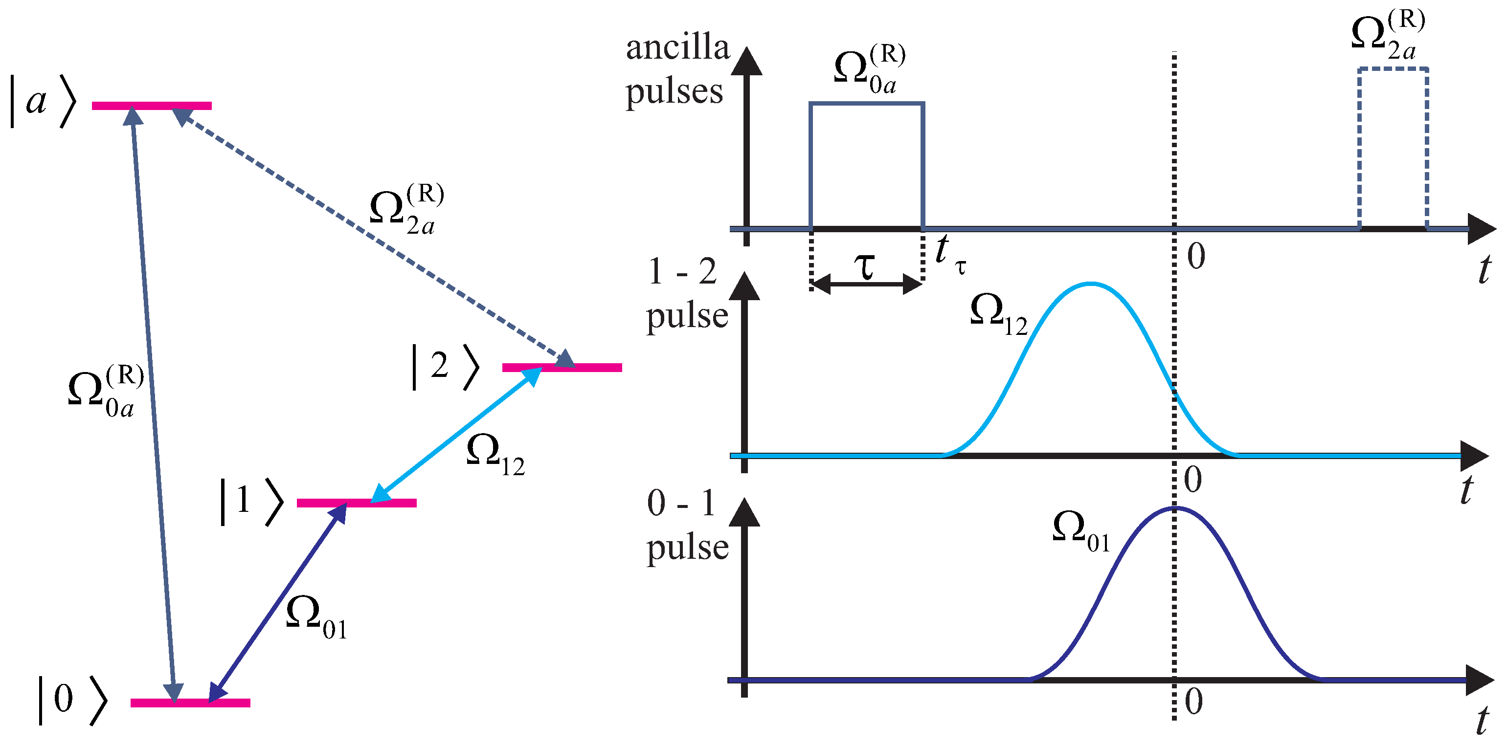
3. Hybrid Pulse Sequence for a Three-Level System with Additional Ancillary State
4. Experimental Implementation in Circuit QED
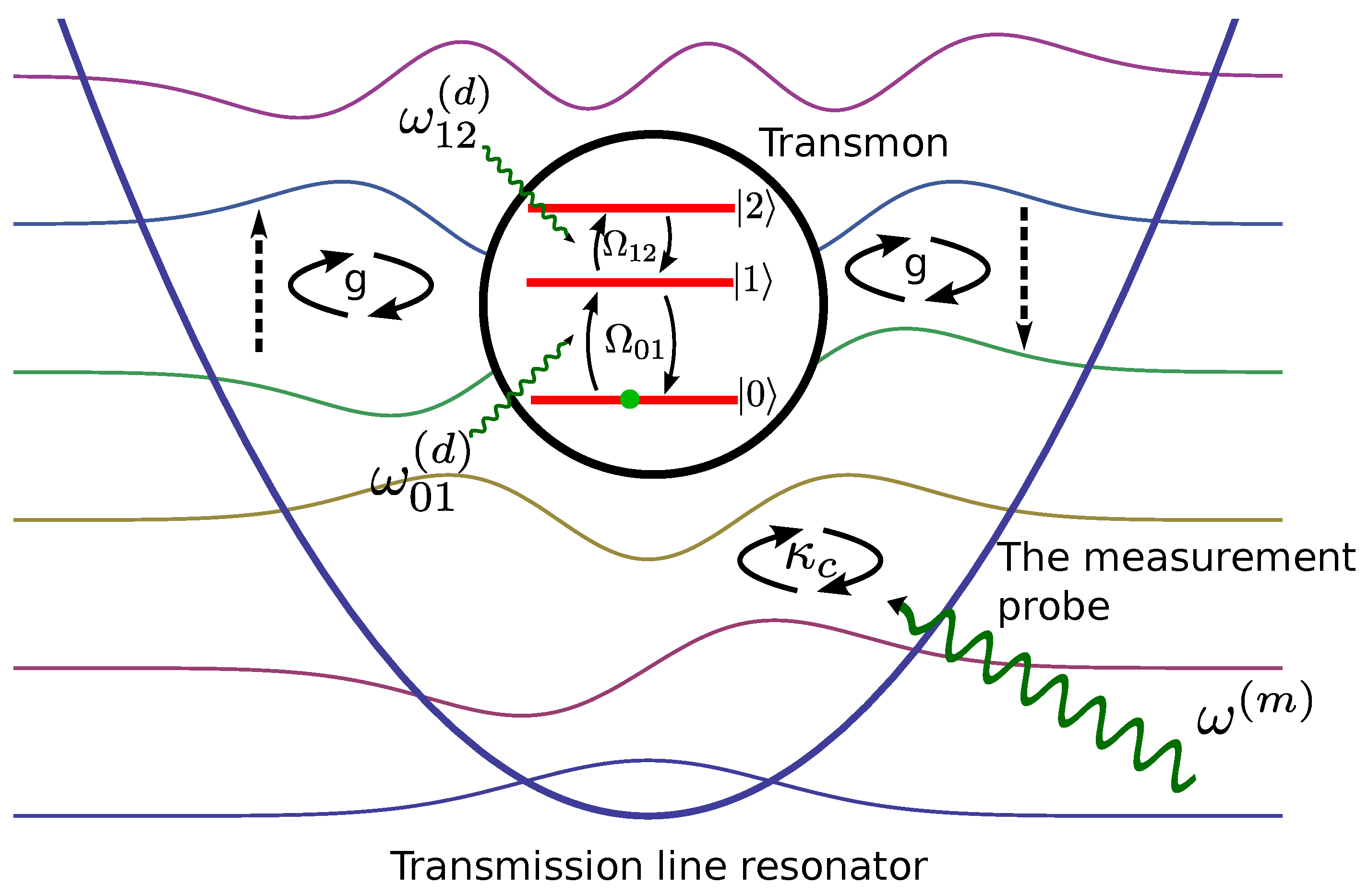
4.1. Superconducting Circuits Realizing Qutrits
4.2. Effective Hamiltonian in a Circuit QED Setup
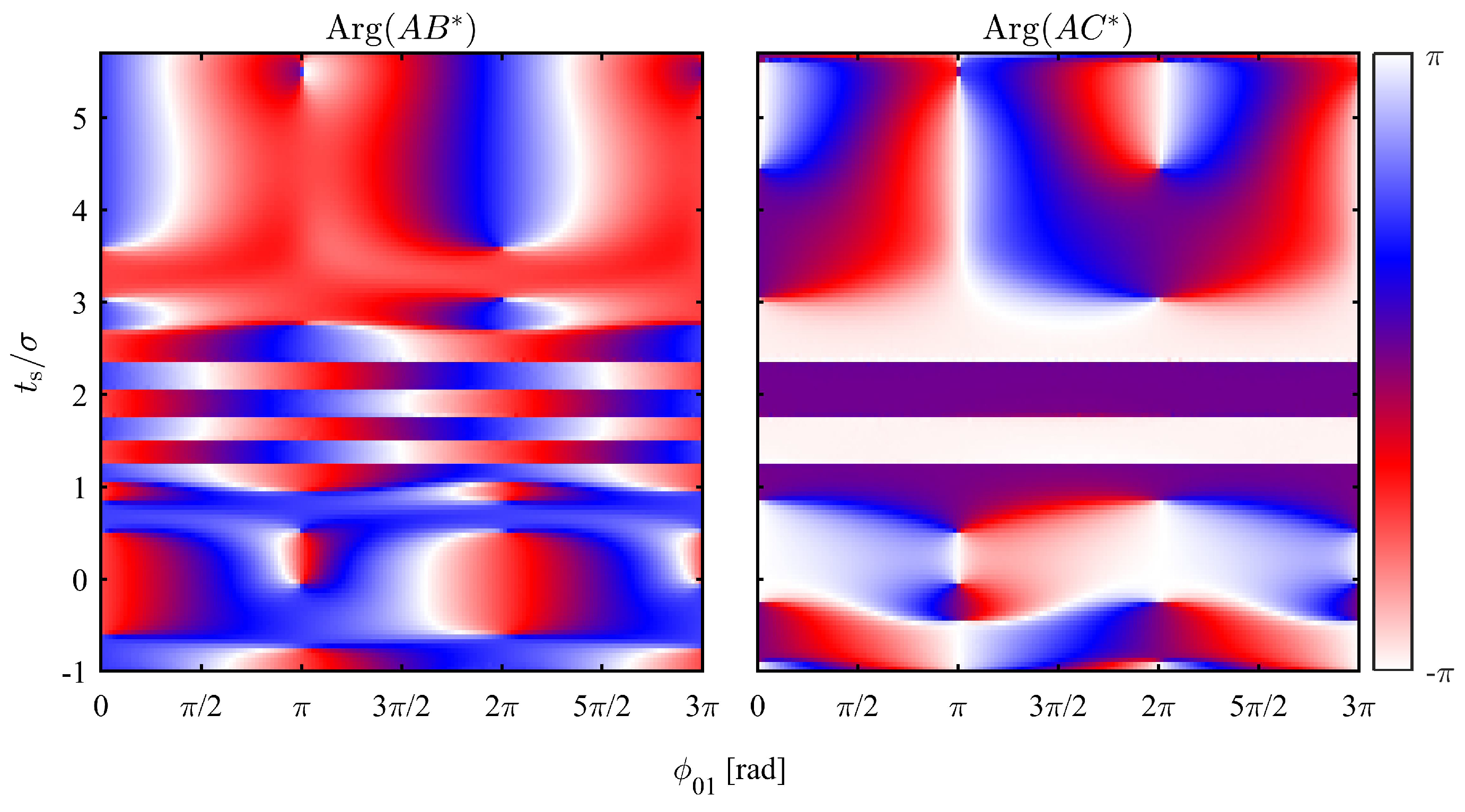
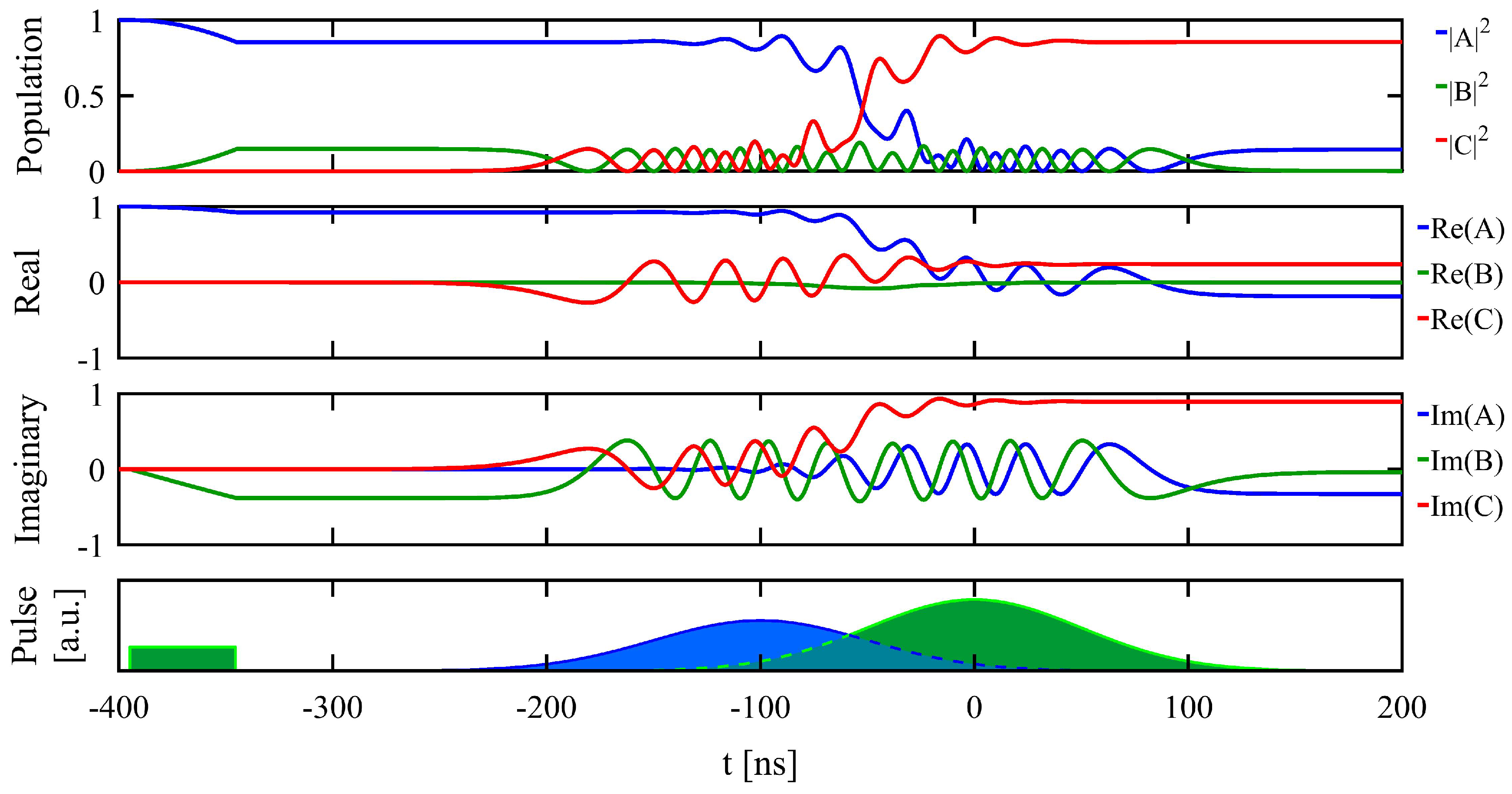
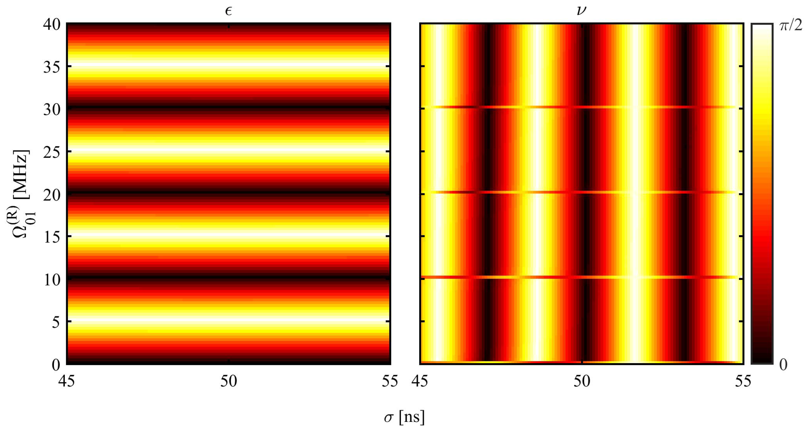
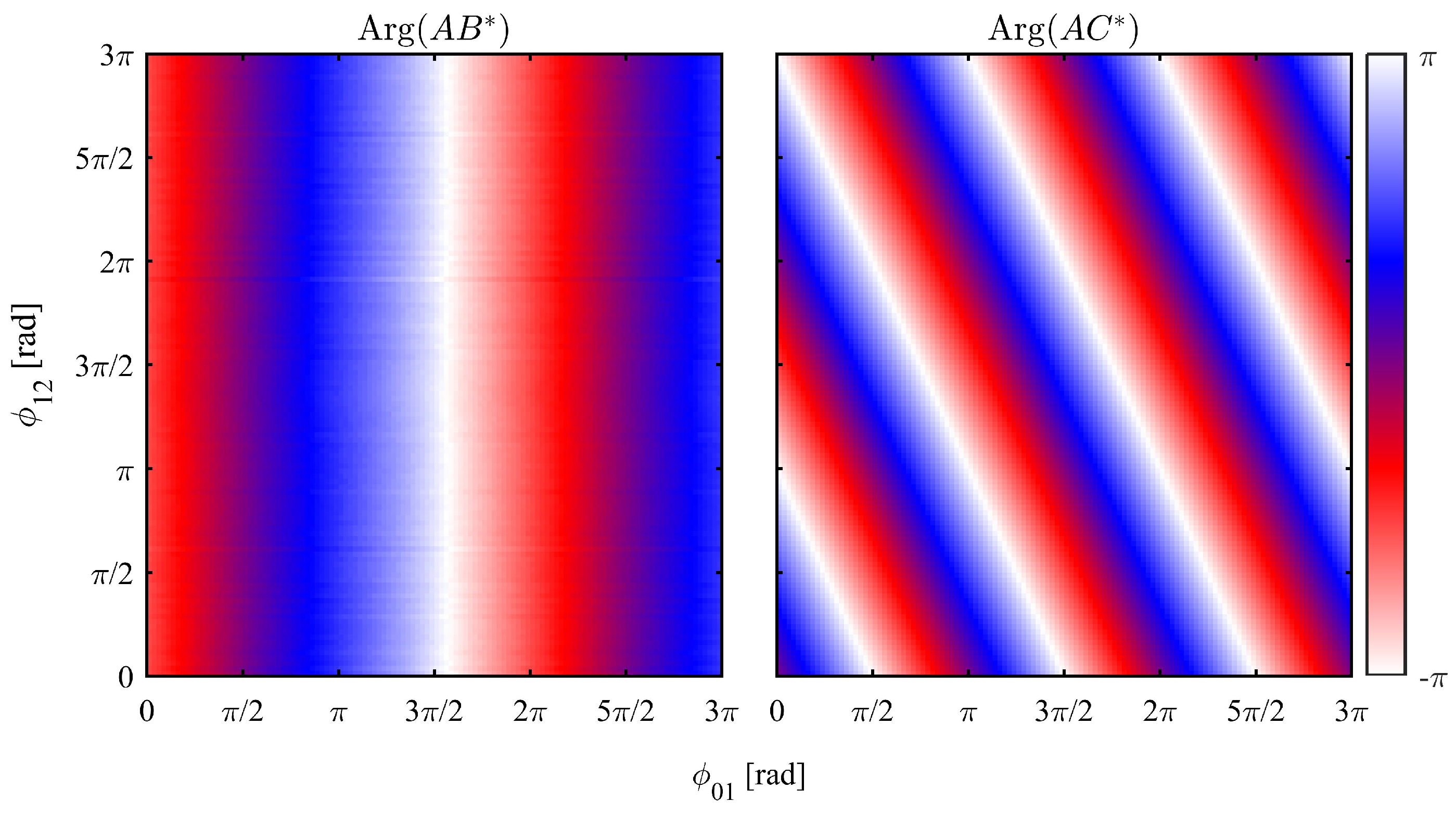
4.3. Hybrid Pulses under Realistic Experimental Conditions
5. Conclusions
Acknowledgments
Author Contributions
Conflicts of Interest
Abbreviations
| STIRAP | stimulated Raman adiabatic passage |
| QED | quantum electrodynamics |
Appendix A. General Three-Level Superposition as Initial State for STIRAP
References
- Ralph, T.C.; Resch, K.; Gilchrist, A. Efficient Toffoli gates using qudits. Phys. Rev. A 2007, 75, 022313. [Google Scholar] [CrossRef]
- Lanyon, B.P.; Barbieri, M.; Almeida, M.P.; Jennewein, T.; Ralph, T.C.; Resch, K.J.; Pryde, G.J.; O’Brien, J.L.; Gilchrist, A.; White, A.G. Simplifying quantum logic using higher-dimensional Hilbert spaces. Nat. Phys. 2009, 5, 134–140. [Google Scholar] [CrossRef]
- Luo, M.X.; Ma, S.Y.; Chen, X.B.; Yang, Y.X. The Power of Qutrit Logic for Quantum Computation. Int. J. Theor. Phys. 2013, 52, 2959–2965. [Google Scholar] [CrossRef]
- Bergmann, K.; Theuer, H.; Shore, B.W. Coherent population transfer among quantum states of atoms and molecules. Rev. Mod. Phys. 1998, 70, 1003–1025. [Google Scholar] [CrossRef]
- Vitanov, N.V.; Halfmann, T.; Shore, B.W.; Bergmann, K. Laser-induced population transfer by adiabatic passage techniques. Annu. Rev. Phys. Chem. 2001, 52, 763–809. [Google Scholar] [CrossRef] [PubMed]
- Baur, M.; Filipp, S.; Bianchetti, R.; Fink, J.M.; Göppl, M.; Steffen, L.; Leek, P.J.; Blais, A.; Wallraff, A. Measurement of Autler-Townes and Mollow Transitions in a Strongly Driven Superconducting Qubit. Phys. Rev. Lett. 2009, 102, 243602. [Google Scholar] [CrossRef] [PubMed]
- Kelly, W.R.; Dutton, Z.; Schlafer, J.; Mookerji, B.; Ohki, T.A.; Kline, J.S.; Pappas, D.P. Direct Observation of Coherent Population Trapping in a Superconducting Artificial Atom. Phys. Rev. Lett. 2010, 104, 163601. [Google Scholar] [CrossRef] [PubMed]
- Abdumalikov, A.A.; Astafiev, O.; Zagoskin, A.M.; Pashkin, Y.A.; Nakamura, Y.; Tsai, J.S. Electromagnetically Induced Transparency on a Single Artificial Atom. Phys. Rev. Lett. 2010, 104, 193601. [Google Scholar] [CrossRef] [PubMed]
- Sillanpää, M.A.; Li, J.; Cicak, K.; Altomare, F.; Park, J.I.; Simmonds, R.W.; Paraoanu, G.S.; Hakonen, P.J. Autler-Townes Effect in a Superconducting Three-Level System. Phys. Rev. Lett. 2009, 103, 193601. [Google Scholar] [CrossRef] [PubMed]
- Li, J.; Paraoanu, G.S.; Cicak, K.; Altomare, F.; Park, J.I.; Simmonds, R.W.; Sillanpää, M.A.; Hakonen, P.J. Decoherence, Autler-Townes effect, and dark states in two-tone driving of a three-level superconducting system. Phys. Rev. B 2011, 84, 104527. [Google Scholar] [CrossRef]
- Li, J.; Paraoanu, G.S.; Cicak, K.; Altomare, F.; Park, J.I.; Simmonds, R.W.; Sillanpää, M.A.; Hakonen, P.J. Dynamical Autler-Townes control of a phase qubit. Sci. Rep. 2012, 2, 645. [Google Scholar] [CrossRef] [PubMed]
- Peterer, M.J.; Bader, S.J.; Jin, X.; Yan, F.; Kamal, A.; Gudmundsen, T.J.; Leek, P.J.; Orlando, T.P.; Oliver, W.D.; Gustavsson, S. Coherence and Decay of Higher Energy Levels of a Superconducting Transmon Qubit. Phys. Rev. Lett. 2015, 114, 010501. [Google Scholar] [CrossRef] [PubMed]
- Jerger, M.; Reshitnyk, Y.; Oppliger, M.; Potoćnik, A.; Mondal, M.; Wallraff, A.; Goodenough, K.; Wehner, S.; Juliusson, K.; Langford, N.K.; et al. Contextuality without nonlocality in a superconducting quantum system. Nat. Commun. 2016, 7, 12930. [Google Scholar] [CrossRef] [PubMed]
- You, J.Q.; Nori, F. Atomic physics and quantum optics using superconducting circuits. Nature 2011, 474, 589–597. [Google Scholar] [CrossRef] [PubMed]
- Falci, G.; Stefano, P.G.D.; Ridolfo, A.; D’Arrigo, A.; Paraoanu, G.S.; Paladino, E. Advances in quantum control of three-level superconducting circuit architectures. Fortschr. Phys. 2016, 1–10. [Google Scholar] [CrossRef]
- Siewert, J.; Brandes, T.; Falci, G. Advanced control with a Cooper-pair box: Stimulated Raman adiabatic passage and Fock-state generation in a nanomechanical resonator. Phys. Rev. B 2009, 79, 024504. [Google Scholar] [CrossRef]
- Falci, G.; La Cognata, A.; Berritta, M.; D’Arrigo, A.; Paladino, E.; Spagnolo, B. Design of a Lambda system for population transfer in superconducting nanocircuits. Phys. Rev. B 2013, 87, 214515. [Google Scholar] [CrossRef]
- Di Stefano, P.G.; Paladino, E.; Pope, T.J.; Falci, G. Coherent manipulation of noise-protected superconducting artificial atoms in the Lambda scheme. Phys. Rev. A 2016, 93, 051801. [Google Scholar] [CrossRef]
- Koch, J.; Yu, T.M.; Gambetta, J.; Houck, A.A.; Schuster, D.I.; Majer, J.; Blais, A.; Devoret, M.H.; Girvin, S.M.; Schoelkopf, R.J. Charge insensitive qubit design derived from the Cooper pair box. Phys. Rev. A 2007, 76, 042319. [Google Scholar] [CrossRef]
- Kumar, K.S.; Vepsäläinen, A.; Danilin, S.; Paraoanu, G.S. Stimulated Raman adiabatic passage in a three-level superconducting circuit. Nat. Commun. 2016, 7, 10628. [Google Scholar] [CrossRef] [PubMed]
- Paraoanu, G.S. Recent progress in quantum simulation using superconducting circuits. J. Low Temp. Phys. 2014, 175, 633–654. [Google Scholar] [CrossRef]
- Neeley, M.; Ansmann, M.; Bialczak, R.C.; Hofheinz, M.; Lucero, E.; O’Connell, A.D.; Sank, D.; Wang, H.; Wenner, J.; Cleland, A.N.; et al. Emulation of a Quantum Spin with a Superconducting Phase Qudit. Science 2009, 325, 722–725. [Google Scholar] [CrossRef] [PubMed]
- Malinovsky, V.S.; Tannor, D.J. Simple and robust extension of the stimulated Raman adiabatic passage technique to N-level systems. Phys. Rev. A 1997, 56, 4929–4937. [Google Scholar] [CrossRef]
- Unanyan, R.; Fleischhauer, M.; Shore, B.; Bergmann, K. Robust creation and phase-sensitive probing of superposition states via stimulated Raman adiabatic passage (STIRAP) with degenerate dark states. Opt. Commun. 1998, 155, 144–154. [Google Scholar] [CrossRef]
- Unanyan, R.G.; Shore, B.W.; Bergmann, K. Preparation of an N-component maximal coherent superposition state using the stimulated Raman adiabatic passage method. Phys. Rev. A 2001, 63, 043401. [Google Scholar] [CrossRef]
- Karpati, A.; Kis, Z. Adiabatic creation of coherent superposition states via multiple intermediate states. J. Phys. B At. Mol. Opt. Phys. 2003, 36, 905–919. [Google Scholar] [CrossRef]
- Vitanov, N.; Fleischhauer, M.; Shore, B.; Bergmann, K. Coherent Manipulation of Atoms Molecules by Sequential Laser Pulses. Adv. At. Mol. Opt. Phys. 2001, 46, 55–190. [Google Scholar]
- Vitanov, N.V.; Halfmann, T.; Shore, B.W.; Bergmann, K. Laser-induced population transfer by adiabatic passage techniques. Annu. Rev. Phys. Chem. 2001, 52, 763–809. [Google Scholar] [CrossRef] [PubMed]
- Møller, D.; Madsen, L.B.; Mølmer, K. Geometric phase gates based on stimulated Raman adiabatic passage in tripod systems. Phys. Rev. A 2007, 75, 062302. [Google Scholar] [CrossRef]
- Leek, P.; Fink, J.M.; Blais, A.; Bianchetti, R.; Göppl, M.; Gambetta, J.; Schuster, D.; Frunzio, L.; Schoelkopf, R.; Wallraff, A. Observation of Berry’s Phase in a Solid State Qubit. Science 2007, 318, 1889–1892. [Google Scholar] [CrossRef] [PubMed]
- Abdumalikov, A.A.; Fink, J.M.; Juliusson, K.; Pechal, M.; Berger, S.; Wallraff, A.; Filipp, S. Experimental Realization of Non-Abelian Geometric Gates. Nature 2013, 496, 482–485. [Google Scholar] [CrossRef] [PubMed]
- Josephson, B.D. Possible new effects in superconductive tunnelling. Phys. Lett. 1962, 1, 251–253. [Google Scholar] [CrossRef]
- Backhaus, S.; Pereverzev, S.V.; Loshak, A.; Davis, J.C.; Packard, R.E. Direct Measurement of the Current-Phase Relation of a Superfluid 3He-B Weak Link. Science 1997, 278, 1435–1438. [Google Scholar] [CrossRef] [PubMed]
- Sukhatme, K.; Mukharsky, Y.; Chui, T.; Pearson, D. Observation of the ideal Josephson effect in superfluid 4He. Nature 2001, 411, 280–283. [Google Scholar] [CrossRef] [PubMed]
- Leggett, A.J. Bose-Einstein condensation in the alkali gases: Some fundamental concepts. Rev. Mod. Phys. 2001, 73, 307–356. [Google Scholar] [CrossRef]
- Paraoanu, G.S.; Rodriguez, M.; Törmä, P. Josephson effect in superfluid atomic Fermi gases. Phys. Rev. A 2002, 66, 041603. [Google Scholar] [CrossRef]
- Heikkinen, M.O.J.; Massel, F.; Kajala, J.; Leskinen, M.J.; Paraoanu, G.S.; Törmä, P. Spin-Asymmetric Josephson Effect. Phys. Rev. Lett. 2010, 105, 225301. [Google Scholar] [CrossRef] [PubMed]
- Pekola, J.P.; Hirvi, K.P.; Kauppinen, J.P.; Paalanen, M.A. Thermometry by Arrays of Tunnel Junctions. Phys. Rev. Lett. 1994, 73, 2903–2906. [Google Scholar] [CrossRef] [PubMed]
- Meschke, M.; Kemppinen, A.; Pekola, J. Accurate Coulomb Blockade Thermometry up to 60 Kelvin. Philos. Trans. R. Soc. A 2016, 374, 20150052. [Google Scholar] [CrossRef] [PubMed]
- Kastner, M.A. The single-electron transistor. Rev. Mod. Phys. 1992, 64, 849–858. [Google Scholar] [CrossRef]
- Schoelkopf, R.J.; Wahlgren, P.; Kozhevnikov, A.A.; Delsing, P.; Prober, D.E. The Radio-Frequency Single-Electron Transistor (RF-SET): A Fast and Ultrasensitive Electrometer. Science 1998, 280, 1238–1242. [Google Scholar] [CrossRef] [PubMed]
- Paraoanu, G.S.; Halvari, A.M. Suspended single-electron transistors: Fabrication and measurement. Appl. Phys. Lett. 2005, 86, 093101. [Google Scholar] [CrossRef]
- Feshchenko, A.V.; Koski, J.V.; Pekola, J.P. Experimental realization of a Coulomb blockade refrigerator. Phys. Rev. B 2014, 90, 201407. [Google Scholar] [CrossRef]
- Toppari, J.J.; Kühn, T.; Halvari, A.P.; Kinnunen, J.; Leskinen, M.; Paraoanu, G.S. Cooper-pair resonances and subgap Coulomb blockade in a superconducting single-electron transistor. Phys. Rev. B 2007, 76, 172505. [Google Scholar] [CrossRef]
- Koski, J.V.; Kutvonen, A.; Khaymovich, I.M.; Ala-Nissila, T.; Pekola, J.P. On-Chip Maxwell’s Demon as an Information-Powered Refrigerator. Phys. Rev. Lett. 2015, 115, 260602. [Google Scholar] [CrossRef] [PubMed]
- Fulton, T.A.; Gammel, P.L.; Bishop, D.J.; Dunkleberger, L.N.; Dolan, G.J. Observation of combined Josephson and charging effects in small tunnel junction circuits. Phys. Rev. Lett. 1989, 63, 1307–1310. [Google Scholar] [CrossRef] [PubMed]
- Haviland, D.B.; Harada, Y.; Delsing, P.; Chen, C.D.; Claeson, T. Observation of the Resonant Tunneling of Cooper Pairs. Phys. Rev. Lett. 1994, 73, 1541–1544. [Google Scholar] [CrossRef] [PubMed]
- Risté, D.; Bultink, C.C.; Tiggelman, M.J.; Schouten, R.N.; Lehnert, K.W.; DiCarlo, L. Millisecond charge-parity fluctuations and induced decoherence in a superconducting transmon qubit. Nat. Commun. 2013, 4, 1913. [Google Scholar] [CrossRef] [PubMed]
- Schuster, D.I.; Wallraff, A.; Blais, A.; Frunzio, L.; Huang, R.S.; Majer, J.; Girvin, S.M.; Schoelkopf, R.J. ac Stark Shift and Dephasing of a Superconducting Qubit Strongly Coupled to a Cavity Field. Phys. Rev. Lett. 2005, 94, 123602. [Google Scholar] [CrossRef] [PubMed]


© 2016 by the authors; licensee MDPI, Basel, Switzerland. This article is an open access article distributed under the terms and conditions of the Creative Commons Attribution (CC-BY) license (http://creativecommons.org/licenses/by/4.0/).
Share and Cite
Vepsäläinen, A.; Danilin, S.; Paladino, E.; Falci, G.; Paraoanu, G.S. Quantum Control in Qutrit Systems Using Hybrid Rabi-STIRAP Pulses. Photonics 2016, 3, 62. https://doi.org/10.3390/photonics3040062
Vepsäläinen A, Danilin S, Paladino E, Falci G, Paraoanu GS. Quantum Control in Qutrit Systems Using Hybrid Rabi-STIRAP Pulses. Photonics. 2016; 3(4):62. https://doi.org/10.3390/photonics3040062
Chicago/Turabian StyleVepsäläinen, Antti, Sergey Danilin, Elisabetta Paladino, Giuseppe Falci, and Gheorghe Sorin Paraoanu. 2016. "Quantum Control in Qutrit Systems Using Hybrid Rabi-STIRAP Pulses" Photonics 3, no. 4: 62. https://doi.org/10.3390/photonics3040062