Novel Equalization Techniques for Space Division Multiplexing Based on Stokes Space Update Rule

Abstract

Space division multiplexing (SDM) is a promising technology that aims to overcome the capacity crunch of optical communications. In this paper, we introduce the multiple-input multiple-output (MIMO) Stokes Space Algorithm (SSA) implemented in frequency domain, a novel equalization technique for space division multiplexing (SDM). Although different papers have been published about the SSA and its MIMO implementation, we provide for the first time an analysis of the of the convergence speed and frequency offset of the SSA compared to the least mean square (LMS). SSA algorithm can deal with higher frequency offsets and linewidths than LMS, being suitable for optical communications with higher phase noise. SSA does not need pre-compensation of frequency offset, which can be compensated after equalization without penalties. On the other hand, due to reduced convergence speed, SSA requires longer training sequences than LMS.

1. Introduction

The achievable data transmission capacity over optical fiber has been growing continuously at exponential rate during the last 30 years. One of the main enablers for this capacity increase is the development of coherent detection, which efficiently maps the full optical field into the electrical domain, presents better sensitivity than direct detection, and allows to overcome signal impairments by means of digital signal processing (DSP) [1]. DSP also relaxes the receiver specifications in favor of equalization, allowing the use of polarization division multiplexing (PDM) without a tight control of the state of polarization of light [2].

On the other hand, the improvement of physical components, such as optical fibers with lower signal impairments and attenuation, allows longer transmission distances while lowering the DSP requirements. In addition, the development of advanced Erbium-Doped Fiber Amplifiers (EDFAs) providing lower noise figures (NF) and wider amplification ranges, enables the allocation of more optical channels on larger optical spectrums by means of dense wavelength-division multiplexing (DWDM), efficiently increases the transmitted throughput on the optical fiber.

By the exploitation of high spectral efficient coding [3], we are finally approaching the fundamental capacity limit of the standard single mode fiber (SSMF) [4,5], where each research effort to increase capacity results in diminishing marginal returns. This scenario, commonly termed as the capacity crunch of optical communications, drives industry and academia to look for alternatives to overcome this limitation.

From a product point of view, we live in the information era where enormous amount of data is generated, transported, and consumed every day. The optical transport network accounts for most of the responsibility in providing the requested data to the end users. Due to the proliferation of bandwidth demanding services such as video streaming, cloud services, or social networks, optical networks have been experimenting a continuous growth of their traffic. This growth is forecasted to continuously increase due to the mainstream of very high definition screens, virtual reality (VR), advance cloud services, or internet-of-things (IoT), with even higher requirements in terms of bandwidth and latency. Fueled by this demand, operators and telecommunications companies are compelled to increase the provided bandwidth, facing important trade-offs concerning: cost-per-bit, form factor, or power consumption of the optical transponders. If the current capacity demand continues to increase, the commercial telecommunication equipment will finally reach the fundamental physical limitation currently experimented in the telecommunication research.

The research community has shown an increasing interest in Space Division Multiplexing (SDM) as the feasible way to increase capacity. SDM adds the spatial dimension to overcome the fundamental limitation by considering multiple parallel spatial propagation paths. Different SDM variants are currently being investigated. In this paper, we provide a discussion of the different SDM approaches and the main DSP techniques needed for each case. We focus on different equalization methods including novel equalization techniques based on Stokes Space recently introduced in [6,7,8].

The presented algorithms are thoroughly studied and evaluated by simulations. The Stokes algorithm implemented in this paper is insensitive to frequency offsets, which eliminates the need of its pre-compensation, enabling to simplify the future SDM receivers at the expense of increasing the convergence speed.

2. Space Division Multiplexing

SDM has acquired great popularity enabling the transmission of previously unthinkable baudrates. Many experiments have validated the high throughput achievable by SDM. Some remarkable cases are the 2.15 Pb/s transmission over 31 km employing a 22 multi-core single mode fiber [9] or the 57.6 Tb/s over 119 km employing a few-mode fiber (FMF) [10]. Further reading and a thorough review of different SDM transmission records can be found at [11].

Since SDM applies to any communication system transmitting different spatial-optical signals, it encompasses a wide range of categories. We review the different SDM technologies [3], with a clear focus on the complexity of the DSP needed. Depending on the transmission medium, two types of equalizers are considered. A single-mode 2 × 2 equalizer, capable of compensating Chromatic Dispersion (CD), Polarization Modal Dispersion (PMD), and State-of-Polarization (SoP) rotation, which is the conventional coherent receiver for SMF and valid for SDM systems exhibiting low or negligible crosstalk, and a multi-mode 2M × 2M equalizer, where $M$ is the number of modes that are mixing, capable of compensating all the impairments of the single-mode equalizer, and in addition differential modal group delay (DMGD) and mode mixing between the different spatial modes.

The simpler approach to implement SDM is packaging multiple fiber together in fiber-bundles. Since the fibers involved maintain their properties, no crosstalk is expected between the different fibers, requiring parallel single-mode equalizers. A similar approach consists of placing different cores inside the same fiber resulting in multi-core fibers (MCF). As the core spacing may be in the range of the decay of the single cores’ evanescent waves, crosstalk between the different cores may arise [12]. Fiber design of MCF (core number, core spacing, etc.) is critical for minimizing the crosstalk between modes and achieving optimum propagation settings for each scenario [13]. Depending on the fiber parameters and the distance of the link, the accumulated crosstalk may allow signal recovery by means of parallel single-mode equalization for each transmitted mode. Alternatively, if the crosstalk between the modes is high enough, multi-mode MIMO equalization 2M × 2M may be needed.

Another approach is to increase the numerical aperture of the fiber, allowing the propagation of higher order modes inside the same fiber. Depending on the number of supported modes, the respective fibers are multi-mode fiber (MMF) or few-mode fiber (FMF). The transmission over MMF or FMF generally results in mixing between different modes and needs complex DSP for its compensation [14] with multi-mode equalizers.

Mode multiplexing in MMF and FMF is commonly focused on LP modes [3]. Alternatively, another set of orthogonal modes may be excited, like orbital angular momentum (OAM) modes, that exhibit less degeneracy of propagation constant and thus less severe (resonant) crosstalk between the modes. The generation of OAM modes can be done by means of ring resonators or its conversion by free space optics employing Spatial Light Modulators (SLM) [15]. OAM modes also require the design of specific optical fibers that are capable of removing aforementioned degeneracy and thus of suppressing mode coupling such as the inverse-parabolic graded-index fiber (IPGIF) [16]. Even though these fibers can prevent mode coupling in theory, the transmission of OAM modes with tolerable crosstalk is only possible for short distances (in the order of a few km [17]) due to the imperfections of the fiber, fiber coupling, and bending.

Another type of fiber merging previous approaches is the hybrid fiber, which combines few-mode fiber and multicore fiber (FMF-MCF), resulting in higher density of modes and enabling the transmission of multiple modes per core [18]. A variant of MCF is the coupled-core fibers involving a higher granularity of cores in the fiber making dense multi-mode equalization indispensable due to strong crosstalk. Coupled-core fibers can support supermode multiplexing, i.e., the simultaneous propagation of modes in different cores. Supermodes can be arranged in groups transmitting the same signal, over different modes and cores, resulting in similar performance as MMF [19].

3. Equalizers for SDM

Commonly, the coherent detection is divided into three modules: optical front-end, analogue-to-digital converter (ADC), and the DSP module [1]. The optical front-end is responsible for the down-conversion of the optical signal into the electrical domain, which is subsequently converted into the digital domain by the ADC. The DSP module compensates for the signal impairments and obtains the information stream modulated over the signal.

In this paper, we focus on the DSP module, revising the single-mode equalization techniques by reviewing different error functions: least mean square (LMS) and Stokes space algorithm (SSA). We also explain the multi-mode generalization: 2M × 2M, including the novel 2M × 2M SSA-MIMO algorithm.

3.1. Single-Mode 2 × 2 Dynamic Equalization

The 2 × 2 equalization consists of 4 filters compensating for the impulse response of the transmission channel over the input signals (${\mathit{h}}_{xx}^{\left(n\right)}$ and ${\mathit{h}}_{yy}^{\left(n\right)}$) and the respective mixing components (${\mathit{h}}_{xy}^{\left(n\right)}$ and ${\mathit{h}}_{yx}^{\left(n\right)}$):

$$\overline{x}\left(n\right)={\mathit{x}}^{\left(n\right)}·{\mathit{h}}_{xx}^{\left(n\right)}+{\mathit{y}}^{\left(n\right)}·{\mathit{h}}_{xy}^{\left(n\right)};\overline{y}\left(n\right)={\mathit{x}}^{\left(n\right)}·{\mathit{h}}_{yx}^{\left(n\right)}+{\mathit{y}}^{\left(n\right)}·{\mathit{h}}_{yy}^{\left(n\right)},$$

(1)

where the input signals ${\mathit{x}}^{\left(n\right)}$ and ${\mathit{y}}^{\left(n\right)}$ are vectors accounting for $N$ samples of the received signals: ${\mathit{x}}^{\left(n\right)}=\left[x\left(n\right),x\left(n-1\right)\dots x\left(n-N+1\right)\right]$and ${\mathit{y}}^{\left(n\right)}=\left[y\left(n\right),y\left(n-1\right)\dots y\left(n-N+1\right)\right].$ The ‘$·$’ represents the dot product operation, and the filter coefficients are vectors of $N$taps, where the number of taps should be, at least, as long as the impulse response of the system for enabling the compensation of the signal impairments:

$$\begin{gathered} {\mathit{h}}_{xx}^{\left(n\right)}=[h_{xx}^{\left(n\right)}\left(1\right),h_{xx}^{\left(n\right)}\left(2\right)\dots h_{xx}^{\left(n\right)}\left(N\right)];{\mathit{h}}_{xy}^{\left(n\right)}=[h_{xy}^{\left(n\right)}\left(1\right),h_{xy}^{\left(n\right)}\left(2\right)\dots h_{xy}^{\left(n\right)}\left(N\right)], \\ {\mathit{h}}_{yx}^{\left(n\right)}=[h_{yx}^{\left(n\right)}\left(1\right),h_{yx}^{\left(n\right)}\left(2\right)\dots h_{yx}^{\left(n\right)}\left(N\right)];{\mathit{h}}_{yy}^{\left(n\right)}=[h_{yy}^{\left(n\right)}\left(1\right),h_{yy}^{\left(n\right)}\left(2\right)\dots h_{yy}^{\left(n\right)}\left(N\right)]. \end{gathered}$$

(2)

The update algorithms considered in this paper are based on the stochastic gradient update [1], where the equalized signal is compared with the expected transmitted signal by means of the equalizer’s error function [6]. For the error functions considered in this paper, the stochastic gradient update can be expressed as:

$$\begin{gathered} {\mathit{h}}_{lm}^{\left(n+1\right)}={\mathit{h}}_{lm}^{\left(n\right)}-\mu {\nabla }_{{\mathit{h}}_{lm}^{\left(n\right)}}f({\mathit{h}}^{\left(n\right)});l,m\in \left\{x,y\right\}, \\ {\nabla }_{{\mathit{h}}_{lm}^{\left(n\right)}}f({\mathit{h}}^{\left(n\right)})=C_p\left(n\right)m^{*\left(n\right)}, \\ p=\{\begin{array}{c}1,l=x\\ 2,l=y\end{array};\mathit{m}\in \left\{\mathit{x},\mathit{y}\right\}. \end{gathered}$$

(3)

The error function determines how filter coefficients are updated, influencing the performance of the system. The other parameter that might impact on the performance is the step size μ. The step size influences the stability, the convergence speed, and the final performance of the equalizer [20]. The step size should be carefully tuned for each application and equalizer.

The filter update rule given by Equation (3) includes two error coefficients: $C_1$ and $C_2$, being the error coefficients of the $x$ and $y$ polarizations, which are determined by the error function of the equalizer.

3.1.1. Least Mean Square

The LMS equalization is one of the most well-known equalizers based on an approximation of the Wiener-Hopf solution [21]. The LMS error function is computed as the square difference between the equalized signal and the expected one for each polarization:

$$f_{LMS}\left(h\left(n\right)\right)={\left|\overline{x}\left(n\right)-\widehat{x}\left(n\right)\right|}^2+{\left|\overline{y}\left(n\right)-\widehat{y}\left(n\right)\right|}^2,$$

(4)

where $\widehat{x}$ and $\widehat{y}$ are the expected signals. The LMS equalizer can operate in two different ways: training mode and decision-directed (DD) mode. In training mode, transmitter and receiver agree in using a specific signal, called the training sequence, which is known by both. The training sequence is used for enabling the initial pre-convergence of the weights. After the training period, the equalizer switches to DD mode, directly applying decisions over the equalizer data to estimate the transmitted signals.

According to the introduced description of the stochastic gradient descent update rule, the LMS algorithm has the following error coefficients:

$$C_1\left(n\right)=2\left(\overline{x}\left(n\right)-\widehat{x}\left(n\right)\right)\overline{x}\left(n\right);C_2\left(n\right)=2\left(\overline{y}\left(n\right)-\widehat{y}\left(n\right)\right)\overline{y}\left(n\right).$$

(5)

As expected, it is observable that $C_1\left(n\right)$ and $C_2\left(n\right)$ are only functions of x and y polarization respectively.

3.1.2. Stokes Space Algorithm

The Stokes space transformation has been actively used for characterizing signal and its impairments [22]. The Stokes transformation converts the 2-D complex Jones space, $\left\{x,y\right\}\in \Im$, into a 3-D real space: $\{S_1,S_2,S_3\}\in ℝ$:

$$\begin{gathered} S_1\left(n\right)={\left|x\left(n\right)\right|}^2-{\left|y\left(n\right)\right|}^2, \\ {S}_2\left(n\right)=2\Re \left\{x\left(n\right)y^{*}\left(n\right)\right\}, \\ {S}_3\left(n\right)=2\Im \left\{x\left(n\right)y^{*}\left(n\right)\right\}. \end{gathered}$$

(6)

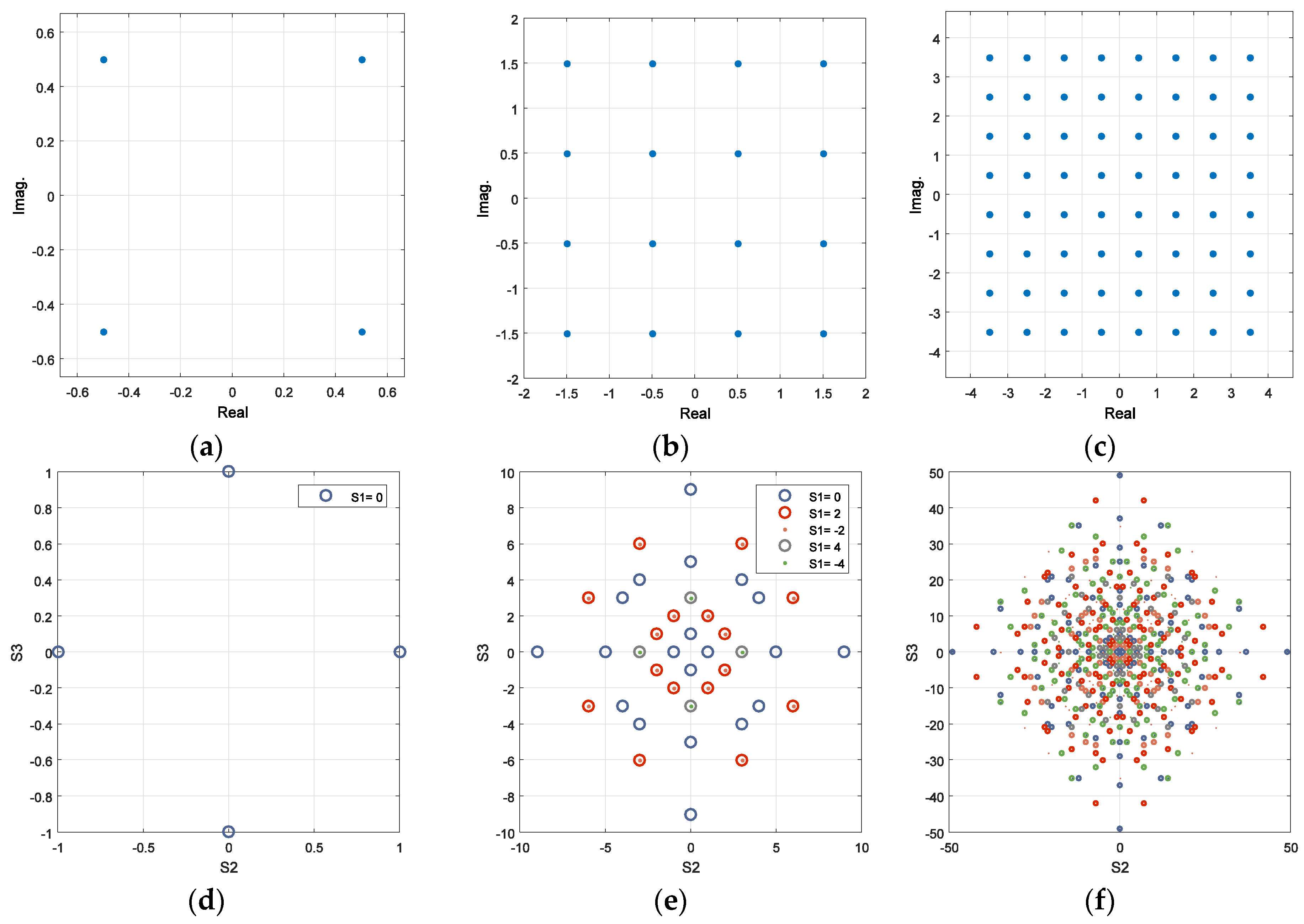
Although one dimension is lost in the Stokes transformation, its transformation can be effectively used for tracking signal impairments. Introduced by [6], the Stokes Space Algorithm (SSA) equalizer takes advantage of the Stokes transformation to calculate the error function in that domain. As a consequence of this non-injective transformation, the number of points of the constellation of the transformed stokes space are reduced by a factor of approximately four [23].

The advantages of Stokes space is that it is insensitive to frequency offsets and phase rotations simultaneously introduced in both polarizations [6]. The SSA computes the error function as described by:

$$f_{SSA}\left(h\left(n\right)\right)={||\overline{S}\left(n\right)-\widehat{\mathit{S}}\left(n\right)||}^2,$$

(7)

where $\overline{S}\left(n\right)$ and $\widehat{\mathit{S}}\left(n\right)$ are the vectors of the equalized and expected signal respectively expressed in the Stokes space.

For illustrative purposes, we include the comparison between the constellations in the Euclidean space, Figure 1a–c, and in the Stokes space, Figure 1d–f using the representation proposed by [23].

Moreover, the update coefficients of each polarization can be written as:

$$\begin{gathered} C_1\left(n\right)=4\left[{\overline{S}}_1\left(n\right)-\widehat{S_1}\left(n\right)\right]\overline{x}\left(n\right)+4\left[\left({\overline{S}}_2\left(n\right)-\widehat{S_2}\left(n\right)\right)+\sqrt{-1}\left({\overline{S}}_3\left(n\right)-\widehat{S_3}\left(n\right)\right)\right]\overline{\mathrm{y}}\left(n\right), \\ {C}_2\left(n\right)=4\left[\left({\overline{S}}_2\left(n\right)-\widehat{S_2}\left(n\right)\right)-\sqrt{-1}\left({\overline{S}}_3\left(n\right)-\widehat{S_3}\left(n\right)\right)\right]\overline{x}\left(n\right)-4\left[{\overline{S}}_1\left(n\right)-\widehat{S_1}\left(n\right)\right]\overline{y}\left(n\right). \end{gathered}$$

(8)

Since the Stokes transformation is a nonlinear transformation, the DD algorithm based on minimum distance results in a suboptimal implementation. Alternatively, a maximum likelihood (ML) rule can be applied at the expense of increasing computational complexity [24]:

$$\widehat{\mathit{S}}\left(n\right)={\underset{k}{\max }}^{-1}{f}_{\mathit{S}|\mathit{S}\left(k\right)}\left(\overline{\mathit{S}}\left(n\right)|{\mathit{S}}_{\left(k\right)}\right)={\underset{k}{\max }}^{-1}[-\frac{\left|\left|{\overline{\mathit{S}}}_{\left(k\right)}\right|\right|}{2{\sigma }^2}+log{I}_0\left(\frac{\sqrt{\left|\left|{\mathit{S}}_{\left(k\right)}\left|\left|\right|\right|\overline{\mathit{S}}\left(n\right)\right|\right|}}{{\sigma }^2}\cos \left(\frac{{\theta }_{\left(k\right)}}{2}\right)\right)],$$

(9)

where $I_0$ is the modified Bessel function of order zero, ${\theta }_{\left(k\right)}$ is the angle between the Stokes vectors ${\mathit{S}}_{\left(k\right)}$ and $\overline{\mathit{S}}\left(n\right)$, and ${\sigma }^2$ is the noise variance. Simplified approximations of the previous formula are also available for decreasing the computational complexity [6].

3.2. Multi-Mode 2M × 2M Dynamic Equalization

For the generalized equalization, we considered $M$ interfering propagating modes, resulting in an equalizer of 2M × 2M. The x and y polarizations of the $v$-mode of the received signal are denoted by ${\mathit{x}}_v^{\left(n\right)}$ and ${\mathit{y}}_v^{\left(n\right)}$. Similar to the 2 × 2 case, the equalization of the received signals can be expressed as [8]:

$$\begin{gathered} {\overline{x}}_v\left(n\right)={{\displaystyle \sum }}_{j=1}^{\mathrm{M}}{\mathit{x}}_j^{\left(n\right)}·{\mathit{h}}_{x_v{x}_j}^{\left(n\right)}+{\mathit{y}}_j^{\left(\mathrm{n}\right)}·{\mathit{h}}_{x_v{y}_j}^{\left(n\right)}, \\ {\overline{y}}_v\left(n\right)={{\displaystyle \sum }}_{j=1}^{\mathrm{M}}{\mathit{x}}_j^{\left(n\right)}·{\mathit{h}}_{y_v{x}_j}^{\left(n\right)}+{\mathit{y}}_j^{\left(\mathrm{n}\right)}·{\mathit{h}}_{y_v{y}_j}^{\left(n\right)}, \end{gathered}$$

(10)

where the filter coefficients are:

$$\begin{gathered} {\mathit{h}}_{x_v{x}_u}^{\left(n\right)}=\left[h_{x_v{x}_u}^{\left(n\right)}\left(1\right),h_{x_v{x}_u}^{\left(n\right)}\left(2\right)\dots h_{x_v{x}_u}^{\left(n\right)}\left(N\right)\right];{\mathit{h}}_{y_v{x}_u}^{\left(n\right)}=\left[h_{y_v{x}_u}^{\left(n\right)}\left(1\right),h_{y_v{x}_u}^{\left(n\right)}\left(2\right)\dots h_{y_v{x}_u}^{\left(n\right)}\left(N\right)\right], \\ {\mathit{h}}_{x_v{y}_u}^{\left(n\right)}=\left[h_{x_v{y}_u}^{\left(n\right)}\left(1\right),h_{x_v{y}_u}^{\left(n\right)}\left(2\right)\dots h_{x_v{y}_u}^{\left(n\right)}\left(N\right)\right];{\mathit{h}}_{y_v{y}_u}^{\left(n\right)}=\left[h_{y_v{y}_u}^{\left(n\right)}\left(1\right),h_{y_v{y}_u}^{\left(n\right)}\left(2\right)\dots h_{y_v{y}_u}^{\left(n\right)}\left(N\right)\right]. \end{gathered}$$

(11)

The input signals consist of a vector accounting for N samples of the received signal:

$$\begin{gathered} {\mathit{x}}_v^{\left(n\right)}=\left[x_v\left(n\right),x_v\left(n-1\right),\dots ,x_v\left(n-N+1\right)\right], \\ {\mathit{y}}_v^{\left(n\right)}=\left[y_v\left(n\right),y_v\left(n-1\right),\dots ,y_v\left(n-N+1\right)\right]. \end{gathered}$$

(12)

Similar to the single-mode equalizer, the filter coefficients are updated based on the stochastic gradient update rule, where the generalized equations describing the filter update are:

$$\begin{gathered} {\mathit{h}}_{l_d{m}_g}^{\left(n+1\right)}={\mathit{h}}_{l_d{m}_g}^{\left(n\right)}-\mu {\nabla }_{{\mathit{h}}_{l_d{m}_g}^{\left(n\right)}}f({\mathit{h}}^{\left(n\right)});l,m\in \left\{x,y\right\}, \\ {\nabla }_{{\mathit{h}}_{l_d{m}_g}^{\left(n\right)}}f({\mathit{h}}^{\left(n\right)})=C_{pd}\left(n\right){\mathit{m}}_{\mathit{g}}^{*\left(n\right)};p=\{\begin{array}{c}1,l=x\\ 2,l=y\end{array}. \end{gathered}$$

(13)

$C_{1d}$ and $C_{2d}$ correspond to the error functions of the mode d. For consistency, we introduce the LMS and SSA and their error functions for multi-mode equalization.

3.2.1. Least Mean Square

The error function of LMS is defined as:

$$f_{LMS,v}\left(h\left(n\right)\right)={\left|{\overline{x}}_v\left(n\right)-{\widehat{x}}_v\left(n\right)\right|}^2+{\left|{\overline{y}}_v\left(n\right)-{\widehat{y}}_v\left(n\right)\right|}^2,$$

(14)

where ${\widehat{x}}_v\left(n\right)$ and ${\widehat{y}}_v\left(n\right)$ are the expected signals of each mode $v$. Similar to the 2 × 2 case, the LMS equalizer can operate in training mode or decision-directed (DD) mode. According to our description of the stochastic gradient descent, the 2M × 2M LMS algorithm has the following error coefficients:

$$C_{1v}\left(n\right)=2\left({\overline{x}}_v\left(n\right)-{\widehat{x}}_v\left(n\right)\right)\overline{x_v}\left(n\right);C_{2v}\left(n\right)=2\left({\overline{y}}_v\left(n\right)-{\widehat{y}}_v\left(n\right)\right){\overline{y}}_v\left(n\right).$$

(15)

3.2.2. Stokes Space Algorithm

The generalization of the SSA algorithm to 2M × 2M computes the error function into the Stokes space for each mode:

$$f_{SSA,v}\left(h\left(n\right)\right)=||{\overline{\mathit{S}}}_v\left(n\right)-{\widehat{\mathit{S}}}_v\left(n\right)|{|}^2,$$

(16)

where ${\overline{\mathit{S}}}_v\left(n\right)$ and ${\widehat{\mathit{S}}}_v\left(n\right)$ are the equalized and expected signal respectively of the mode $v$ expressed in the Stokes domain. Moreover, the generalized update coefficients of the 2M × 2M SSA equalizer are:

$$\begin{gathered} C_{1v}\left(n\right)=4\left[{\overline{S}}_{1v}\left(n\right)-\widehat{S_{1v}}\left(n\right)\right]{\overline{x}}_v\left(n\right)+4\left[\left({\overline{S}}_{2v}\left(n\right)-\widehat{S_{2v}}\left(n\right)\right)+\sqrt{-1}\left({\overline{S}}_{3v}\left(n\right)-\widehat{S_{3v}}\left(n\right)\right)\right]{\overline{y}}_v\left(n\right), \\ {C}_{2v}\left(n\right)=4\left[\left({\overline{S}}_{2v}\left(n\right)-\widehat{S_{2v}}\left(n\right)\right)-\sqrt{-1}\left({\overline{S}}_{3v}\left(n\right)-\widehat{S_{3v}}\left(n\right)\right)\right]x_v\left(n\right)-4\left[{\overline{S}}_{1v}\left(n\right)-\widehat{S_{1v}}\left(n\right)\right]{\overline{y}}_v\left(n\right). \end{gathered}$$

(17)

4. Frequency Domain Equalization

Due to signal impairments such as DMGD, SDM systems may much have longer impulse responses, resulting in an increment of the number of taps of the equalizer [25]. In addition, multi-mode equalization systems with M modes need M² times as many filters compared to single-mode equalization. Hence, the computational complexity is increased dramatically and efficient implementations of the MIMO equalization are required to overcome the increase of the number of taps and filters in multi-mode equalization.

A well-known approach to decrease the computational complexity is the frequency domain (FD) equalization [26]. The FD equalization is rooted in the equivalence of time domain (TD) convolutions and multiplications in FD, allowing to effectively reduce the number of arithmetic operations of the equalizer [7].

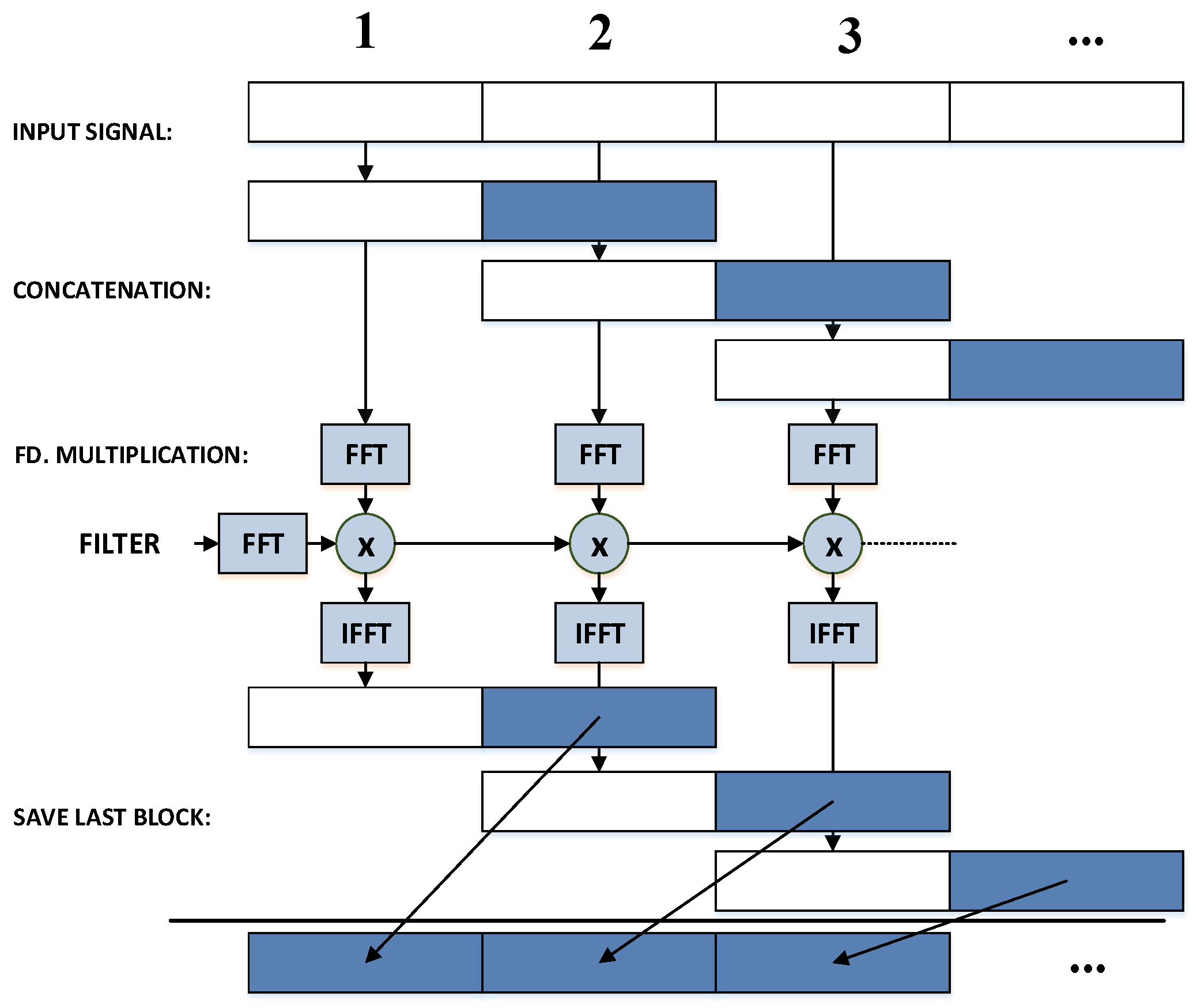
As multiplications in FD correspond to cyclic but not linear convolutions in TD, different methods have been introduced to resolve this issue: most common ones are the overlap-save and the overlap-add techniques [27]. In this paper, we focus on the overlap-save, but similar results are expected from the overlap-add technique.

Figure 2 illustrates the overlap-save technique, where two blocks are concatenated together. The light blue color is used to differentiate the last block from the initial one. For simplicity, same length is assumed for both blocks. The concatenated signals are Fourier-transformed to FD, where they are multiplied by the filter coefficients also expressed in FD. Once the multiplications are performed, the resultant signals are converted back to TD. The initial block is discarded, while the last block is the result of the desired linear convolution, and hence saved.

The single- and multi-mode equalizations previously explained can be written in FD as:

$$\begin{gathered} {\overline{\mathit{X}}}_v^{\left(n\right)}={{\displaystyle \sum }}_{j=1}^M{\mathit{X}}_j^{\left(n\right)}*{\mathit{H}}_{x_v{x}_j}^{\left(n\right)}+{\mathit{Y}}_j^{\left(n\right)}*{\mathit{H}}_{x_v{y}_j}^{\left(n\right)}, \\ {\overline{\mathit{Y}}}_v^{\left(n\right)}={{\displaystyle \sum }}_{j=1}^M{\mathit{X}}_j^{\left(n\right)}*{\mathit{H}}_{y_v{x}_j}^{\left(n\right)}+{\mathit{Y}}_j^{\left(n\right)}*{\mathit{H}}_{y_v{y}_j}^{\left(n\right)}, \end{gathered}$$

(18)

where ${\mathit{X}}_v^{\left(\mathrm{n}\right)}$, ${\mathit{Y}}_v^{\left(\mathrm{n}\right)}$ are the input signals of the received mode $v$, ${\mathit{H}}_{x_v{x}_j}^{\left(n\right)}$, ${\mathit{H}}_{x_v{y}_j}^{\left(n\right)}$, ${\mathit{H}}_{y_v{x}_j}^{\left(n\right)}$, ${\mathit{H}}_{y_v{y}_j}^{\left(n\right)}$ are the filter coefficients and ${\overline{\mathit{X}}}_v^{\left(n\right)}$, ${\overline{\mathit{Y}}}_v^{\left(n\right)}$the result of the equalization. The notation $‘*’$ is defined as the element wise multiplication of the vectors: $\mathit{A}*\mathit{B}=\left[a_1{b}_1,\dots ,a_n{b}_n\right]$. As defined by the overlap-save technique, the input signal vectors are formed by two blocks concatenated and transformed into the Fourier domain:

$${\mathit{X}}_v^{\left(n\right)}=FFT\left\{\left[{\mathit{x}}_v^{\left(n-1\right)},{\mathit{x}}_v^{\left(n\right)}\right]\right\};{\mathit{Y}}_v^{\left(n\right)}=FFT\left\{\left[{\mathit{y}}_v^{\left(n-1\right)},{\mathit{y}}_v^{\left(n\right)}\right]\right\}.$$

(19)

The ‘$\left[\mathit{a},\mathit{b}\right]$’ operation represents the concatenation of vectors $\mathit{a}$ and $\mathit{b}$; and ‘$FFT${}’ is the Fourier transform operator. The response of the frequency domain filter is limited by a constraint $\mathit{K}$ [27], which limits the non-zero filters coefficients to a certain range in order to speed up the convergence:

$${\mathit{H}}_{l_d{m}_g}^{\left(n+1\right)}=FFT\left\{\mathit{K}*IFFT\left\{{\mathit{H}}_{l_d{m}_g}^{\left(n\right)}\right\}\right\};l,m\in \left\{x,y\right\};d,g\in \left[1,M\right].$$

(20)

Finally the equalized signal in TD (${\overline{\mathit{x}}}_v^{\left(n\right)}$,${\overline{\mathit{y}}}_v^{\left(n\right)}$) is obtained by IFFT of the FD signal as:

$$\begin{gathered} {\overline{\mathit{x}}}_v^{\left(n\right)}{}^{\prime }=IFFT\left\{{\overline{\mathit{X}}}_v^{\left(n\right)}\right\};{\overline{\mathit{y}}}_v^{\left(n\right)}{}^{\prime }=IFFT\left\{{\overline{\mathit{Y}}}_v^{\left(n\right)}\right\}, \\ {\overline{\mathit{x}}}_v^{\left(n\right)}=E_{N+1}^{2N}\left({\overline{\mathit{x}}}_v^{\left(n\right)}{}^{\prime }\right);{\overline{\mathit{y}}}_v^{\left(n\right)}=E_{N+1}^{2N}\left({\overline{\mathit{y}}}_v^{\left(n\right)}{}^{\prime }\right). \end{gathered}$$

(21)

As explained before, the last block—i.e., the last N samples—of the signal should be extracted. This operation is denoted by the operator$E_{N+1}^{2N}$. The equalized signals are compared to the expected signals according to the described error functions to obtain the error coefficients: ${{\mathit{C}}_{1v}}^{\left(n\right)}$ and${{\mathit{C}}_{2v}}^{\left(n\right)}$. Since our equalizers are based on unfolded signals of two samples per symbol, the update coefficients of the non-optimum sampling point are filled with zeros. 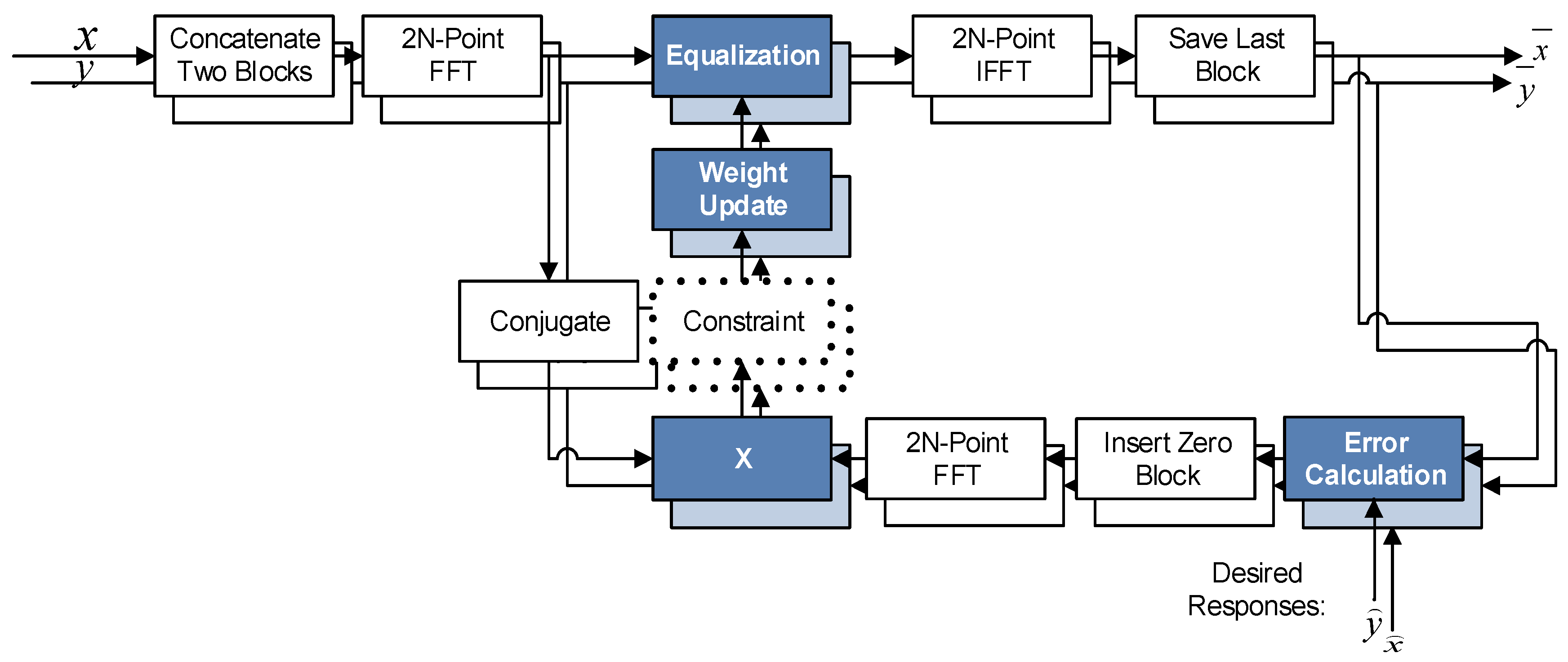Figure 3 illustrates the 2 × 2 equalization performed in FD.

5. Results

The evaluation of the equalization techniques presented in this paper is done by computer simulations. We focus on the performance of the FD implementations of both algorithms considering two different setups: a single-mode setup for 2 × 2 equalization, for those SDM scenarios with no or negligible modal impairments; and a multi-mode setup consisting of three modes requiring 6 × 6 equalization. The two setups modelled by computer simulations have the following specifications:

• SSMF transmission, consisting of a 32 Gbaud non-return-to-zero (NRZ) dual-polarization QPSK signal, modelling the signal impairments of SoP rotation, PMD, polarization dependent loss (PDL) and CD.
• Three mode transmission over FMF, consisting of three decorrelated replicas of the same 32 Gbaud QPSK signal. Besides those impairments in SSMF, mode mixing and DMGD are also considered.

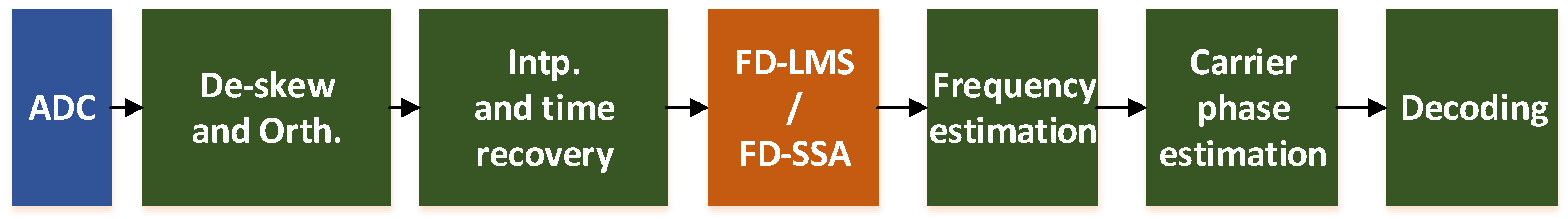
The implemented DSP stack is shown in Figure 4, beginning with de-skewing the received signal and compensating possible imbalances of the 90° hybrids by orthonormalization. Then, interpolation and time-recovery are applied to obtain a 2-sample per symbol signal, followed by the FD-LMS or FD-SSA, compensating for the mode mixing and signal impairments. Frequency-offset and phase noise are compensated by a 64-taps Viterbi-and-Viterbi [28] and the differential Viterbi-and-Viterbi algorithms [1]. Finally, the received signal is decoded and the bit-error rate (BER) is calculated.

All the simulations are performed with random blocks of 1 million symbols, where the number of iterations used for equalization is adjusted for each case. The accumulated CD employed was smaller than the equalizer size for each case for avoiding penalties.

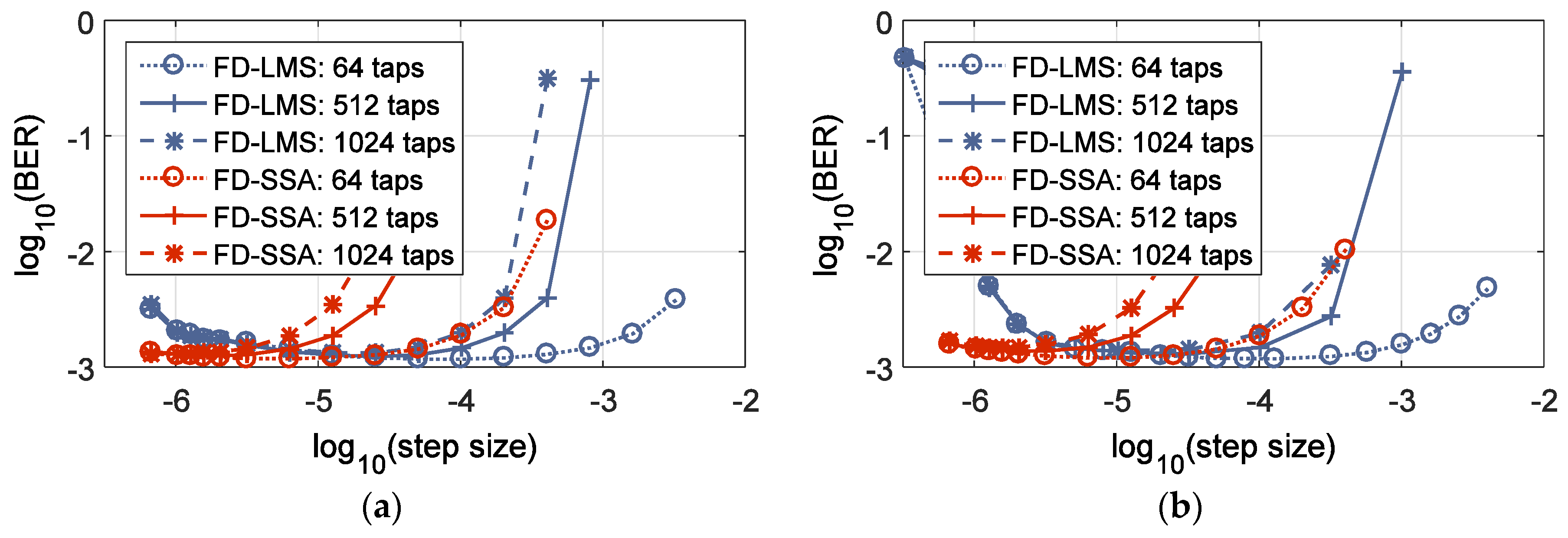
5.1. Step Size Optimization

Since the MMF transmission generally results in longer impulse response, we evaluate our system with 3 different equalizer lengths: 64-taps, 512-taps, and 1024-taps, corresponding to 32-taps, 256-taps, and 512-taps of a TD equalizer, respectively.

Figure 5 shows the optimization of the step-size for the considered algorithms: (a) single-mode equalization and (b) multi-mode equalization. It can be observed that the optimum step-size decreases with the number of taps considered.

Table 1. Step sizes used for the different equalizers considered.

	64 Taps	512 Taps	1024 Taps
2 × 2 FD-LMS	10−3.4	10−4.3	10−4.6
2 × 2 FD-SSA	10−4.6	10−5.5	10−5.7
6 × 6 FD-LMS	10−3.5	10−4.5	10−4.7
6 × 6 FD-SSA	10−4.6	10−5.5	10−5.8

sums up the optimum step-sizes for FD-SSA and FD-LMS for the 2 × 2 and 6 × 6 case.

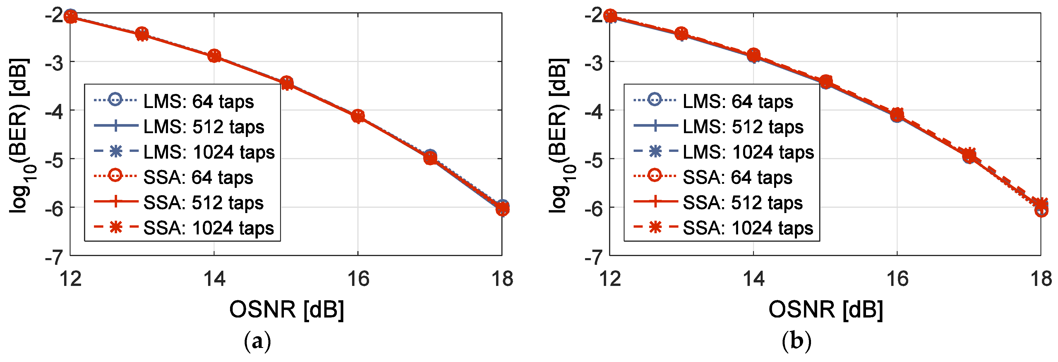
5.2. BER vs. OSNR

Once the step-size is optimized, we evaluate the performance for different optical signal-to-noise ratios (OSNR). In order to track the phase, a carrier-phase estimation (CPE) with a windows size of 64 taps is included for both FD-LMS and FD-SSA (see Figure 4).

Figure 6 compares the BER performance of the FD-LMS and FD-SSA algorithms for both 2 × 2 and 6 × 6 implementations. It is observed that FD-LMS and FD-SSA achieve almost identical performance.

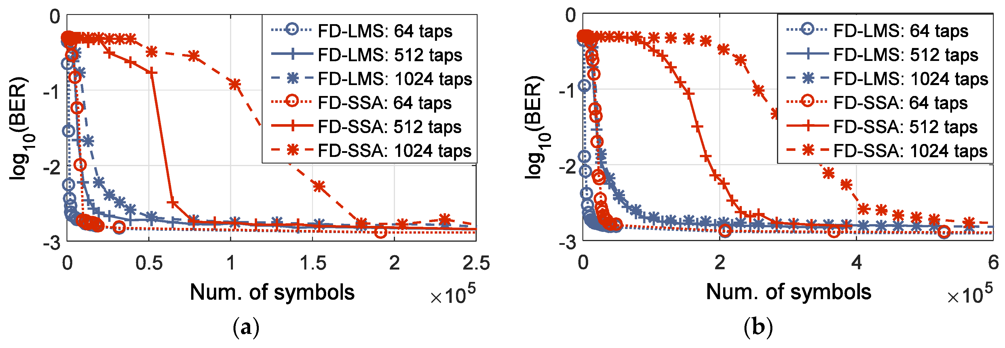
5.3. Convergence Speed

The convergence speed determines the amount of symbols needed to obtain adequate performance of the equalizer, allowing the successful compensation of the signal impairments. Figure 7 shows the convergence speed of the FD implementation for both SSA and LMS. Figure 7a presents the 2 × 2 case while Figure 7b shows the 6 × 6. For both FD-LMS and FD-SSA the number of symbols required for equalization is increased when switching from 2 × 2 to 6 × 6 equalization. Furthermore, in both cases, SSA equalizer is more sensitive to the number of taps of the equalizer, i.e., its convergence speed reduces significantly with increasing the number of taps.

Table 2. Number of symbols required (× 10⁻³) for convergence (approx.).

	64 Taps	512 Taps	1024 Taps
2 × 2 LMS	8	38	76
2 × 2 SSA	10	76	180
6 × 6 LMS	12	100	128
6 × 6 SSA	32	250	500

shows the required number of symbols to achieve convergence in each case.

5.4. Frequency Offset

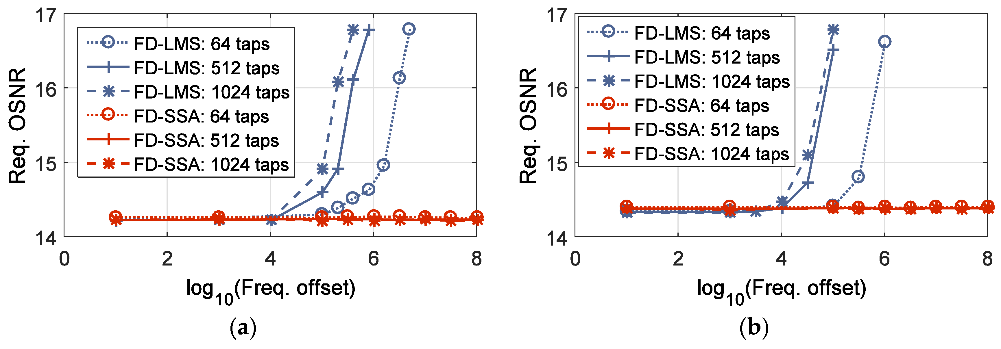
The effect of the linewidth for the FD-SSA and FD-LMS was already studied in [8] for the 6 × 6 case. In this paper, we study the effect of the frequency offset. Figure 8 shows the required OSNR (ROSNR) for BER 10⁻³ as a function of the frequency offset. Due to the block nature, LMS with larger number of taps is more sensitive to frequency offset and requires higher OSNR for achieving the same BER performance as SSA.

Figure 8 also confirms that the frequency offset introduces a slightly higher penalty for the 6 × 6 equalization compared to the 2 × 2 for the FD-LMS equalizer. The FD-SSA is insensitive to frequency offsets, which is reflected by constant ROSNR, independent of the equalizer filter length.

6. Conclusions

In this paper, we reviewed different equalization techniques for SDM transmission systems. Efficient implementations of the proposed equalization algorithms in FD were also studied.

We introduced the novel FD-SSA and its corresponding MIMO implementation, and compared it to the FD-LMS in terms of performance (OSNR-BER), convergence speed, and frequency offset tolerance. The main advantage of the FD-SSA filter update rule is its insensitivity to frequency offsets and phase noise. SSA equalizer can effectively achieve convergence in scenarios with high frequency offsets and linewidths, which may result in instabilities for the FD-LMS equalizer.

However, SSA suffers from slow convergence for big number of taps. Therefore implementations of the SSA based on algorithms capable of speeding up the convergence, such as the power-directed or the noise-directed filter update rule [29], may be desired in the future. Another alternative is reducing the impulse response by careful fiber design. Those systems may take advantage of SSA equalization technique without needing further optimization of the convergence speed.