XL-SIM: Extending Superresolution into Deeper Layers

1
Bio Imaging Zentrum der Ludwig-Maximilians-Universität München, 82152 Martinsried, Germany;
2
TILL I.D. GmbH, 82152 Planegg/Martinsried, Germany
*
Authors to whom correspondence should be addressed.
Photonics 2017, 4(2), 33; https://doi.org/10.3390/photonics4020033
Submission received: 14 March 2017
/
Revised: 7 April 2017
/
Accepted: 13 April 2017
/
Published: 20 April 2017
(This article belongs to the Special Issue Superresolution Optical Microscopy)
Abstract
:Of all 3D-super resolution techniques, structured illumination microscopy (SIM) provides the best compromise with respect to resolution, signal-to-noise ratio (S/N), speed and cell viability. Its ability to achieve double resolution in all three dimensions enables resolving 3D-volumes almost 10× smaller than with a normal light microscope. Its major drawback is noise contained in the out-of-focus-signal, which—unlike the out-of-focus signal itself—cannot be removed mathematically. The resulting “noise-pollution” grows bigger the more light is removed, thus rendering thicker biological samples unsuitable for SIM. By using a slit confocal pattern, we employ optical means to suppress out-of-focus light before its noise can spoil SIM mathematics. This not only increases tissue penetration considerably, but also provides a better S/N performance and an improved confocality. The SIM pattern we employ is no line grid, but a two-dimensional hexagonal structure, which makes pattern rotation between image acquisitions obsolete and thus simplifies image acquisition and yields more robust fit parameters for SIM.
1. Introduction
In widefield epifluorescence microscopy, image contrast and resolution is impaired by fluorescence emission originating from layers above and below the focus plane [1] (out-of-focus). The gold-standard for curing this problem is the confocal microscope, which employs optical means i.e., a pinhole for rejecting out-of-focus light. A totally different cure for the same problem is provided by structured illumination microscopy (SIM). Here, a structured illumination pattern is used for excitation and the emission is detected without a pinhole. By recording several raw images at different pattern positions on the sample, the out-of-focus emission can be removed computationally from the recorded raw images [2,3]. The phase shifted SIM raw images are called phase images in the following.
While the resolution of an optical microscope depends on the minimum distance of two distinguishable radiating points, confocality describes its sectioning power, i.e., its ability to suppress out-of-focus information [4,5]. With respect to confocality, SIM outperforms every confocal microscope [6]. On top of that, it has the potential to increase the resolution beyond the Rayleigh limit [7,8,9,10]. While this resolution enhancement is not as great as with other super resolution techniques like e.g., PALM [11], STORM [12] or STED [13], SIM provides several distinct advantages:
Thus, SIM appears to provide the most viable path to (3D)-super resolution when resolution gain is weighed against speed, signal-to-noise ratio (S/N) and the capability to examine live cells in two [17] and in three dimensions [15]. However, the S/N of SIM is compromised by the detected out-of-focus signal [18], an effect which increases with sample thickness and with increased extent of staining. This has limited the usage of 3D-SIM to samples no thicker then a few micrometers. Here, we present a novel concept which combines SIM with line-confocal detection (L-SIM), thus optically reducing the amount of out-of-focus information before mathematics remove the rest. This way we allow SIM to go significantly deeper without compromising the signal-to-noise ratio.
Commercial SIM systems [19] and most other SIM approaches [9,10,20,21,22] employ line grid patterns. For super resolution, these patterns need to be rotated to at least three different orientations in order to obtain an increased resolution in all directions of the image plane. In order to extend super resolution SIM to three dimensions, sets of phase images at different grid positions and orientations have to be recorded for several z-positions. This way, a resolution improvement by a factor of two can also be achieved in a z-direction [21].
Given that the precision of all three parameters (grid position, grid orientation and z-position) critically enters the most crucial steps in the evaluation of SIM images/3D-SIM volumes, namely, determination of the frequency vectors of the pattern changes calculation of the images. This needs to be performed for every SIM image processing, and any error here will lead to artifacts as well as to a reduction of resolution in the final processed image.
In the following, we shall present a combination of two-dimensional hexagonal patterns for SIM (hexagonal SIM = X-SIM) [23] with line-confocal detection (line-confocal SIM = L-SIM), called hexagonal line-confocal SIM (XL-SIM) as a powerful super resolution tool for live cell imaging. While two-dimensional SIM patterns have been described before [24,25], the novelty of our approach lies in the fact that we need to shift the grid pattern in one dimension only between phase image acquisitions [23]. The other novelty lies in the confocal spatial filtering, which improves confocality and—by discarding out-of-focus emission in the detected phase images—makes SIM more applicable to thicker samples.
2. Results
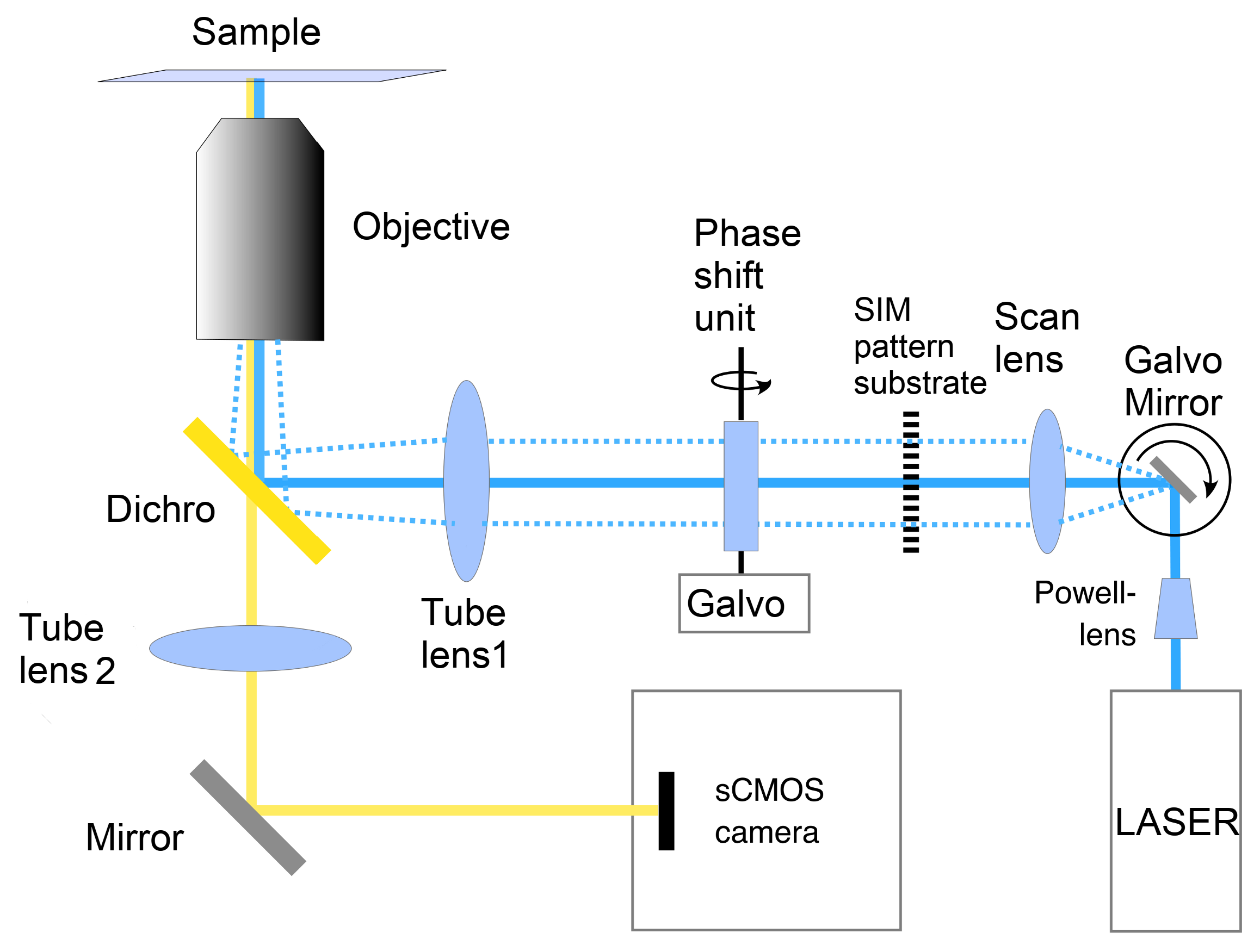
In order to achieve a line-confocal excitation, we scan a laser-line over the SIM-pattern substrate and image the latter onto the sample. The laser line is generated by a Powell lens (for details, see methods Section 4.1 and the drawing in Figure 1). The result is a two-dimensionally modulated intensity profile, which—for a given region of the sample—lights up and subsequently fades again as the laser-line sweeps over the corresponding area of the pattern mask. An sCMOS camera chip with a rolling shutter is used for detection, and the movement of the structured excitation line is synchronized with the movement of the rolling shutter active pixel area. Thus, unlike in previously described combinations of SIM with line-confocal microscopy [22], phase images are obtained in a single sweep, which, in the experiments shown, takes no more than 10 for a field of pixels.
2.1. Theory
To generate an intensity profile with hexagonal modulation, a binary phase pattern with hexagonal symmetry and a phase step of is placed into the intermediate image-plane of the microscope’s excitation beam path. Here, it was designed to produce hexagonal diffraction orders for the excitation wavelength nm, with zero order contain about 70–80% of the power of the first diffraction orders, as described in [21] (for details, see Supplementary Note 5 and Supplementary Figure S5). Given that the pattern contrast is caused by interference, the laser line focus must encompass a minimum width. A narrower focused line would reduce interference in the direction orthogonal to the line and would thus reduce pattern contrast in this direction.
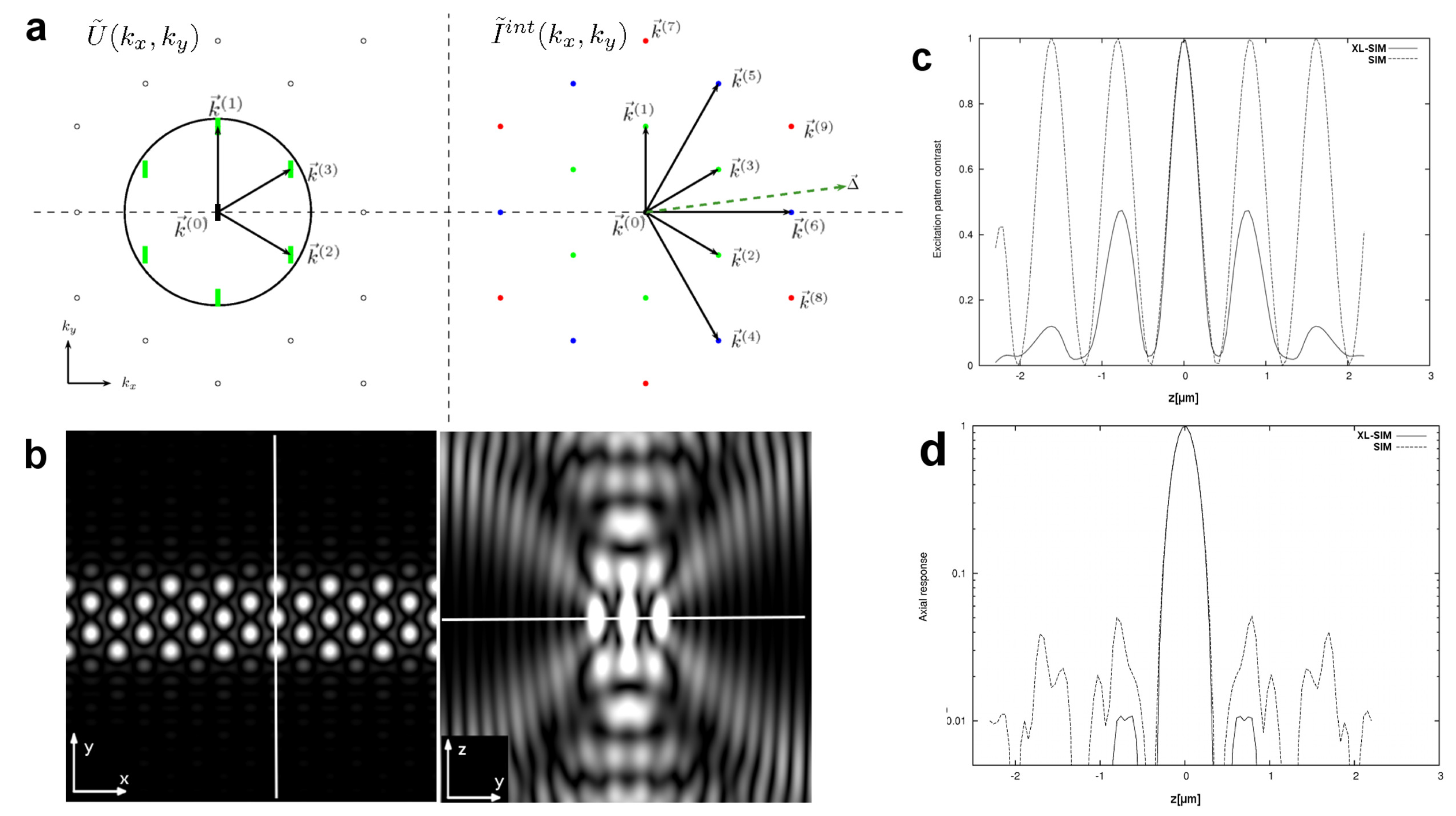
A similar effect is illustrated in Figure 2a, where the hexagonal diffraction orders are broadened in one direction by the line shaped excitation. Reducing the line width relative to the pattern period, would increase confocality, but at the expense of modulation depth of the hexagonal pattern frequencies of the integrated excitation intensity , shown on the right in Figure 2a. Reducing the pattern frequency to overcome this would—in turn—increase modulation depth again, but at the expense of a reduced resolution. This means that there is a trade-off between pattern frequency (resolution) and excitation line width of the laser focus (confocality). In the present experiments, our main emphasis was on resolution, hence the pattern base frequency was chosen slightly below the microscope objective’s cut-off frequency and the full-width-at-half-maximum of the excitation line focus width was approximately 3 pattern periods, as described in Supplementary Note 2 and Supplementary Figure S4. The sectioning ability of a microscope, also called confocality, is defined as the axial response to a thin fluorescent layer to defocussing action [6]. Several methods to quantify confocality have been introduced, e.g., in [4,5], they all encompass measuring z-stacks of a thin fluorescent sheet. In SIM microscopy, the axial response depends on the pattern contrast as a function of defocus. In cases where the whole area of interest is illuminated simultaneously—as in conventional (3D)SIM—several planes of excitation contrast exist due to the Talbot-effect, they are called Talbot planes. The axial extent of the excitation contrast (or equivalently the number of Talbot planes) is limited by the spatial coherence of the excitation laser light [21]. In contrast to conventional line grid SIM, the location of local intensity maxima in all Talbot planes corresponds to their location in the main focus plane with hexagonal patterns.
With line-confocal excitation, this is different as illustrated in Figure 2b: there is a symmetry break in the hexagonal pattern intensity, which causes the local maxima of the Talbot planes to shift towards the center of the excitation line. Thus, moving the line across the pattern substrate leads to moving local intensity maxima in the Talbot planes, but not in the focus plane. This is illustrated in Supplementary Video 1 and further explained in Supplementary Figure S2. As a consequence, the integrated excitation pattern contrast is reduced in the Talbot planes above and below the focus plane, and this, in turn, leads to improved confocality and axial z-resolution of XL-SIM. This is shown in Figure 2c, which depicts mathematical simulations of the integrated excitation contrast as a function of defocus for conventional SIM and XL-SIM illumination at nm. The objective entered into the simulation was a NA 1.4 oil immersion. A plot of the simulated axial response (confocality) for XL-SIM and SIM is shown in Figure 2d.
The height of the rolling shutter window determines line-confocality. It can be chosen narrower than the excitation line; in the simulation, it was assumed to be two hexagon periods, which corresponds to approximately 10 camera pixels or an exposure time of 100 in the fast mode of the camera. The reduced excitation contrast in the Talbot layers leads to a reduced axial response in these layers and thus better confocality when using XL-SIM.
Hexagonal SIM
In order to separate all spatial frequency bands contained in the detected signal, several phase images have to be recorded and the pattern has to be phase shifted between phase images. As described in [23], it is sufficient to shift the hexagonal pattern along one spatial direction, provided one chooses the right angle between the pattern symmetry axes and the shift direction so as to allow separation of all frequency bands contained in the detected phase images with a unitary matrix. The angle depends on the number of frequency orders contained in the excitation intensity spectrum.
The period of the hexagonal pattern is chosen such that only the seven first diffraction orders of the hexagonal pattern can pass the microscope objective pupil. As illustrated in Figure 2a and Supplementary Figure S3, these seven first diffraction orders will interfere to totally 19 frequency orders in the excitation intensity spectrum, oriented in six different directions. Further details about the hexagonal frequencies and the shift direction can be found in Supplementary Note 1.
Assuming linear fluorescence excitation, the m-th recorded XL-SIM phase image can thus be written as follows:
denotes the modulation of the n-th frequency order on a pixel , and is the unmodulated background signal. The relative phase shift (i.e., the phase shift in the m-th recorded phase image relative to the first one) is given by and is the absolute phase of the n-th frequency in the first recorded image, which only depends on the origin of the chosen coordinate system. The Fourier transform of Equation (1) is consequently given by the superposition of 19 so called frequency bands , which correspond to 19 unknowns. Thus, a minimum of 19 phase images have to be recorded for solving all frequency bands contained in the phase images .
In the above scheme, the rolling shutter width not only determines the camera exposure time, but also the degree of slit-confocality for a given phase image. Thus choosing a narrow rolling shutter width to obtain better confocality—to account for increased sample thickness, for example—also reduces the time the sample is exposed to excitation light in a given phase-image scan. To increase signal strength, again in case of weak fluorescence signals, one can resort to a slower scan-mode of the camera or increase the number of recorded phase images beyond the minimum number. The minimum acquisition time of the PCO Edge camera (pco.edge 4.2) (Kelheim, Germany) for one XL-SIM phase image amounts to 10 , for a full frame image () pixels. If fewer camera lines are read out, the total acquisition time is reduced accordingly. Thus, a field of pixels corresponding to an area of 1000 m2 can be imaged within 30 ms. With an image stack consisting of 100 layers, spaced 100 nm apart, one can record a 10,000 m3 XL-SIM image volume in 2 s.
By mounting the hexagonal phase substrate on a rotatable disc, it is possible to adjust the pattern-orientation relative to the shift-direction. Unless the disk-rotation is used to insert alternative patterns into the beam path, the correct pattern orientation does not need to be changed anymore. The pattern frequency vectors can be calibrated e.g., using a thin layer of fluorescent dye, as also used in [4]. Calibration is performed by pairwise comparison of the phase shifts of the hexagonal frequency orders in the phase images.
In most SIM approaches and commercial solutions, line grid patterns are used for SIM, which must be rotated to at least three orientations and a minimum number of at least five phase images have to be recorded for every orientation [21]. After solving the system of linear equations for these unknown frequency bands, the bands have to be shifted to their original positions in Fourier space. These shifts require quite precise knowledge of the pattern frequency vectors. When the frequency bands are at their original positions, their values can be compared (respecting the influence of the microscope objective emission OTF) with the 0th frequency band in order to determine a complex factor (which is called in [21]) for each frequency band. These factors reflect the contrast of the n-th pattern frequency in the sample () as well as the absolute position (phase) of the n-th pattern frequency in the first recorded phase image (). They are essential for the correct superposition of the frequency bands.
As a consequence, errors in the frequency vectors will lead to errors in the determined phase factors and to errors in the superposition itself because overlapped frequency values of the object don’t match. Errors of the frequency vector will lead to inhomogeneities across the SIM image. Errors of the phase factors (especially errors of ) will lead to a loss of information and will deteriorate the resolution that can be reached in the final processed SIM image/volume (see Supplementary Note 3 and Supplementary Figure S7).
Because the orientation of the pattern changes in every measurement, the frequency vectors have to be determined in every measurement directly from the measured data [21].
In contrast to the conventional SIM solutions with line grids, the frequency vectors can be kept invariant when using a hexagonal pattern for SIM. Thus, the determination of the pattern frequency vector becomes a calibration step. The only parameter that has to be fitted in the SIM processing is the complex factor () for each frequency band. Furthermore, only one z-stack of phase images has to be recorded instead of three when using line-grid SIM patterns. This avoids any possible errors in the z-positions of recorded layers, which can occur for thick samples/large z-stacks.
A consequence of an interferometric pattern contrast generation is its dependence on the polarization of the interfering waves [26]. Using a line grid pattern and linearly polarized light, the polarization can be adapted to the different pattern orientations. Using hexagonal patterns with linearly polarized light leads to different levels of contrasts for the different pattern intensity frequencies. This can be accounted for in the SIM processing [27], but the frequency bands exhibiting less contrasts will contribute more noise to the final processed image, especially in the higher order frequency bands which are essential for the resolution improvement.
However, this S/N degrading effect is more than compensated for by the following difference between 1D and 2D patterns: when line grids are used for SIM, only phase images for one pattern orientation are used for the calculation of frequency bands, which correspond to this pattern orientation. For example, if a total of phase images is recorded, there are five phase images recorded for each of the three pattern orientations and only five (of 15) images are used to calculate any non-zero frequency band. In contrast to the 0th frequency band, which is obtained three times, all other frequency bands are calculated by image data that corresponds to of the total exposure time. Hexagonal SIM allows for using all phase images for the calculation of all frequency bands and the 0th frequency band is obtained only once. This gives an improvement of S/N by a factor of when using X-SIM.
In essence, the polarization dependent effect on S/N is compensated by a three times lower variance in the non-zero frequency bands, thus the S/N for X-SIM is theoretically at least as good as for conventional SIM with line grids. The S/N situation can probably be further improved by using azimuthal instead of linear polarization.
2.2. Resolution Doubling by XL-SIM
In order to test the resolution of XL-SIM qualitatively, we used a tubulin sample. Further information about this sample can be found in the Material and Methods section.
A z-stack of phase images was recorded with a total number of 19 phase images in each layer. Thus, the total acquisition time was 190 for every layer for all required phase images. Because the sample thickness amounts to only a few micrometers, the rolling shutter width has been set to a value of 500 pixels. Thus, the phase images have been detected non-confocally. The resulting images permit illustrating the effect of out-of-focus removal by XL-SIM as compared to the calculated (quasi-) wide field (WF) images . Figure 3 shows a comparison of a XL-SIM image (a) with a WF image (b) of the tubulin sample.
2.3. SIM Image Reconstruction
The XL-SIM image has been calculated by separation of all 19 frequency bands that are contained in the phase images (compare Equation (1)). The complex factor is then determined for every frequency band and the frequency bands are shifted along their corresponding pattern frequency vectors in Fourier space. In order to provide enough space for shifting the frequency orders, the Fourier space images/volumes have to be padded with zeros before the shifts are applied. This is equivalent to a pixel interpolation. Usually, the evaluated pixels sizes are half of the camera pixel sizes [10,21].
Finally the frequency values of all bands are superimposed, according to Equation (2), which is a generalized Wiener filter [20,21,28,29]:
denotes the optical transfer function (OTF) of the n-th frequency band, which is shifted along the frequency vector . The parameter is the Wiener parameter, which has been chosen empirically and is an apodization function [21,29].
Apart from the shifts, the OTFs only differ concerning their functional dependency in the -direction of frequency space. In contrast to conventional SIM, the OTFs in Equation (2) depend on the confocality of the detection i.e., the rolling shutter width. Furthermore, their functional dependency on the direction depends on the excitation contrasts of the hexagonal frequencies as functions of defocus.
All XL-SIM images have been calculated according to Equation (2) without any further deconvolution. Figure 3c,d shows the region of interest (ROI) that is marked by `1’ for XL-SIM and WF. As one can see, this ROI hardly contains any out-of-focus emission and the XL-SIM image shows several features of the sample that are unresolved in the WF image. The contrast enhancement along the white horizontal lines in Figure 3c,d is illustrated as line profile plot in Figure 3g. Note that the intensity profile of the WF image has been scaled and an offset has been subtracted in order to overlap the intensity profiles for comparison. Figure 3e,f shows the enlarged ROI `2’. In contrast to ROI `1’, ROI `2’ contains detected out-of-focus emission, which leads to a loss of resolution in the WF image. The S/N in the evaluated XL-SIM image will be smaller for areas of the sample where more out-of-focus emission is detected, which finally also means a loss of resolution in these sample areas.
2.4. Quantitative Resolution Measurement
The resolution of XL-SIM has also been tested quantitatively in two different ways: with nanorulers from the company Gattaquant and with fluorescent microspheres from the company ThermoFisher.
Nanorulers are based on DNA origamis and consist of two distinct fluorescent marks separated by a fixed distance, which is 120 nm for the nanorulers we used in our experiments. They offer a convenient way to test respectively optimize the resolution of a microscope system. Figure 4a,b shows evaluated nanoruler images for WF and XL-SIM. The latter clearly resolves the two parts of the nanorulers. To provide a smoother image reconstruction, we employed a mathematical pixel interpolation factor of 4, bringing the pixel size in the reconstructed images down to 21 . For better comparison of WF with XL-SIM images, the same pixel-interpolation was also applied to the WF image in Figure 4a. Because the nanoruler sample is very thin (only one layer of nanorulers), we used non-line-confocal detection i.e., a rolling shutter width of ≈500 pixels. As each nanoruler carries only of a few molecules, laser intensity was reduced to avoid bleaching and the total exposure time was set to 760 by recording a set of 76 phase images for a given z-layer.
A criterion for the quantification of resolution, which is often used in the field of scanning electron microscopy, is Fourier-ring-correlation (FRC) [30]. FRC has also recently been used in optical microscopy [31,32]. A set of 76 phase images was split into two statistically independent sets of 38 phase images and two independent XL-SIM images were processed, which are shown in Supplementary Figure S12. Subsequently, the FRC was calculated from the two XL-SIM images of the nanoruler sample as described, e.g., in [31]. We used the value of as the threshold criterion, which has also been used, e.g., in [32]. A graphical illustration of the FRC is shown in Figure 4c. The FRC drops below the threshold for a distance of 106.1 . This determined resolution value approximately corresponds to the theoretically expected value for a doubled resolution, which is approximately 100 .
Another method for the quantification of resolution is the analysis of the microscope PSF as the image of point light sources. We used fluorescent microspheres with a diameter of approximately 50 nm, which is far below the expected resolution. A z-stack of phase images was recorded, and 19 phase images were recorded in every layer. The rolling shutter width was set to the minimum value of 10 pixels in order to get line-confocal detection (LC). Figure 4d,e shows corresponding views of the LC and XL-SIM ROIs of a volume of fluorescent microspheres. Several intensity profiles that are overlapped in Figure 4d can be recognized separately in Figure 4e; they are marked by arrows. Figure 4g,h shows the corresponding views of the LC and XL-SIM volume. The remaining out-of-focus signal in the LC volume is removed mathematically in the XL-SIM volume. The whole field of view for the focus layer is shown in Supplementary Figure S8. In order to obtain a quantitative evaluation from the microsphere measurement, we fitted a Gaussian model to 537 bead intensity distributions and determined the full-width-at-half-maximum (FWHM) values for each bead in and z. The determined lateral FWHM values are plotted against the axial FWHM values in Figure 4f. The lateral resolution value, which is given by the mean value of the FWHM amounts nm, and the axial resolution is nm. Finally, ten separated intensity profiles have been overlapped with subpixel accuracy and radially averaged. The corresponding averaged PSFs for XL-SIM and WF are shown in Supplementary Figures S9 and S10.
Iterative constrained nonlinear deconvolution algorithms as described, e.g., in [33], are a routinely used tool in 3D microscopy [34]. They allow to enhance resolution beyond conventional limits [35] and are also widely used in SIM microscopy [36]. However, these deconvolution methods make the reconstruction of a given structure depend on the object itself [21]. Thus, we only used Equation (2) without further deconvolution for image reconstruction in order to characterize the resolution enhancement by XL-SIM only.
The values for the lateral resolution, which were ascertained by FRC and the FWHM of the microsphere images, correspond very well to each other as well to the theoretical expectation, which is also the case for the axial resolution. Both values correspond to the resolution of other SIM microscopes with line grids [10,21,34].
2.5. XL-SIM with Thick Samples
To demonstrate XL-SIM on thicker samples we used a FluoCells® Prepared Slide #3 (for details see methods section), which is a mouse kidney section stained with Alexa Fluor® 488 WGA, Alexa Fluor® 568 Phalloidin, and -Diamidin-2-phenylindol (DAPI). The section thickness (15–20 ) makes this sample not suitable for SIM with WF excitation and detection.
We set the rolling shutter to a width of 10 pixels corresponding to 840 . The laser power for the excitation line was set to 30 mW at 488 . We recorded a z-stack consisting of 170 layers, spaced 100 apart. The total exposure time was set to 1.1 by recording 38 phase images for every z-position. This corresponds to a total acquisition time of 380 for each layer.
Figure 5a shows the XL-SIM image for the central layer of the z-stack, and Figure 5d shows the corresponding line-confocal image. See Supplementary Video 2 for a focus series through the volume. The marked ROIs `1’ and `2’ are shown enlarged in Figure 5b,c for the XL-SIM and in Figure 5e,f for the LC image. For both ROIs, the resolution of the LC image is not diffraction-limited because of the sample thickness, which causes notable magnitudes of out-of-focus detection in the line-confocal images.
This residual out-of-focus detection is removed mathematically and resolution is improved beyond the Rayleigh limit by XL-SIM: one can clearly see structures far below 1 in both XL-SIM ROIs.
The XL-SIM image in Figure 5a is shown in Figure 5g as an section of a three-dimensional volume. The corresponding volume sections in and directions are also shown. The whole volume is shown in Figure 5h as a 3D object. This embodiment has been created with the software Amira 3D Software for Life Sciences from the company FEI. The whole volume has a size of . An animated movie of the 3D object can be seen in Supplementary Video 3.
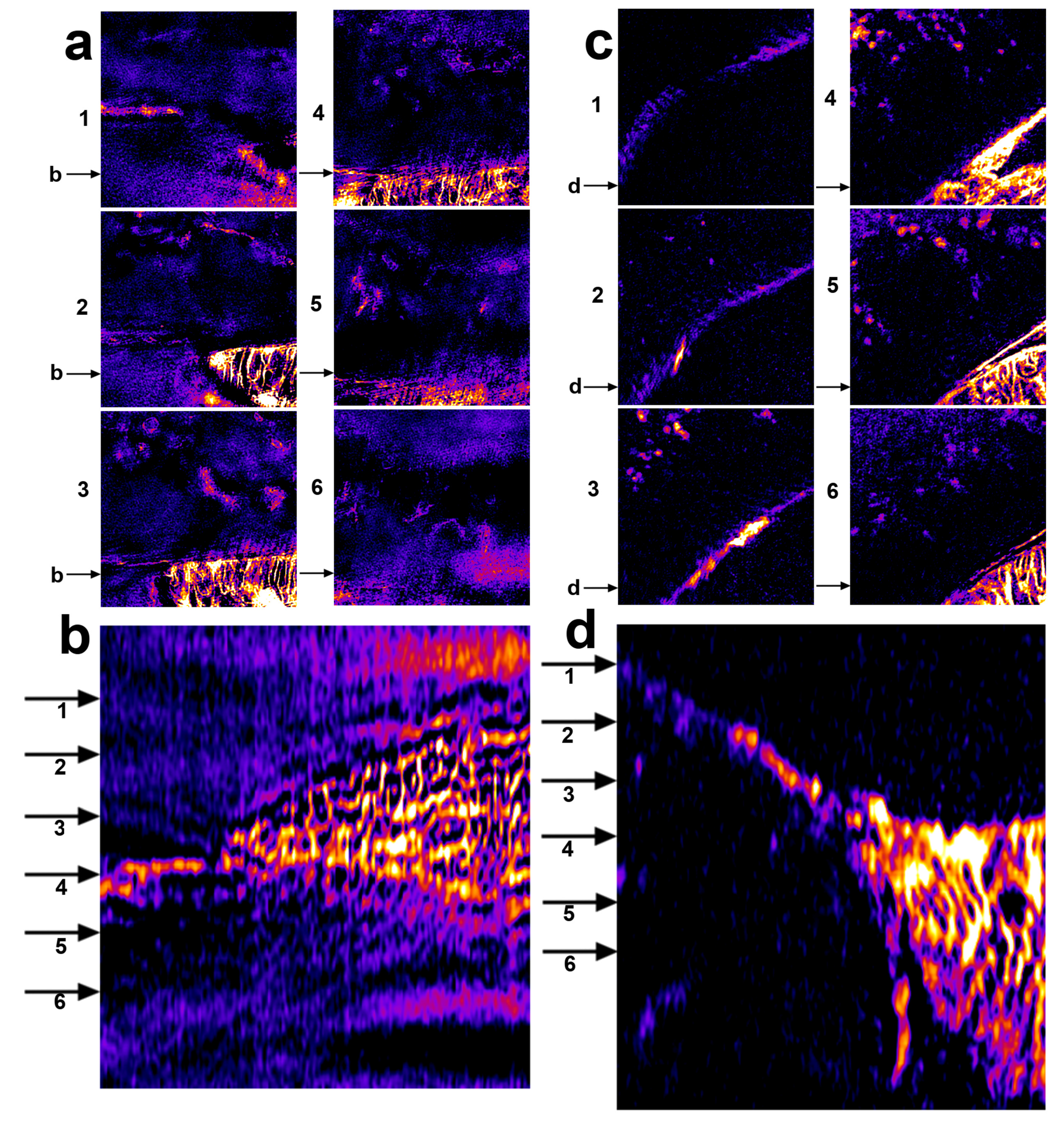
In order to allow a direct comparison of XL-SIM and ordinary line-grid 3D-SIM, we recorded stacks of the same mouse kidney sample as used in Figure 5, using a DeltaVision OMX Imaging System from GE Healthcare Life Sciences at the Center of Advanced Light Microscopy (CALM) of our university. A sample location of comparable thickness was chosen, showing features similar to our corresponding measurements. The left column in Figure 6 shows OMX images taken at selected planes (in a), and an section in b, whereas the right columns show corresponding images/sections acquired with our instrument. The chosen ROIs are 15 m × 15 m, the thickness of the SIM stack is approximately 15 m and the XL-SIM stack thickness amounts to approximately 17 m. The ROI shown in (c) and (d) is marked with `3’ in Figure 5a. The whole field of view for the ROI displayed in (a) and (b) is shown in Supplementary Figure S13.
One can clearly see how out-of-focus signal and noise degrade the image quality in the six focus layers of the SIM stack shown in Figure 6a, whereas the XL-SIM images in Figure 6c retain a similar image quality independant of sample-depth. One can hardly detect a difference to the performance obtained from much thinner sample (e.g., the tubulin sample shown in Figure 3. The slice in Figure 6b shows that an out-of-focus signal and noise in the SIM stack constitutes a kind of an echo from the in-focus signal, corresponding to the side lobes of the SIM axial response as shown in Figure 2d. In contrast, there’s virtually no out-of-focus echo in the slice shown in Figure 6d, consistent with the theoretically much smaller side lobes of the XL-SIM axial response shown in Figure 2d.
3. Discussion
We have shown that SIM using hexagonal patterns achieves the same resolution improvement as the conventional SIM approaches. However, XL-SIM offers the advantages of much simpler and more stable acquisition and processing of the 3D-SIM raw images, especially in the case of a thick biological specimen. Any errors in the determination of the pattern frequency vectors and z-positions, which can deteriorate the resolution and the homogeneity in the final processed SIM image, are minimized by using hexagonal patterns. The resolution abilities of XL-SIM were demonstrated qualitatively as well as quantitatively and a lateral resolution of approximately 106 has been verified. The axial resolution of the XL-SIM microscope has been shown to be approximately 297 . Both the lateral and axial resolution values double the resolution of the conventional optical microscope, which often makes a substantial difference in biological applications.
Furthermore, we have shown that XL-SIM also achieves better images from thicker and densely stained samples, e.g., from a 17 thick mouse kidney slice. In spite of contrast inhomogeneities, introduced by the interference of linear polarized diffraction orders, hexagonal SIM achieves the same resolution and S/N as standard SIM, but the usage of a hexagonal pattern essentially simplifies the raw image acquisition and offers an improved confocality. In principle, any (quasi-)confocal SIM microscope can be modified to become a super resolution SIM microscope, simply by changing the SIM substrate to a hexagonal phase pattern. In the case of 3D-SIM, only one (instead of three) stack(s) of raw images has to be recorded, which avoids any possible z-positioning errors, especially for large image stacks.
Furthermore, the SIM processing is simplified and accelerated by using hexagonal patterns because the frequency vectors of the SIM pattern can be calibrated before the measurement and don’t need to be changed and remeasured. The SIM pattern substrate has been mounted on a rotatable disc, whose rotation was only used to adjust the optimum orientation angle of the pattern relative to the shift direction. For future implementations of XL-SIM, we plan to introduce a linear stage for changing several SIM-patterns, e.g., for several excitation wavelengths.
In order to extend the working range of SIM-based super resolution to thicker samples(3D-)SIM, we combined (3D-)SIM with line-confocal excitation and detection. This was achieved by creating a line-shaped, hexagonally modulated excitation laser line, whose movement was synchronized with the movement of the rolling shutter of the sCMOS camera. The resulting line-confocality reduces the amount of out-of-focus light in the raw SIM phase-images, thus increasing their image contrast and hence the S/N of the resulting SIM image. The benefit of this approach increases with increasing sample thicknesses.
While confocality could be improved by using a narrower excitation line focus, this would diminish the excitation pattern contrasts (see also Figure 2a). To compensate for this, one could choose a smaller pattern base frequency, but that, in turn, would reduce the achievable SIM resolution. Thus, for thicker samples, a trade-off between resolution and confocality has to be made.
4. Materials and Methods
4.1. Fluorescence Excitation
An iBeam-Smart-488-S laser from the company TOPTICA (Gräfelfing, Germany) with a maximum output power of 200 mW has been used for excitation. A model/scheme of the excitation beam path is shown in Figure 1. The laser is shaped into a line by a custom Powell mirror (LT-Ultra, Herdwangen-Schönach, Germany). The line is scanned by a galvanometric scan mirror 6210H (Cambridge Technology, Bedford, MA, USA) across the field of view. A custom scan lens with mm (Sill Optics GmbH, S4LFT4345, Wendelstein, Germany) was used to focus the line onto the phase mask in the intermediate image. The galvanometers are driven by digital DC900 controller (SmartMove, Cambridge Technology). The back trace is faster than ms. A micro controller employing an embedded Linux system was used for the synchronization between the movement of the laser line and the rolling shutter window of the camera. The illumination pattern image is shifted by the rotation of a 5 mm glass window (Thorlabs WG11050-A, Newton, NJ, USA) mounted on a 6220H galvanometer (Cambridge Technology) behind the phase mask. A glass rotation of shifts the pattern by ≈30 m within 1 ms. There is no significant optical error up to a rotation of . The excitation tube lens was a mm lens from Zeiss (425308) (Oberkochen, Germany).The phase shift unit is a shaped Thorlabs WG11050-A on a CTI 6220H galvanometer.
4.2. Microscope Platform
The microscope platform is a novel microscope prototype from the company TILL I.D. (Planegg/Martinsried, Germany) A 3D model of the platform is shown in Supplementary Figure S2.
A Zeiss plan apochromat NA1.4 oil DIC was used as objective, which is designed for infinity space and a coverslip thickness of 170 . The objective was used in combination with ImmersolTM 518F/ISO8036 immersion oil ( (), ).
We used a filter set from the company Alluxa (Santa Rosa, CA, USA) consisting of a dichroic, an excitation and an emission filter suitable for a fluorescence excitation at 488 . The binary phase pattern has been designed as described in Supplementary Note 5 and was manufactured by the company Collischon Optik-Design in Erlangen, Germany. We chose the pattern period in the sample to be approximately twice the objective’s minimum resolvable distance. For the given objective, this corresponds to a period of 400 .
A user-defined tube lens (denoted as tube lense 2 in Figure 1 with a focal length of mm has been designed using the software ZEMAX. In combination with the objective, we have a total magnification factor of approximately 77×−78×.
A pco.edge 4.2 rolling shutter camera with a minimum acquisition time of 10 was used for the detection of the emission signal. By synchronization of the excitation scanning line movement with the movement of the rolling shutter active pixel area, we realized a slit confocal excitation and detection. The pixel pitch is 6.5 . We used the stage micrometer R1L3S2P (Thorlabs) for determination of pixel sizes in the sample and obtained a value of 84 .
The camera has two modes with different line times, which correspond to two different exposure times. Choosing a chip window of pixels and a rolling shutter height of 10 pixels corresponds to an exposure time of 100 with the fast mode. In some measurements, we used the slow mode, for which a rolling shutter height of 10 pixels corresponds to an exposure time of 275 . Exposure times below 550 can be realized by shifting the pattern times. An exposure time of 550 can, e.g., be realized by shifting the pattern 19 times and recording two phase images for every pattern position. This strategy avoids the shifts to become too small and the relative shift errors to become too large. If the 19 pattern shifts are carried out two times successively, two versions of each frequency band can be calculated. This allows for correcting thermal drift between the successive acquisitions analogously to [21].
4.3. Data Processing
The recorded raw image volumes have been processed with the software MATLAB (MATLAB R2013a, The MathWorks Inc., Natick, MA, USA).
4.4. Microscopic Samples
4.4.1. Nanorulers
Gatta-SIM nanorulers [37] (Gattaquant, Braunschweig, Germany) have been used in order to test and quantify the resolution of XL-SIM. Those nanorulers have two distinct fluorescent marks consisting of Alexa488 with a fixed distance of 120 .
4.4.2. Fluorescent Microspheres
We used green fluorescent aqueous microspheres with a diameter of 50 nm in order to test and characterize the resolution of XL-SIM (Thermo Fisher Scientific G50, Waltham, MA, USA). A cover slip (Zeiss ) was coated with polylysin, washed and dried. A drop of a diluted microsphere suspension was applied onto the coated coverslip. After some minutes, the surface was washed with water and dried. Then, the sample was sealed to a slide with UV-adhesive NOA63. The contact time of uncured adhesive and the microspheres has to be minimized.
4.4.3. Tubulin Sample
As previously described [38], mouse c2c12 cells were fixed for 10 min with 2% formaldehyde and subsequently washed three times with phosphate buffered saline (PBS). Cells were premeabilized for 10 min with 0.5% Triton X-100 diluted in PBS. After two washing steps with PBS plus 0.02% Tween (PBST) unspecific binding was blocked by incubation of the sample for 1 h with 2% BSA diluted in PBST. Tubulin was immunolabeled with a mouse anti tubulin monoclonal antibody (1:200) and after four washing steps (PBST) stained with a Alexa Fluor 488 conjugated secondary antibody (goat anti mouse 1:500). After four washing steps (PBST), cells were postfixed (4% formaldehyde), washed four times (PBST), and embedded in Vectashild fluid and surrounded by nail polish.
4.4.4. Mouse Kidney Sample
The mouse kidney sample was the FluoCells® prepared slide #3 from Thermo Fisher Scientific (Waltham, MA, USA), which is stained with Alexa Fluor® 488 WGA, Alexa Fluor® 568 Phalloidin, and DAPI. The average sample thickness is approximately 16 , and the maximum thickness is approximately 20 .
4.4.5. Thin Fluorescent Layers
The thin fluorescence layers that have been used for the orientation adjustment of the hexagonal pattern have been produced by spin coating: 2 ml PMMA in were mixed with 40 L mol/L Perylen-diimid-solution in . A single drop of approximately 8 were deposited on an with 2000 rpm rotating coverslip (Zeiss ). The sample has been sealed to the slide with the UV-adhesive NOA63.
4.5. Adjustment of Shift Angles and Calibration
The SIM pattern substrate has been mounted on a rotatable disc. The shift angles of the hexagonal pattern intensity in the sample have been adjusted by varying the orientation of the disc relative to the pattern shift direction. The orientation alignment procedure as well as the calibration of the shift widths are described in detail in Supplementary Note 1.
4.6. Parameter Fitting in SIM Processing
The parameters and are determined by complex linear regression of against using the before calibrated values of [21]. Explicitly, the parameter is evaluated by
where is the set of frequencies within the overlap of the nth frequency band with the 0th frequency band . Each information component is multiplied with its phase factor before evaluation of Equation (2). Analogously to the image processing described in [21], each information component has been multiplied by a filter function :
before shifting them in frequency space.
5. Conclusions
We have demonstrated that SIM, using a hexagonal pattern (X-SIM), achieves the same resolution enhancement as line-grid-SIM, but image acquisition and processing is simplified and become more stable – particularly for thicker samples – which require acquisition of extended z-stacks. These need to be recorded once only, instead of three times, as in conventional line-grid SIM. Another advantage is that pattern frequency vectors can be calibrated prior to the experiment.
By combining X-SIM with a line-confocal approach (XL-SIM), we were able to extend the working range of 3D-SIM into deeper layers, which line-grid SIM cannot reach because of the rapid drop in contrast when the whole field of view is excited and measured at once. Slit-confocality is achieved by scanning a hexagonally structured slit over the sample and synchronizing the rolling shutter window of a sCMOS cameras such that it acts as (slit-)confocal pinhole.
XL-SIM works equally well as a fast quasiconfocal sectioning tool and—simply by changing the pattern substrate—as super resolution instrument.
Supplementary Materials
Supplementary materials are available at: https://www.mdpi.com/2304-6732/4/2/33.
Acknowledgments
We want to thank Hartmann Harz and Andreas Maiser from the working group of Heinrich Leonhardt (Ludwig-Maximilians-Universität München, Department of Biology II, Grosshaderner Strasse 2, Martinsried D-82152, Germany) for making measurements at the OMX microscope for comparison with XL-SIM.
Author Contributions
M.S., R.U., and C.S. designed the instrument, M.S. and C.S. performed the experiments; M.S. analyzed data; and M.S., C.S., and R.U. wrote the paper.
Conflicts of Interest
The authors declare no conflict of interest.
Abbreviations
The following abbreviations are used in this manuscript:
| sCMOS | scientific Complementary metal-oxide-semiconductor |
| OTF | optical transfer function |
| PSF | point spread function |
| WF | Wide Field (Microscopy) |
| SIM | Structured Illumination Microscopy |
| L-SIM | Lineconfocal SIM |
| X-SIM | Hexagonal SIM |
| XL-SIM | Hexagonal Lineconfocal SIM |
| S/N | Signal-to-noise Ratio |
| LC | Line-confocal |
| FRC | Fourier Ring Correlation |
| DAPI | -Diamidin-2-phenylindol |
| WGA | Wheat Germ Agglutinin |
| PALM | Photoactivated Localization Microscopy |
| STORM | Stochastic Optical Reconstruction Microscopy |
| STED | Stimulated Emission Depletion |
References
- Conchello, J.A.; Lichtman, J.W. Optical sectioning microscopy. Nat. Methods 2005, 2, 920–931. [Google Scholar] [CrossRef] [PubMed]
- Neil, M.A.; Juskaitis, R.; Wilson, T. Method of obtaining optical sectioning by using structured light in a conventional microscope. Opt. Lett. 1997, 22, 1905–1907. [Google Scholar] [CrossRef] [PubMed]
- Neil, M.A.; Squire, A.; Juskaitis, R.; Bastiaens, P.I.; Wilson, T. Wide-field optically sectioning fluorescence microscopy with laser illumination. J. Microsc. 2000, 197, 1–4. [Google Scholar] [CrossRef] [PubMed]
- Brakenhoff, G.J.; Wurpel, G.W.H.; Jalink, K.; Oomen, L.; Brocks, L.; Zwier, J.M. Characterization of sectioning fluorescence microscopy with thin uniform fluorescent layers: Sectioned Imaging Property or SIPcharts. J. Microsc. 2004, 219, 122–132. [Google Scholar] [CrossRef] [PubMed]
- Weigel, A. Quantitation Strategies in Optically Sectioning Fluorescence Microscopy. Ph.D. Thesis, Fakultät für Biologie, Georg August Universität Göttingen, Göttingen, Germany, 2008. [Google Scholar]
- Wilson, T. Optical sectioning in fluorescence microscopy. J. Microsc. 2011, 242, 111–116. [Google Scholar] [CrossRef] [PubMed]
- Lukosz, W.; Marchand, M. Optischen Abbildung unter Überschreitung der Beugungsbedingten Auflösungsgrenze. Opt. Acta Int. J. Opt. 1963, 10, 241–255. [Google Scholar] [CrossRef]
- Lukosz, W. Optical Systems with Resolving Powers Exceeding the Classical Limit. J. Opt. Soc. Am. 1966, 56, 1463–1472. [Google Scholar] [CrossRef]
- Heintzmann, R.; Cremer, C. Laterally modulated excitation microscopy: Improvement of resolution by using a diffraction grating. Proc. SPIE 1999, 3568. [Google Scholar] [CrossRef]
- Gustafsson, M.G. Surpassing the lateral resolution limit by a factor of two using structured illumination microscopy. J. Microsc. 2000, 198, 82–87. [Google Scholar] [CrossRef] [PubMed]
- Betzig, E.; Patterson, G.H.; Sougrat, R.; Lindwasser, O.W.; Olenych, S.; Bonifacino, J.S.; Davidson, M.W.; Lippincott-schwartz, J.; Hess, H.F. Imaging Intracellular Fluorescent Proteins at Nanometer Resolution. Science 2006, 313, 1642–1645. [Google Scholar] [CrossRef] [PubMed]
- Rust, M.J.; Bates, M.; Zhuang, X. Sub-diffraction-limit imaging by stochastic optical reconstruction microscopy (STORM). Nat. Methods 2006, 3, 793–795. [Google Scholar] [CrossRef] [PubMed]
- Hell, S.W. Toward fluorescence nanoscopy. Nat. Biotechnol. 2003, 21, 1347–1355. [Google Scholar] [CrossRef] [PubMed]
- Li, D.; Shao, L.; Chen, B.C.; Zhang, X.; Zhang, M.; Moses, B.; Milkie, D.E.; Beach, J.R.; Hammer, J.A.I.; Pasham, M.; et al. Extended-resolution structured illumination imaging of endocytic and cytoskeletal dynamics. Science 2015, 349, 944–955. [Google Scholar] [CrossRef] [PubMed]
- Shao, L.; Kner, P.; Rego, E.H.; Gustafsson, M.G.L. Super-resolution 3D microscopy of live whole cells using structured illumination. Nat. Methods 2011, 8, 1044–1046. [Google Scholar] [CrossRef] [PubMed]
- Li, D.; Betzig, E. Response to Comment on “Extended-resolution structured illumination imaging of endocytic and cytoskeletal dynamics”. Science 2016, 352, 527. [Google Scholar] [CrossRef] [PubMed]
- Kner, P.; Chhun, B.B.; Griffis, E.R.; Winoto, L.; Gustafsson, M.G.L. Super-resolution video microscopy of live cells by structured illumination. Nat. Methods 2009, 6, 339–342. [Google Scholar] [CrossRef] [PubMed]
- Hagen, N.; Gao, L.; Tkaczyk, T.S. Quantitative sectioning and noise analysis for structured illumination microscopy. Opt. Express 2012, 20, 403–413. [Google Scholar] [CrossRef] [PubMed]
- Haase, S. OMX-A Novel High Speed and High Resolution Microscope and its Application to Nuclear and Chromosomal Structure Analysis. Ph.D. Thesis, Humboldt-Universitat zu Berlin, Berlin, Germany, 2007. [Google Scholar]
- Gustafsson, M.G.L.; Agard, D.A.; Sedat, J.W. Doubling the lateral resolution of wide-field fluorescence microscopy using structured illumination. Proc. SPIE 2000, 3919, 141–150. [Google Scholar]
- Gustafsson, M.G.L.; Shao, L.; Carlton, P.M.; Wang, C.J.R.; Golubovskaya, I.N.; Cande, W.Z.; Agard, D.A.; Sedat, J.W. Three-Dimensional Resolution Doubling in Wide-Field Fluorescence Microscopy by Structured Illumination. Biophys. J. 2008, 94, 4957–4970. [Google Scholar] [CrossRef] [PubMed]
- Mandula, O.; Kielhorn, M.; Wicker, K.; Krampert, G.; Kleppe, I.; Heintzmann, R. Line scan–structured illumination microscopy super-resolution imaging in thick fluorescent samples. Opt. Express 2012, 20, 24167–24174. [Google Scholar] [CrossRef] [PubMed]
- Schropp, M.; Uhl, R. Two-dimensional structured illumination microscopy. J. Microsc. 2014, 256, 23–36. [Google Scholar] [CrossRef] [PubMed]
- Frohn, J.T. Super-Resolution Fluorescence Microscopy by Structured Light Illumination. Ph.D. Thesis, Swiss Federal Institute of Technology Zurich, Zürich, Switzerland, 2000. [Google Scholar]
- Heintzmann, R. Saturated patterned excitation microscopy with two-dimensional excitation patterns. Micron 2003, 34, 283–291. [Google Scholar] [CrossRef]
- O’Holleran, K.; Shaw, M. Polarization effects on contrast in structured illumination microscopy. Opt. Lett. 2012, 37, 4603–4605. [Google Scholar] [CrossRef] [PubMed]
- Shroff, S.A.; Fienup, J.R.; Williams, D.R. OTF compensation in structured illumination super resolution images. Proc. SPIE 2008, 7094. [Google Scholar] [CrossRef]
- Heintzmann, R. Structured Illumination Methods. In Handbook of Confocal Microscopy; Springer Science + Business Media, LLC: New York, NY, USA, 2006; Chapter 13; pp. 265–279. [Google Scholar]
- Righolt, C.H.; Slotman, J.A.; Young, I.T.; Vliet, L.J.V.; Stallinga, S. Image filtering in structured illumination microscopy using the Lukosz bound. Opt. Express 2013, 21, 1599–1609. [Google Scholar] [CrossRef] [PubMed]
- Saxton, W.; Baumeister, W. The correlation averaging of a regularly arranged bacterial cell envelope protein. J. Microsc. 1982, 127, 127–138. [Google Scholar] [CrossRef] [PubMed]
- Bui, K.H.; Lemke, E.A.; Beck, M. Fourier ring correlation as a resolution criterion for super-resolution microscopy. J. Struct. Biol. 2013, 183, 363–367. [Google Scholar]
- Nieuwenhuizen, R.P.J.; Lidke, K.A.; Bates, M.; Puig, D.L.; Stallinga, S.; Rieger, B. Measuring image resolution in optical nanoscopy. Nat. Methods 2013, 10, 557–562. [Google Scholar] [CrossRef] [PubMed]
- Agard, D.A.; Hiraoka, Y.; Shaw, P.; Sedat, J.W. Fluorescence microscopy in three dimensions. Methods Cell Biol. 1989, 30, 353–377. [Google Scholar] [PubMed]
- Schermelleh, L.; Carlton, P.M.; Haase, S.; Shao, L.; Winoto, L.; Kner, P.; Burke, B.; Cardoso, M.C.; Agard, D.A.; Gustafsson, M.G.L.; et al. Subdiffraction Multicolor Imaging of the Nuclear Periphery with 3D Structured Illumination Microscopy. Science 2008, 320, 1332–1336. [Google Scholar] [CrossRef] [PubMed]
- Carrington, W.; Lynch, R.; Moore, E.; Isenberg, G.; Fogarty, K.E.; Fay, F. Super-resolution three-dimensional images of fluorescence in cells with minimal light exposure. Science 1995, 268, 1483–1487. [Google Scholar] [CrossRef] [PubMed]
- Chakrova, N.; Rieger, B.; Stallinga, S. Deconvolution methods for structured illumination microscopy. J. Opt. Soc. Am. 2016, 33, 12–20. [Google Scholar] [CrossRef] [PubMed]
- Schmied, J. Testing and Pushing the Limits of Super-Resolution Microscopy. Opt. & Photonik 2016, 11, 23–26. [Google Scholar]
- Smeets, D.; Markaki, Y.; Schmid, V.J.; Kraus, F.; Tattermusch, A.; Cerase, A.; Sterr, M.; Fiedler, S.; Demmerle, J.; Popken, J.; et al. Three-dimensional super-resolution microscopy of the inactive X chromosome territory reveals a collapse of its active nuclear compartment harboring distinct Xist RNA foci. Epigenetics Chromatin. 2014, 7, 1–27. [Google Scholar] [CrossRef] [PubMed]
Figure 1.
Schematic drawing of the slit-confocal structured excitation: the excitation laser line is generated by a Powell lens and scanned over the structured illumination microscopy (SIM) mask with an galvanometric mirror (galvo). The SIM pattern substrate is imaged onto the sample by the excitation tube lens 1 and the microscope objective. Excitation and emission light is separated by dichroic filters (dichro) and the patterned excitation line image is shifted in the sample by the galvanometric phase shift unit. The sample is imaged onto the sCMOs camera by the microscope objective and the emission tube lens 2.

Figure 2.
Principle of excitation in XL-SIM. (a) (left): amplitude of the excitation in the microscope objective pupil. The seven first diffraction orders of the hexagonal pattern can pass the pupil, which is indicated by a circle. Note that the diffraction orders are broadened by the line shaped excitation. (right): corresponding spatial frequency spectrum of the integrated excitation intensity and the shift vector ; (b) (left): section of the excitation laser line for a given point in time. The line has a spatial extent of about three periods of the hexagonal pattern. (right): section of the laser line. Note that the white vertical line in the left image corresponds to the white horizontal line in the right image; (c) simulated excitation contrasts for SIM and XL-SIM as a function of defocus; (d) the axial response (confocality) for SIM and XL-SIM as a function of defocus illustrated as logarithmic plot.

Figure 3.
Demonstration of resolution improvement by XL-SIM: (a) line-confocal (LC) image of a tubulin sample. The field of view is ; A corresponding XL-SIM image is shown in (b); because the dynamic range of both images amounts approximately 10 bits, a colored lookup table (fire) has been used; Figures (c,d) or (e,f) show the regions of interest which are marked by `1’ or `2’, respectively. The arrows indicate sample features that are unresolved in the LC image but can clearly be recognized in the XL-SIM image; in contrast to (c), the lack of resolution in (e) is partially caused by detected out-of-focus light; and Figure (g) shows a line profile plot along the white lines in (c,d).
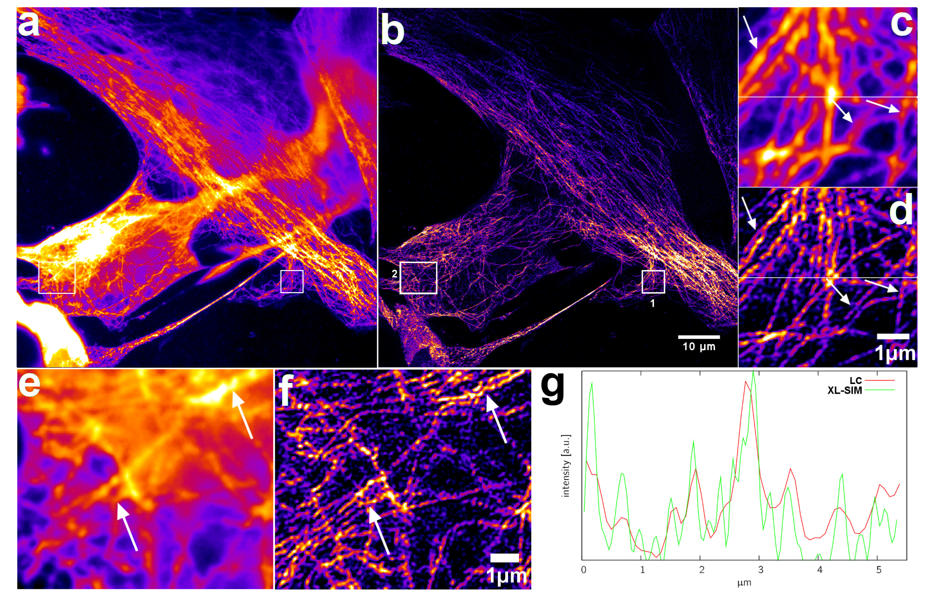
Figure 4.
Characterization of resolution improvement ability of XL-SIM: (a) Wide field (WF) image of nanorulers, which have a distance of 120 . The corresponding image for XL-SIM is shown in (b); in contrast to (a), the nanorulers in focus can clearly be distinguished in (b); a plot of a Fourier-ring correlation for an XL-SIM image with the commonly used threshold value of ≈0.143 is shown in (c); according to this threshold, our XL-SIM approach gives a resolution of approximately nm. A volume of green fluorescent microspheres with a diameter of nm has been recorded. An -view of line-confocal and XL-SIM ROIs of the volume are shown in (d,e); the arrows indicate several beads whose distance is to small to be distinguished in the WF image (d) but can be resolved in the XL-SIM image (e); the area between the white horizontal lines in (d,e) is maximum projected in the y-direction and shown as a view of the volume in (g,h). A Gaussian distribution has been fitted to the intensity distribution of 537 microspheres in and z. Corresponding lateral and axial full-width-at-half-maximum (FWHM) values are illustrated in (f).

Figure 5.
Example of 3D-XL-SIM with a mouse kidney section, labeled with Alexa Fluor® 488 WGA, Alexa Fluor® 568 Phalloidin, and DAPI and measured with an excitation of 488 nm. The measured volume has a total size of . The XL-SIM-image for the middle layer of the volume is shown in (a); the corresponding line-confocal image is shown in (d); the ROIs which are indicated with `1’ and `2’ are shown enlarged in figures (b,c) for the XL-SIM image and in (e,f) for the line-confocal image; Figure (g) shows orthogonal intensity profiles of the measured volume in 3D; and a 3D rendered object is shown in (h).
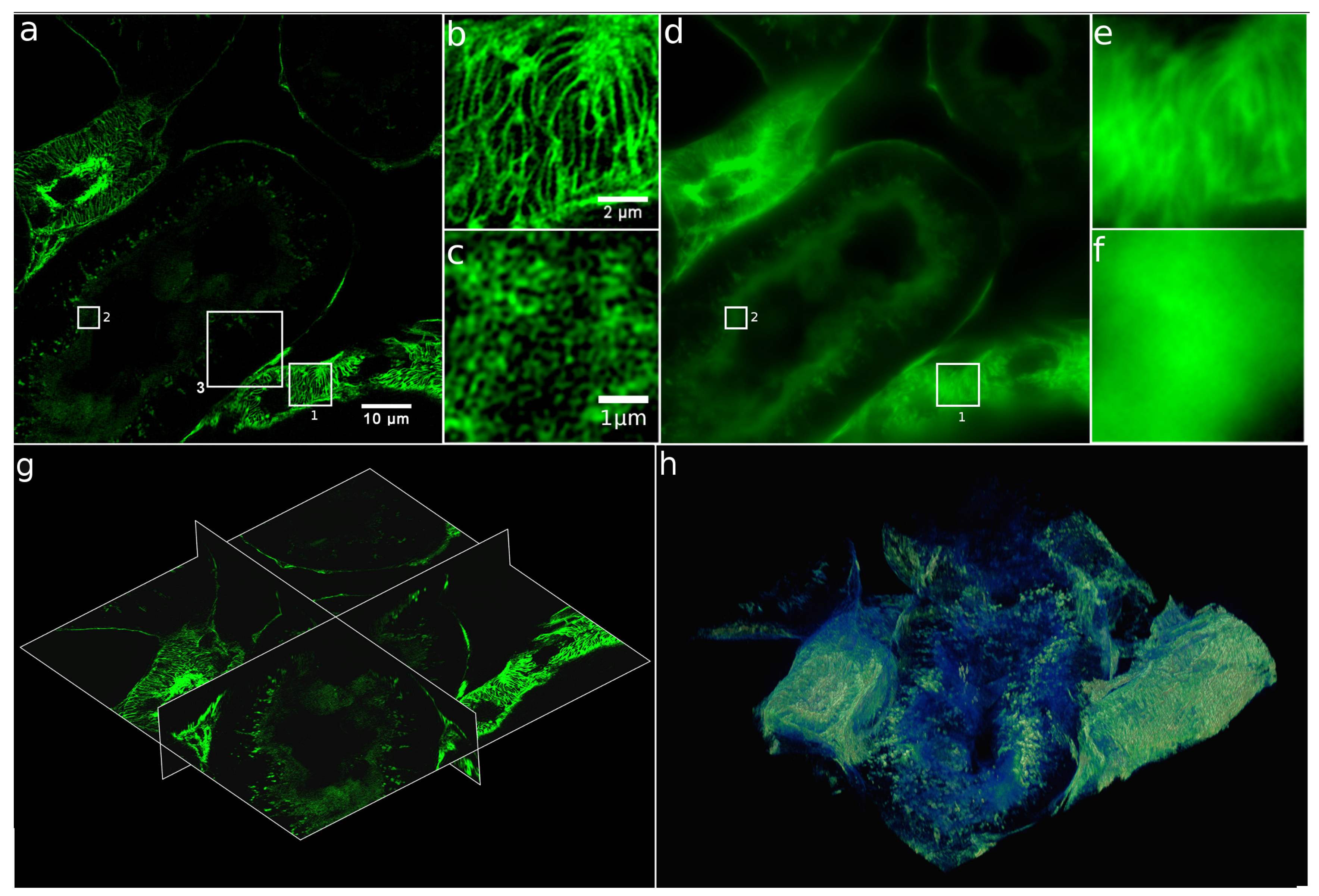
Figure 6.
Comparison of SIM with XL-SIM: (a) six different focus layers of the SIM image stack; (b) slice of the SIM image stack. The arrows in (a) mark the y-location of the slice in (b); the arrows in (b) mark the six different focus positions shown in (a); the corresponding measurements for XL-SIM are shown in (c,d); and the field of view in the images in (a) and (c) is 15 15 . The stack thickness is in the SIM measurement and in the XL-SIM measurement.

© 2017 by the authors. Licensee MDPI, Basel, Switzerland. This article is an open access article distributed under the terms and conditions of the Creative Commons Attribution (CC BY) license (http://creativecommons.org/licenses/by/4.0/).
Share and Cite
MDPI and ACS Style
Schropp, M.; Seebacher, C.; Uhl, R. XL-SIM: Extending Superresolution into Deeper Layers. Photonics 2017, 4, 33. https://doi.org/10.3390/photonics4020033
AMA Style
Schropp M, Seebacher C, Uhl R. XL-SIM: Extending Superresolution into Deeper Layers. Photonics. 2017; 4(2):33. https://doi.org/10.3390/photonics4020033
Chicago/Turabian StyleSchropp, Martin, Christian Seebacher, and Rainer Uhl. 2017. "XL-SIM: Extending Superresolution into Deeper Layers" Photonics 4, no. 2: 33. https://doi.org/10.3390/photonics4020033
Note that from the first issue of 2016, this journal uses article numbers instead of page numbers. See further details here.