Label-Free Saturated Structured Excitation Microscopy


1
Department of Chemistry and Biochemistry, Montana State University, Bozeman, MT 59717, USA
2
Montana Materials Science Program, Montana State University, Bozeman, MT 59717, USA
*
Author to whom correspondence should be addressed.
Photonics 2017, 4(2), 36; https://doi.org/10.3390/photonics4020036
Submission received: 14 March 2017
/
Revised: 17 April 2017
/
Accepted: 2 May 2017
/
Published: 5 May 2017
(This article belongs to the Special Issue Superresolution Optical Microscopy)
Abstract
:Micro- and nanoscale chemical and structural heterogeneities, whether they are intrinsic material properties like grain boundaries or intentionally encoded via nanoscale fabrication techniques, pose a challenge to current material characterization methods. To precisely interrogate the electronic structure of these complex materials systems, spectroscopic techniques with high spatial resolution are required. However, conventional optical microscopies are limited to probe volumes of ~200 nm due to the diffraction limit of visible light. While a variety of sub-diffraction-limited techniques have been developed, many rely on fluorescent contrast agents. Herein we describe label-free saturated structured excitation microscopy (LF-SSEM) applicable to nonlinear imaging approaches such as stimulated Raman and pump-probe microscopy. By exploiting the nonlinear sample response of saturated excitation, LF-SSEM provides theoretically limitless resolution enhancement without the need for a photoluminescent sample.
1. Introduction
The micro- to nanoscale heterogeneity of complex material systems complicates optical characterization due to the diffraction limit of light [1], which limits coherent spectroscopic techniques to probe volumes greater than ~200 nm. A variety of super-resolution far-field microscopies have been developed which surpass the diffraction limit [2,3,4,5,6]. These techniques, however, remain tied to fluorescent properties inherent to the material or to those introduced by fluorescent markers. In contrast, coherent super-resolution microscopies provide sub-diffraction-limited material characterization without the need for fluorescent markers [7,8,9,10]. Far-field coherent super-resolution techniques rely on principles first developed for fluorescence microscopies. For example, the principles of stimulated emission depletion [5] have been successfully applied to Stimulated Raman Microscopy (SRM) [7] and to Pump-Probe Microscopy (PPM) [8]. Our research group has leveraged the theoretical basis of Laterally Modulated Excitation Microscopy [6] to develop Structured PPM, which provides a factor of two improvement in spatial resolution without relying on high-intensity saturation or de-excitation phenomena [11,12]. To achieve higher imaging resolution with a structured excitation field, it is necessary to invoke higher order nonlinear light-matter interactions [13,14]. Herein, we describe the impact of saturated excitation on label-free coherent third-order nonlinear optical microscopy techniques including PPM and SRM. Label-free saturated structured excitation microscopy (LF-SSEM) exploits the nonlinear saturation of the excitation process in conjunction with a structured excitation field to collect high spatial frequency information that would otherwise not pass through the optical system. In doing so, LF-SSEM can theoretically provide unlimited spatial resolution. In the remainder of the paper, we describe the imaging theory of LF-SSEM and theoretically demonstrate a factor of six improvement in resolution over the diffraction limit, corresponding to a point spread function of ~33 nm with a 400-nm excitation wavelength.
2. Methods
2.1. Imaging Theory
In a scanning nonlinear optical microscope, image formation can be described by Equation (1):
where o(r) is the object function, E(r) is the electric field, and h(r) represents the point spread function (PSF) of the imaging system. Here, represents the convolution operation. A diffraction-limited (DL) image, generated via related third-order techniques like PPM or SRM, can be described by:
where the effective electric field () of Equation (1) has been recast to explicitly show the multiple interactions with the electric field in third-order techniques. The DL image () resolution is determined by the convolution of the object (o(r)) with the product of the squared excitation (E1(r)) and probe (E2(r)) electric fields, each separately convolved with its individual optical PSF (h1, h2). Experimentally, the spatial convolution of the object with the effective electric field is performed by focusing both DL beams at the sample plane and raster scanning the sample beneath them. The Fourier transform (FT) of Equation (2):
yields the conjugate space representation of the DL image. Here we use capital letters and tildes to denote conjugate-space terms. The DL spectrum () can be understood as the object spectrum () filtered by a triple convolution of the four optical transfer functions (OTFs; ). A detailed discussion of DL imaging theory can be found elsewhere [11,12].
2.2. Structured Excitation
Imaging with conventional nonlinear scanning microscopies utilizes point-focused excitation and probe beams at the sample plane. LF-SSEM replaces the DL excitation beam with a structured excitation field to collect additional high spatial frequency information that would otherwise be attenuated by the optical system. In the case of one dimensional structured excitation, the field E1 in Equation (2) is given by a sinusoidally modulated excitation profile:
where kx and φx give the period and phase, respectively, of the excitation field propagating along the x-axis. Replacing the DL excitation pulse of Equation (2) with the structured excitation field in Equation (4) results in the collection of a structured image ():
that is dependent on the period and phase of the excitation profile. The excitation pulse PSF is eliminated from Equation (5), due to the necessary condition that the spatial frequency of the excitation profile falls within the bounds of the optical transfer function of the imaging system. Under conditions where the excitation density scales linearly with the pump power (low fluence), a series of structured images collected with a structured excitation field like that given by Equation (4) can be utilized to reconstruct an image with a factor of two improvement in spatial resolution over the diffraction limit [11,12].
2.3. Saturated Excitation
To increase the resolution of structured excitation microscopy beyond a two-fold improvement, a nonlinear excitation process must be exploited. For intense pulsed lasers, saturated excitation can be expressed by Equation (6) [14]:
where E1(x) is the structured excitation field in Equation (4) and n is an effective scaling factor that determines the extent of nonlinearity in the excitation process. As shown in Panel A of Figure 1, linear excitation occurs for small values of n (n << 1), while for larger values of n, the excitation process becomes increasingly saturated. The black (circles), red (squares), green (triangles) and blue (diamonds) traces of Panel B in Figure 1 show the excitation profiles for increasing values of n. To account for the nonlinear excitation profile in the structured image, Equation (5) must be modified with the new field expression given by Equation (6).
The expansion of Equation (6) and truncation of the series after the fourth-order term gives:
where each term in square brackets is labeled with an index indicating the order of the light-matter interaction. Fourier transform of each of the four terms in Equation (8) produces frequency components located at increasing intervals of ±2kx in conjugate space. The first (linear) term is comprised of components at k = ±2kx (as well as at k = 0), while the second-order term has components at k = ±4kx (and ±2kx, 0), etc. By truncating the series at the fourth-order term, we limit our analysis to Fourier components up to k = ±8kx. Panel C of Figure 1 shows the Fourier components of the excitation field up to k = ±8kx for n = 1. In principle, the expansion can be limitless, and is only restricted by the relative amplitude of the higher order Fourier components with respect to the noise of the measurement [14]. In Panel D of Figure 1, we show the relative amplitude of the linear and nonlinear Fourier components as n is increased. While the nonlinear terms are weak relative to the linear terms, image formation that exploits higher order Fourier components will benefit from lock-in detection often utilized with third-order imaging techniques [15].
2.4. Image Reconstruction
As illustrated in Panel C of Figure 1, the saturation of the excitation process increases the number of Fourier components that contribute to image formation. The key to reconstructing an image with increased spatial resolution is to collect a series of images in which the phase of the excitation field is shifted by a known interval at the sample plane. Previous work has discussed the process of image reconstruction under linear excitation conditions [11,12]. Image reconstruction under nonlinear excitation conditions is entirely analogous to the linear case, with the exception that additional phase-shifted structured images must be collected to enable unique identification of the additional frequency components present in the collected images.
Once collected, the vector of m individual Fourier components, , are determined by solving the linear system given by:
Here, is the inverted m × m matrix of amplitude and phase information encoded by the excitation field, and is the m-length vector of conjugate space structured images [12]. Summing the m components of yields the total reconstructed conjugate space image.
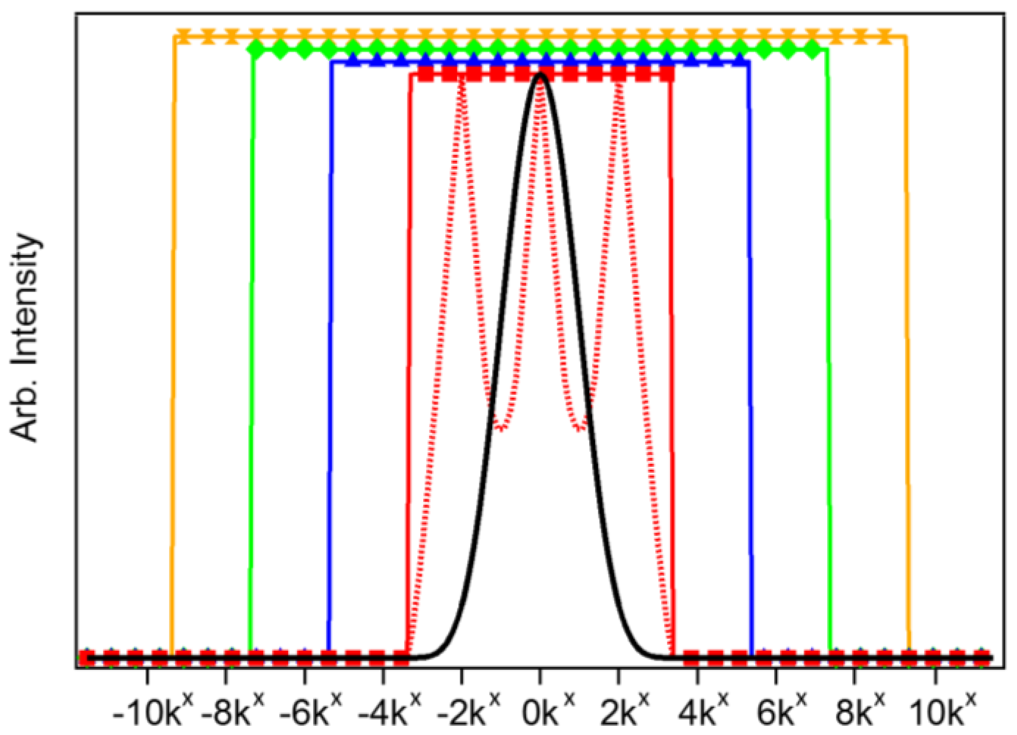
Figure 2 presents the effective LF-SSEM OTF when utilizing Fourier components up to k = ±2kx (red; squares), ±4kx (blue; triangles), ±6kx (green; diamonds), and ±8kx (yellow; hourglass). The red dashed trace shows the raw reconstructed linear regime OTF before amplitude normalization by the ideal OTF [12]. As the OTF effectively acts as a low-pass (spatial) frequency filter, expanding it through LF-SSEM provides access to higher spatial frequency information than that which is transmitted in the DL case (black trace).
3. Results
3.1. PSF Comparison
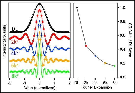
The improvement to the LF-SSEM PSF is summarized in Figure 3, where the DL and LF-SSEM images of a single point source are compared. The coordinate system was defined to be consistent with previously published results, corresponding to a 0.9 NA objective and pump/probe wavelength ratio of 0.87 [11]. Panel A of Figure 3 compares the PSFs of the LF-SSEM model (red squares; green circles) to the DL case (black dashed) with the full width at half maximum (FWHM) of the DL model normalized to 1. The PSF indicated by the red squares includes only the linear Fourier components (OTF defined by red squares in Figure 2), whereas the green circles indicate the resultant PSF if all Fourier components up to k = ±8kx are included (yellow OTF in Figure 2). Because the inclusion of higher order Fourier components in the construction of the image provides access to higher spatial frequency information in the conjugate image, the PSF is significantly narrower in the real-space image. Panel B summarizes this effect by plotting the FWHM of each PSF as increasingly higher order components are included in the image formation. The most significant reduction in width occurs after the inclusion of the linear components at k = ±2kx, however, if all components up to the fourth-order term are included, the PSF can be reduced in width by more than a factor of six. As a best-case scenario with λexcitation = 400 nm and λprobe = 400 nm, these results indicate that the PSF will have a width of only 33.4 nm. The LF-SSEM PSFs shown in Panel A of Figure 3 exhibit ringing outward from the center peak. The oscillatory ringing results from the Fourier transform of the sharp-edged OTF functions are shown in Figure 2. By smoothing the high-frequency edges of the OTF, the ringing can be mitigated, although at the cost of a wider PSF.
3.2. Imaging Capabilities
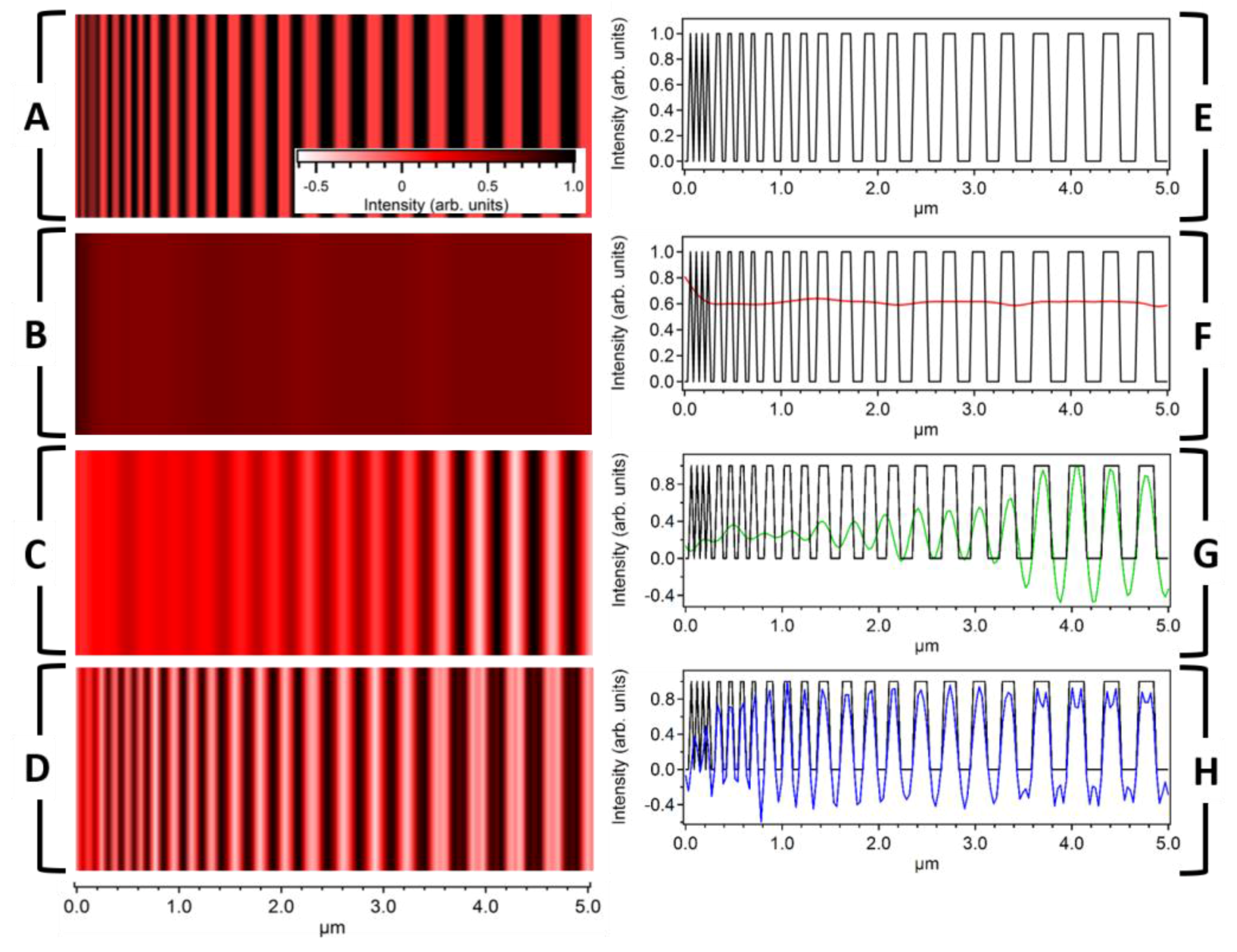
We next modeled the imaging capabilities of LF-SSEM using a simulated grating structure with line widths decreasing from 180 nm to 30 nm. The excitation and probe wavelengths were 784 nm and 900 nm, respectively, corresponding to a DL PSF FWHM of 432.2 nm. Panel A of Figure 4 shows the simulated target and Panel B shows the image produced by the DL model. The LF-SSEM images in Panel C, which includes Fourier components up to k = ±2kx, and Panel D, which includes Fourier components up to k = ±8kx, have significantly improved resolutions relative to the DL case. The enhanced resolution can be seen more clearly in Panels F, G, and H, where the profiles of the images are compared. For the DL case (Panel F; red), even the largest features of the target image (black) remain unresolved. On the other hand, LF-SSEM models (Panel G and H) resolve components spaced far below the diffraction limit. If Fourier components up to the fourth-order are included (Panel H), LF-SSEM resolves features spaced only 60.2 nm apart, representing an approximate factor of six improvement in spatial resolution. Two artifacts of the LF-SSEM approach, both a consequence of the PSF ringing discussed above, can be seen in Panel H. The first is a negative offset that spans the image from approximately 0.5–5 μm. This offset arises from the negative amplitude ringing in the PSF (see Figure 3A), which constructively interferes for two neighboring object features. The second artifact takes the form of the low-amplitude peaks near 4.0 μm. Again, these peaks can be understood as interference of the neighboring grating features after convolution with the LF-SSEM PSF. In this case, because the relative spacing of the object features is larger, the ringing interferes differently, manifesting in the small specious peaks.
While we have modeled LF-SSEM in one dimension, multi-dimensional resolution enhancement can be approached in two ways. First, as has been demonstrated [14] in fluorescence imaging, full radial super-resolution can be achieved by collecting patterned images with a one-dimensional excitation pattern, rotated through a series of angles around the axis normal to the sample plane. Rotating the image in such a manner is straightforward using modern pulse shaping technologies such as spatial light modulators or digital micromirror devices. The second approach requires a two-dimensional structured excitation profile, which resembles a two-dimensional diffraction pattern [13]. While no pattern rotation is necessary in this case, each Fourier component must be isolated with a unique phase, a requirement that introduces additional experimental and image-processing difficulties. To provide perspective as to how rapidly the number of required images increases with increasing dimensionality and saturation, we assume the use of a sequential one-dimensional structured excitation performed using pattern rotation steps of π/6 to reach full radial resolution enhancement. In order to produce a two-fold resolution in the linear excitation regime, 18 images would be needed to solve the system of linear equations during reconstruction. To produce a four-fold increase in resolution (corresponding to the nonlinear expansion of Fourier components up to ±6kx), 42 images would be required. Note that the number of images described above can be reduced by approximately a factor of two as the Fourier components shifted to opposite signs (i.e., ±6kx) contain redundant information (i.e., they are complex conjugates of one another), however, the imaging process is still experimentally demanding.
3.3. Signal-to-Noise Ratio Dependence
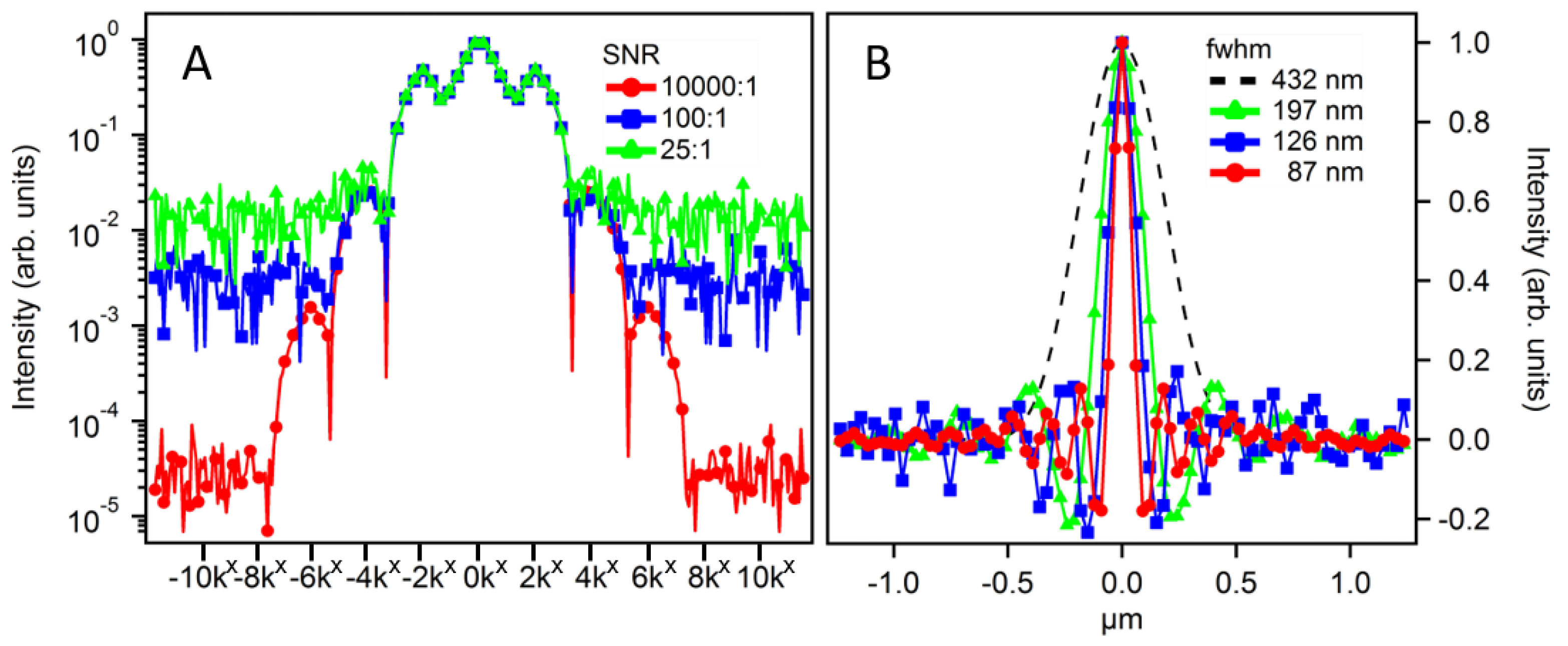
Thus far, we have modeled the LF-SSEM approach assuming an ideal imaging system to produce resolution enhancement without regard to noise present in experimental applications. In the case of negligible levels of noise, LF-SSEM provides theoretically limitless resolution. However, in practice, noise will prevent isolation of the low-amplitude, higher order Fourier components. In Figure 5 we show modeled results of the imaging process while including random noise with a uniform probability distribution. Panel A shows a profile comparison of the structured image spectrum at varying signal-to-noise ratios (SNRs). Excitation fluence was held constant at a level capable of producing a Fourier expansion up to ±6kx. When the SNR is high (10,000:1), all seven Fourier components rise above the noise level. However, when the SNR is low (100:1 and 25:1), fewer Fourier components are distinguishable above the noise threshold. Panel B shows the profile comparison of the PSFs resulting from the corresponding SNR of Panel A. If the higher order Fourier component has a negligible amplitude relative to the noise level, the OTF expansion is limited during image reconstruction. At an SNR of 10,000:1 the OTF was expanded to ±6kx, while SNRs of 100:1 and 25:1 only allowed for the OTF expansion of ±4kx and ±2kx, respectively. In practice, both the high order Fourier component amplitudes and the SNR can be increased by increasing the pump fluence, provided the sample is robust to high excitation levels.
4. Conclusions
We have demonstrated the resolution enhancement of LF-SSEM when the saturation of the excitation process allows for the collection of higher order nonlinear spatial frequency components. Our results suggest that PSFs as narrow as ~33 nm can be achieved if Fourier components up to the fourth-order are included in the image formation. However, LF-SSEM is capable of achieving even greater resolution enhancement provided the optical configuration has a low noise threshold. The approach outlined for LF-SSEM can be readily applied to related nonlinear imaging techniques such as SRM and PPM, which share a common electric field and phase-matching dependence. Further advancements of LF-SSEM will seek to demonstrate experimental viability and determine which multidimensional approach is experimentally preferable. We expect that with further advancement, LF-SSEM and related far-field super-resolution microscopies can become viable alternatives to near-field characterization techniques for nanoscale materials systems.
Acknowledgments
This work was funded by the Division of Chemical Sciences, Geosciences, and Biosciences, Office of Basic Energy Sciences of the U.S. Department of Energy through Grant DE-SC0014128.
Author Contributions
E.G. conceived the experiment. E.M. performed the modeling and analyzed the results. E.M. and E.G. wrote the paper.
Conflicts of Interest
The authors declare no conflict of interests. The funding sponsors had no role in the design of the study; in the collection, analyses, or interpretation of data; in the writing of the manuscript, and in the decision to publish the results.
References
- Köhler, H. On abbe’s theory of image formation in the microscope. Opt. Acta Int. J. Opt. 1981, 28, 1691–1701. [Google Scholar] [CrossRef]
- Schermelleh, L.; Heintzmann, R.; Leonhardt, H. A guide to super-resolution fluorescence microscopy. J. Cell Biol. 2010, 190, 165–175. [Google Scholar] [CrossRef] [PubMed]
- Rust, M.J.; Bates, M.; Zhuang, X. Sub-diffraction-limit imaging by stochastic optical reconstruction microscopy (storm). Nat. Methods 2006, 3, 793–795. [Google Scholar] [CrossRef] [PubMed]
- Betzig, E.; Patterson, G.H.; Sougrat, R.; Lindwasser, O.W.; Olenych, S.; Bonifacino, J.S.; Michael, W.; Davidson, J.L.-S.; Hess, H.F. Imaging intracellular fluorescent proteins at nanometer resolution. Science 2006, 313, 1642–1645. [Google Scholar] [CrossRef] [PubMed]
- Hell, S.W.; Wichmann, J. Breaking the diffraction resolution limit by stimulated emission- stimulated-emission-depletion fluorescence microscopy. Opt. Lett. 1994, 19, 780–782. [Google Scholar] [CrossRef] [PubMed]
- Heintzmann, R.; Cremer, C. Laterally modulated excitation microscopy—Improvement of resolution by using a diffraction grating. Proc. SPIE 1999, 3568, 185–196. [Google Scholar]
- Silva, W.R.; Graefe, C.T.; Frontiera, R.R. Toward label-free super-resolution microscopy. ACS Photonics 2016, 3, 79–86. [Google Scholar] [CrossRef]
- Wang, P.; Slipchenko, M.N.; Mitchell, J.; Yang, C.; Potma, E.O.; Xu, X.; Cheng, J.X. Far-field imaging of non-fluorescent species with sub-diffraction resolution. Nat. Photonics 2013, 7, 449–453. [Google Scholar] [CrossRef] [PubMed]
- Liu, N.; Kumbham, M.; Pita, I.; Guo, Y.; Bianchini, P.; Diaspro, A.; Tofail, S.A.M.; Peremans, A.; Silien, C. Far-field subdiffraction imaging of semiconductors using nonlinear transient absorption differential microscopy. ACS Photonics 2016, 3, 478–485. [Google Scholar] [CrossRef]
- Hajek, K.M.; Littleton, B.; Turk, D.; McIntyre, T.J.; Rubinsztein-Dunlop, H. A method for achieving super-resolved widefield cars microscopy. Opt. Express 2010, 18, 19263–19272. [Google Scholar] [CrossRef] [PubMed]
- Massaro, E.S.; Hill, A.H.; Grumstrup, E.M. Super-resolution structured pump–probe microscopy. ACS Photonics 2016, 3, 501–506. [Google Scholar] [CrossRef]
- Massaro, E.S.; Hill, A.H.; Kennedy, C.L.; Grumstrup, E.M. Imaging theory of structured pump-probe microscopy. Opt. Express 2016, 24, 20868–20880. [Google Scholar] [CrossRef] [PubMed]
- Heintzmann, R. Saturated patterned excitation microscopy with two-dimensional excitation patterns. Micron 2003, 34, 283–291. [Google Scholar] [CrossRef]
- Gustafsson, M.G. Nonlinear structured-illumination microscopy: Wide-field fluorescence imaging with theoretically unlimited resolution. Proc. Nat. Acad. Sci. USA 2005, 102, 13081–13086. [Google Scholar] [CrossRef] [PubMed]
- Frolov, S.V.; Vardeny, Z.V. Double-modulation electro-optic sampling for pump-and-probe ultrafast correlation measurements. Rev. Sci. Instrum. 1998, 69, 1257–1260. [Google Scholar] [CrossRef]
Figure 1.
Label-free saturated structured excitation microscopy (LF-SSEM) saturation effects. (A) Nonlinear relationship of the excitation fluence (n) and saturation of the excitation process. (B) Effective excitation density at the sample plane as the extent of saturation is increased. (C) Normalized relative amplitude of nine Fourier components produced from an excitation profile given by the black (circle) trace in Panel B. (D) Relationship of Fourier component amplitude and effective excitation fluence. The colors and markers of Panel D correspond to the components of Panel C.
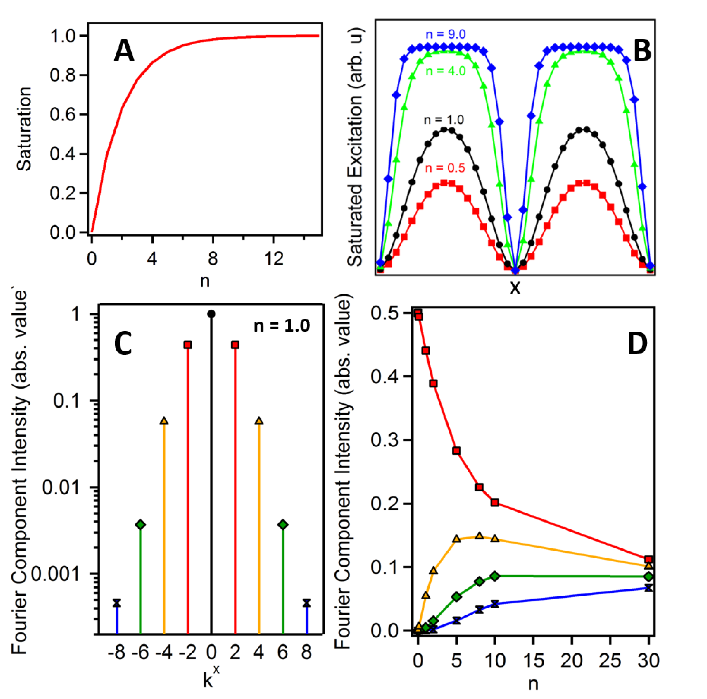
Figure 2.
Comparison of LF-SSEM optical transfer functions (OTFs) with utilization of higher order Fourier components. The black trace shows the diffraction-limited (DL) OTF. The red traces show the initial OTF (dashed) produced by image reconstruction and the final OTF (squares) trace after amplitude normalization when including only first-order (linear) Fourier components. Blue (triangles), green (diamonds) and yellow (hourglasses) traces represent the normalized OTFs when incorporating the k = ±4kx, ±6kx and ±8kx components, respectively. Note that the higher order OTFs are renormalized to an amplitude larger than 1.0 for visibility.

Figure 3.
(A) Profile comparison of the DL and LF-SSEM model point spread functions (PSFs). The black dashed trace is the DL model with the full width at half maximum (FWHM) normalized to 1. The red (squares) and green (circles) traces show LF-SSEM PSFs including Fourier components up to k = ±2kx and k = ±8kx, respectively. (B) Reduction of the optical PSF FWHM with the inclusion of higher order Fourier components.
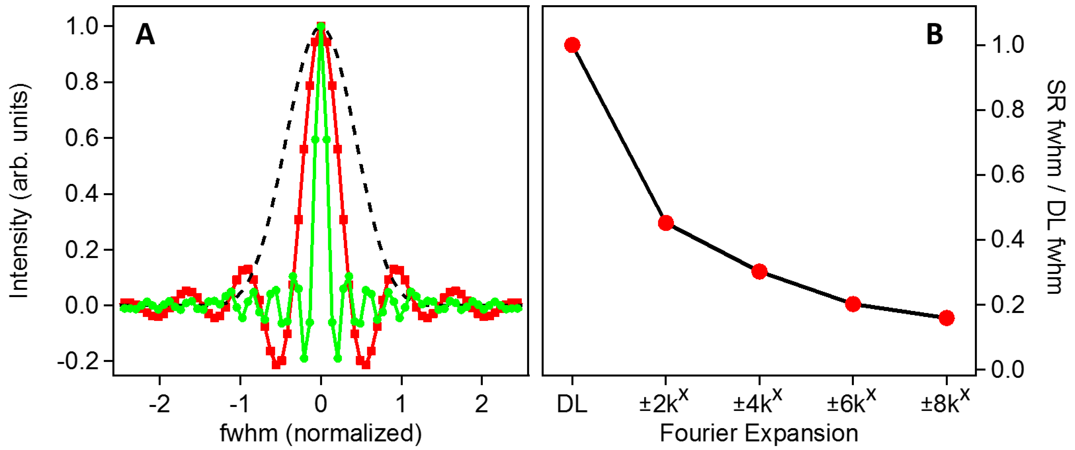
Figure 4.
Imaging a one-dimensional grating using both DL and LF-SSEM models. (A) Simulated target image with individual component dimensions ranging from 30 nm to 180 nm. (B–D) Images produced by using the DL model (B) and the LF-SSEM model (C, D). Panels C and D show images determined using the LF-SSEM model with Fourier expansions of ±2kx and ±8kx, respectively. (E–H) Profile comparisons of the three separate images in Panels B (red), C (green), and D (blue). The length scale below Panel D applies to all images in the left column and corresponds to the individual truncated length scales in the right column. The color scale in Panel A corresponds to Panels A–D.

Figure 5.
Signal-to-noise ratio (SNR)-dependent LF-SSEM image reconstruction using 784 nm excitation and 900 nm probe wavelengths. Panel A shows the profiles of three structured image spectra with varying SNRs given in the legend. Panel B shows the resulting PSF of the optical system after image reconstruction using Fourier components that exceeded the SNR. The DL model shows a FWHM of 432 nm. The green (triangles), blue (squares) and red (circles) show the PSF resulting from the use of ±2kx, ±4kx and ±6kx Fourier expansions, respectively.

© 2017 by the authors. Licensee MDPI, Basel, Switzerland. This article is an open access article distributed under the terms and conditions of the Creative Commons Attribution (CC BY) license (http://creativecommons.org/licenses/by/4.0/).
Share and Cite
MDPI and ACS Style
Massaro, E.S.; Grumstrup, E.M. Label-Free Saturated Structured Excitation Microscopy. Photonics 2017, 4, 36. https://doi.org/10.3390/photonics4020036
AMA Style
Massaro ES, Grumstrup EM. Label-Free Saturated Structured Excitation Microscopy. Photonics. 2017; 4(2):36. https://doi.org/10.3390/photonics4020036
Chicago/Turabian StyleMassaro, Eric S., and Erik M. Grumstrup. 2017. "Label-Free Saturated Structured Excitation Microscopy" Photonics 4, no. 2: 36. https://doi.org/10.3390/photonics4020036
Note that from the first issue of 2016, this journal uses article numbers instead of page numbers. See further details here.