Exploring the Potential of Airyscan Microscopy for Live Cell Imaging


1
Kennedy Institute for Rheumatology, Roosevelt Drive, University of Oxford, Oxford OX3 7LF, UK
2
Wolfson Imaging Centre, Weatherall Institute of Molecular Medicine, University of Oxford, Headley Way, Oxford OX3 9DS, UK
3
MRC Human Immunology Unit, Weatherall Institute of Molecular Medicine, University of Oxford, Headley Way, Oxford OX3 9DS, UK
*
Author to whom correspondence should be addressed.
Photonics 2017, 4(3), 41; https://doi.org/10.3390/photonics4030041
Submission received: 1 June 2017
/
Revised: 19 June 2017
/
Accepted: 30 June 2017
/
Published: 7 July 2017
(This article belongs to the Special Issue Superresolution Optical Microscopy)
Abstract
:Biological research increasingly demands the use of non-invasive and ultra-sensitive imaging techniques. The Airyscan technology was recently developed to bridge the gap between conventional confocal and super-resolution microscopy. This technique combines confocal imaging with a 0.2 Airy Unit pinhole, deconvolution and the pixel-reassignment principle in order to enhance both the spatial resolution and signal-to-noise-ratio without increasing the excitation power and acquisition time. Here, we present a detailed study evaluating the performance of Airyscan as compared to confocal microscopy by imaging a variety of reference samples and biological specimens with different acquisition and processing parameters. We found that the processed Airyscan images at default deconvolution settings have a spatial resolution similar to that of conventional confocal imaging with a pinhole setting of 0.2 Airy Units, but with a significantly improved signal-to-noise-ratio. Further gains in the spatial resolution could be achieved by the use of enhanced deconvolution filter settings, but at a steady loss in the signal-to-noise ratio, which at more extreme settings resulted in significant data loss and image distortion.
1. Introduction
Optical microscopy has increasingly become an important tool for biomedical research. In recent decades, fluorescence-based imaging technology has made a great leap forward from basic wide-field microscopes to complex super-resolution imaging systems [1,2,3,4]. To-date, modern fluorescence microscopy offers diverse opportunities to specifically label and study the dynamics of single or multiple molecules, protein clusters and/or complete structures of interest at unprecedented detail [5,6,7]. Consequently, a myriad of imaging modes is available as turn-key commercial setups [5]. However, maintaining a good balance between spatial and temporal resolution without sacrificing the photon budget, as is evident by the fluorescence signal intensity and image contrast, remains a challenging task [5,8,9,10]. These parameters are especially important for live cell imaging, where it is often crucial to be able to distinguish sub-cellular features, while also being able to track dynamical processes at low illumination densities in order to minimise the phototoxic damage of the biological specimen. On the one hand, wide-field approaches are optimal in terms of readout speed and photo-toxicity, but have compromised spatial resolution, at the diffraction limit, which limits its use for subcellular morphological studies [8]. In contrast, super-resolution approaches provide access down to a few tens of nanometres scale, but at the expense of high power density and long acquisition speeds, making them not preferential for live cell imaging [9]. Stochastic-Optical-Reconstruction-Microscopy (STORM) and Photo-Activated-Localization-Microscopy (PALM) allow, for instance, the accurate localization of proteins within dense interwoven protein clusters and cytoskeletal networks [4,11,12,13,14], but their use is restricted almost exclusively to fixed samples. In contrast, three-Dimensional (3D) Stimulated-Emission-Depletion (STED) microscopy offers a good compromise between increased spatial (~40–100 nm laterally and 300 nm axially) and temporal resolution, but in this case, at the expense of small fields of view and shorter periods of time compared to confocal microscopy [9,15,16,17]. Advanced wide-field-based methodologies, such as TIRF (Total-Internal-Reflection-Fluorescence) and 3D Structured-Illumination-Microscopy (SIM), have demonstrated a great ability to monitor the dynamics of cytoskeletal structures over time and at extended spatial resolution compared to confocal [9,18]. Yet, the spatial resolution of SIM (~120 nm laterally and 300 nm axially) is limited compared to STED and STORM/PALM. Additionally, such state-of-the-art super-resolution microscopes are generally more costly, dedicated for advanced users and require more rigorous sample preparations [8]. For that reason, the confocal-based fluorescence still remains one of the most accessible optical microscopes, because in spite of its relative simplicity, it can provide sufficient readout speed together with good optical sectioning at comparably low cost [19].
Confocal microscopy produces a fluorescent image as a convolution of the specimen of interest and it’s Point-Spread-Function (PSF). In a conventional confocal system the PSF depends on the excitation wavelength, numerical aperture of the objective and the pinhole diameter, such that the usage of high numerical aperture (NA) objectives and minimal pinhole diameter can significantly improve the image quality including the spatial resolution and Signal-to-Noise Ratio (SNR). Specifically, confocal microscopy by its design is able to offer up to factor of √2 spatial resolution improvement compared to wide-field approaches, by rejecting out of focus light at the confocal pinhole [20]. Unfortunately, maximal spatial resolution enhancement can only be achieved with the use of an infinitely small pinhole, which is practically not possible as none of the emitted photons would reach the detector. Consequently, the opening of the pinhole is usually set to one Airy Unit (AU), a setting at which the pinhole size matches the diameter of the central Airy disk of the diffraction pattern and thus provides the best-possible compromise between spatial resolution and SNR [20]. For bright fluorescent samples, the pinhole size can be further reduced from 1 AU down to 0.5 AU or even 0.2 AU, in order to yield an additional improvement in the spatial resolution and contrast of the fluorescent image.
Substantial efforts have been devoted to finding ways to further improve the performance of confocal microscopy without a dramatic increase of neither the cost, nor the complexity of the system. Improving the spatial resolution in this context means obtaining more structural information about a specimen or, in simple terms, more data containing higher spatial frequency components of an image. This can be achieved at a hardware or software level, or via the combination of both components [21]. Among common approaches for recovering high spatial frequencies are deconvolution [22], re-scan [23], subtraction [24,25] and pixel-re-assignment [26] of images. The most commonly used among those techniques are the image deconvolution methods that employ prior knowledge of the system’s PSF for spatial resolution enhancement. The PSF of the microscope can be either theoretically computed or, for the best result, measured for each dataset [22]. A common practice in this case is the application of the Wiener filter approach to minimise the impact of frequencies with low SNRs on the reconstructed images [27]. Combining this knowledge with the fitting complexity of deconvolution algorithms can make this method challenging to assess and employ for an unprepared user. Alternatively, subtraction and re-scan methods require that at least two images are acquired for the subsequent image processing. This doubles the acquisition times and hence is not preferential for live cell studies as longer exposure times increase the loss of fluorescence due to photo-bleaching and photo-damage [5,25]. In this regard, hardware improvements allowing a combination of these techniques appear more advantageous. Of particular interest is a novel method whereby the physical confocal pinhole is replaced with an adapted detector array or CCD (Charge-Coupled-Device) camera, allowing the collection of more light and thus additional structural data. This approach is realised in pixel reassignment and Airyscan methods [28,29].
The Airyscan technology is designed to improve the spatial resolution and SNR by exploiting a combination of the equivalent of confocal imaging with a 0.2-AU pinhole setting, Wiener filter-based deconvolution and the pixel reassignment principle [26]. Airyscan was recently introduced as an extension of the pixel-re-assignment technique developed by Sheppard et al. [26] and the pinhole-plane imaging systems independently proposed by Bertero [30] and Sheppard [31]. All of these approaches benefit from the collection of all of the emitted light, which otherwise would be rejected at the pinhole in a conventional confocal architecture. When a camera or detector array is placed within the conjugated plane instead of a confocal aperture, each of the detection elements are acting as a separate pinhole. By knowing the dimension of each element, together with its displacement from the optical axis, the improved image can be reconstructed [29]. To further extend this, more detectors can be used in the system; thus, more datasets are collected, and consequently, a more prominent improvement can be expected. The Zeiss Airyscan (see the Section 2) compound detector consists of 32 elements, each of them equivalent to a point detector sampled with a 0.2-AU pinhole. These 32 elements are arranged in a circular geometry, such that the total detector area is equivalent to a 1.25-AU pinhole setting (Figure 1). As a result, the spatial resolution of the final reconstructed image is defined by the sampling of the central pixel, which in this case is comparable to images acquired with conventional confocal at 0.2 AU, while the total sensitivity of the system is expected to be equivalent to a confocal image acquired at 1.25 AU [29,32]. Further resolution gains can be achieved by the use of a Wiener filter-based deconvolution step during image reconstruction. This hardware configuration allows simultaneous acquisition using all 32 channels, at acquisition rates comparable to conventional detection setups of ordinary confocal, albeit the Airyscan approach is currently limited to sequential multi-colour imaging.
All aforementioned properties are thought to make Airyscan microscopy a good candidate for improved dynamic live cell imaging, because it has all of the advantage of confocal microscope together with enhanced spatial resolution and increased fluorescence signal sensitivity [33]. However, to our knowledge, no rigorous study of Airyscan microscopy has been performed to test its potential for biological studies.
Here, we present a systematic comparative study of the performance of the Airyscan modality compared with conventional confocal. We focused on analysing the degree of spatial resolution enhancement and SNR for standard reference samples, as well as for biological specimens. We compared various reference sample images in both confocal and Airyscan modalities in order to try to understand how the sample brightness and morphology influence the performance of the Airyscan processing algorithm. We found that processed Airyscan images, at the automatic default Wiener filter settings, have a spatial resolution equivalent to that of 0.2 AU, but with significantly improved SNR, making Airyscan a promising candidate for live cell dynamical studies.
2. Materials and Methods
2.1. Cell and Tissue Culture
2.1.1. HeLa Cells
Cervical HeLa cells (Product 93021013, Sigma Aldrich, Irvine, UK; mycoplasma tested) were cultured in sterile RPMI media (Sigma Aldrich, Irvine, UK) supplemented with 10% FCS (Sigma Aldrich, Irvine, UK) and 1% penicillin-streptomycin-neomycin solution (Sigma Aldrich, Irvine, UK). Cells were maintained at 37 °C and 5% CO2 during cell culture.
2.1.2. Immunostaining of Nuclear Pore Samples
HeLa cells were passaged to grow on high performance glass coverslips (thickness = 0.17 mm; Carl Zeiss, Oberkochen, Germany, Prod # 474030-9010-000) for at least 48 h. Cells were subsequently washed in Phosphate-Buffered Saline (PBS; Life Technologies, Carlsbad, CA, USA, Prod # 10010-015) and fixed in 4% methanol-free formaldehyde (Thermo Scientific, Waltham, MA, USA, Prod # 11586711) in PBS at Room Temperature (RT) for 10 min. Cells were then washed 3 times in PBS, permeabilized for 5 min at RT in 0.1% Triton X-100 (Sigma-Aldrich; Prod # 93443) in PBS, washed 3 times in PBS and blocked to minimise non-specific binding in MAXblock™ Blocking Medium (Active Motif, Carlsbad, CA, USA, Prod # 15252) for 1 h at RT.
HeLa cells stained for the Nuclear Pore Complexes (NPC) were stained with 1 μg/mL of a mouse monoclonal to Nup153 (Clone QE5; Abcam Plc, Cambridge, UK, Prod # ab24700) diluted in PBS with 1% BSA (Sigma-Aldrich; Prod # A7906) overnight at 4 °C. Cells were then washed 3 times in PBS and stained with a 1:500 dilution of Abberior Star Red labelled goat anti-mouse IgG (Abberior GmbH, Göttingen, Germany, Prod # 2-0012-011-2) for 2 h at RT. Cells were again washed 3 times in PBS, mounted with Slowfade Diamond Antifade Mountant (Thermo Fisher, Waltham, MA, USA, Prod # S36963), a glycerol based non-hardening mounting media, and sealed with nail polish.
2.1.3. Rat Basophilic Leukaemia Cells
Rat Basophilic Leukaemia (RBL)-2H3 clone cells (CRL-2256, ATCC, Manassas, VA, USA) were cultured at 37 °C in 5% CO2 in Minimum Essential Media (MEM) (Sigma Aldrich) supplemented with 10% FBS, 10 mM HEPES (Lonza, Slough, UK), 1% penicillin streptomycin and 1% L-glutamine. Cells were split every two days at a volume ratio of 1:5. Twenty four hours prior to experiments, adherent cells were treated with 0.05% Trypsin-EDTA (Lonza), facilitating their detachment from the cell culture flask. Cells were then transferred to a rotating chamber at 37 °C in 5% CO2 to maintain their suspensions state prior to the experiments.
2.1.4. Plasmids
To obtain vectors C-terminally-tagged encoding LifeAct-citrine (New England Biolabs, Ipswich, UK) and FCεR-snap, the genes were amplified by PCR to produce dsDNA fragments encoding LifeAct and FCεR sequences followed by a Gly-Ser linker and flanked by 5′ MluI and 3′ BamHI restriction nuclease sites. Following digestion with MluI and BamHI, this was ligated into pHR-SIN lentiviral expression vectors containing the mCitrine and snap gene downstream of the BamHI site in the correct reading frame. Sequence integrity was confirmed by reversible terminator base sequencing. Detailed information is presented in [18].
2.1.5. Generation of Stable RBL Cell Lines
RBL cell lines stably expressing LifeAct-citrine and FCεRI-snap were generated using a lentiviral transduction strategy. HEK-293T cells were plated in 6-well plates at 3 × 10⁵ cells/mL, 2 mL/well in DMEM + 10% FBS. Cells were incubated at 37 °C and 5% CO2 for 24 h before transfection with 0.5 μg/well each of the lentiviral packaging vectors p8.91 and pMD.G and the relevant pHR-SIN lentiviral expression vector using GeneJuice (Merck Millipore) as per the manufacturer’s instructions. At 48 h post transfection, the cell supernatant was harvested and filtered using a 45-μm Millex-GP syringe filter unit to remove detached HEK-293T cells. Three millilitres of this virus-containing medium were added to 1.5 × 10⁶ RBL cells in 3 mL supplemented RPMI-1640 medium. After 48 h, cells were moved into 10 mL supplemented MEM and passaged as normal.
2.2. Experimental Setup
Airyscan imaging was performed with a confocal laser scanning microscope ZEISS LSM 880 (Carl Zeiss AG, Oberkochen, Germany) equipped with an Airyscan detection unit. To maximize the resolution enhancement, we used high NA oil immersion alpha Plan-Apochromat 63X/1.46 Oil Corr M27 or Plan-Apochromat 63X/1.40 Oil Corr M27 objectives (Zeiss). All imaging was performed using Immersol 518 F immersion media (ne = 1.518 (23 °C); Carl Zeiss). Detector gain and pixel dwell times were adjusted for each dataset keeping them at their lowest values in order to avoid saturation and bleaching effects. Laser intensity values at the sample plane were measured with a Microscope Slide Thermal Sensor (Thorlabs, Newton, NJ, USA).
2.2.1. GATTA-Beads
GATTA-Beads (Gattaquant, Braunschweig, Germany) are DNA-based fluorescent calibration beads with a diameter of 23 nm. In this work, we used the beads of red (ATTO 647 N) and blue (Oregon Green 488) colours (http://www.gattaquant.com/products/gatta-beads.html). The beads were fixed on the cover glass slide.
Microscopy images of GATTA-Beads were acquired as z-stacks on a Zeiss 880 inverted confocal with a 63X 1.40 NA oil immersion objective. The acquisition was performed for 11 z-planes with a pixel size of 41 nm × 41 nm and a z-spacing of 150 nm centred at the plane of sharpest focus. Images were saved in .czi format. Conventional confocal images were acquired with 5% of maximum laser power, corresponding to ≈10 μW at the focal plane for both the 488-nm and 633-nm laser lines, with a main beam splitter MBS488/561/633 and with emission filter settings with about a 50-nm bandwidth from near the respective excitation lines. Images were acquired with pinhole settings of either 0.2 or 1 AU, on a GaAsP-PMT detector with a gain setting of 800, a pixel dwell time of 2.06 μs and no averaging. Airyscan images were acquired with 2% of maximum laser power, corresponding to ≈4 μW for both the 488 nm and 633 nm laser lines and with a main beam splitter MBS488/561/633, no additional emission filter, a gain setting of 750, a pixel dwell time of 2.06 μs and no averaging.
2.2.2. TetraSpeck Beads
The TetraSpeck™ Fluorescent Microsphere Standard slide (Invitrogen, Carlsbad, CA, USA) was used as the 200-nm bead sample. The microspheres with 200 nm in diameter are stained throughout with four different fluorescent dyes of the following colours: 365/430 nm (blue), 505/515 nm (green), 560/580 nm (orange) and 660/680 nm (dark red). The beads are mounted on the cover slide with a density of ~2.3 × 10¹⁰ particles/mL.
Images were acquired on a Zeiss 880 inverted confocal with a 63X 1.46 NA oil immersion objective, with the following parameters: excitation wavelength 488 nm, a pixel size of 41 nm × 41 nm, emission filter BP496-550 and no averaging. The imaging plane was selected as having the sharpest focus. Images were saved in .czi format.
2.2.3. Argolight SIM Slide
All images of the Argo-SIM slide (Argolight, Pessac, France) were acquired as z-stacks on a Zeiss 880 inverted confocal with a 63X 1.40 NA oil immersion objective. For evaluation of the lateral resolution in the blue part of the visible spectra, we used 405-nm laser excitation, a pixel size of 34 nm × 34 nm, a z-spacing of 140 nm and by acquisition of 11 z-planes, centred at the plane of sharpest focus. Images were saved in .czi format.
Conventional confocal images were acquired with 5% of maximum 405 nm laser power (≈10 μW), a pinhole setting of 1 Airy Unit (AU; pinhole diameter of 42 μm) and with a bandpass emission of 410–481 nm, on a conventional PMT detector with a gain setting of 650, a pixel dwell time of 1.71 μs and no averaging. Airyscan images were acquired with 2% of the maximum 405-nm laser power (≈4 μW) with a main beam splitter MBS405, no additional emission filter, a gain setting of 700, a pixel dwell time of 1.09 μs and no averaging. Airyscan processing was done in 3D mode either at default settings or with a manual setting of the filter strength as noted.
2.2.4. Nuclear Pore Complexes in HeLa Cells
NPC imaging was performed using an Apochromat 63X/1.40 Oil immersion objective with 633-nm laser excitation with typical laser powers in the focal plane of 5–10 μW. Image stacks were acquired with a pixel size of 41 nm × 41 nm and a z-spacing of 150 nm, a detector gain setting of 700 and a pixel dwell time of 1.09 μs.
2.2.5. Microscopy Cover Slide Preparation
IgE-coated coverslips were prepared by coating high-NA cover-slips (Zeiss, Germany) with BSA-TNP at a concentration of 500 μg/mL and incubating at 4 °C overnight. Coverslips were washed 3 times using PBS, followed by the addition of a 10% solution of BSA for a further hour at room temperature. Following this, coverslips were washed 3 times in PBS and then coated with a 5-µg/mL IgE for 1 h at room temperature. Following incubation, coverslips were washed a further 3 times in PBS before being used at the microscope.
2.2.6. Rat Basophilic Leukaemia Live-Cell Imaging
All RBL live-cell experiments were done at 37 °C and 5% CO2. A diode laser at 561 nm and argon laser light at 488 nm were used as fluorescence excitation sources. Excitation powers were set at 1–3% for both lasers (1–5 μW) and were adjusted within this range for each image individually in order to achieve a strong enough fluorescence signal for both channels. Fluorescence emission was collected at around 595 nm and 515 nm for the red and green channels, respectively, with the filters BP570-620 + LP645 (red) and BP420-480 + BP495-550 (green). The image time series were acquired with 10-second time interval between the measurements to minimise photo-bleaching and photo-toxicity. The emission signals for both channels were collected subsequently on the 32-channel GaAsP-PMT Airy detector. Airyscan time series measurements were performed in at least 10 individual cells for each experimental condition over the course of 5 independent experiments.
2.2.7. SNAP-Tag Labelling
RBL cells expressing the SNAP-tag (New England Biolabs) fusion protein were labelled with SNAP-Cell TMR-Star following the manufacturer’s preparation protocol (www.neb.com). The cell medium was first replaced with 200 μL of SNAP-tag medium Leibovitz’s L-15 medium (Life Technologies) with 1–5 μM SNAP-tag ligand and then incubated for 45 min at 37 °C in an Eppendorf thermo-mixer (Eppendorf Ltd, Stevenage, UK) at 300 rotations per min (rpm). Finally, to ensure that free dye would not remain in the cytoplasm, the cell-labelling solution was washed three times in L-15 and then further incubated for 30 min at 37 °C in a thermo-mixer at 300 rpm.
2.3. Airyscan Processing
Zen Black 2.1 (Version 13.0.0.0) software was used to process the acquired datasets. The software processes each of the 32 Airy detector channels separately by performing filtering, deconvolution and pixel reassignment in order to obtain images with enhanced spatial resolution and improved SNR. This processing includes a Wiener filter deconvolution with options of either 2D or a 3D reconstruction algorithm (details are described elsewhere [32]). For simplicity, we henceforth refer to this post-processing algorithm as Airyscan Filtering (AF). There are furthermore options for the user to choose either the automatically-determined default AF filter strength or manual filter strength with a range of values from 1 to 12. Those values refer to the Wiener parameter 10(−f) where f is the Airyscan filter strength. Finally, there is an option for applying an intensity bias consisting of an Airyscan Processing Baseline Shift of 10,000 intensity units; otherwise, negative intensity values in a reconstructed image are cropped to zero. In our analysis, we applied the Airyscan Processing Baseline Shift and further used the 2D or 3D reconstruction algorithm either at the default filter setting or at filter settings as noted.
2.4. Data Analysis
2.4.1. Determination of the Spatial Resolution
In optical microscopy, several criteria exist to define the spatial resolution of a given imaging system, which describes the ability of a microscope to discriminate constituent parts of an object with a certain level of distinction [21]. We employ the two most commonly-used definitions: the Full Width at Half Maximum (FWHM) criterion of a given PSF and the Rayleigh criterion. We used the FWHM criterion to determine the spatial resolution of fluorescent beads and NPC reference samples because the criterion is optimised to measure the spatial resolution of individual fluorescently-tagged point source objects. Complementary to this, the Rayleigh criterion describes the ability of a microscope to resolve two point sources, of equal intensity, as two separate objects. Consequently, the Rayleigh criterion is especially useful to determine the spatial resolution of the Argo-SIM reference sample (see Section 2.4.3) because it is optimised to compare the resolvable distance of fluorescent objects. Detailed information about the FWHM and Rayleigh criterion is reviewed in [21].
2.4.2. Fitting of Fluorescent Bead Reference Samples and NPC Samples
The resolution of 2D bead and NPC images was determined using a custom-written MATLAB routine. For each image, the locations of the fluorescent beads were established using a feature detection algorithm (people.umass.edu/kilfoil/downloads). After filtering non-circular objects, each feature pixel intensity distribution was fitted with a 2D Gaussian function and the FWHM extracted for on the order of 200–300 beads per condition. The FWHMs of the beads within a given image displayed a Gaussian distribution, and hence, the mean FWHM and standard deviation were recorded for each image.
2.4.3. Argo-SIM Slide Reference Samples
Image analysis was performed by a combination of the Fiji version of ImageJ (v 1.51 g) and Mathematica v11 (Wolfram, Long Hanborough, UK). In the analysis, we first imported the czi images in Fiji by use of the Bioformat plugin. We subsequently identified the central focal plane and proceeded by measuring the line intensity profile, with a line width of ten pixels, perpendicular to the direction of the lines on the Argo-SIM slide test pattern at n = 6 positions per condition. The intensity values of the line profiles were saved in text format and imported in Mathematica for further quantitative regression analysis of the intensity profiles corresponding to the central pair of lines for each specified line spacing from 90 to 390 nm in steps of 30 nm to the sum of two 1D spatial Gaussian functions.
The free parameters of this fit were the intensity of the background fluorescence, Ibkgd, the peak intensities of each separate line, Ipeak1 and Ipeak2, the central positions of each separate line, xpeak1 and xpeak2, and the Gaussian width of each separate line, σpeak 1 and σpeak 2.
From the resulting fit parameters, we determined the distance of separation between the two intensity peaks from:
and the Full Width Half Maximum (FWHM) of each intensity peak as:
A linear regression of the fitted results for the separation between the two intensity peaks as described versus the specified line separation resulted in a y-intercept of 97 ± 4 nm and a slope of 1.0 ± 0.0, suggesting that the line width of the Argo-SIM test pattern in the blue emission channel was about 100 nm.
We further evaluated the relative dip in the intensity between the two central lines by calculating:
where Ipeak1 and Ipeak2 were the fitted peak intensities and Imin was the minimum intensity of the fit in between the fitted positions of each separate line, xpeak1 and xpeak2. A trend line for this data was generated by fitting the results to an interpolating polynomial
2.5. Determination of the SNR
We analysed the SNR of raw and processed images of the Argo-SIM resolution pattern by quantifying the intensity fluctuations relative to the mean intensity of the line features. For this, we selected line profiles with a line width of 1 pixel and a length of 850 pixels, parallel to the direction of the line features and super-imposed on the lines of the Argo-SIM slide test pattern. The mean signal, Sn, (± the standard deviation) for each image condition was determined by calculating the mean intensity Sn for each line profile:
where In(y) is the intensity of line profile n at pixel y. We next calculated the mean signal, S, and the standard deviation of the mean signal, ΔS, for each image condition using standard methods with n = 6 positions per condition.
We computed the mean noise Nn as the standard deviation of the difference between the mean signal, S, and the raw intensity data, In(y), for each line profile, n, at each pixel, y:
and the mean noise, N, and standard deviation of the mean noise, ΔN, using standard methods with n = 6 positions per condition.
The SNR was then computed as the ratio of the mean signal and the mean noise (± the standard deviation) by use of standard error propagation.
3. Results
3.1. Evaluation of the Spatial Resolution and Signal-To-Noise Ratio Using Bead Reference Samples
In this study, we used the commercial Zeiss 880 inverted confocal system with a 32-element Airyscan detector (see the Section 2; Figure 1a,b). To evaluate the performance of the Airyscan technique, we imaged two different-sized bead reference samples: 23-nm GATTA-Beads and 200-nm TetraSpeck beads (see the Section 2).
In these experiments, the FWHM of the PSF was used to reflect the resolving power of an optical system. The PSF can be measured experimentally by imaging fluorescent beads or other point source objects with dimensions much smaller than the diffraction limit. We used 23-nm fluorescent beads (GATTA-beads labelled with either of the dyes Oregon Green 488 or Atto647N), deposited on the cover slide and imaged at 488-nm and 633-nm excitation wavelengths, respectively. The blue and red excitations were chosen to account for possible chromatic effects at both ends of the visible spectra. Figure 2a compares the PSFs of 23-nm diameter Oregon Green 488-labelled beads in the axial (Z) and lateral (XY) direction between conventional confocal with a pinhole diameter of 0.2 AU and the Airyscan post-processed images at different manually-selected Airyscan filter strengths of AF4 (AF4 refers to AF = 4), AF6 and AF8, respectively. Visual inspection of the representative fluorescent images of the 23-nm beads clearly indicated that the FWHM was dependent on the AF strength such that the FWHM decreases with increasing AFs (Figure 2b). To this end, the spatial resolution of the bead images was significantly smaller at low AFs (AF4) compared to images acquired at 0.2-AU pinhole diameters in confocal. At high AFs, the images comprised obvious image distortion and high spatial frequency noise artefacts (AF8; Figure 2a).
To quantify these changes, we fit the individual PSFs of the 23-nm GATTA-beads and 200-nm TetraSpeck beads for both excitation wavelengths, using custom-written MATLAB algorithms (see Section 2). Note in the following, for reasons of simplicity that we only report changes of the PSFs in the lateral direction, but all findings apply also for the axial direction of the PSFs, except where otherwise indicated. We first sought to quantitatively verify the improvement in the spatial resolution of the Airyscan approach relative to conventional confocal imaging with a standard pinhole setting of 1 AU and with a more restricted pinhole setting of 0.2 AU (Figure 2b). We found that the spatial resolution, as determined from the FWHM of 23-nm diameter GATTA-Beads labelled with Atto647N and imaged at 633-nm excitation, was as expected enhanced by about ≈1.2X even in conventional confocal imaging when closing the pinhole from a standard setting of 1 AU–0.2 AU. We further found that the spatial resolution of the reconstructed Airy sum of the raw Airyscan data, which corresponds to a pinhole setting of 1.25 AU, as well as the raw data from Channel 1 of the Airyscan detector, which corresponds to a pinhole setting of about 0.2 AU, were in close agreement with the equivalent conventional confocal settings (Figure 2b).
Image reconstruction of the raw Airyscan data involves a Wiener filter protocol. While the Zen software offers an automatic setting for determining the filter strength, we sought to directly quantify the effect of the Wiener filter strength on the spatial resolution of the processed images (Figure 2b). We re-constructed raw Airyscan data of the same 23-nm diameter GATTA-Beads labelled with the far red dye Atto647N at various filter settings. This analysis revealed that there was a direct, approximately linear, dependence between the filter strength and the resulting spatial resolution. The spatial resolution of the sample at the default filter setting was about ≈220 ± 20 nm. This was comparable with conventional confocal data with a pinhole setting of 0.2 AU or to the raw Airyscan data from Channel 1 only, but a 1.3 times improvement as compared to conventional confocal imaging at 1 AU.
We further investigated the effects of signal intensity and raw signal noise level on the determination of the default Wiener filter in the image re-construction and by extension on the spatial resolution of the image (Figure 2b). For this, we imaged the GATTA-Beads at different laser excitation power (to probe the effect of the signal dependence) and at different line averaging settings (to probe the effect of the noise). These results demonstrated a weak dependence on the strength of the default filter setting when using line averaging. These results further showed that the default filter setting is minimally increased for higher excitation laser powers and did not result in a corresponding improvement in the spatial resolution.
We also examined the relationship between the excitation wavelength and the AF filter settings by comparing GATTA-Beads labelled with Orgeon Green 488, excited with a 488-nm laser line, or Atto647N, excited with a 633-nm laser line. For both excitation wavelengths, we found that increasing AFs significantly reduced the FWHMs of the bead reference samples (black filled circles show 633-nm excitation and purple filled triangles 488-nm excitation wavelengths). Specifically for the 23 nm, the FWHMs were reduced from 277 ± 35 nm at AF4 to 121 ± 31 nm at AF8; compared to conventional confocal at 293 ± 28 nm at 1 AU and 244 ± 28 nm at 0.2 AU; suggesting that increasing AF indeed improves the spatial resolution, and the AF8 settings yield up to two-fold resolution improvement compared with 0.2-AU confocal.
To understand whether high AF levels may over-improve the spatial resolution (to the values below the original size of a feature), we imaged 200-nm TetraSpeck beads. In addition, to ensure that the brightness of the sample did not affect the final spatial resolution, the imaging was carried out at several illumination levels between 2 and 8% laser power. Trends were similar for all of the excitation powers, and only broadening effects of the FWHM were observed (Figure 2c, non-solid symbols). Notably, the FWHM for 200-nm beads at low AF settings remains constant and comparable to the confocal 1 AU value (254 ± 17 nm and 251 ± 25 nm). The reduction of FWHM occurred only at values of AF greater than six. The increase of the filtering strength to AF8 allows achieving resolution comparable to confocal with a pinhole diameter of 0.2 AU, but at higher values (AF9), the FWHM is further reduced to 169 ± 14 nm, which is far smaller than the actual physical size of the beads.
Next, we investigated whether the brightness of the reference sample affected the final spatial resolution post-AF processing. For that, the detector gain was kept constant for all power settings ranging from 2 to 8% laser power, avoiding signal saturation at maximal power. Figure 2c shows how the overall trend of the changes in the FWHM as a function of the AF settings was similar for all of the excitation powers, but spatial broadening of the FWHM was observed at higher values. Specifically, the results suggested that the improvements in spatial resolution of the GATTA-Beads and TetraSpeck beads were constant for low AFs and comparable to the confocal 1 AU value (254 ± 17 nm and 251 ± 25 nm, respectively). Further, AFs greater than the value of six yielded smaller FWHMs. For AF8, the spatial resolution achieved values comparable to 0.2 AU confocal. The FWHM of the 200-nm TetraSpeck beads could be further reduced to 169 ± 14 nm at AF9, suggesting that Airyscan post-processing can result in artefactual object size consistently for several laser powers.
3.2. Determination of the Spatial Resolution and Signal-To-Noise Ratio Using Argolight-SIM Slide
Having determined the spatial resolution and SNR for conventional bead reference samples by the FWHM criterion, we next evaluated these parameters using the Rayleigh criterion (see the Section 2). For this, we utilised an Argolight-SIM test slide (referred to later as Argo-SIM), which consisted of pairs of lines with gradually increasing central line spacing, from 0 to 390 nm, with a step size of 30 nm (Figure 3). Complementary to the bead reference sample, the Argo-SIM slide offered a systematic protocol to evaluate the ability of the Airyscan microscope to resolve nearby objects, such as two lines as a function of the line spacing. To this end, it allowed both a qualitative evaluation by direct inspection of the images and quantitative image analysis followed by a direct comparison to the resolution limit specified by the Rayleigh criterion, which in the case of a circular aperture corresponds to a saddle intensity point between the respective peak intensities of the two point sources, of equal peak intensity Ipeak, where the relative intensity is given by:
where J1 is the Bessel function of the first kind of order one and j1,1 is the first zero of the Bessel function of the first kind of order one and which is equal to ≈3.8317.
Consistent with the bead reference samples, we found that the spatial resolution improved with increasing AFs (Figure 3a–j). In particular, the Airyscan imaging was able to resolve the central pairs of lines in the case of conventional confocal imaging with the pinhole diameter 1 AU down to a spatial resolution of 180–210 nm, as expected for a confocal microscope in the blue part of the visible spectra. Further post-processing at default AF (AF5.9) yielded an improved resolution in the region of 150 nm (Figure 3f) and with additional resolution gains down to a FWHM of around 120 nm at AF9. Similarly to the bead samples, high AFs resulted in high frequency noise, including the appearance of negative intensities, which is evident both directly by the distinct intensity fluctuations in the close-up images and from the highlighted intensity Regions Of Interest (ROIs; blue rectangles) in the exemplary line intensity profiles (Figure 3f–j). Inspection of the exemplary line intensity profiles also suggested that the default filter setting in the Airyscan processing was set to prevent the appearance of high-frequency noise in the re-constructed image as evidenced by the absence of negative intensities in the highlighted intensity ROIs (blue rectangles) in Figure 3f, as opposed to the increased presence of negative intensities in Figure 3g–j. This artefact of high frequency noise in the re-constructed images was similar to image reconstruction issues associated with SIM data [34].
To further illustrate these findings of the Argo-SIM slide, we performed a systematic quantitative analysis of the spatial resolution and the SNRs. To determine the distance between two subsequent lines and thus the spatial resolution measured at the Argo-SIM slide, we employed non-linear regression fitting. To this end, our algorithm was set to detect the mean drop in the intensity between the central pairs of lines as a function of the specified line separation (Figure 4a), where the required relative intensity drop should satisfy ΔI/Ipeak ≳ 0.265 (Rayleigh criterion; see the Section 2). Figure 4a confirmed the previous qualitative inspection shown in Figure 3 that the lateral spatial resolution was 200 nm for the case of confocal imaging with a pinhole setting of 1 AU. In contrast, the Airyscan data from Channel 1 (equivalent of 0.2 AU) yielded an improved spatial resolution of about 150 nm, while the re-constructed Airyscan sum data were only slightly better resolved (y-intercept at about 180 nm) than the confocal data. The spatial resolution of the processed Airyscan data progressively decreased as the filter strength increased, starting from the default filter setting of AF5.9 with a spatial resolution marginally better than the raw data from Channel 1 of about 145 nm down to as low as 90 nm with a filter strength of AF9. We furthermore obtained the SNR from images of the Argo-SIM slide by analysing of the fluorescence intensity of line profiles drawn parallel to and superimposed on the lines of the pattern (Figure 4b). These results showed that the SNR of the confocal data was about 8 ± 0.7, whereas the SNR of the processed Airyscan data was much improved to about 30 ± 4. The quantitative loss of the SNR that came from the analysis of the data from Channel 1 of the raw Airyscan data, as well as from over-filtering the Airyscan raw data in the image re-construction process.
Notably, despite the 1 AU, confocal revealed lower SNR compared with AF processed images (Figure 4b), even though the confocal data were acquired at ≈10 μW versus ≈4 μW for Airyscan. This was achieved by taking advantage of compound detector, which collected additional light, otherwise rejected at the pinhole for confocal case. This, in combination with the Airyscan filtering, results in a much higher sensitivity (i.e., greater SNR), which in turn then translates to an ability to use lower illumination powers and therefore an associated reduction in the likelihood of fluorescence loss due to photobleaching. Consequently, confocal and Airyscan imaging yield the same photobleaching kinetics at a given excitation laser power.
3.3. Airyscan Imaging of Nuclear Pore Complexes
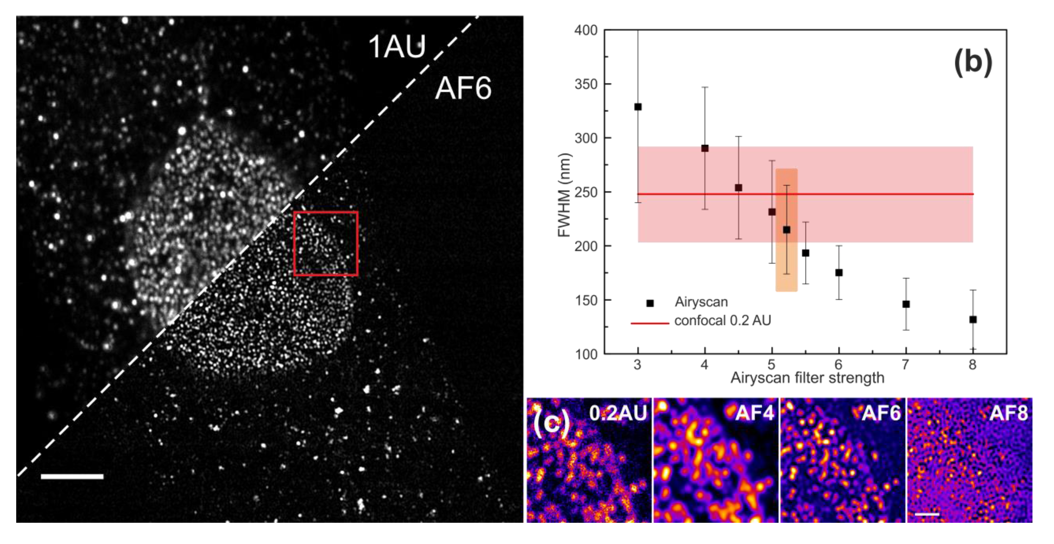
Having characterised fluorescent bead, as well as the Argo-SIM reference samples, we next sought to investigate whether the observed improvements in spatial resolution at ideal sample conditions could be translated to biological specimens. For that, we quantified the spatial resolution using the FWHM criterion by imaging the Nuclear Pore Complexes (NPC) within the cytoplasm and cellular nucleus in fixed HeLa cells with a primary antibody to Nup153 (see the Section 2) [35]. Immunostained NPCs are a very convenient biological sample for a quantitative evaluation of the lateral spatial resolution because, due to its sub-diffraction dimensions (~100 nm in outer diameter) [36], the NPCs can be used to obtain an estimate of the PSF of the microscope. Antibody-labelled NPCs have lower brightness and increased fluorescent background and a much higher labelling density, sometimes resulting in the appearance of larger spots possibly consisting of non-resolved NPC aggregates, compared to our non-biological reference samples. We found that, similarly to the bead reference sample, the FWHM of NPCs decreased with higher AFs (Figure 5a). The spatial resolution of the post-processed Airyscan images was comparable to confocal 0.2 AU (247 ± 59 nm) already at AF4.5. Even higher AFs further reduced the FWHM down to 132 ± 27 nm, but at the expense of complete image distortion (Figure 5c), suggesting that AF5 and AF6 yielded spatial resolution enhancements of 6.5–30% (231 ± 47 nm and 175 ± 25 nm, respectively).
3.4. Airyscan Imaging of Live Rat Basophilic Leukaemia Cells
Having established the performance of the Airyscan detector in fixed cells, we next acquired two-colour images of the actin cytoskeleton and the FCε-receptor (FCεR) in live Rat Basophilic Leukaemia 2HR cells. To this end, we characterised the activation process of RBL-2H3 model cells expressing LifeAct-citrine and FCεR fluorescently-tagged with SNAP-tag through clustering of FCεRs by IgE-antibody binding. This was achieved by exposing the RBL cells to microscope cover-glass coated with TNP-BSA crosslinked IgE (see the Section 2) (Figure 6). Unlike the previous cases, the greater complexity of the localization patterns of the stained structures precluded a detailed quantitative analysis of the lateral resolution for each specific channel. However, a qualitative comparison of the images re-constructed with different settings showed similar behaviour to the previous simpler image datasets (Figure 6b). Specifically, the lateral resolution was increased while the SNR was decreased for the images at 1.25 AU pinhole and the Airyscan processed with different AFs. Already at low values of AF, the SNR improvement was noticeable for processed images, as can be appreciated from individual actin filaments displayed in Figure 6b. Further improvements in the spatial resolution were again achievable by over-filtering in the image re-construction at filter setting of approximately one unit past the default settings to AF8 (Figure 6b). Even higher filtering to AF10 resulted in image distortion. Figure 6d further illustrates the increase in the noise of the actin cytoskeletal structures at high AFs, such as AF8 (red line) compared to AF7 (blue dotted line).
As mentioned in the Introduction, the Airyscan concept offers the possibility of obtaining improved spatial resolution at either enhanced or at least equivalent SNR to that of conventional confocal imaging at the 1-AU pinhole setting, while still only requiring standard laser excitation powers of a few μW. These parameters allowed live cell dynamic imaging of RBL cells for substantial time intervals at moderate loss of fluorescence due to photo-bleaching. Two colour time lapses over a total duration of 400 s with 10-s intervals experienced a loss in fluorescence of less than 5% of its original value over the total acquisition time. To this end, the results further confirmed that the Airyscan technique is suitable for live cell studies and superior to conventional confocal, because it allowed performing imaging at low illumination powers, yet achieves considerable improvement in the spatial resolution.
4. Discussion and Conclusions
The Airyscan technology has recently been introduced to bridge the gap between conventional confocal microscopy and super-resolution microscopy. This technique combines confocal imaging with a pinhole of 0.2 AU in diameter, deconvolution and the pixel-reassignment principle in order to enhance both the spatial resolution and SNR without a requirement for either greater laser excitation power or averaging of multiple images, as is often the case in conventional confocal microscopy. Consequently, Airyscan imaging is considered as a promising candidate for live cell applications. We investigated the performance of the Airyscan technology using a set of reference samples and simple biological specimens.
We demonstrated that the spatial resolution of the reconstructed Airy sum of the raw Airyscan data, which corresponds to a pinhole setting of 1.25 AU, as well as the raw data from Channel 1 of the Airyscan detector, which corresponds to a pinhole setting of about 0.2 AU, are in close agreement with the equivalent conventional confocal settings. We further found that the spatial resolution of the processed Airyscan images, for the case of 23-nm GATTA-Beads, was directly dependent on the strength of the Airyscan filter. The spatial resolution was low for AF settings less than the default setting, but improved for AFs greater than the default settings. We also found that there was only a very weak functional dependence between the image acquisition settings and the determination of the automatic Airyscan filter setting, suggesting that other factors such as the labelling density of the reference sample could contribute to the strength of the automatically-determined default filter setting. Finally, we demonstrated that the chromatic dependence on the spatial resolution of the Airyscan detector only marginally improved when using 488-nm laser excitation as opposed to 633-nm laser excitation.
Our findings further pointed out that the direct dependence between the Airyscan filter strength and the spatial resolution of a specimen holds great inherent risk for user subjectivity. Too high AFs can easily result in over-processing of the images and thus introduce feature artefacts, which can further yield false object quantifications. To overcome these challenges, new users could avoid image artefacts by imaging fluorescent beads that are larger or of comparable size at a given laser excitation to evaluate the lateral spatial resolution as a function of the Wiener filter strength. In this study, we used 200-nm diameter TetraSpeck beads and an excitation wavelength of 488 nm. There was only a weak dependence of the spatial resolution enhancement on the laser excitation power. More importantly, however, these results showed that the dependence of the spatial resolution on the AF strength was in this case asymptotic such that the values were approximately independent of the Wiener filter strength at values below the default AF setting, but the values decreased linearly at greater AF strengths, ultimately indicating that the beads were smaller than their physical specified size. This suggested that great care has to be taken if users manually adjust the AF strength.
To further investigate the performance of the Airyscan technology, we imaged an Argo-SIM fluorescent test pattern. We found that the spatial resolution and the SNR improved at default AF settings compared to confocal. Over-filtering to the AF7 setting achieved further improvements in the spatial resolution of up to 1.8-fold at similar SNR as for the case of the confocal data at 1 AU. This suggested that a reasonable compromise on the Wiener filter settings in the Airyscan re-construction process was to enhance the filter setting to approximately one unit past the default setting for an additional gain in the lateral resolution, while at the same time ensuring that the SNR remains equivalent to that of a conventional confocal image with a pinhole setting of 1 AU. Moreover, we demonstrated that in the Airyscan modality, lower illumination powers are needed to achieve good SNR compared with conventional confocal.
Finally, we tested the performance of Airyscan in fixed and live biological reference samples. First, we quantified the spatial resolution using the FWHM criterion by imaging NPCs in fixed HeLa cells. Similarly to the bead reference sample, the FWHM decreased with higher AFs. The spatial resolution of the post-processed Airyscan images was comparable to confocal 0.2 AU (247 ± 59 nm) at AF4.5, and higher AFs further reduced the FWHM down to 132 ± 27 nm, but at the expense of complete image distortion. At last, we characterised the performance of the Airyscan during the activation of live RBL cells. The greater complexity of the cytoskeletal structures precluded a detailed quantitative analysis of the spatial resolution, but the qualitative comparison indicated similar behaviour compared to the reference samples. While the spatial resolution increased, the SNR decreased for 1.25 AU confocal and the post-processed Airyscan images at different AFs. Further improvements in the spatial resolution were achieved by over-filtering in the image re-construction, resulting in image distortion. Moreover, loss in fluorescence due to photo-bleaching was minimal over the course of 1000 frames at 0.1 Hz. Consequently, these observations suggested that the Airyscan technique is superior to conventional confocal for live cell imaging, because it enables imaging at low illumination powers, while yet achieving a superior signal-to-noise ratio at enhanced spatial resolution.
Conclusively, Airyscan microscopy is therefore a promising candidate for live cell dynamical studies, but careful attention should be paid to the levels of the AF settings.
Acknowledgments
The authors express their gratitude to Esther Garcia for providing the nuclear pore complex sample. We thank the Wolfson Imaging Centre Oxford for providing microscope facility support, the Wellcome Trust (Grant Ref. 104924/14/Z/14), the Medical Research Council (Grant Number MC_UU_12010/Unit Programmes G0902418 and MC_UU_12025) and institutional funding from the University of Oxford. We thank the Wellcome Trust and the Kennedy Trust for Rheumatology Research for the Principal Research Fellowship awarded to Michael Dustin (Grant Ref. 100262/Z/12/Z) to support K.K.
Author Contributions
K.K., B.C.L. and M.F. conceived of and designed the experiments. K.K. and B.C.L. performed the experiments. K.K. and B.C.L. analysed the data. H.C.Y. wrote the analysis software. K.K., B.C.L. and M.F. wrote the paper.
Conflicts of Interest
The authors declare no conflict of interest.
References
- Godin, A.G.; Lounis, B.; Cognet, L. Super-resolution microscopy approaches for live cell imaging. Biophys. J. 2014, 107, 1777–1784. [Google Scholar] [CrossRef] [PubMed]
- Leung, B.O.; Chou, K.C. Review of super—Resolution fluorescence microscopy for biology. Appl. Spectrosc. 2011, 65, 967–980. [Google Scholar] [CrossRef] [PubMed]
- Hell, S.W. Far-Field Optical Nanoscopy. Science 2007, 316, 1153–1158. [Google Scholar] [CrossRef] [PubMed]
- Huang, B.; Babcock, H.; Zhuang, X. Breaking the Diffraction Barrier: Super-Resolution Imaging of Cells. Cell 2010, 143, 1047–1058. [Google Scholar] [CrossRef] [PubMed]
- Stephens, D.J.; Allan, V.J. Light Microscopy Techniques for Live Cell Imaging. Science 2003, 300, 82–86. [Google Scholar] [CrossRef] [PubMed]
- Fritzsche, M.; Erlenkamper, C.; Moeendarbary, E.; Charras, G.T.; Kruse, K. Actin kinetics shapes cortical network structure and mechanics. Sci. Adv. 2016, 2, e1501337. [Google Scholar] [CrossRef] [PubMed]
- Clausen, M.P.; Colin-York, H.; Schneider, F.; Eggeling, C.; Fritzsche, M. Dissecting the actin cortex density and membrane-cortex distance in living cells by super-resolution microscopy. J. Phys. D 2017, 50, 64002. [Google Scholar] [CrossRef] [PubMed]
- Schermelleh, L.; Heintzmann, R.; Leonhardt, H. A guide to super-resolution fluorescence microscopy. J. Cell Biol. 2010, 190, 165–175. [Google Scholar] [CrossRef] [PubMed]
- Li, D.; Shao, L.; Chen, B.-C.; Zhang, X.; Zhang, M.; Moses, B.; Milkie, D.E.; Beach, J.R.; Hammer, J.A.; Pasham, M.; et al. Extended-resolution structured illumination imaging of endocytic and cytoskeletal dynamics. Science 2015, 349, aab3500. [Google Scholar] [CrossRef] [PubMed]
- Wegel, E.; Göhler, A.; Lagerholm, B.C.; Wainman, A.; Uphoff, S.; Kaufmann, R.; Dobbie, I.M. Imaging cellular structures in super-resolution with SIM, STED and Localisation Microscopy: A practical comparison. Sci. Rep. 2016, 6, 27290. [Google Scholar] [CrossRef] [PubMed]
- Xu, K.; Babcock, H.P.; Zhuang, X. Dual-objective STORM reveals three-dimensional filament organization in the actin cytoskeleton. Nat. Methods 2012, 9, 185–188. [Google Scholar] [CrossRef] [PubMed]
- Betzig, E.; Patterson, G.H.; Sougrat, R.; Lindwasser, O.W.W.; Olenych, S.; Bonifacino, J.S.; Davidson, M.W.; Lippincott-Schwartz, J.; Hess, H.F. Imaging intracellular fluorescent proteins at nanometer resolution. Science 2006, 313, 1642–1645. [Google Scholar] [CrossRef] [PubMed]
- Gould, T.J.; Gunewardene, M.S.; Gudheti, M.V.; Verkhusha, V.V.; Yin, S.-R.; Gosse, J.A.; Hess, S.T. Nanoscale imaging of molecular positions and anisotropies. Nat. Methods 2008, 5, 1027–1030. [Google Scholar] [CrossRef] [PubMed]
- Vogelsang, J.; Cordes, T.; Forthmann, C.; Steinhauer, C.; Tinnefeld, P. Controlling the fluorescence of ordinary oxazine dyes for single-molecule switching and superresolution microscopy. Proc. Natl. Acad. Sci. USA 2009, 106, 8107–8112. [Google Scholar] [CrossRef] [PubMed]
- Colin-York, H.; Eggeling, C.; Fritzsche, M. Dissection of mechanical force in living cells by super-resolved traction force microscopy. Nat. Protoc. 2017, 12, 783–796. [Google Scholar] [CrossRef] [PubMed]
- Bergermann, F.; Alber, L.; Sahl, S.J.; Engelhardt, J.; Hell, S.W. 2000-fold parallelized dual-color STED fluorescence nanoscopy. Opt. Express 2015, 23, 211. [Google Scholar] [CrossRef] [PubMed]
- Hein, B.; Willig, K.I.; Hell, S.W. Stimulated emission depletion (STED) nanoscopy of a fluorescent protein-labeled organelle inside a living cell. Proc. Natl. Acad. Sci. USA 2008, 105, 14271–14276. [Google Scholar] [CrossRef] [PubMed]
- Fritzsche, M.; Li, D.; Colin-York, H.; Chang, V.T.; Moeendarbary, E.; Felce, J.H.; Sezgin, E.; Charras, G.; Betzig, E.; Eggeling, C. Self-organizing actin patterns shape membrane architecture but not cell mechanics. Nat. Commun. 2017, 8, 14347. [Google Scholar] [CrossRef] [PubMed]
- Conchello, J.-A.; Lichtman, J.W. Optical sectioning microscopy. Nat. Methods 2005, 2, 920–931. [Google Scholar] [CrossRef] [PubMed]
- Cox, G.; Sheppard, C.J.R. Practical Limits of Resolution in Confocal and Non-Linear Microscopy. Microsc. Res. Tech. 2004, 63, 18–22. [Google Scholar] [CrossRef] [PubMed]
- Cremer, C.; Masters, B.R. Resolution enhancement techniques in microscopy. Eur. Phys. J. H 2013, 38, 281–344. [Google Scholar] [CrossRef]
- Sarder, P.; Nehorai, A. Deconvolution methods for 3-D fluorescence microscopy images. IEEE Signal. Process. Mag. 2006, 23, 32–45. [Google Scholar] [CrossRef]
- De Luca, G.M.R.; Breedijk, R.M.P.; Brandt, R.A.J.; Zeelenberg, C.H.C.; de Jong, B.E.; Timmermans, W.; Azar, L.N.; Hoebe, R.A.; Stallinga, S.; Manders, E.M.M. Re-scan confocal microscopy: Scanning twice for better resolution. Biomed. Opt. Express 2013, 4, 2644. [Google Scholar] [CrossRef] [PubMed]
- Heintzmann, R.; Sarafis, V.; Munroe, P.; Nailon, J.; Hanley, Q.S.; Jovin, T.M. Resolution enhancement by subtraction of confocal signals taken at different pinhole sizes. Micron 2003, 34, 293–300. [Google Scholar] [CrossRef]
- Korobchevskaya, K.; Peres, C.; Li, Z.; Antipov, A.; Sheppard, C.J.R.; Diaspro, A.; Bianchini, P. Intensity weighted subtraction microscopy approach for image contrast and resolution enhancement. Sci. Rep. 2016, 6. [Google Scholar] [CrossRef] [PubMed]
- Sheppard, C.J.R.; Mehta, S.B.; Heintzmann, R. Superresolution by image scanning microscopy using pixel reassignment. Opt. Lett. 2013, 38, 2889–2892. [Google Scholar] [CrossRef] [PubMed]
- Gonzalez, R.C.; Woods, R.E. Digital Image Processing; Pearson Higher Ed: Cambridge, UK, 2011; pp. 231–346. [Google Scholar]
- Sánchez-Ortiga, E.; Sheppard, C.J.R.; Saavedra, G.; Martínez-Corral, M.; Doblas, A.; Calatayud, A. Subtractive imaging in confocal scanning microscopy using a CCD camera as a detector. Opt. Lett. 2012, 37, 1280–1282. [Google Scholar] [CrossRef] [PubMed]
- Engelmann, R.; Weisshart, K. Airyscanning. G.I.T. Imaging Microsc. 2014, 3, 20–21. [Google Scholar]
- Bertero, M.; Brianzi, P.; Pike, E.R. Super-resolution in confocal scanning microscopy. Inverse Probl. 1999, 3, 195–212. [Google Scholar] [CrossRef]
- Sheppard, C.J.R. Superresolution in confocal Imaging. Optik 1988, 80, 53–54. [Google Scholar]
- Huff, J. The Airyscan detector from ZEISS: Confocal imaging with improved signal-to-noise ratio and super-resolution. Nat. Methods 2015, 12. [Google Scholar] [CrossRef]
- Sivaguru, M.; Urban, M.A.; Fried, G.; Wesseln, C.J.; Mander, L.; Punyasena, S.W. Comparative performance of airyscan and structured illumination superresolution microscopy in the study of the surface texture and 3D shape of pollen. Microsc. Res. Tech. 2016. [Google Scholar] [CrossRef] [PubMed]
- Ball, G.; Demmerle, J.; Kaufmann, R.; Davis, I.; Dobbie, I.M.; Schermelleh, L. SIMcheck: A Toolbox for Successful Super-resolution Structured Illumination Microscopy. Sci. Rep. 2015, 5, 15915. [Google Scholar] [CrossRef] [PubMed]
- Walther, T.C.; Fornerod, M.; Pickersgill, H.; Goldberg, M.; Allen, T.D.; Mattaj, I.W. The nucleoporin Nup153 is required for nuclear pore basket formation, nuclear pore complex anchoring and import of a subset of nuclear proteins. EMBO J. 2001, 20, 5703–5714. [Google Scholar] [CrossRef] [PubMed]
- Beck, M.; Lučić, V.; Förster, F.; Baumeister, W.; Medalia, O. Snapshots of nuclear pore complexes in action captured by cryo-electron tomography. Nature 2007, 449, 611–615. [Google Scholar] [CrossRef] [PubMed]
Figure 1.
Airyscan microscope principle and configuration: (a) scheme of confocal and Airyscan detection paths; (b) 32 detection element arrangement in the Airyscan detector design; (c) representative images of a 200-nm TetraSpeck fluorescent bead aggregate acquired at 488-nm excitation for all four conditions: confocal 0.2 AU; Channel 1 of Airyscan detector; sum of the 32 channels of Airyscan detector; and Airyscan processed. Scale bar is 1 μm.
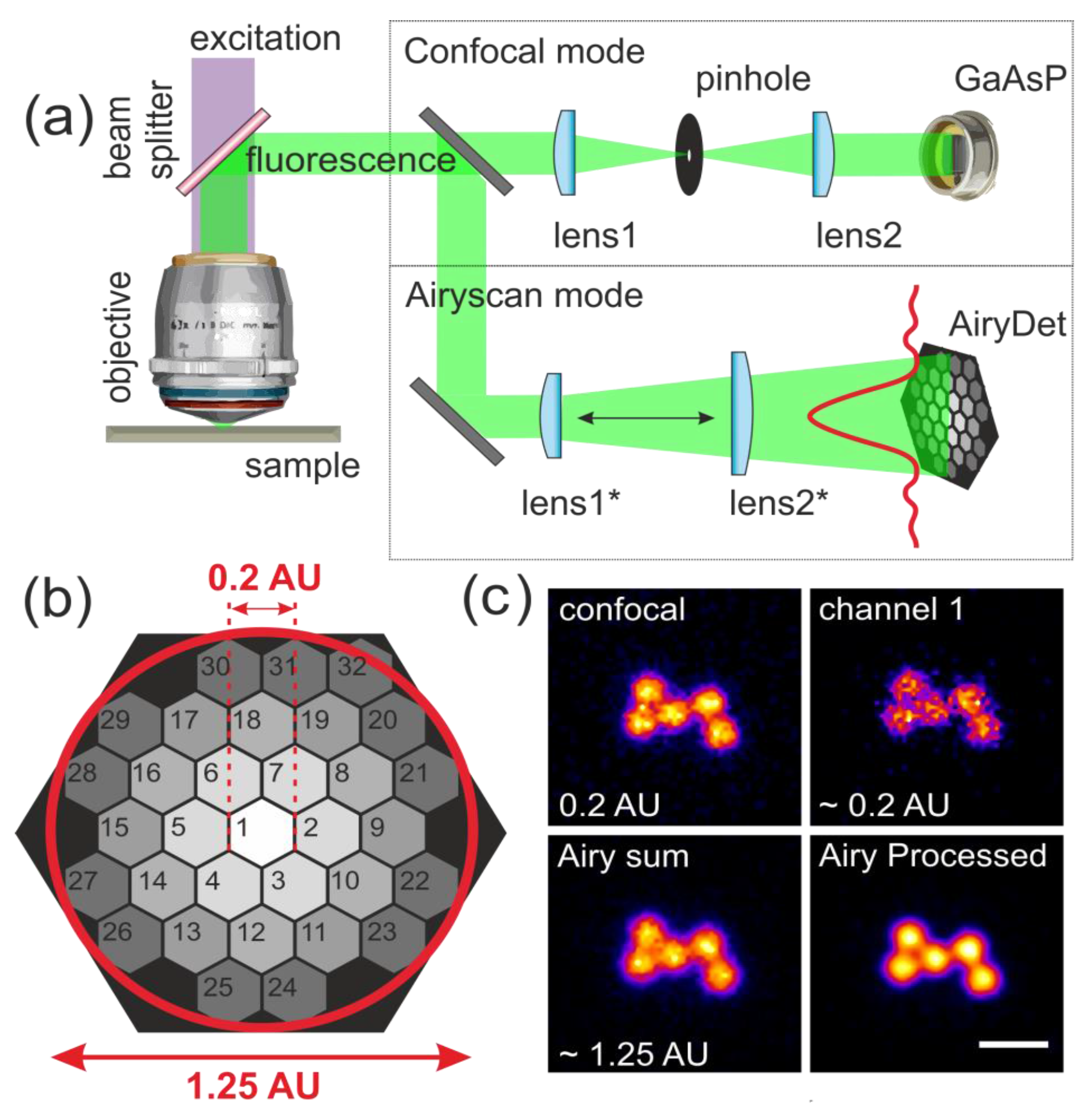
Figure 2.
Quantitative evaluation of the lateral spatial resolution by imaging fluorescent beads. (a) Representative images of the 23-nm fluorescent GATTA-Beads (OG488) in the lateral (left panel) and axial direction (right; corresponding projections along the line indicated with white triangles) acquired at 488-nm excitation, displaying all four imaging conditions: confocal using a pinhole diameter of 0.2 AU and Airyscan processed with AF4, AF6 and AF8. Scale bar is 1 μm. (b) Graph showing that the FWHM of the PSF for Atto647N GATTA-Beads imaged at 633 nm for the reconstructed Airy Sum image (open circle) and the image from Channel 1 of the Airyscan detector (open diamond) are closely equivalent to confocal images at 1 AU (open triangle) and 0.2 AU (open square), respectively. The graph further shows the strong dependence of the FWHM of the PSF on the strength of the automatically-determined default Wiener filter setting (blue diamonds) relative to the much weaker dependence (orange box) on the image acquisition settings in terms of either the excitation power (orange triangle, green diamond) or the use of line averaging (red circle, pink triangle). (c) Graph showing the FWHM of PSF vs. Airyscan filter strengths for 200 nm TetraSpeck beads (open points) imaged at different excitation powers 2, 4, 6 and 8% laser power (red, blue, black and green dots and line, respectively) and 23-nm GATTA-Beads acquired at 633-nm (black) and 488-nm (purple) excitation with 2% excitation power. Orange boxes indicate default AF settings.

Figure 3.
Qualitative evaluation of the lateral spatial resolution of Argo-SIM slide using 488-nm excitation. (a,b) Representative images of focal plane of z-stack image set of the lateral resolution test pattern on an Argo-SIM slide containing central pairs of lines with spacing gradually increased from 0 to 390 nm in steps of 30 nm from left to right. Scale bar in is 1 μm. (a) Conventional confocal image with pinhole setting of 1 Airyscan Unit (AU); and (b) processed Airyscan data at the default Airyscan Filtering (AF5.9). (c–f) ROIs (red rectangles) from (a,b) of the test pattern with specified central line spacing from left to right of 60, 90, 120, 150 and 180 nm and representative intensity line profiles from rectangular ROIs (green rectangles) with a line height of 10 pixels. (c) ROI and representative intensity line profile for confocal image at 1 AU. (d) ROI and representative intensity line profile for raw Airyscan data from Channel 1. (f) ROI and representative intensity line profile from the reconstructed sum of the raw Airyscan data. (f–j) ROIs and representative intensity line profiles for processed Airyscan data at the default Wiener filter setting of 5.9; (e) Airy sum: the sum of all 32 channels (f); and at increased Wiener filter settings of 6.5 (g), 7.0 (h), 8.0 (i) and 9.0 (j). Representative intensity line profiles in (c–j) are ROIs (blue rectangles) emphasizing the increased noise level in the case of the data from Channel 1 of the Airyscan detector only (d); and successive increase if noise level with increasing Wiener filter setting (f–j) as is also apparent in the image data in (d) and (f–j).
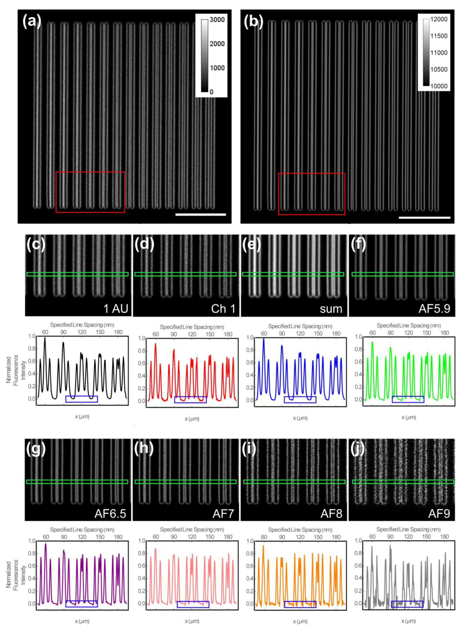
Figure 4.
Quantitative evaluation of lateral spatial resolution by imaging of the Argo-SIM slide. (a) Results from the analysis relative intensity drop, ΔI/Ipeak, for all four imaging conditions and increasing AFs as shown in Figure 3. Error bars are standard error of the mean. Also shown is the condition for the size of the intensity dip for the Rayleigh criteria for a circular aperture of ΔI/Ipeak ≈ 0.265. (b) Quantitative analysis of the SNR for all four imaging conditions and increasing AFs as shown in Figure 3. Error bars are the standard error of the mean.
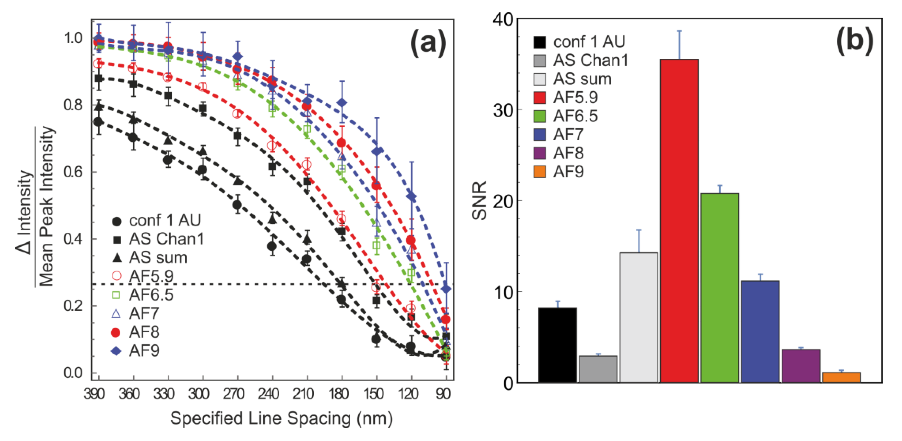
Figure 5.
Quantitative evaluation of lateral spatial resolution in biological specimen. (a) Representative image of Airy scan processed (AF6) nuclear pores complexes in fixed HeLa cell labelled by an antibody to Nup153. Scale bar is 5 μm. (b) Mean FWHM of individual NPC vs. different strengths of the Wiener filter in the reconstruction of the processed Airy scan image. The orange area shows the default filter settings; the red line shows the value for confocal 0.2 AU with the error bar (standard deviation, pink). (c) Direct comparison of the Region of Interest area (ROI; red rectangle in (a)) between confocal 0.2 AU and Airy processed images with Wiener Filters 4, 6 and 8, respectively. Scale bar is 1 μm.

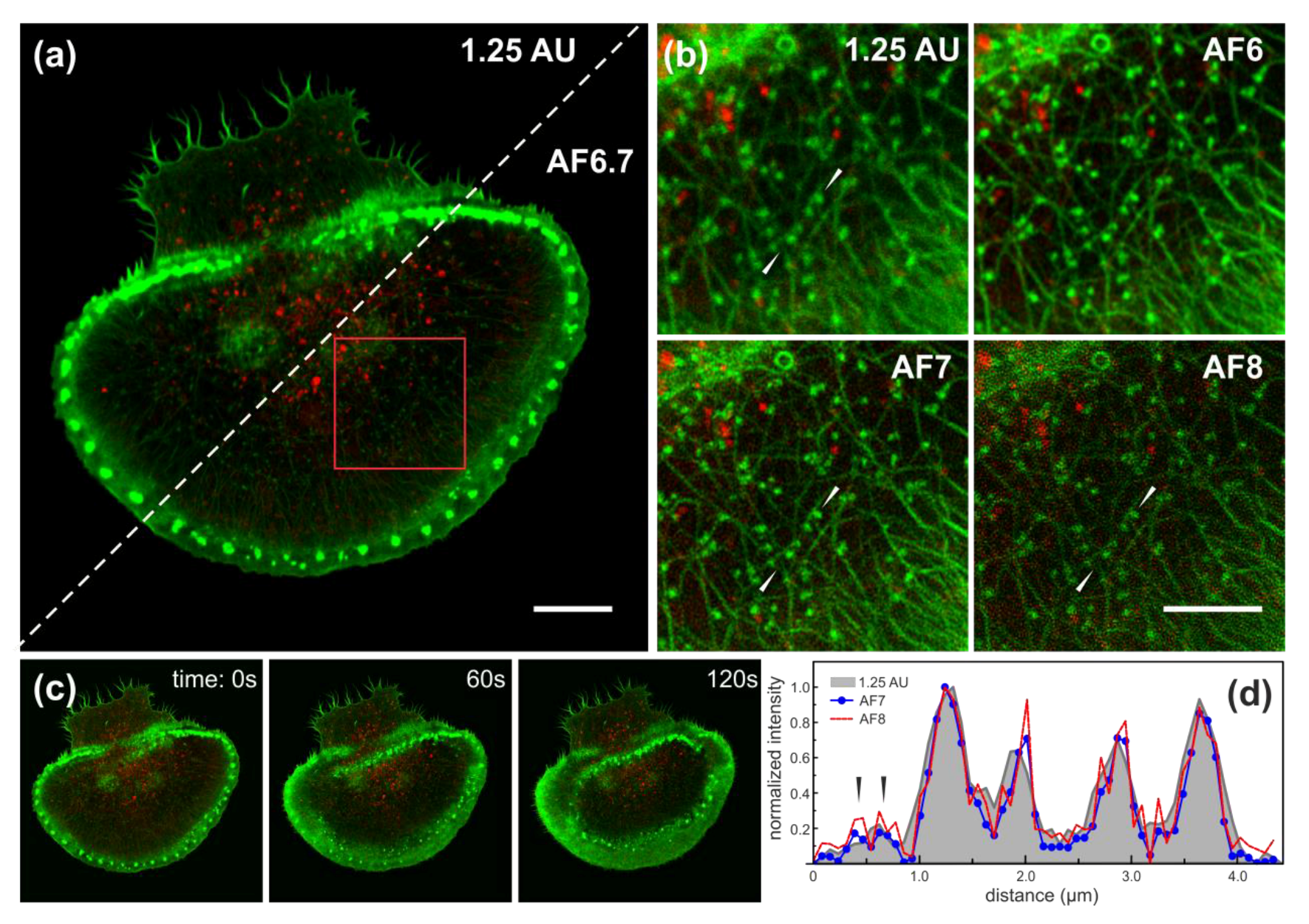
Figure 6.
Time-lapse images of activating Rat Basophilic Leukaemia (RBL) cell. (a) Comparison of 1.25 AU confocal and Airyscan processed AF6.7 images. Scale bar is 10 μm. (b) Direct comparison of Region of Interest area (ROI; red rectangle in (a)) between confocal 1.25 AU and Airy processed images with AF4, AF6 and AF7, respectively. Scale bar is 5 μm. (c) Time-lapse of activating RBL cell at 0, 60 and 120 s, respectively. Green LifeAct-citrine (excitation at 488 nm), red SNAP-tag (excitation at 561 nm). (d) Intensity profiles from 1.25 AU (grey filled), AF7 (blue dots) and AF8 (red) images along the line indicated by white arrows in (b). Arrows indicate peaks from two separate actin fibres, which are only distinguishable at high AF strength and are not resolved at 1.25 AU.

© 2017 by the authors. Licensee MDPI, Basel, Switzerland. This article is an open access article distributed under the terms and conditions of the Creative Commons Attribution (CC BY) license (http://creativecommons.org/licenses/by/4.0/).
Share and Cite
MDPI and ACS Style
Korobchevskaya, K.; Lagerholm, B.C.; Colin-York, H.; Fritzsche, M. Exploring the Potential of Airyscan Microscopy for Live Cell Imaging. Photonics 2017, 4, 41. https://doi.org/10.3390/photonics4030041
AMA Style
Korobchevskaya K, Lagerholm BC, Colin-York H, Fritzsche M. Exploring the Potential of Airyscan Microscopy for Live Cell Imaging. Photonics. 2017; 4(3):41. https://doi.org/10.3390/photonics4030041
Chicago/Turabian StyleKorobchevskaya, Kseniya, B. Christoffer Lagerholm, Huw Colin-York, and Marco Fritzsche. 2017. "Exploring the Potential of Airyscan Microscopy for Live Cell Imaging" Photonics 4, no. 3: 41. https://doi.org/10.3390/photonics4030041
Note that from the first issue of 2016, this journal uses article numbers instead of page numbers. See further details here.