Range Information Characterization of the Hokuyo UST-20LX LIDAR Sensor


1
Air Force Institute of Technology, Dayton, OH 45433, USA
2
MacB Macaulay-Brown, Inc., Dayton, OH 45433, USA
*
Author to whom correspondence should be addressed.
Photonics 2018, 5(2), 12; https://doi.org/10.3390/photonics5020012
Submission received: 19 March 2018
/
Revised: 26 April 2018
/
Accepted: 11 May 2018
/
Published: 23 May 2018
Abstract
:This paper presents a study on the data measurements that the Hokuyo UST-20LX Laser Rangefinder produces, which compiles into an overall characterization of the LiDAR sensor relative to indoor environments. The range measurements, beam divergence, angular resolution, error effect due to some common painted and wooden surfaces, and the error due to target surface orientation are analyzed. It was shown that using a statistical average of sensor measurements provides a more accurate range measurement. It was also shown that the major source of errors for the Hokuyo UST-20LX sensor was caused by something that will be referred to as “mixed pixels”. Additional error sources are target surface material, and the range relative to the sensor. The purpose of this paper was twofold: (1) to describe a series of tests that can be performed to characterize various aspects of a LIDAR system from a user perspective, and (2) present a detailed characterization of the commonly-used Hokuyo UST-20LX LIDAR sensor.
1. Introduction
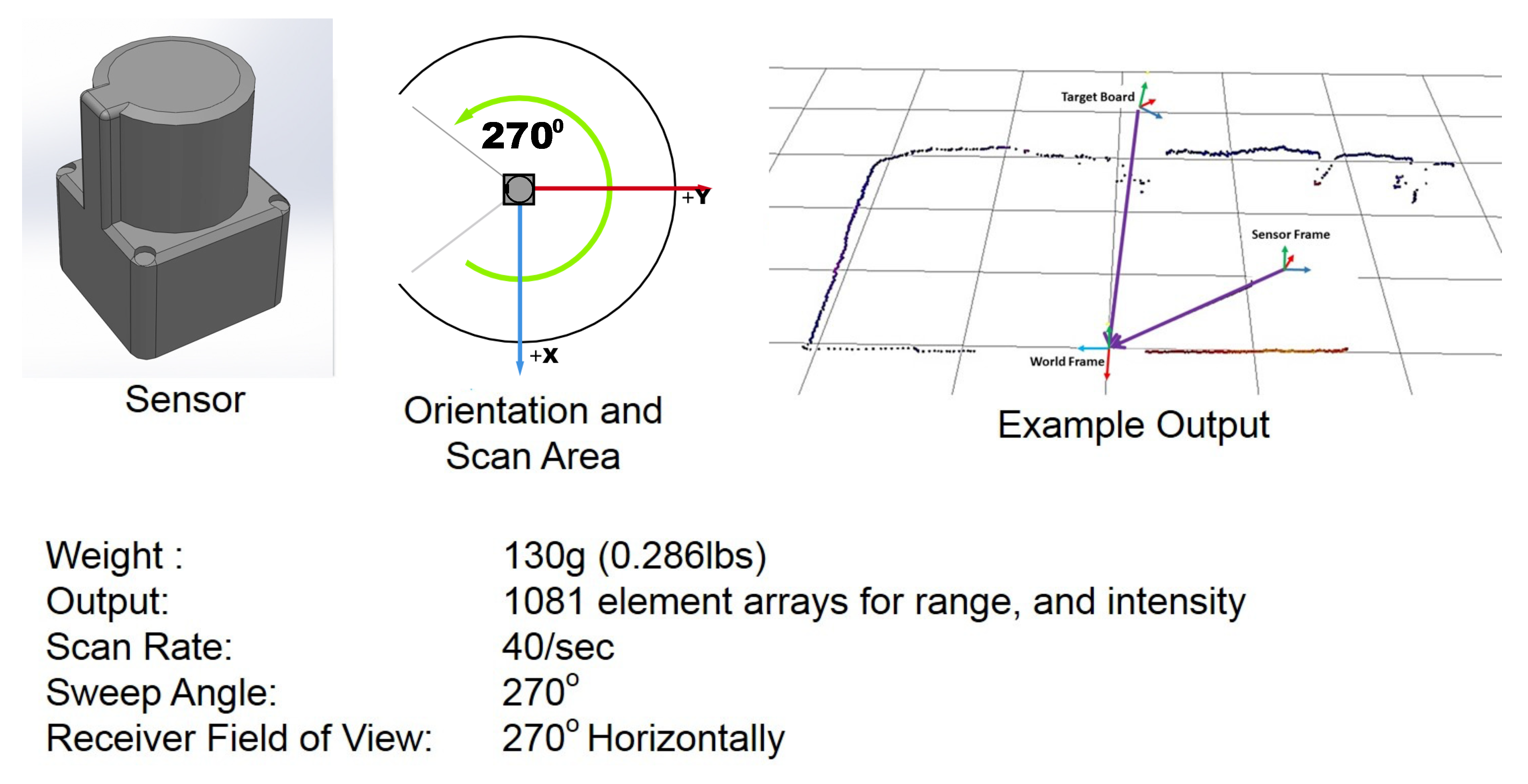
Laser Scanning Radar or Light Detection and Ranging (LiDAR) [1] sensors are a common place in the the navigation and mapping world. There are many commercial-off-the-shelf (COTS) LiDAR products for many different applications ranging from hand-held 3D mapping sensors to large 3D sensors for autonomous driving cars to even more sophisticated space-based LiDAR sensors used to monitor the health of crops across nations [2]. The LiDAR sensor investigated in this paper was the Hokuyo UST-20LX Scanning Laser Range Finder (Hokuyo, Osaka, Japan) [3] as seen in Figure 1. The sensor summary represented in Figure 1 also illustrates the sensor’s field of regard, and the output data as a 2D planar point cloud.
LiDAR sensor calibration was an important element of sensor operation and the importance of this seemingly simple task was doubly important as LiDAR sensors are typically deemed a critical sensor in aerial agricultural evaluation, robotics, and autonomous unmanned aerial vehicle (UAV) applications. LiDAR sensors are designed to measure ranging information and provide this to the user, but the information being displayed to the user may not be the true range. According to reviews of previous small form factor LIDAR sensors, the inherent noise of a small scale LiDAR sensor can cause unexpected variations greater than 10 cm [4] in the range measurements, which may be larger than acceptable for indoor navigation and mapping applications. It was therefore necessary to characterize the sensor before real-world use. Part of this characterization process will shed light on the expected error between measured ranges with the true range, object resolution at the target range as a function of angular resolution, and the variance and standard deviation of those measurements over time. Once this data was collected, and the internal but measurable error sources are identified, then the extrinsic calibration of the sensor can take place. If one had the opportunity to perform an additional characterization step, and had access to the internal electronics of the LiDAR sensor of choice, an intrinsic calibration would be done before any other characterization tests. This type of characterization would typically occur at a production facility for the commercially available sensors used in mobile robotics.
1.1. Related Work
Intrinsic and Extrinsic calibration is critical for operations of LiDAR sensors. A thorough example of an intrinsic calibration based on a LiDAR’s design specifications using a amplitude modulated continuous wave (AMCW) laser by Adams can be seen in [5], and an improved intrinsic calibration procedure for the Velodyne LiDAR line was presented in [6]. In the case of the large format LiDAR sensor like the Velodyne, an intrinsic calibration may be able to be performed if the manufacturer has an external interface already established. Users purchasing the Hokuyo UST-20LX would not typically have access to the internal areas of the sensor to perform an intrinsic calibration without generating great risk to destroying the sensor. In the context of this paper, the internal areas refer to the internal circuitry and components of the sensor. The small form factor of the packaging does not allow for much room to attach test equipment during operation. Outside of the factory testing environment, an intrinsic calibration is not as common, whereas an extrinsic calibration can be considered essential in order to operate the sensor as part of a system. In this paper, extrinsic calibration can be split into two operational and distinct categories: pixel mapping and pixel range error.
Pixel mapping refers to the process of connecting the raw sensor data to a usable data point. This can be done in numerous ways, and can use more than one type of sensor. Some common extrinsic calibration procedures use a LiDAR-Camera procedure as outlined in [7,8,9,10], and multiple LiDAR sensors or multiple sensor views as illustrated by [11,12,13,14,15,16], of a fixed target structure for a faster extrinsic calibration prior to operations [17,18,19,20]. These scenarios require the sensors raw data to be correlated into one coherent picture. Another reason to perform an extrinsic calibration was if the sensor has been physically modified as shown in [21]. In this case, the original sensor geometry may have changed and this delta in physical geometries needs to be accounted for. Each one of the papers presented describes a procedure for mapping the raw data that is within a sensor’s frame of reference to a global frame of reference through a series of coordinate transformations. This allows the raw data to be mapped to a common-format global reference frame to be used by a mapping, localization, or navigation algorithm. These extrinsic calibration techniques do not necessarily describe a sensor’s ability, or reliability, to detect a feature within its field of view.
Pixel range error, with respect to the raw LiDAR sensor data, can seem a little abstract at first, but once explained will be clear. Pixel range error from the perspective of the LiDAR sensor is the ability to distinguish between range returns from objects that are close together, laying in front of one another, was of a non-flat orientation with respect to the sensor, or has the potential to be ranged by multiple sensor range measurements within the same scan sweep. For example: at what distance will the sensor be able to distinguish a door knob protruding from a closed door when looking at it head on? This kind of characterization may be seen within the data-sheet of a sensor model, and was done during the factory article tests. This type of extrinsic calibration is of a statistical nature and requires a Monte Carlo type of testing scenario in order to clearly see the sensor’s ability to distinguish between the previously mentioned surface disturbances and a flat surface.
A truly thorough extrinsic calibration procedure enables the statistical characterization to perform not just one subset of extrinsic calibration but both pixel mapping, and pixel range error. Okubo [4] published a characterization of a similar 2D laser rangefinder to the one used in the research presented in this article. The Hokuyo URG-04LX was characterized in an effort to determine suitability for mobile robotics applications over larger and more expensive LiDAR sensors such as those used for vehicle navigation. Okubo attempted to measure the transfer rate of the sensor output, as well as the effect of drift, surface properties, and incident angles to the sensor measurements. It was found that shiny targets such as aluminum and gold caused a variation in measured ranges between 5–9 cm, whereas matte colors and grays caused a lower variation between 2–2.5 cm. Another important aspect of the paper identified an error known as mixed pixels in the range measurements. A mixed pixel was the result of the laser beam spot landing on the edge of the target. The measured range can then become a combination of the foreground and the background, and the resultant ranged returned was between those distances. The last key takeaway from Okubo’s paper was that due to the nature of the returned measurements, it was necessary to use statistical models to map the environment using this raw LiDAR data.
1.2. LIDAR Beam Propagation
Statistical randomness applies to almost every system and operation that we deal with in our daily lives, and the field of optics has a plethora of good examples of that perceived chaos. Let us now walk through the steps of what a LiDAR sensor goes through and identify where randomness in the variables apply. We will use this walkthrough to identify important concepts of the sensor performance worth characterizing.
A LiDAR sensor’s main driver is a pumped diode LASER cavity [27] to which the goal is to excite as many photons as possible. The material used for exciting photons dictates the wavelength that the LASER operates on, which is typically crystalline in nature and those atomic structures have some random properties at the microscope level. The next step involves the mirror used to pump the LASER diode by reflecting the photons back onto the LASER diode structure. The mirror placement cannot be absolutely perfect relative to the perpendicularity to the direction of the outgoing traveling wave and therefore induces another component of randomness into the system based on that imperfect alignment, small aberrations in the mirror, and vibrations. Once excited, the photons travel away from the sensor through a time-gate which blocks and unblocks the outbound light to produce a pulse or series of pulses. The timing of the gate may be accurate to within milliseconds but the wavelength of near visible or infra-red light is much shorter than a millisecond and, because the cutoff of the light is not consistent, it may induce another source of randomness in the phase. In addition, as the electronics vary in temperature (either hot or cold), the electron flow in the circuitry is varied slightly as well, which will affect the time-gate timing as well. This collection of uncertainty gives rise to intensity fluctuation in the sensor output.
After the photons break free of the sensor, they then travel as a Gaussian-like Beam [28], towards an obstacle through a propagation medium to a potential target. The range, shape, color, and orientation of the potential target was random, unless prior knowledge was known. Due to the short ranging distances (less than 20 m) measured by the UST-20LX the atmosphere was ignored during this characterization, and deferred to a follow-on research effort.
To propagate the beam through the air, there are two routes we can take: an analytic method and an estimation using a Fast Fourier Transform (FFT). The analytic approach uses the standard Rayleigh–Sommerfield Propagation also known as the Huygens–Fresnel approach [29,30,31,32] of:
where is the phase plane of the source pupil, is the range to the target, takes into account the perpendicularity of the target with respect to the sensor plane, A is the area of the pupil plane, and dS is the surface integral of the phase plane at the target. Finally, represents the phase at the target plane, which follows that is the intensity, which can be measured by traditional optical sensors.
1.3. Operation of Sensor
The previously mentioned Hokuyo UST-20LX Scanning Laser Range Finder sensor is a small scale LiDAR sensor typically used in small autonomous vehicles and simple localization devices. It has a 270 detection sweep on a single scanning plane. With a 0.25 resolution and a 270 linear field of view (FOV), it takes 1081 measurements on each sweep of the sensor. The operational wavelength is 905 nm with a bandwidth of 10 nm centered on the operating wavelength [3]. The recommended detection range is between 6 cm to 8 m assuming a minimum of 10% diffuse reflectance from the surrounding objects in the operating environment. Using a “white kent sheet”, the detection range increases to 20 m. The advertised beam divergence is 3 milli-radians and the absolute maximum output power is rated as a Class 1 Laser Device [3]. The sweep area is segmented into 1081 segments, in order to get the 1081 potential measurements. Using the supplied interface, the sensor can be modified to only output a small section of the 1081 data points, with a minimum sweep size of two measurements.
1.4. Desired Use
One intended use of this sensor was for on an Unmanned Ariel Vehicle (UAV), more specifically a large quad-rotor helicopter 18 in in diameter in order to facilitate autonomous indoor navigation research, as shown in [21]. The LiDAR scan completes a rotation so that each scan takes ranging data from the center of the quad-rotor to the directly overhead, 90 to the right, directly underneath, and then 90 to the left in a circular direction. The operating environment was indoors with the majority of the objects being ranged against being man-made and the object structures are nearly planar, or can be represented by simple shapes. This ranging data can be used to map the surrounding as the vehicle traverses down indoor corridors. The data can also be used as an mock inertial data source to feed back the estimated position information in order to estimate the parent vehicle’s velocity and acceleration, which was important for stable operation.
The importance of this study is to understand how the Hokuyo UST-20LX LiDAR Sensor takes ranging measurements and to calculate the statistics of that data as compared to the true range, and angular displacement of targets. Once the sensor data was characterized, then it can be modeled with realistic expectations to match the live sensor data. The model will be used to test real-time position estimation algorithms to enhance the UAV controls to be evaluated based on conventional control theory [33] to more advanced nonlinear control [34,35].
2. Materials and Methods
2.1. Assumptions
In order to test the Hoyuko LiDAR sensor, it is necessary to make certain assumptions. The following assumptions were made in order to proceed:
- The sensor is classified as a Class 1 Laser Device and output power is less than 1 mW; therefore, it was safe to operate without safety equipment.
- Coherence length in the laser beam is low compared to the sensor range gate length, which minimizes speckle in the returns as seen by the sensor.
- The sensor will not be affected by local illumination levels at distances less than 20 m.
- All surfaces under test will be perpendicular, unless otherwise noted.
- The testing distances of up to 5 m will give a reasonable amount of data to characterize the sensor.
- The nominal distance for indoor operation on a UAV will be between 0.5 m to 3 m.
- The LiDAR beam is close enough to Gaussian to be able to be estimated as Gaussian.
- The intensity captured by the sensor is centered on the detector plane.
- The waist of the Gaussian beam of the source is at the source plane [36].
- Gathering 10,000 samples in each test will provide enough data to infer a statistical characterization.
- All randomness in the sensor will be captured in the test data, although they may not be separable into different sources.
- The inferred angular resolution of data is not the same as the true angular resolution of target edges.
- There will be quantization error in the range returns of the sensor measurements.
3. Results
3.1. Summary of Tests to Be Described
The basic testing set-up included the Hokuyo UST-20LX Scanning Laser Rangefinder, and flat planar target boards as inferred by Figure 2 and Figure 3. Initial test placements were positioned via the use of a 1/8 in resolution measuring tape to get a rough order of magnitude placement accuracy. As a secondary and more accurate measurement system, a VICON motion capture system (VICON, Oxford, UK) was employed to measure the actual positions of both the sensor and the target boards. This was used as the set of “truth” data for evaluating measurement accuracy. An initial run was conducted to gain an understanding of the error introduced by the VICON motion capture system at different ranges within the motion capture chamber as seen in Table 1. In this scenario, the full distance of 4.0 m was near the whole diagonal width of the square testing chamber, and the distances represent moving the target board from one corner to the opposite. It can be seen that the standard deviation changes slightly as the position in the chamber was varied. The overall standard deviation can vary up to 6 mm in the z-axis, 3.4 mm in the x-axis, and 1.6 mm in the y-axis. Considering this, the VICON data points are monitored during each of the following test scenarios. Additionally, the centroid of the target was calculated and the distance to the origin of the chamber from that centroid was calculated. It is interesting to note that the standard deviation of this distance was much lower, and it shows that the noise on each axis can be considered statistically uncorrelated, which results in that lower standard deviation value.
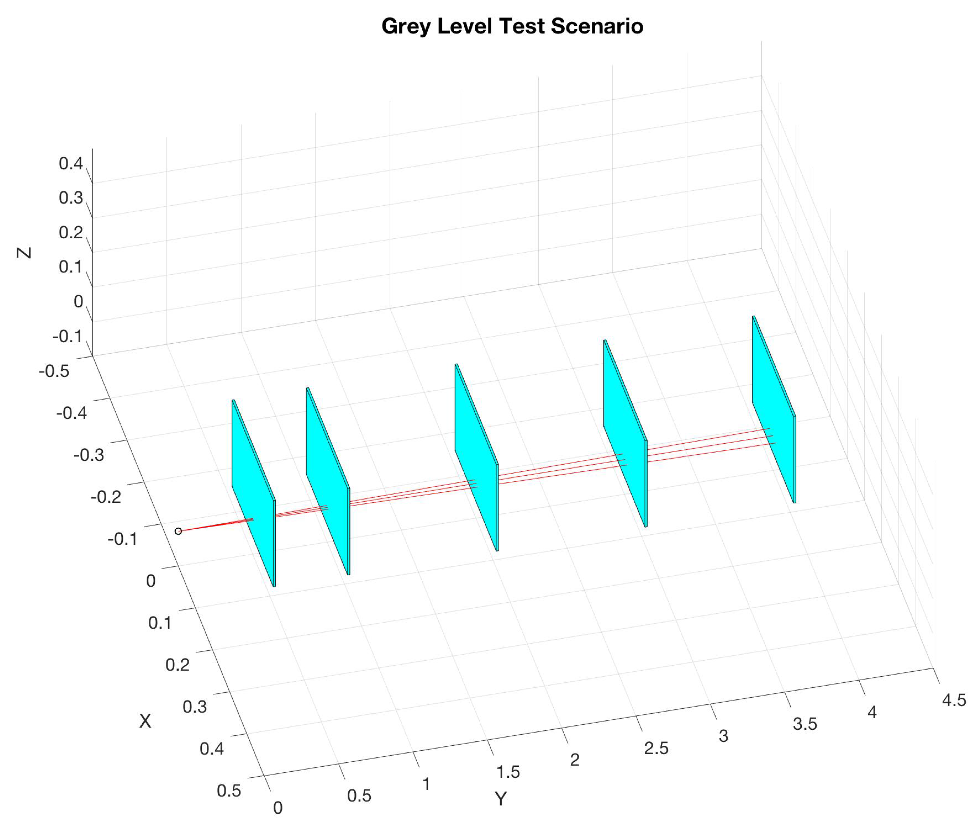
The first test, based on Figure 2, was to measure the nominal range returns across a typical range against a matte white target board. The sensor source was represented by the blue circle, the red lines represents the looking geometry of the active sensor array, and the blue squares are the locations of the target boards. The ranges to be tested were at 0.5 m, 1.0 m, 2.0 m, 3.0 m, and 4.0 m. More than 10 k data points were collected and analyzed. Once completed, a test to measure the beam divergence was conducted at ranges of 0.5 m, 1.0 m, 2.0 m, 3.0 m, and 4.0 m. From here, the next major test was the range test against a matte black and a matte white target at ranges between 1.0 m, 3.0 m, 10.0 m, and 20.0 m. Once this was completed, an investigation using a gray scale target set illustrated by Figure 4 was desired at ranges between 0.5 m, 1.0 m, and 2.0 m.
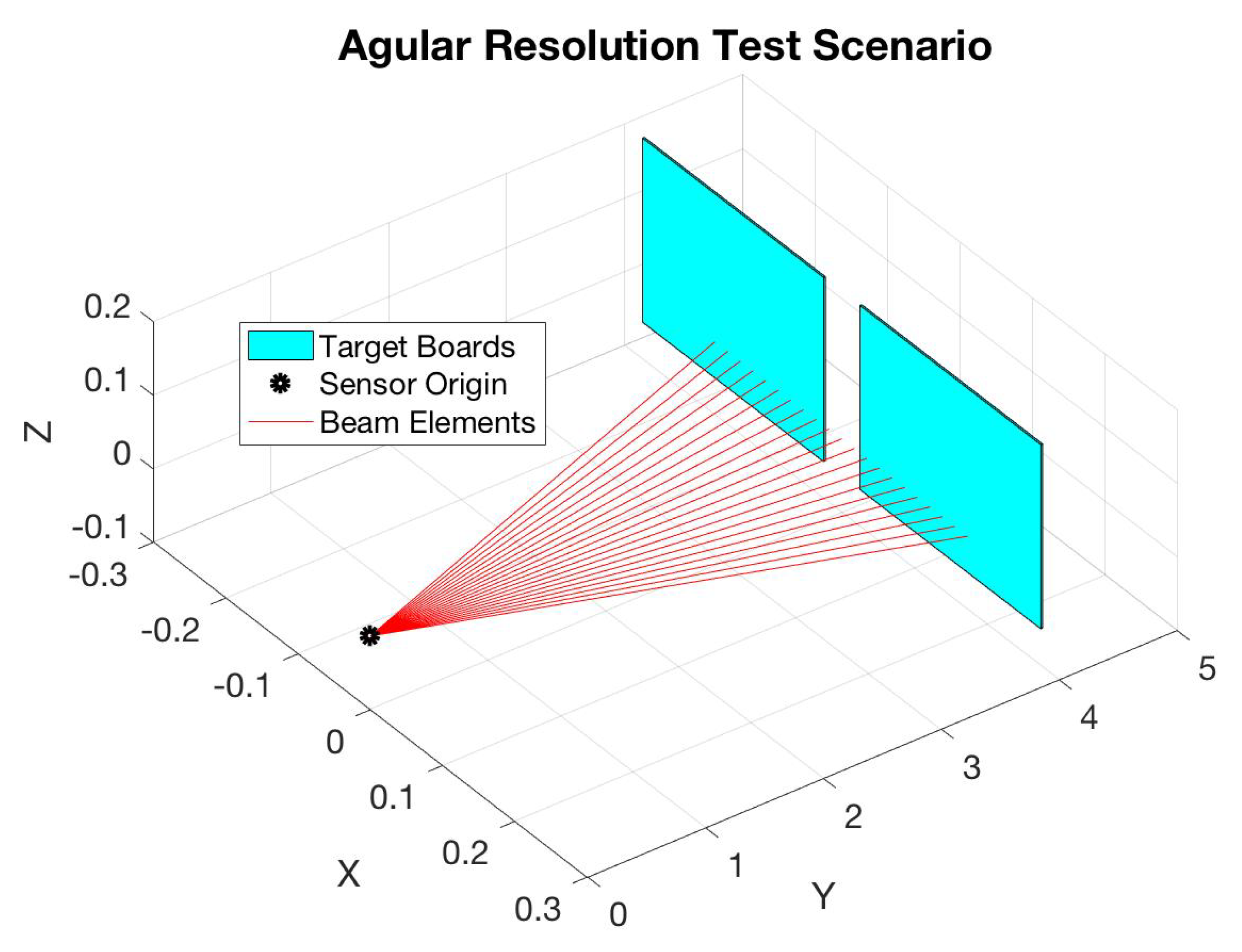
Once the basic ranging test was conducted, a test to investigate the angular resolution of the sensor was performed as shown in Figure 3. The two target boards were placed at 4.0 m and the boards were placed with such a gap between as 0.0, 1/8, 1/4, 3/8, and 1/4.
The next major test was the test to determine the amount of range error that was caused by the target’s orientation. A target board was placed at 4.0 m, and the target angle was stepped incrementally between +80 and −80.
3.2. Range Accuracy Measurements
This first test was designed to characterize the raw data range returns of the LiDAR sensor, and was the first step in identifying any potential issues pixel mapping the raw data to a usable stream. The statistical evaluation of the range returns enable a confidence in the accuracy of the measurements. This confidence may be a function of distance, and was necessary to investigate.
For this test, the sensor configured as an object within the VICON chamber, and was placed at the corner of the test chamber. The first target board was placed as close to 0.50 m according to the measuring tape, with the normal vector of the target surface point directly towards the sensor source. This can be seen in Figure 2. The target was secured into place by small weights, and then both range data and VICON measurements are taken for the three active sensor elements centered around a zenith. A minimum of 10,000 data points are collected for a reasonableness in statistical accuracy and analyzed.
The first set of range data was shown in Table 2. The data set in Table 2 shows data collected for the three center data points of the LIDAR sensor. This figure shows the mean and standard deviation (STD) of the error with respect to the measured range. Recall that propagating three beams are necessary due to the fact that the minimum beam count was two as allowed by the internal software of the sensor, and by using three active elements will allow for a more accurate estimation of the center of the center beam due to symmetry.
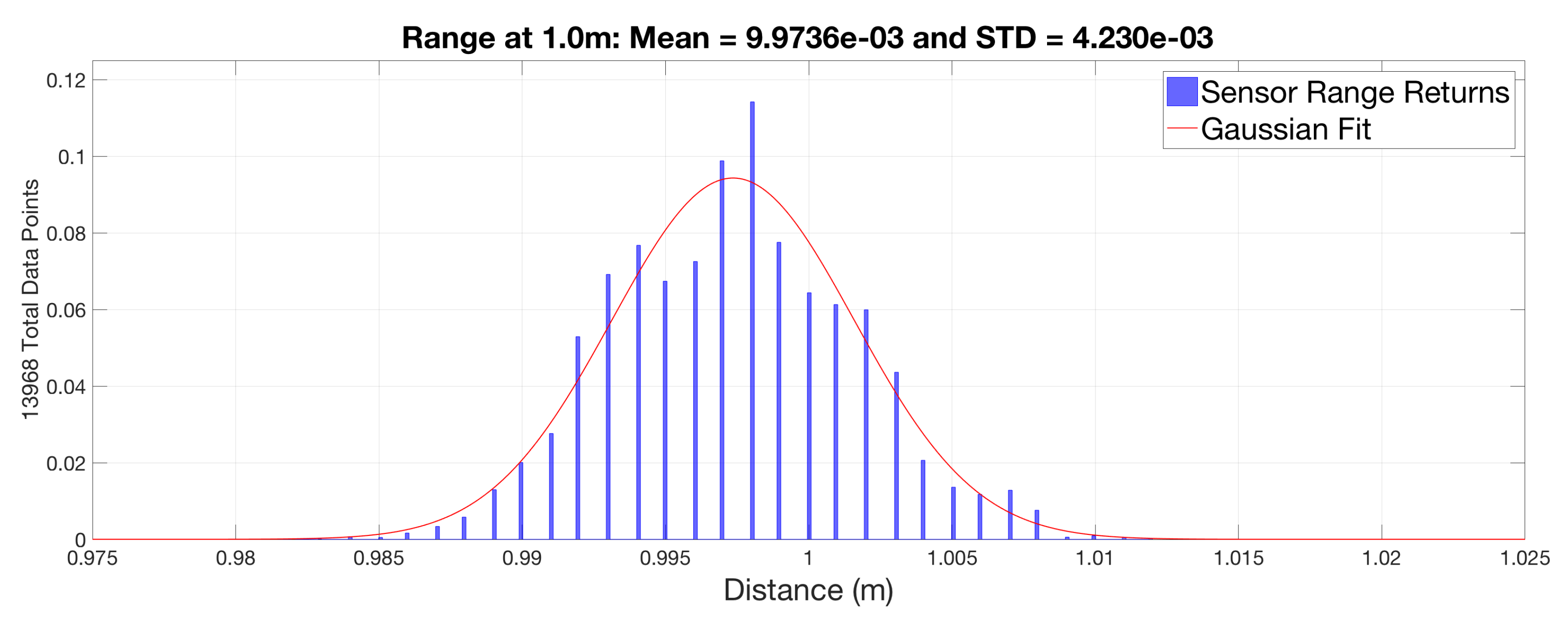
Figure 5 shows a histogram of the collected data points for the 0 sensor output at the 1.0 m distance. The actual sensor data was represented by the histogram in blue, and the Gaussian distribution pattern describing it was in red. An item of note was that the sensor gates the range return into 1 mm increments. Therefore, the natural tolerance of the sensor was mm due to the range gating of the internal electronics.
3.3. Black and White Range Measurements
In a localization and mapping environment in which typical small form factor LiDAR sensors will be utilized, a slightly neglected area was how the target interacts with the wavelength of the sensor, and of the sensor’s ranging calculations. The target’s material can essentially induce error in the range measurements due to how that interaction can change the signal-to-noise ratio (SNR) of the receiving sensor, as an initial test for the susceptibility of this on the Hokuyo sensor was to identify if a black or a white target board gives a noticeable difference in range returns. This is an interesting test case in that understanding the effect of the two extrema can provide an expected error bound for an actual real-world application that is not made up of an entirely black and white environment. There have been numerous error analysis studies on sensors of a similar concepts such as in Time-of-Flight (ToF) cameras. In these studies, the authors have used black and white checker boards to essentially average out the effect of black and white targets to provide a more “accurate” range measurement as seen in [37,38,39]. This can provide for a more accurate range estimate by the sensor, especially if included as part of a calibration stage, for operational use but does not quite investigate the error source that is desired in this paper.
The test scenario for the Range Accuracy was mimicked during this test. The significant difference in this test was that the securing weights for the target board are marked to indicate position for each distance under test to ensure that a black target board was as closely located to the same position as the white target board was. Additionally, due to the lengths of this test, the VICON chamber was not utilized, and the test needed to be moved into an engineering hallway to secure the needed space. In this test, the measuring tape, with a 1/8 in tolerance, was the only measuring device. Due to this limitation, the distances were measured three times in each data collect. The test was limited to 20 m due to the sensor limitation at greater distances. Another run was attempted at 30 m, but the sensor returns were so weak in the ambient light that the accuracy of the range returns had to be ignored.
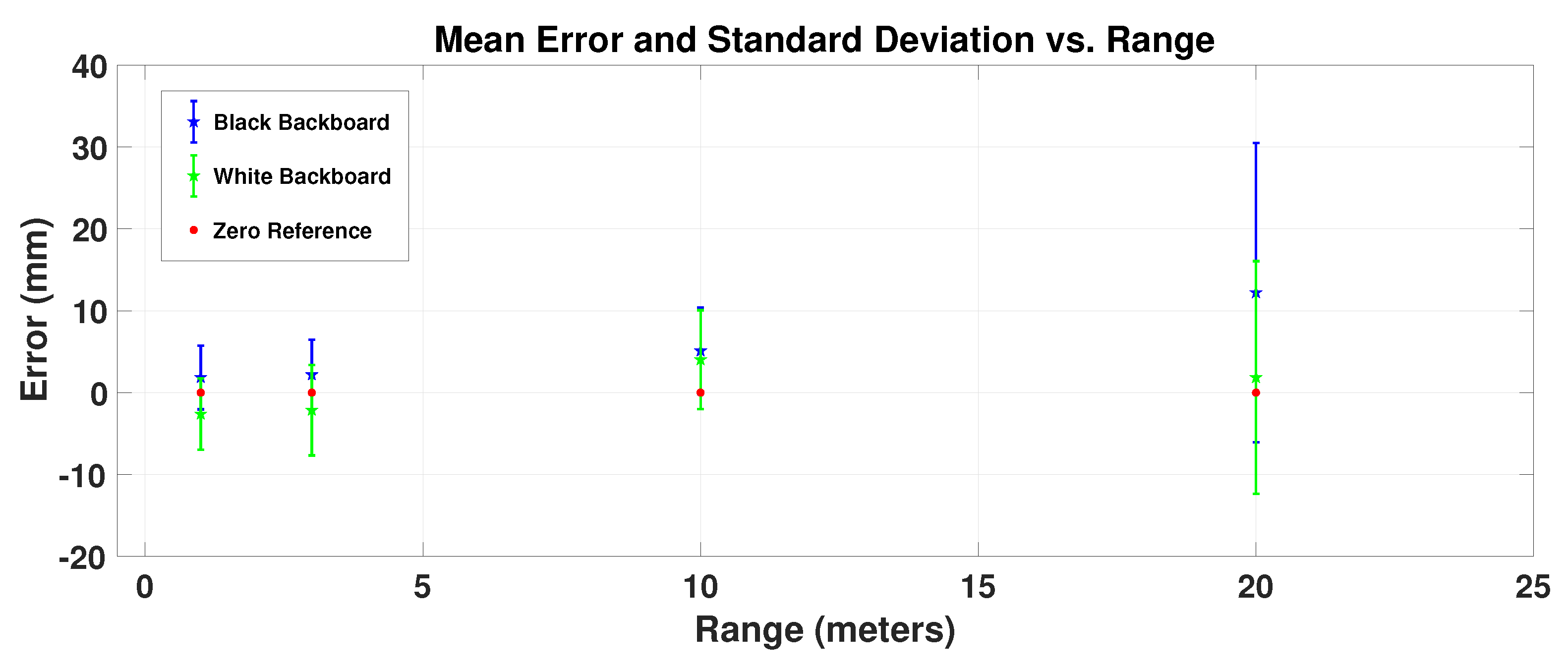
For the first scenario comparing range returns of a black or white matte board, the range accuracy was measured using at least 10,000 samples at each desired distance of 1 m, 3 m, 10 m, and 20 m and was illustrated in Figure 6. For this scenario, the range returns are indicated in blue for the black target board, and in green for the white target board. The red circle are added to better visualize the zero-mean reference point. Doing this allows one to notice that the white target board consistently produces shorter range returns than the black target board. At shorter distances of 1 m and 3 m, the average range return seems to straddle the zero-mean reference. At a target distance of 10 m and 20 m, the mean error increases globally for both the black and white targets. The standard deviation at each test point was illustrated in Figure 6 by the vertical error bars. The magnitude of the standard deviation seems to be constant until the test point at 20 m, where it has almost quadrupled in magnitude. It was suspected that there was a point between 10 m and 20 m where the standard deviation begins to increase from a seemingly constant value for distances below 10 m.
It was suspected that the lower intensity returns, and therefore lower SNR, from the matte black board fails to trigger the threshold based sensor return at longer distances [40]. This may be the reason why the returns have a consistently longer measured distance when compared to a white matte target board.
3.4. Gray Level Test
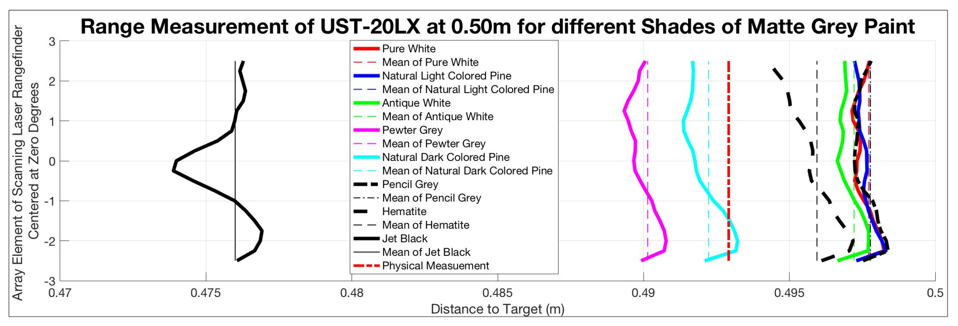
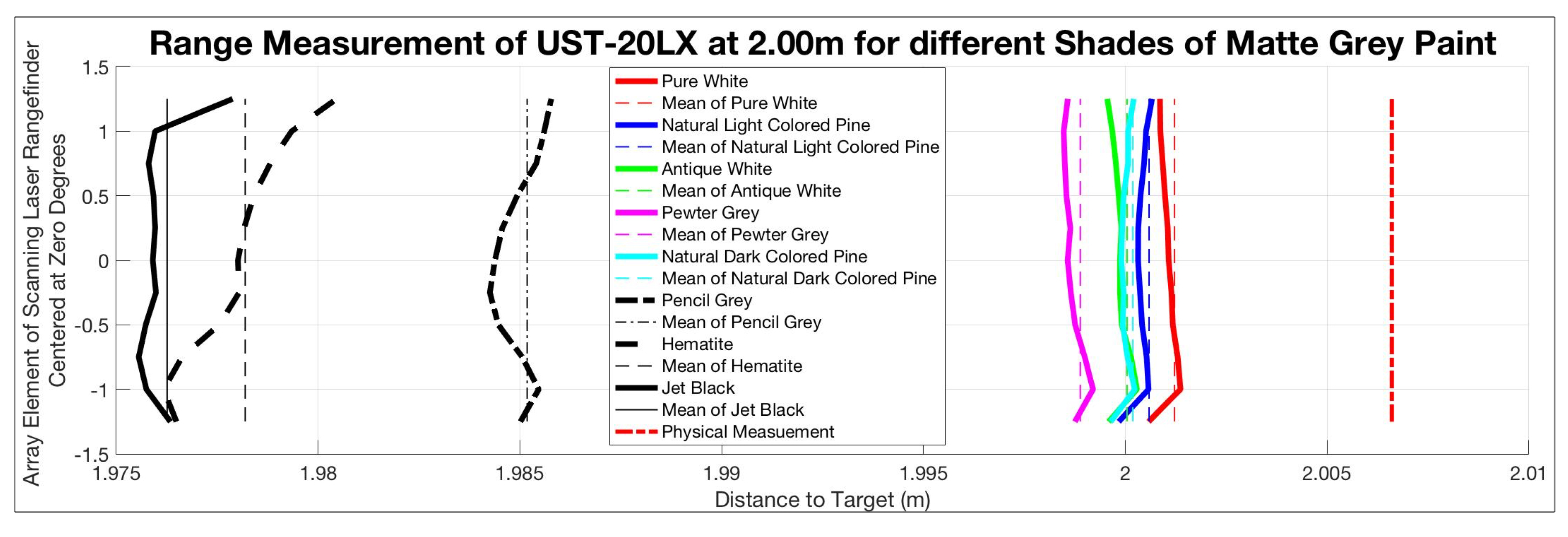
Once the comparison between matte black and matte white targets were analyzed, an additional gray level test was desired to better characterize the effects of target gray level on range error. All of the colors chosen were of the same Sherwin-Williams water-based interior latex paint line. Figure 4 represents the gray variation in painted targets. The illustration presented is an uncalibrated color image of the actual boards used, and is only included to give the reader an idea on the breadth of the grayscale colors used in this test. For reference, the darkest color is Jet Black and is shown on the far right, whereas the lightest color is Pure White and is seen on the far left. This test was conducted in almost the same exact fashion as the first Range Accuracy test. The only difference was that the target boards are slightly smaller than the original white and black target boards, due to logistical reasons. This also allows for a more secure setting for the target placement within the VICON chamber. This also ensured that consistent placement as the six painted targets and two bare wood targets were put into place for each data collect.
The results can be seen in Figure 7, Figure 8 and Figure 9. During this test, there was an anomaly at a test range of 1.5 m so the data for that distance was collected at 1.6 m and was annotated in Figure 9b. For this scenario, the test began with the pure white target board and that distance was used as the baseline for the remainder of the series. For example, the test at 0.50 m was started by placing the pure white target board in position as indicated by the thick solid red line. The range data was then taken, and the remainder of the targets were placed in the same exact location. The error in the range was with respect to the solid red line.
When analyzing the four test ranges as depicted in Figure 7, Figure 8 and Figure 9, it can be seen that the test at 0.50 m shows a different level of error. Figure 8 and Figure 9a show an actual target distance greater than any range return, whereas the test at 0.50 m shows the actual target distance in the middle of the set of measured ranges.
3.5. Beam Divergence
Once an understanding of how the target color effects the range return, a test to measure the beam divergence was necessary. The beam divergence of the LiDAR sensor was an important characteristic because this phenomena can play an important part in the usability of the sensor in terms of pixel range error. For this test, the common test scenario in measuring the Range Accuracy, and of the errors caused by different gray levels of the target, was used once again. In this version of the test scene, only the matte white target board was used at each target distance. For each distance, a three-element pattern was used, and the target was placed such that the LiDAR beam lands on the center of the target. At this point, an infra-red optic was used to “see” the beam spot as it landed on the target and was traced out by hand onto a small piece of paper placed at the same location. The traced image was then measured via metric ruler with a tolerance of ±0.5 mm. This step was repeated twice at each target distance to help ensure a consistent measure.
The beam spot size on target can play into a number of different error sources. The first error type was a “Mixed Pixel” as described by [4]. A mixed pixel represents a range return where the sensor has illuminated multiple different targets at different distance planes. The results of this can be seen more in the Angular Resolution test discussed in the following section. Beam spot size can also introduce error due to the target orientation, as the LiDAR return may not follow a traditional Gaussian shaped return. The return may in fact be skewed due the target orientation with a closer edge of the target giving a strong enough return to trigger the sensor threshold but give an incorrect range return. This will be illustrated in the Angle Test section later.
Table 3 shows the beam spot size measurement using the three-beam pattern previously discussed. It can be seen that the “width” of the beam spot was proportionally much larger than the “height" of the beam. Combining this data with a difference equation in Equation (2) gives an average beam divergence of 0.413 mRad by 17.23 mRad. This divergence ration gives a little insight into the construction of the laser source. It would appear that vertical edges encounter stronger spatial filtering, whereas the horizontal edges do not. This spatial filtering creates a beam spot size that was disproportional, and can help visualize the difficulties in detecting features at long (greater than 2.0 m) distances:
where was the angle of divergence, h(n) was the height at the nth distance, and d(n) was the n-th distance. was the average angle of divergence in the vertical direction and was the average angle of divergence in the horizontal direction.
3.6. Angular Resolution Measurements
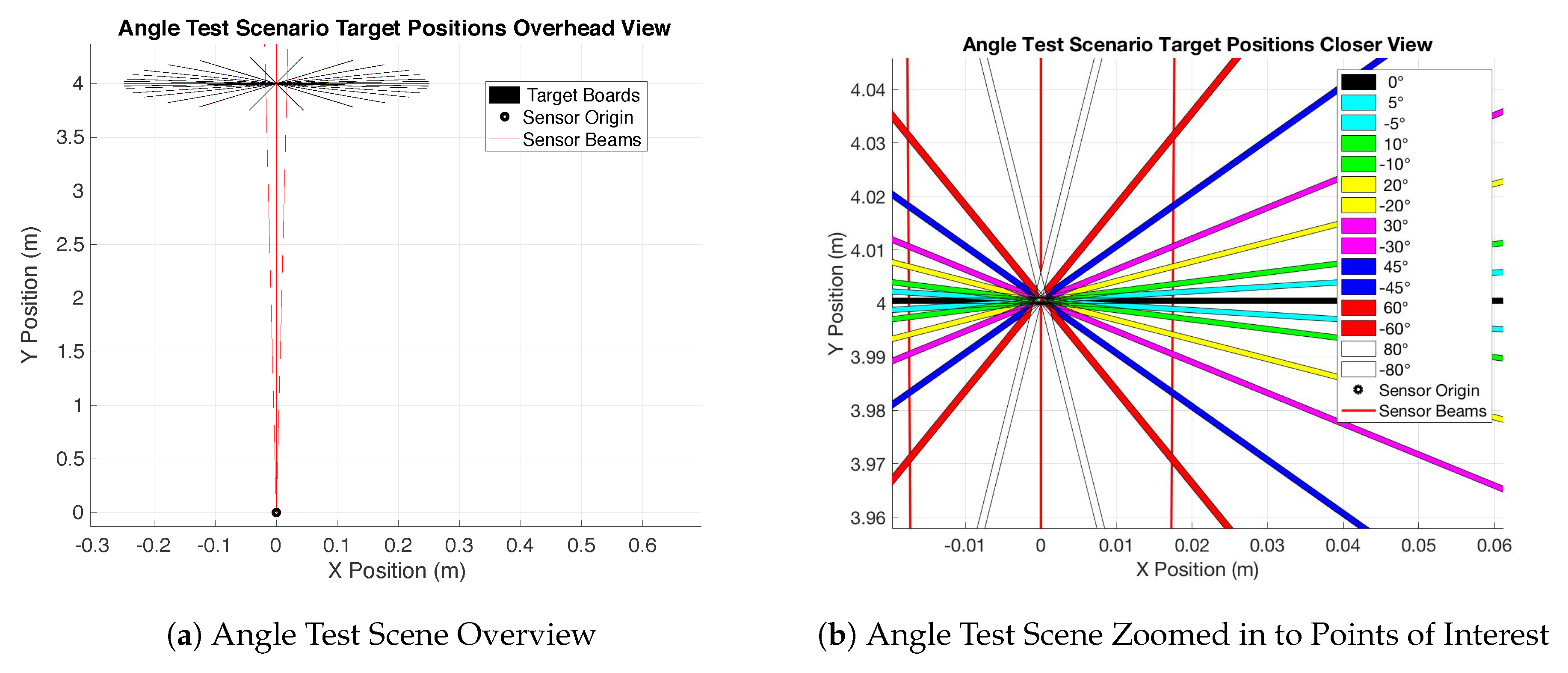
Continuing to investigate the pixel range error capability from the beam divergence test previously conducted, the angular resolution test was performed. The generalized test scenario can be represented by Figure 3. Here, the sensor is placed at the black dot in Figure 3 representing the sensor origin. From here, two matte white target boards are placed such that they share the same orientation, with the collective target set normal vector pointing back to the sensor origin. This creates a perpendicular “impact” point for the LiDAR sensor’s photons. The target distances measured are at 3.0 m and 10.0 m. This distance did not allow for use of the truth data garnered through the VICON chamber and distances were again measured solely via a tape measure. This measurement was performed three times each such that reasonable accuracy was performed. The goal of this test was not to evaluate distance, as such the accuracy of the distance was not extremely critical, but rather to characterize effects near those representative distances and to identify how small a feature can be to be detected with a reasonable confidence. Once the test was set-up, initial data collect is performed for a baseline. Then, the target boards are adjusted laterally such that a 1/8 gap now appears between them with respect to the sensor origin. This is repeated in 1/8 increments to 1/2. Each data set collects at least 10 k data points. This overarching procedure is repeated again at 10 m.
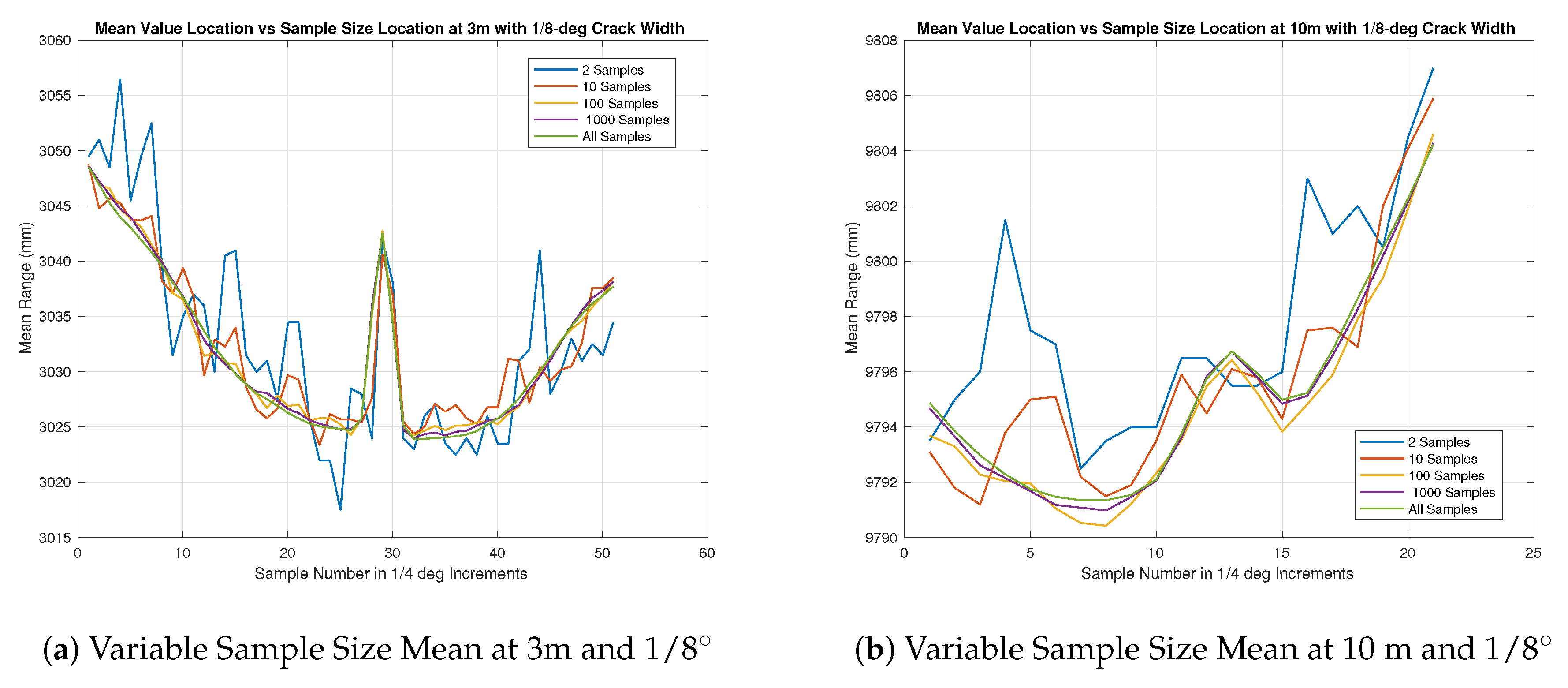
The results for the Angular Resolution test were much more challenging to determine with the collected data. During testing, the initial results to determine accurate alignment in real time was done by the UrgBenri visualization tool provided by the sensor manufacturer, Hokuyo. The resolution of the visualization tool was such that it did not show that any kind of feature was present when the hole depth of the angular gap was no deeper than 2 cm and therefore a much larger feature definition is required in order to visualize it with the UrgBenri software. In this case, both the UrgBenri software, and the raw sensor data was used. For the set of measurements in Figure 10, Figure 11, Figure 12, Figure 13 and Figure 14, the UrgBenri visualization tool did not show any gaps, but, upon looking at the mean of the collected raw data of 10 k samples, it was very evident, as seen in the summaries in Figure 10a,b. The output of the UrgBenri visualization tool did not show any relevant information not already captured in Figure 11a, Figure 12a, Figure 13a and Figure 14a and therefore is not included for simplicity’s sake. In the single sample case, it was extremely difficult to properly identify the location of the target gap. Keep in mind that the data presented here was not corrected for the range error as the angle from the norm increases, which accounts for the appearance of a “curve" in the presented charts.
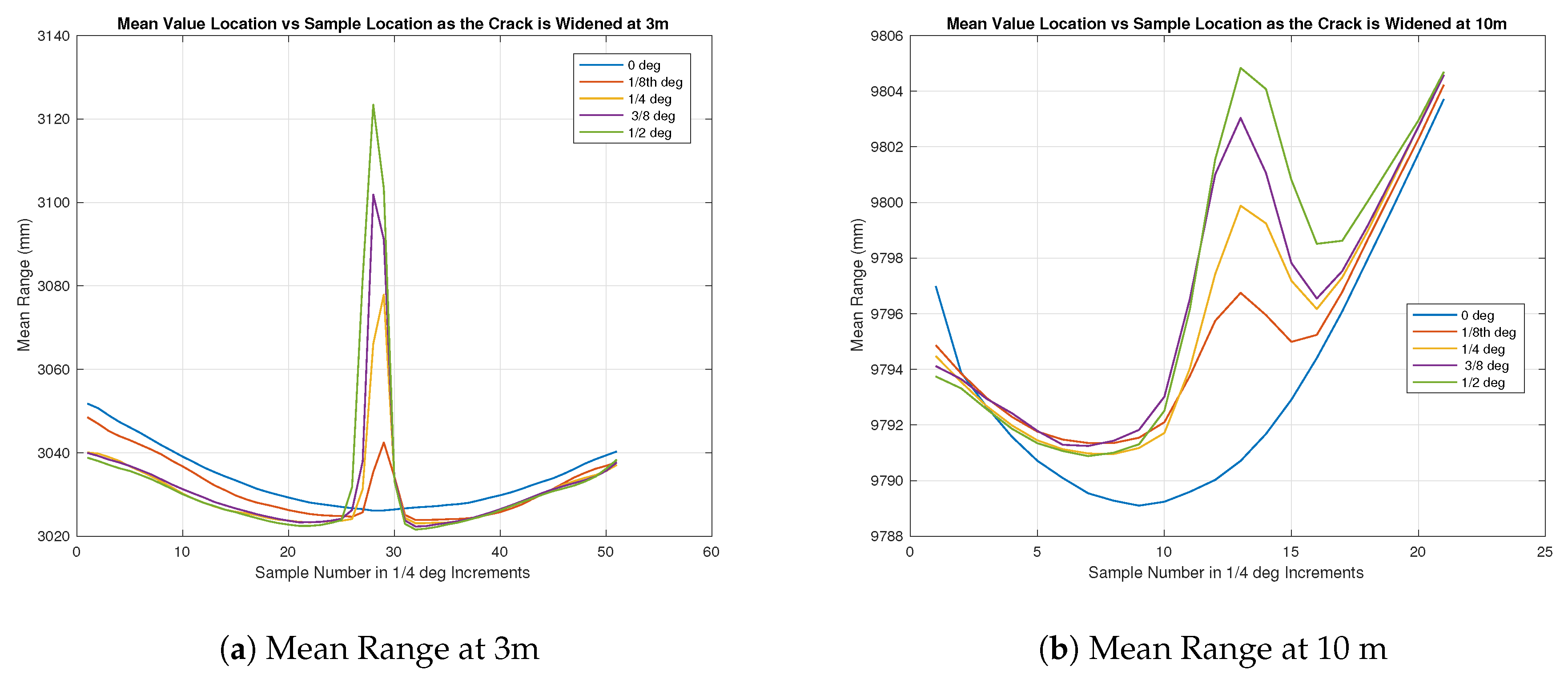
Figure 10a shows the test results at a distance of 3 m from the sensor as the gap increased according to Table 4. Across 10 k samples, the mean was taken to produce the given results and it was very apparent that there was a discontinuity in the surface when the gap was as small as 6.65 mm, even though the angular separation between the beam samples are 1/4 degrees according to the manufacturer’s specification [3].
In Figure 10b, similar results can be seen as shown in Figure 10a but across less samples overall in the figure. The gap indicated was proportionally the same size between Figure 10a,b at about 5–6 samples.
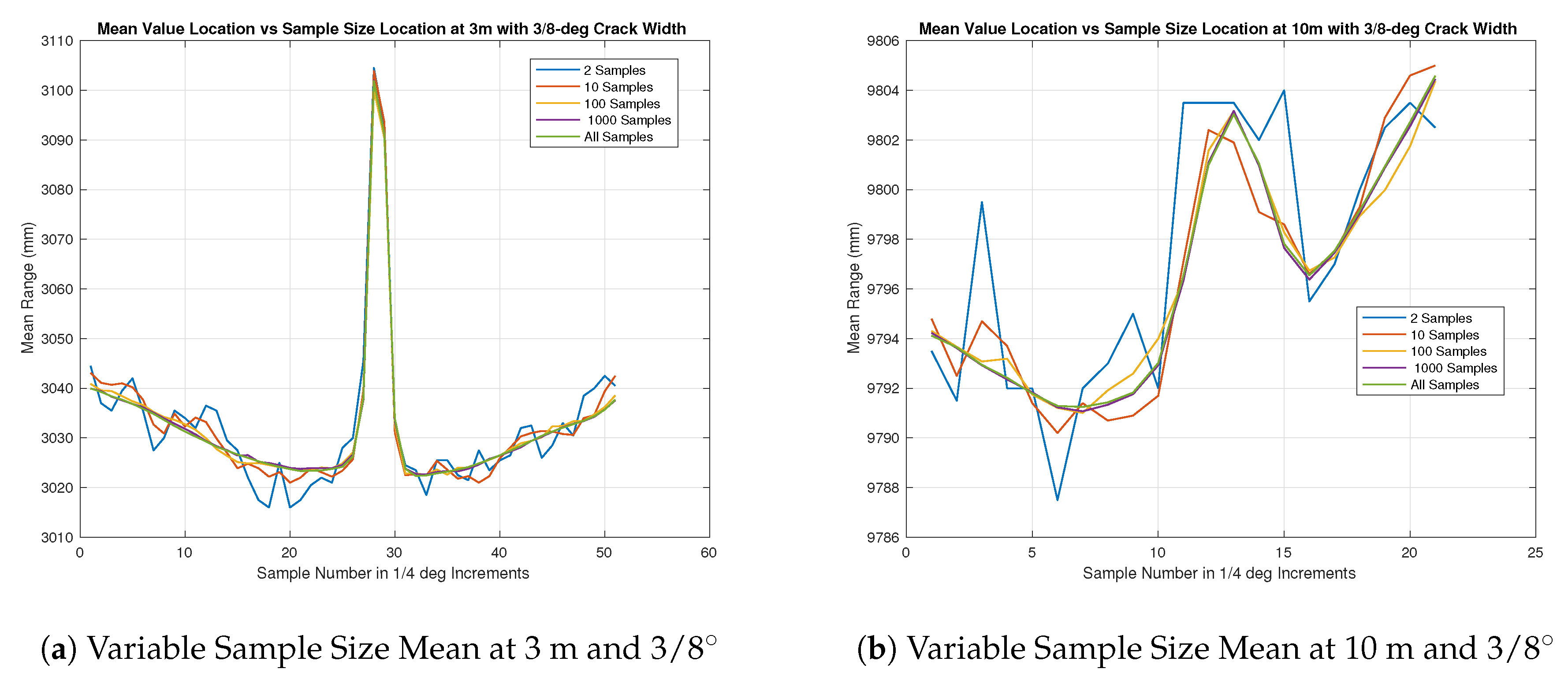
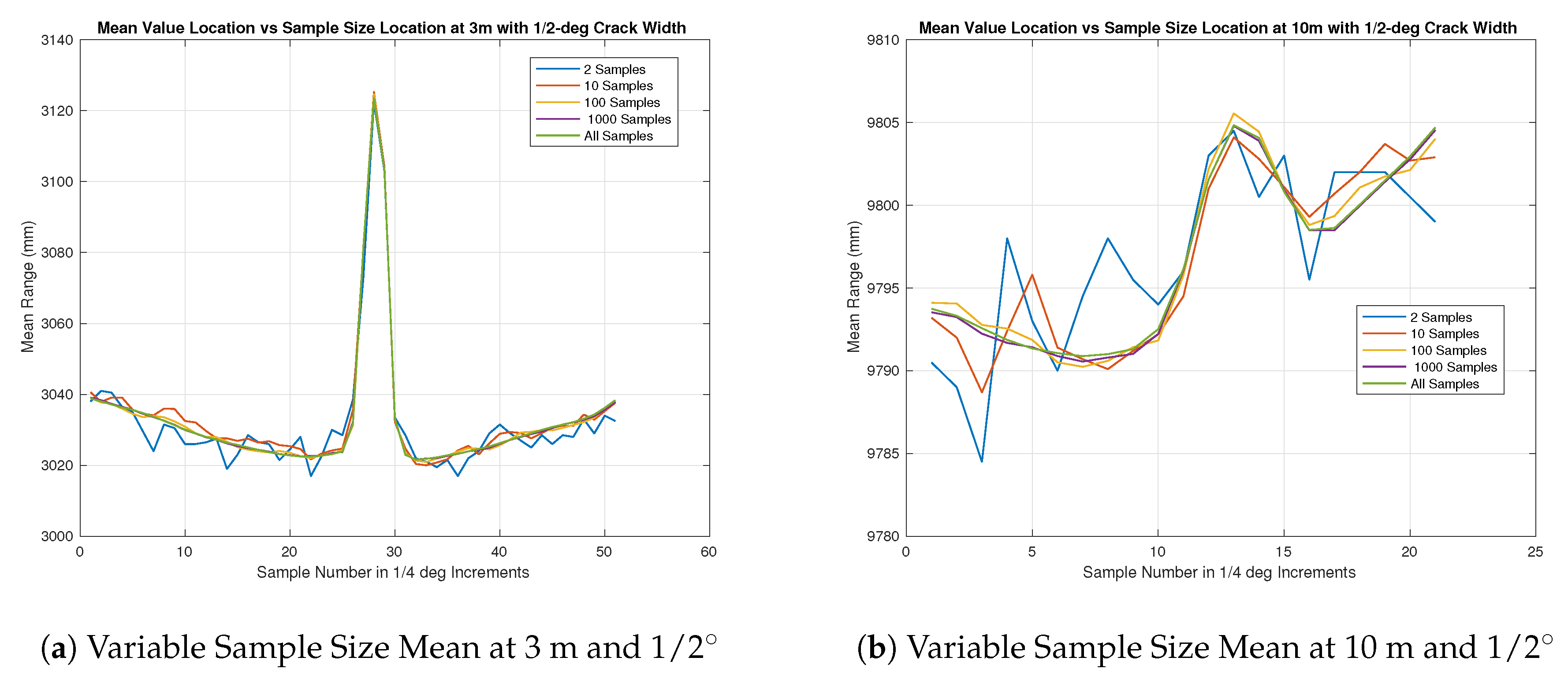
Figure 11a, Figure 12a, Figure 13a and Figure 14a show the progression of the gap size as the number of sample measurements increases. In the simplest case, using a 10-measurement mean seams plausible in all cases but for a flat surface where the variance in the return was large enough to be unclear if something was there. In the rest of the cases at a distance of 3 m, it seems that a 10-sample mean will give “good enough” results to infer that there was a hole at that location.
In all cases, it appears that the mean sample waveform, across all but ones calculated with the lowest number of samples show a constant gap width of about 5–6 sensor-beam elements. This corresponds to roughly 1–1.5 degrees. The largest sized gap under test had an angular resolution of only 1/2 degrees, which was equivalent to two sensor beam elements. With this in mind, the results appear to describe anything below 1/2 degrees as about 1.5 degrees, and it could be inferred that this will hold true as the angular distance of the gap increases. Another interesting note is the comparison between the “b” series in Figure 10, Figure 11, Figure 12, Figure 13 and Figure 14 as compared to the “a” series. In theory, the angular resolution is the same in each figure and therefore should be equal if no other factors are affecting the range returns. It can be seen that this is not the case. Combining this information with the previous insights gained through the beam divergence tests, and of the longer range black and white range test, it can be surmised that the longer distances influence the range returns. This influence has distorted the features in the target plane and causes it to be larger, but not as pronounced as it should be.
3.7. Target Angle Test
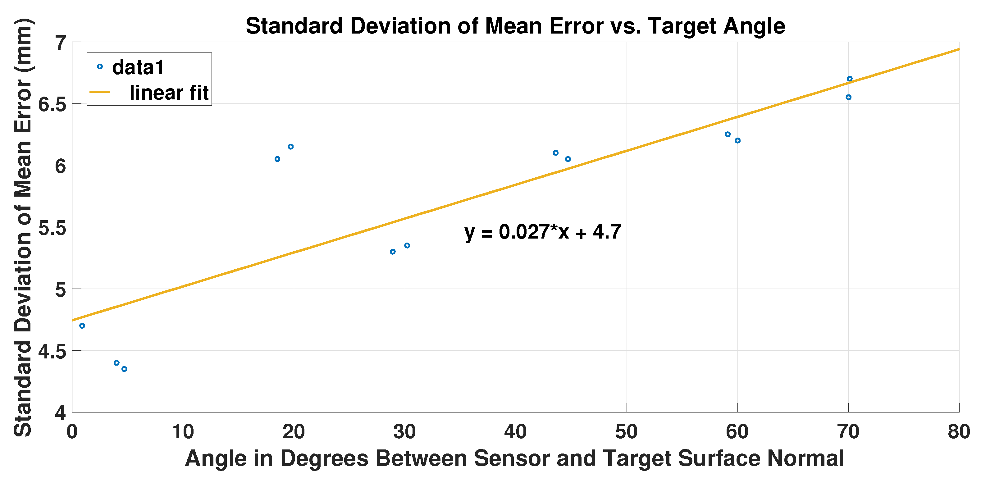
The last major test was what we are calling the target angle test. This test influences both the pixel range error and pixel mapping characteristics of the sensor. In this scenario, the LiDAR sensor is placed at the sensor origin as seen in Figure 15a. It then propagates to a white matte target board placed at 4.0 m. The goal of this test is not to evaluate a specific characteristic due to distance but of a pixel range error capability. The target distance of 4.0 m was decided, as this allowed for more room to manipulate the target into extreme orientations. This was the farthest distance that could be achieved with high confidence in the VICON range measurements, while simultaneously ensuring a large enough beam spot size to force a potential error, inducing a situation through extreme target orientation angles up to . At a closer distance, the spot size becomes smaller and can limit the error inducing potential during the test. The chosen distance also amplified the errors such that it was reasonably measurable while still being in the confines of the VICON chamber. Figure 15a,b presents the test scenario for evaluation. The target range was centered at 4.0 m, while a target board was oriented between a range of angles of as referenced in Figure 16. The goal of this test was to gain an understanding of how the beam spot size affects the range error as the orientation from beam normal was increased. Ideally, the spot size would be extremely small such that the target orientation does not affect the sensor range return.
Figure 16 illustrates how the standard deviation of the error changes with respect to the magnitude of the target’s orientation as compared to the sensor origin. As expected, the larger the orientation angle with respect to the sensor beam propagation vector, the larger the standard deviation of the range error. In this figure, a simple linear fit is used to show the general trend in order to enlighten the reader. The rough linear fit implies that there may be a an overarching standard deviation of mean error across the whole spectrum of angle in the order of about 4.5 mm. This can be largely taken into account by the range error previously discussed. If removed, then the increase in the error variance is decreased uniformly across Figure 16. Even with this potential decrease, the potential error caused by the target’s orientation can be over a half a centimeter at a range of 4 m.
3.8. Intensity-Range Profile
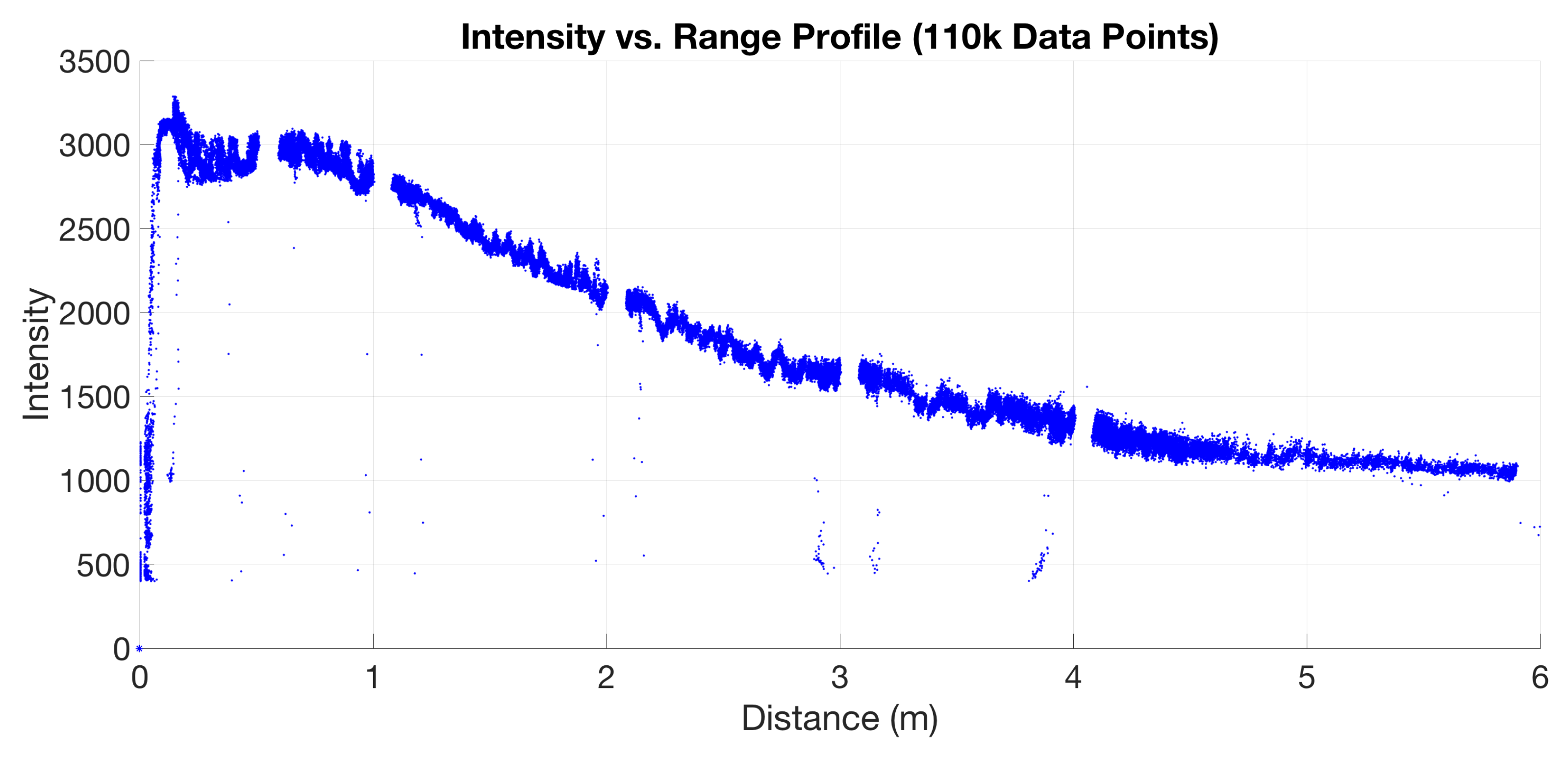
The final experiment in this characterization of the range return data of the Hokuyo UST-20LX Scanning Laser Rangefinder was an intensity profile showcasing the effect of the target distance as a function of the returned intensity. The experiment was conducted at a starting point similar to what has been referenced in many of the previous tests as seen in Figure 2. After the sensor is warmed up, a matte white target board is placed perpendicular to the sensor beam path, and then range data is collected. As the range data is collected, the target board is moved slowly along the propagation path, keeping the target board normal vector along the propagation path as well, which ensures that the sensor beam hits the flat front surface of the target board. At each meter increment (1, 2, 3, 4, 5, and 6), the target is removed from the beam path. This acts as a range check, as the voids in the collected data should coincide with the corresponding distances, as seen in Figure 17. The intensity profile seems to follow a decreasing exponential function, which may illustrate the expected SNR and the corresponding sensor threshold estimated at about 1000. For this data collection, the intensity value are in unknown units that was output by the sensor.
4. Discussion
In this paper, an investigation into the data measurements that the Hokuyo UST-20LX Laser Rangefinder produces was conducted. The first case compared the range return data to the true range across different distances over many samples. The data showed that a target range of 4.0 m produced the smallest magnitude of error within the dataset. The second and third test scenarios visualized the error caused by the color (within a gray scale). It was found that a dark target seems to consistently return a much shorter range than the actual, much more so than the other levels of the gray scale. From here, the beam divergence and angular resolution were investigated. The beam divergence was much larger in the horizontal direction with respect to the sensor orientation. It was also found that any target smaller than 1.5 in the horizontal direction may not be detectable by the sensor unless the mean of a large sample set was used for detection. Next, the target angle test was completed, which investigated the error caused by the target’s orientation. It was shown that the error was proportional to the orientation angle. The final step of the characterization was the intensity-range profile. This illustrates how range effects the return signal.
In order to minimize error sources, it is recommended to operate this sensor using a statistical average of the range returns, to operate in operational ranges between 1–4 m, and to stay away from extremely dark targets. Coupling these three recommendations together will help decrease the chances of experiencing the large error sources caused but a natural coupling of the beam divergence, and range return intensity variations.
Author Contributions
M.A.C. and J.F.R. conceived and designed the experiments; M.A.C. and R.P. performed the experiments; M.A.C. and J.F.R. analyzed the data; J.F.R. and R.P. contributed reagents/materials/analysis tools; M.A.C. wrote the paper.
Conflicts of Interest
The authors declare no conflict of interest. The views expressed in this paper are those of the authors, and do not reflect the official policy or position of the United States Air Force, Department of Defense, or U.S. Government.
References
- Bachman, C.G. Laser Radar Systems and Techniques; Artech House: Norwood, MA, USA, 1979. [Google Scholar]
- Hsu, W.C.; Shih, P.T.Y.; Chang, H.C. A Study on Factors Affecting Airborne LiDAR Penetration. Terr. Atmos. Ocean. Sci. 2015, 26, 241–251. [Google Scholar] [CrossRef]
- Hokuyo UST-20LX Scanning Laser Rangefinder. Hokuyo: Osaka, Japan, 2016. Available online: https://www.hokuyo-aut.jp/search/single.php?serial=167 (accessed on 23 May 2018).
- Okubo, Y.; Ye, C.; Borenstein, J. Characterization of the hokuyo URG-04LX laser rangefinder for mobile robot obstacle negotiation. In Proceedings of the Conference on Unmanned Systems Technology XI, Orlando, FL, USA, 13–17 April 2009; Volume 7332, p. 733212. [Google Scholar]
- Adams, M.D. Lidar design, use, and calibration concepts for correct environmental detection. IEEE Trans. Robot. Autom. 2000, 16, 753–761. [Google Scholar] [CrossRef]
- Bergelt, R.; Khan, O.; Hardt, W. Improving the Intrinsic Calibration of a Velodyne LiDAR Sensor. In Proceedings of the 2017 IEEE SENSORS, Glasgow, UK, 29 October–1 November 2017. [Google Scholar]
- Ahmad Yousef, K.; Mohd, B.; Al-Widyan, K.; Hayajneh, T. Extrinsic Calibration of Camera and 2D Laser Sensors without Overlap. Sensors 2017, 17, 2346. [Google Scholar] [CrossRef] [PubMed]
- Fuersattel, P.; Plank, C.; Maier, A.; Riess, C. Accurate laser scanner to camera calibration with application to range sensor evaluation. IPSJ Trans. Comput. Vis. Appl. 2017, 9, 21. [Google Scholar] [CrossRef]
- Kaboli, A.; Bowling, M.; Musilek, P. Bayesian Calibration for Monte Carlo Localization. In Proceedings of the National Conference on Artificial Intelligence, Boston, MA, USA, 16–20 July 2006. [Google Scholar]
- Dong, W.; Isler, V. A Novel Method for the Extrinsic Calibration of a 2-D Laser-Rangefinder and a Camera. In Proceedings of the 2017 IEEE International Conference on Robotics and Automation (ICRA), Singapore, 29 May–3 June 2017. [Google Scholar]
- Muhammad, N.; Lacroix, S. Calibration of a rotating multi-beam Lidar. In Proceedings of the 2010 IEEE/RSJ International Conference on Intelligent Robots and Systems, Taipei, Taiwan, 18–22 October 2010; pp. 5648–5653. [Google Scholar]
- Gao, C.; Spletzer, J.R. On-line calibration of multiple LIDARs on a mobile vehicle platform. In Proceedings of the 2010 IEEE International Conference on Robotics and Automation, Anchorage, AK, USA, 3–7 May 2010; pp. 279–284. [Google Scholar]
- Krotkov, E.P. Laser Range Finder Calibration for A Walking Robot; Technical Report; The Robotics Institute, Carnegie Mellon University: Pittsburgh, PA, USA, 1990. [Google Scholar]
- Underwood, J.; Hill, A.; Scheding, S. Calibration of range sensor pose on mobile platforms. In Proceedings of the 2007 IEEE/RSJ International Conference on Intelligent Robots and Systems, San Diego, CA, USA, 29 October–2 November 2007; pp. 3866–3871. [Google Scholar]
- Chen, C.Y.; Chien, H.J. On-Site Sensor Recalibration of a Spinning Multi-Beam LiDAR System Using Automatically-Detected Planar Targets. Sensors 2012, 12, 13736–13752. [Google Scholar] [CrossRef] [PubMed]
- Morales, J.; Martínez, J.; Mandow, A.; Reina, A.; Pequeño-Boter, A.; García-Cerezo, A. Boresight Calibration of Construction Misalignments for 3D Scanners Built with a 2D Laser Rangefinder Rotating on Its Optical Center. Sensors 2014, 14, 20025–20040. [Google Scholar] [CrossRef] [PubMed]
- Maddern, W.; Harrison, A.; Newman, P. Lost in Translation (and Rotation): Fast Extrinsic Calibration for 2D and 3D LIDARs. In Proceedings of the 2012 IEEE International Conference on Robotics and Automation, Saint Paul, MN, USA, 14–18 May 2012. [Google Scholar]
- Sheehan, M.; Harrison, A.; Newman, P. Automatic Self-Calibration of a Full Field-of-View 3D n-Laser Scanner. In Proceedings of the International Symposium on Experimental Robotics (ISER2010), New Delhi, India, 18–21 December 2010. [Google Scholar]
- Sheehan, M.; Harrison, A.; Newman, P. Self-calibration for a 3D laser. Int. J. Robot. Res. 2012, 31, 675–687. [Google Scholar] [CrossRef]
- Antone, M.; Friedman, Y. Fully Automated Laser Range Calibration. In Proceedings of the British Machine Vision Conference, Warwickshire, UK, 10–13 September 2007. [Google Scholar]
- Cooper, M.A. Converting a 2D Scanning LiDAR to a 3D System for Use on Quad-Rotor UAVs in Autonomous Navigation. Master’s Thesis, Air Force Institute of Technology, Fairborn, OH, USA, 2017. [Google Scholar]
- Alwan, M.; Wagner, M.B.; Wasson, G.; Sheth, P. Characterization of Infrared Range-Finder PBS-03JN for 2D Mapping. In Proceedings of the 2005 IEEE International Conference on Robotics and Automation, Barcelona, Spain, 18–22 April 2005; pp. 3936–3941. [Google Scholar]
- Kneip, L.; Tache, F.; Caprari, G.; Siegwart, R. Characterization of the Compact Hokuyo URG-04LX 2D Laser Range Scanner. In Proceedings of the 2009 IEEE International Conference on Robotics and Automation, Kobe, Japan, 12–17 May 2009; pp. 1447–1454. [Google Scholar]
- Park, C.; Kim, D.; You, B.-J.; Oh, S.-R. Characterization of the Hokuyo UBG-04LX-F01 2D Laser Rangefinder. In Proceedings of the 2010 IEEE RO-MAN, Viareggio, Italy, 13–15 September 2010; pp. 385–390. [Google Scholar]
- Pouliot, N.; Richard, P.-L.; Montambault, S. LineScout Power Line Robot: Characterization of a UST-30LX LIDAR System for Obstacle Detection. In Proceedings of the 2012 IEEE/RSJ International Conference on Intelligent Robots and Systems, Vilamoura, Portugal, 7–12 October 2012. [Google Scholar]
- Olivka, P.; Krumnikl, M.; Moravec, P.; Seidl, D. Calibration of Short Range 2D Laser Range Finder for 3D SLAM Usage. J. Sens. 2016, 2016, 13. [Google Scholar] [CrossRef]
- Jelalian, A.V. Laser Radar Systems; Artech House: Norwood, MA, USA, 1992. [Google Scholar]
- Richmond, R.D.; Cain, S.C. Direct-Detection LADAR Systems, 1st ed.; SPIE Press: Bellingham, WA, USA, 2010. [Google Scholar]
- Goodman, J.W. Introduction to Fourier Optics, 2nd ed.; McGRAW-HILL: New York, NY, USA, 2000. [Google Scholar]
- Goodman, J.W. Statistical Optics, 1st ed.; John Wiley and Sons, Inc.: Hoboken, NJ, USA, 2000. [Google Scholar]
- Max Born, E.W. Principles of Optics: Electromagnetic Theory of Propagation, Interference and Diffraction of Light, 7th ed.; Cambridge University Press: Cambridge, UK, 1999. [Google Scholar]
- Schmidt, J.D. Numerical Simulation of Optical Wave Propagation With Examples in MATLAB, 1st ed.; SPIE: Bellingham, WA, USA, 2010. [Google Scholar]
- Ogata, K. Modern Control Engineering, 4th ed.; Prentice Hall PTR: Upper Saddle River, NJ, USA, 2001. [Google Scholar]
- Sands, T. Physics-Based Control Methods. In Advances in Spacecraft Systems and Orbit Determination; Ghadawala, R., Ed.; InTech: Rijeka, Croatia, 2012; Chapter 2. [Google Scholar]
- Cooper, M.; Heidlauf, P.; Sands, T. Controlling Chaos—Forced van der Pol Equation. Mathematics 2017, 5, 70. [Google Scholar] [CrossRef]
- Milonni, P.W.; Eberly, J.H. Laser Resonators and Gaussian Beams, in Laser Physics, 1st ed.; John Wiley and Sons, Inc.: Hoboken, NJ, USA, 2010. [Google Scholar]
- Lindner, M. Calibration and Real-Time Processing of Time-of-Flight Range Data. Ph.D. Thesis, Universität Siegen, Siegen, Germany, 2010. [Google Scholar]
- Fürsattel, P.; Placht, S.; Balda, M.; Schaller, C.; Hofmann, H.; Maier, M.A.; Riess, C. A Comparative Error Analysis of Current Time-of-Flight Sensors. IEEE Trans. Comput. Imaging 2016, 2, 27–41. [Google Scholar] [CrossRef]
- He, Y.; Liang, B.; Zou, Y.; He, J.; Yang, J. Depth Errors Analysis and Correction for Time-of-Flight (ToF) Cameras. Sensors 2017, 17, 92. [Google Scholar] [CrossRef] [PubMed]
- Sup Premvuti, P.; Kirinson Inc., U.S. Official Technical Representative of Hokuyo Automatic Co., Ltd., Vancouver, WA, USA. Personal communication, 2016.
Figure 1.
Hokuyo UST-20LX sensor summary, adapted from [3].
Figure 1.
Hokuyo UST-20LX sensor summary, adapted from [3].

Figure 2.
Illustration of target positions for the variable range based tests relative to laser source.
Figure 2.
Illustration of target positions for the variable range based tests relative to laser source.

Figure 3.
Illustration of target set-up for the angular resolution test relative to laser source.

Figure 4.
Gray level test target colors.

Figure 5.
Example range return compared to the true range (meters) in a histogram.

Figure 6.
Means of 10,000 measurements at ranges between 1 m and 20 m.

Figure 7.
Gray level results at 0.5 m.

Figure 8.
Gray level results at 2 m.

Figure 9.
Gray Level Results at 1.0 m and 1.6 m.

Figure 10.
Angular resolution summary results: mean range using 10,000 sample sweeps stepping up to a gap of .
Figure 10.
Angular resolution summary results: mean range using 10,000 sample sweeps stepping up to a gap of .

Figure 11.
Comparison of angular resolution results between 3 m & 10 m range at a gap of .

Figure 12.
Comparison of angular resolution results between 3 m & 10 m range at a gap of .

Figure 13.
Comparison of Angular Resolution Results between 3 m & 10 m range at a Gap of .

Figure 14.
Comparison of angular resolution results between 3 m & 10 m range at a gap of .

Figure 15.
Illustration of the target angle test scene.

Figure 16.
Standard deviation of range w.r.t. angle test.

Figure 17.
Range return intensity profile.


Table 1.
Standard deviation of target boards at varying distances on three axes.
| Standard Deviation (mm) | ||||
|---|---|---|---|---|
| Distance (m) | X | Y | Z | Distance to Origin |
| 0.50 m | 0.45 mm | 0.19 mm | 0.41 mm | 0.19 mm |
| 1.00 m | 1.21 mm | 1.60 mm | 3.65 mm | 0.21 mm |
| 2.00 m | 1.25 mm | 1.36 mm | 5.62 mm | 0.21 mm |
| 3.00 m | 2.29 mm | 0.64 mm | 4.60 mm | 0.22 mm |
| 4.00 m | 3.39 mm | 0.81 mm | 5.91 mm | 0.46 mm |
Table 2.
Mean error and standard deviation from measured range in millimeters.
| Zenith Offset | Range | |||||||||
|---|---|---|---|---|---|---|---|---|---|---|
| 0.50 m | 1.00 m | 2.00 m | 3.00 m | 4.00 m | ||||||
| Mean | STD | Mean | STD | Mean | STD | Mean | STD | Mean | STD | |
| −0.25 | −1.7 | 4.1 | 4.4 | 4.3 | 7.0 | 3.8 | 3.2 | 4.3 | 0.8 | 4.7 |
| 0.0 | −3.2 | 4.1 | 2.6 | 4.2 | 5.8 | 3.9 | 2.0 | 4.2 | −0.4 | 4.6 |
| +0.25 | −3.6 | 4.2 | 1.9 | 4.2 | 5.4 | 3.9 | 1.6 | 4.2 | −0.7 | 4.6 |
Table 3.
Beam size at multiple distances w/o mirror.
| Distance (m) | Height (mm) | Width (mm) |
|---|---|---|
| 0.50 | 3.2 | 15.9 |
| 1.00 | 4.0 | 33.3 |
| 2.00 | 4.8 | 55.6 |
| 3.00 | 5.6 | 98.4 |
| 4.00 | 6.3 | 136.5 |
Table 4.
Gap distance in millimeters as the angular distance increases from zero to 1/2 degrees in 1/8 degree increments.
Table 4.
Gap distance in millimeters as the angular distance increases from zero to 1/2 degrees in 1/8 degree increments.
| Gap in Degrees | 1/8 | 1/4 | 3/8 | 1/2 |
|---|---|---|---|---|
| Gap at 3 m in mm | 6.65 | 13.3 | 19.95 | 26.6 |
| Gap at 10 m in mm | 21.28 | 42.56 | 63.84 | 85.12 |
© 2018 by the authors. Licensee MDPI, Basel, Switzerland. This article is an open access article distributed under the terms and conditions of the Creative Commons Attribution (CC BY) license (http://creativecommons.org/licenses/by/4.0/).
Share and Cite
MDPI and ACS Style
Cooper, M.A.; Raquet, J.F.; Patton, R. Range Information Characterization of the Hokuyo UST-20LX LIDAR Sensor. Photonics 2018, 5, 12. https://doi.org/10.3390/photonics5020012
AMA Style
Cooper MA, Raquet JF, Patton R. Range Information Characterization of the Hokuyo UST-20LX LIDAR Sensor. Photonics. 2018; 5(2):12. https://doi.org/10.3390/photonics5020012
Chicago/Turabian StyleCooper, Matthew A., John F. Raquet, and Rick Patton. 2018. "Range Information Characterization of the Hokuyo UST-20LX LIDAR Sensor" Photonics 5, no. 2: 12. https://doi.org/10.3390/photonics5020012
Note that from the first issue of 2016, this journal uses article numbers instead of page numbers. See further details here.