Review

Overview of the Current State-of-the-Art for Bioaccumulation Models in Marine Mammals

1
Systemic Physiological and Ecotoxicological Research (SPHERE), Department of Biology, University of Antwerp, Groenenborgerlaan 171, 2020 Antwerp, Belgium
2
Toxicological Center, University of Antwerp, Universiteitsplein 1, 2610 Wilrijk, Belgium
3
Environmental and Resource Studies Program and Environmental and Life Sciences Graduate Program, Trent University, Peterborough, ON K9J7B8, Canada
*
Author to whom correspondence should be addressed.
Present Address: National Research Center for Environmental Toxicology (Entox), The University of Queensland, 39 Kessels Road, Coopers Plains, QLD 4108, Australia
Toxics 2014, 2(2), 226-246; https://doi.org/10.3390/toxics2020226
Submission received: 16 April 2014 / Revised: 19 May 2014 / Accepted: 20 May 2014 / Published: 27 May 2014
(This article belongs to the Special Issue Risk Assessment of Environmental Contaminants)

Abstract

:
Information regarding the (toxico)kinetics of a chemical in organisms can be integrated in mathematical equations thereby creating bioaccumulation models. Such models can reconstruct previous exposure scenarios, provide a framework for current exposures and predict future situations. As such, they are gaining in popularity for risk assessment purposes. Since marine mammals are protected, the modeling process is different and more difficult to complete than for typical model organisms, such as rodents. This review will therefore discuss the currently available models for marine mammals, address statistical issues and knowledge gaps, highlight future perspectives and provide general do’s and don’ts.

1. Introduction

In pharmacological research, computer-based models are routinely used to investigate the behavior of a pharmaceutical in an organism in terms of its kinetics and dynamics over relatively short periods of time owing to the short half-lives of most drugs. With such models, the efficacy of a drug is judged based on what kind of response is triggered, where the desired response is located (i.e., the target site) and what amount of drug should be administered to obtain the desired response. Computer-based models in toxicological research are similar in nature, but deal with adverse rather than desired effects of environmentally relevant chemicals, many of which have long biological half-lives, thus necessitating the development of models that extend over the life-span of the species of interest. For marine mammals, it is too soon to talk about effects-based modeling, since all models developed to date are limited to explaining the kinetics of selected chemicals over the typical life-span of the species of interest. The models described in this review are therefore called ‘bioaccumulation models’ to indicate that there are currently no effect pathways involved in any marine mammal model. The combination of kinetic/dynamic (or bioaccumulation/effect) models exists for rodents or humans [1,2] and for some wildlife species [3,4], but not for marine mammals. Nevertheless, kinetic models have applications on their own in the field of risk assessment as they are a useful framework to interpret existing biomonitoring and effect studies [5,6]. For marine mammals, predicted tissue concentrations of polychlorinated biphenyls (PCBs) from models for several species have been used to assess risk of adverse health effects by comparing them to established effects thresholds [7,8,9].
From a toxicological perspective, there are numerous bioaccumulation models, each with its own specific characteristics (and name) depending on, for example, the parameters included or type/number of compartments used. In its most basic and simple state, a computer-based model can be a one-compartment model with an input and output driven by well-defined rates. In its most advanced and difficult state, a computer-based model can include multiple compartments, pathways and processes in which all parameters are supported by a complex statistical backbone. The choice for a specific type of bioaccumulation model depends usually on the questions/problems the model is intended to address, on the modeling software and on the availability of data or information required to develop the model. Though all three factors play a role in shaping the development of marine mammal bioaccumulation models, the latter is probably the most critical one. In many instances, marine mammals are protected species which means that the physiological information needed for developing such models can range from non-existent to fairly abundant depending on the species of interest. Data are relatively abundant for species frequently held in captivity, such as bottlenose dolphins (Tursiops truncatus) or the ones that are harvested by indigenous people, such as beluga whales (Delphinapterus leucas) or ringed seals (Phoca hispida). As a result, there is also a wide variety of bioaccumulation models available for marine mammals. The goal of this review is to provide some background information about the development of bioaccumulation models for marine mammals, as well as to give a concise overview of current bioaccumulation models for marine mammals.

2. Available Modeling Software

Bouzom et al. [10] and Schmitt and Willmann [11] provide lists of software that could be used for modeling purposes, but of course potential software is not limited to these programs. The software packages differ in the operating systems (Windows, Linux), in the programming language, and in user-friendliness (e.g., built-in functions or equations). For marine mammal models, a range of software has been used to date (see overview Table 1). Models for the bioaccumulation of POPs (persistent organic pollutants) in bottlenose dolphins [9], killer whales (Orcinus orca) [8], beluga whales [12,13] and ringed seals [14] were initially made using BASIC (free programming software), but were later upgraded to Visual Basic for Applications within the Excel spreadsheet in Microsoft Office. Models for the bioaccumulation of PCBs in bottlenose dolphins [7] and for the bioaccumulation of PCBs and of PBDEs (polybrominated diphenyl ethers) in killer whales [15] were developed in R (R Development Core Team 2006). Klanjscek et al. [16] used Mathworks Matlab for model development of PCB bioaccumulation in North Atlantic right whales (Eubalaena glacialis).
Berkeley Madonna was the software used for model development of selected PCBs and PBDEs in harbour porpoises [17,18,19], AcslX/Libero was used for the models of p,p'-DDE, p,p'-DDT and p,p'-DDD in harbour porpoises [20] and AcslX/Libero and MCSim were used for the model of PCB 153 in long-finned pilot whales [21]. Consequently, available marine mammal models to date were built with a mixture of open source, as well as commercially available software. Nevertheless, despite the growing degree of sophistication and the possibility to implement statistical analyses, there is only so much these software programs can do. The limiting factor for developing reliable and robust exposure models for marine mammals is definitely the availability of data, parameters or information concerning the species and chemical(s) of interest.

3. Availability of Data or Parameters Required for Model Development and Evaluation

3.1. Data(sets) and Parameters

To facilitate reading this review, it is important to emphasize the difference between data(sets) and parameters. In this review, the term “data(sets)” refers to the chemical’s concentrations as measured or analyzed in the tissues included as compartments in the models. Data(sets) should also ideally include chemical concentrations measured in known or probable prey of the modeled species. These values are used for evaluation of models and are theoretically not needed for model development. Model development is based solely on “parameters” which are constants, rates, proportions or factors used in model equations that describe the physiological characteristics of the species or physico-chemical features of the compound. Data(sets) can largely be found in the biomonitoring type of studies that exist for several marine mammal species, though they often lack sufficient data for prey species. Parameters which are inherent to the compound of interest and independent of the species of interest, such as log Kow values, can be found in the literature. Parameters that depend on the species of interest are usually derived from exposure experiments, at least for typical rodent models. However, since such experiments are not allowed, nor ethically feasible for marine mammals, finding species-specific model parameters or species-specific results that can be used to calculate parameters (e.g., age/body size values for calculating growth equations) poses the biggest challenge for model development.
Table 1. Overview of the currently available bioaccumulation models for several POPs or POP classes in various marine mammal species.
SpeciesChemical(s)Model TypeInputAbsorptionDistributionMetabolismElimination *Statistical ModelSoftwareReference
Bottlenose dolphins (Tursiops truncatus)∑ 22 PCBsOne compartment PK or TKModel fitted to specific datasetR[7]
Killer whales (Orcinus orca)∑ 46 PCBs ∑ 9 PBDEsOne compartment PK or TKEnergy-based100%Presumably diffusion limited1%–3% of total body burden goes to metabolic biotransformation, urinary and fecal excretionLocal SA, parameter values randomly drawn from ranges, method not specifiedR[15]
Beluga whales (Delphinapterus leucas)∑ 64 PCBsPBPK or PBTKEnergy-based80% for food 90% for milkFlow limitedHalf-life of 28 yearsFixed proportion of the intake rateNot presentBASIC + upgrade to Visual Basic Applications (Excel)[12]
Beluga whales (Delphinapterus leucas)PCBsPBPK or PBTKEnergy-based80% for food 90% for milkFlow limitedHalf-life of 12 yearsNot presentBASIC[13]
Arctic ringed seals (Phoca hispida)Several POPs (individual + sums)PBPK or PBTKEnergy-based90% for food 90% for milkFlow limitedFirst-order elimination rate constant for feces, biotransformation and respirationNot presentBASIC + upgrade to Visual Basic Applications (Excel)[14]
Killer whales (Orcinus orca)∑ PCBsPBPK or PBTKEnergy-based90%Flow limitedFirst-order elimination rate constant for feces, biotransformation and urineNot presentBASIC + upgrade to Visual Basic Applications (Excel)[8]
Bottlenose dolphins (Tursiops truncatus)∑ PCBsPBPK or PBTKEnergy-based90%Flow limitedElimination rate constants for feces, biotransformation urine and respirationSA, statistical model not presentBASIC + upgrade to Visual Basic Applications (Excel)[9]
North Atlantic right whales (Eubalaena glacialis)PCBsMulti-compartment PK or TKEnergy-basedEnergy (lipid)-basedFlow limitedFirst-order kinetics for excretion and metabolismNoneMATLAB[16]
Harbour porpoises (Phocoena phocoena)PCB 153PBPK or PBTKMass-based90%Flow limitedMetabolic half-life of 27.5 yearsExcretion through feces was fitted to dataLocal SA, statistical model not presentBerkeley Madonna[17]
Harbour porpoises (Phocoena phocoena)PCB 180, 101, 149, 118, 99, 170PBPK or PBTKMass-basedFitted; compound-specificFlow limitedFitted; Congener specific elimination half-lives for metabolic biotransformation and fecesNot presentBerkeley Madonna[18]
Harbour porpoises (Phocoena phocoena)PBDE 47, 99, 100, 153PBPK or PBTKMass-basedFitted; compound-specificFlow limitedFitted; Congener specific elimination half-lives for metabolic biotransformation and fecesLocal SA, statistical model not presentBerkeley Madonna[19]
Harbour porpoises (Phocoena phocoena)p,p’-DDT, p,p’-DDE and p,p’-DDDPBPK or PBTKMass-basedEstimated through MCMC simulationsFlow limitedElimination half-lives for metabolic biotransformation and feces were estimated through MCMC simulationsGlobal SA, Bayesian approach, MCMC simulations for parameter estimationsAcslX/Libero[20]
Long-finned pilot whales (Globicephala melas)PCB 153PBPK or PBTKMass-based90%Flow limitedElimination half-life for metabolic biotransformation, urine and feces of 27.5 yearsGlobal SA, Bayesian approach, MCMC simulations for parameter estimationsBerkeley Madonna AcslX/Libero MCSim[21]
Harbour seals (Phoca vitulina)PCBsPBPK or PBTKMass-basedNot specifiedDiffusion limitedCongener specific metabolic transformation rate constantsRate constants for exhalation, feces, urineLocal SA, Monte Carlo simulationsMicrosoft Excel 2000 and add-in Crystal Ball[22]
SA = Sensitivity Analysis; * all models have included the growth dilution effect as an elimination pathway, but this is not mentioned in this table. “Metabolism” is also an “Elimination” pathway, but is kept separate, where possible, to comply with the ADME principles discussed in the manuscript text. (PB)PK/(PB)TK = (physiologically based) pharmacokinetic/toxicokinetic.
For some marine mammal species, especially the ones in captivity that undergo veterinary health checks on a regular basis, several parameters are available. These parameters can be found in sources such as the CRC Handbook of Marine Mammal Medicine [23], Encyclopedia of Marine Mammals [24], some review papers (e.g., [25]) or are almost haphazardly mentioned in some (veterinary) journal articles. For most marine mammal species, however, parameter values are non-existent and unknown. In this case, parameters may be estimated from other (marine) mammals, preferentially similar in size and life history. For humans or rodents, for example, there are compilations of many parameters which are typically used in various existing models [26]. Obviously, the reliability of such parameters depends on how well conserved the parameters are across species or how well they can be scaled between species of different sizes. The proportion of blubber in the bodies of ringed seals can reasonably be used as a proxy for the proportion of blubber in the bodies of bearded seals. However, the proportion of fat in the bodies of mice would be a poor estimation for the proportion of blubber in the bodies of bearded seals, since mice do not have, nor need a thick fat layer for insulation, buoyancy or streamlining.

3.2. Parameters for Absorption, Distribution, Metabolic Biotransformation and Excretion

All parameters work together via equations. Likewise, all equations combined represent the structural bioaccumulation model (example of theoretical model in Noonburg et al. [27]). The outcome of such structural model is supposed to resemble the patterns in the data(sets). However, in order to do this, there are several processes in the overall kinetics of a chemical that need to be accounted for in a structural model. These processes are the Absorption, Distribution, Metabolism and Excretion (ADME) processes [28].

3.2.1. Absorption

Chemicals can theoretically get into the body of a marine mammal through several exposure routes. However, inhalation, dermal and oral input pathways depend largely on the properties of the chemical. Lipophilic compounds such as most PCB and PBDE congeners disperse poorly in air. Airborne PCBs were suggested to have only minor contributions to the overall body load of PCBs in humans [29] and in beluga whales [12]. Therefore, this input pathway has been ignored in all subsequent bioaccumulation models for PCBs and PBDEs in marine mammals (e.g., [8,9,13,14,17,18,21]). Likewise, although a significant water flux across the skin of fasting dolphins has been reported [30], uptake of hydrophobic contaminants across the skin would be negligible owing to their extremely low concentrations in water and low surface/volume ratio of marine mammals. In marine mammals, oral exposure represents the major source of intake of most (lipophilic) compounds. In this regard, oral exposure can either be via food or via water. In his review dealing with osmoregulation in marine mammals, Ortiz [31] mentioned that drinking of sea water is not a common practice in marine mammals in general. Levels of lipophilic compounds in water are also very low, making oral exposure via water intake an unlikely pathway. Therefore, oral exposure via food intake is currently the only input pathway considered in existing marine mammal models.
The amount of a chemical that is administered or ingested is not necessarily the same as the amount that is effectively absorbed. Chemicals that are not absorbed are not bioavailable to the organism and are thus less useful (for pharmaceuticals) or harmless (for toxic compounds) for the organism. Depending on the administration route, the chemical has to pass through several barriers to get into the blood. Consequently, the administration route, the dimensions and features of those barriers and of the chemical determine to a great extent the percentage of the ingested concentration that ends up in the bloodstream and is bioavailable for the organism. In bioaccumulation models, this percentage is often called the ‘assimilation efficiency’. In marine mammals, the dimensions and the features of the barriers with respect to hydrophobic chemicals of interest are largely unknown though there is no reason why it should not be similar to other mammals with similar diets. However, from input-output mass balance studies, it is possible to calculate reasonable estimates of the daily net assimilation efficiency, especially for compounds with high elimination half-lives and high log Kow-values (log Kow > 3; [32]).

3.2.2. Distribution

The proportion of the absorbed chemical concentration ending up in a certain tissue depends on the physicochemical properties of the chemical, on the composition of that specific tissue (e.g., lipid content) compared to the blood and on the rate of blood flow to the tissue. The first and second can be deduced from the octanol/water partition coefficients (usually log Kow > 3 for hydrophobic compounds) and can be translated into partition or permeability coefficients [33], the third is a perfusion rate. The perfusion rate is calculated using the cardiac output, which is body weight dependent and species specific, multiplied by the percentage of the cardiac output that goes to the tissue of interest. Cardiac output can be found for marine mammal species that have been involved in studies concerning (deep) dive efforts (e.g., [34]), but there is a lack of information about the percentages of the cardiac output going into a specific tissue especially under varying levels of activity in free-ranging animals (e.g., rest versus diving versus active swimming). These percentages are therefore best taken from species other than marine mammals as a proxy (e.g., [26] for humans). For environmental contaminants, log Kow values are often available in the literature [33,34,35,36,37]. In a specific tissue of interest, the kinetics of a chemical can be described by two types of processes: ‘diffusion-limited’ and ‘flow-limited’. In the former case, the blood flows freely and rapidly to the tissue so the rate-limiting process is the trans-membrane movement. In the latter case, the blood flow to the tissue is slow enough to be rate-limiting on itself. Both diffusion-limited and flow-limited distribution processes have been used in marine mammal bioaccumulation models to date (Table 1).

3.2.3. Metabolic Biotransformation

Metabolic biotransformation of lipophilic compounds, such as PCBs and PBDEs, can produce slightly more hydrophilic metabolites which should be more readily eliminated from the body [38]. However, in reality, metabolites of PCBs or PBDEs can also be lipophilic or can be bound to proteins and are, therefore, retained in the body [38]. In terms of modeling, metabolic biotransformation can be seen as a clearance or elimination pathway of the chemical of interest as it has been transformed into something else. That ‘something else’ is invisible for the model as long as the model excludes the kinetics of the chemical’s metabolites which is the case in most models to date, except for the recent DDX-models in harbour porpoises [20] which include the kinetics of p,p'-DDE and of p,p'-DDD as metabolites of p,p'-DDT.
In general, metabolic biotransformation can be described in several ways. If sufficient information is available, which is hardly true for marine mammals, equations describing first and/or zero order kinetics or Michaelis-Menten kinetics can be used. Without sufficient information regarding biotransformation or for compounds that convert into multiple metabolites like PCBs, metabolic biotransformation rates can be deduced from first order kinetics [39] or from elimination half-life values of the chemicals [12,16,17,18,19,20,21,40]. Elimination half-lives do not have to be fixed constants. They can differ from one species to another and can even change within the lifetime of an organism [41]. Consequently, there is a wide range of possible elimination half-life values for a specific chemical available in the literature (e.g., [42]).
Elimination half-lives are usually defined within the limits of a controlled feeding experiment. In such experiments, organisms are exposed to a certain dose, either single or multiple, after which the depuration is calculated by analyzing the remaining body levels of the parent chemical on different time points ([43] in mice) or by analyzing the concentrations of the metabolites of the chemical at different time points. Though these elimination half-lives work fine for acute exposure scenarios, they usually do not fit in chronic exposure scenarios. They are also less suitable for animals that have large storage capacities for lipophilic compounds and animals that are exposed to a wide range of persistent chemicals at the same time. Given the constraints on doing experimental work with marine mammals there are no measured elimination half-lives for any environmental contaminants. Since marine mammals have large bodies and are long-lived wild animals with large blubber compartments with up to 90% lipids, it is very hard to extrapolate elimination half-lives from species with a completely different physiology and exposure background. In the wild, the absorption and elimination of chemicals occurs simultaneously and marine mammals are also continuously exposed to the parent chemicals, as well as to their metabolites. For these animals, in vitro exposure experiments with hepatic microsomes [44,45] provide tools to assess the relative susceptibility of various environmental contaminants to enzymatic biotransformation. However, extrapolating those results to whole animal elimination half-lives would be disputable and should be considered as a baseline value at best.

3.2.4. Excretion

Excretion processes eliminate the chemical from the body. Depending on the chemical’s characteristics, this may occur in mammals through different pathways which are the lungs, kidneys, digestive tract and skin. In marine mammals, excretion through exhalation is not considered as having a major influence on their body burdens [12]. Seals, as well as cetaceans, undergo periodic molting or sloughing of outer skin layers which could result in limited contaminant elimination. Corneocytes are keratinocytes in the last stage of differentiation located in the outermost skin layer which contain lipids and are surrounded by a lipid rich matrix. The sloughing or molting could therefore be a way for marine mammals to excrete lipophilic compounds. However, there is no information on whether the keratinocyte movements actually involve lipophilic compounds or on exchange rates that include the growth of the organism. Nevertheless, Hickie et al. [12] has indicated that dermal transfer is likely a minor pathway for hydrophobic chemicals that can be ignored for most purposes.
Excretions through the kidneys (urine) or digestive tract and liver (feces) are other ways to eliminate chemicals or their metabolites. Urinary or fecal samples are relatively easy to collect for terrestrial mammals and humans, but unfortunately not for marine mammals. For terrestrial mammals and humans, these losses can be described by the contaminant concentrations detected in a fecal/urinary sample multiplied by the rate of fecal/urine release. Urinary and fecal losses are often lumped together with the metabolic biotransformation (which is described by a whole-body elimination half-life value) for marine mammals [16,17,18,19,20,21] or as discussed above sometimes one of the two pathways may be completely ignored [12].
In addition to the elimination pathways described so far, females have two additional elimination pathways due to their reproductive cycle. This cycle is best described by an initial gestational phase followed by a lactational phase. In the first phase, the calf relies entirely on the resources provided by the mother. In the lactational phase, the calf first gets its milk from the mother supplemented later with an increasing percentage of other dietary items (e.g., small fish, shrimp or other invertebrates) as the animal grows. Adding two additional elimination pathways in bioaccumulation models for females, however, might not be enough to fully describe the reproductive cycle. Some marine mammal species fast during lactation and deplete their blubber reserves to meet their energetic needs. After this period the feeding rates increase to compensate for these phases of food deprivation. Other species of marine mammals show relatively little depletion of blubber reserves while nursing and meet the energy demands of milk production by increasing their feeding rate. The resulting additional chemical intake from this increased feeding partly offsets the elimination associated with reproduction and, therefore, needs to be accounted for in the models in order to make them as realistic as possible [12,16,17,27].

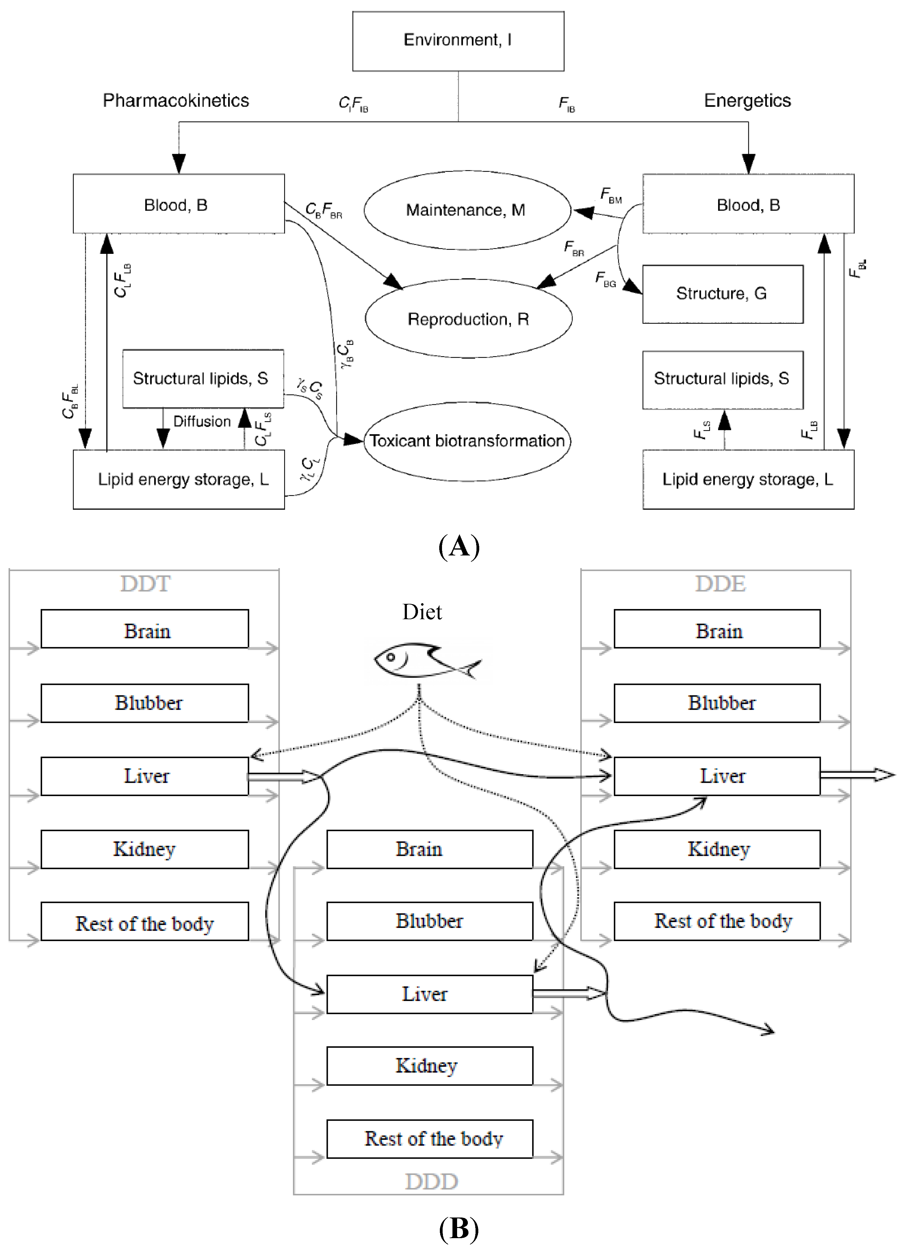
4. Bioaccumulation Models: Structure and Equations

4.1. Structure

Bioaccumulation models rely on an input and on ADME processes to generate an output. These three elements represent therefore the main structure of any bioaccumulation model. The input is the driving force that makes the bioaccumulation models run: without an input, the software is not likely going to give any output. As discussed earlier (Absorption), the most common pathway for marine mammals to absorb lipophilic chemicals is by ingestion of food (oral exposure). This automatically generates three important questions: (1) how much food does the animal require and acquire? (2) which food items are included in the diet for each species? (3) what are the concentrations of the compounds in these food items?
The first question can be interpreted from an energetic, as well as from a mass-related perspective. The animals obviously need a lot of energy for survival and reproduction and will attempt to adjust their dietary requirements accordingly. Establishing an input based on energetic requirements can be rather simple or more comprehensive. The fairly simple way can be found in Hickie et al. [12] where energy requirements were first calculated based on the animals size, growth rate, level of activity and reproductive effort (i.e., supporting gestation or lactation). This energy demand was then converted into a feeding rate, taking into account the average digestibility of the food and its energy content (e.g., fish was assumed to be composed of 15% protein with an energy content of 5650 kcal/kg). A set of similar calculations were used for nursing calves to estimate the energy and volume of milk they require which was then added to the energy requirements of the mother. One of the most sensitive and uncertain parameters in this approach has to do with the selection of the factor that accounts for the “field metabolic rate” which can be estimated as a multiplication of the estimated resting metabolic rate.
A more comprehensive (and parameter intensive) way is the one used by Klanjscek et al. [16] which focuses on the lipid dynamics. This study divided the bioaccumulation models used into two components covering both the pharmacokinetics of the (lipophilic) chemical, as well as the energetics. This is also reflected in the compartments that were included in the model: Blood, Structural lipids, Structure and Lipid energy storage (Figure 1A). None of these compartments refer to a specific organ. Compared to all marine mammal models available to date, Klanjscek et al. [16] models are unique in the sense that they follow the chemical’s “carrier” (i.e., lipids) rather than the chemical itself. Establishing an input based on mass-related requirements is a different approach that does not make any assumptions whatsoever about the energy content of food items or the energy needed by the marine mammal for survival, growth and reproduction. This specific approach requires information about how many kg of fish/milk the animals eat on a daily basis, on the diet composition and on what the concentration of the chemical of interest is in the food items included in the diet. The first factor is a body weight dependent equation that can be found in Innes et al. [46] or deduced from Kastelein [47] for a wide range of marine mammals or in several other studies for specific marine mammal species, e.g., Kastelein et al. [48] for harbour porpoises; Kastelein et al. [49] for harbour seals; Lockyer [50] for baleen fin whales, long-finned pilot whales and harbour porpoises. The second factor is the most challenging in this mass-based approach, since the diet of marine mammals changes constantly, not only for each individual, but also between seasons, years, or locations.
While bioaccumulation models for marine mammals may track the accumulation of a chemical in an individual or set of animals over time, i.e., a longitudinal view of accumulation, the datasets used for comparison typically consist of samples collected from a number of individuals from a population that ideally vary in age and gender, i.e., a cross-sectional sample of the population at the time of sampling. This would not be a problem if the diet of the sampled animals and contaminant concentrations therein did not change over time as both the model and dataset could achieve a pseudo-steady state. The effects of temporal changes in contaminant concentrations in the diet can be addressed by bioaccumulation models through careful development of long-term exposure scenarios [8]. The changes in prey selection over time or the differences in diet between individual animals pose significant challenges in both modeling efforts and interpreting contaminant datasets. Diet information may be deduced from regular feeding episodes with marine mammals in captivity, observed hunting efforts of marine mammals in the wild, stomach contents from stranded animals or from fisheries reports, among others. When stomach contents are known and concentrations of chemicals are measured, it is possible to add individual inputs for each animal in the dataset. However, since other important model parameters, e.g., metabolic biotransformation capacity, are hardly ever known on an individual level, it raises the question whether it is truly worthwhile to use individual diets in the models. The easiest way to tackle the issue of the diet composition is a food basket approach employed by Cullon et al. [51] for harbour seals (Phoca vitulina). This approach allows skipping the issue of diet composition altogether which is clearly beneficial for bioaccumulation models. Additionally, the food basket approach is a more economical way of investigating the chemical intake via food as it minimizes the number of samples that need to be analyzed.
Figure 1. Conceptual figures of the bioaccumulation models for POPs in marine mammal species. (A) is a multi-compartmental PK model for PCBs in right whales (Figure taken from Klanjscek et al. [16]). (B) is a multi-compartmental PBPK model for p,p'-DDT and its metabolites p,p'-DDD and p,p'-DDE in harbor porpoises (Figure taken from Weijs et al. [20]). In (A), C represents lipid-normalized toxicant concentration, F is energy flux, D is the diffusion coefficient between two compartments and γ is the toxicant decay (biotransformation rate). Abbreviations in subscript refer to the respective compartment(s).
Toxics 02 00226 g001
Figure 2. General schematic workflow. This scheme highlights the importance of parameter knowledge in bioaccumulation models for marine mammals as well as the “train of thoughts” on the background of model development.
Toxics 02 00226 g002
From a biological point of view, an energy-based input is perhaps the most accurate as several marine mammal species are generalist eaters: they eat whatever there is available. An energy-based input does not make any assumptions about the fish species included in the diet, although chemical concentrations in the diet are usually based on data from known or probable prey. A mass-based input on the other hand focusses usually only on a few, readily available, fish species and therefore forces the marine mammal species to be “specialist” eaters which, in essence, is not always true. From a toxicological point of view, a mass-based input is probably the most reasonable as toxicological and biomonitoring studies do not target “fish” in general, but several specific fish species with contaminant levels and profiles that reflect their lifestyle, habitat, age, reproduction status and location. All these factors are not taken into account in the energy-based input approach. There are clearly pros and cons involved for both approaches. There is no preferred or recommended approach, so the approach used in the bioaccumulation models often depends on the available dietary information for the marine mammal species of interest.
The ADME processes are situated in compartments which can be individual organs or tissues lumped together based on specific characteristics. The nomenclature of the bioaccumulation model is often derived from these compartments. If a compartment represents an anatomical entity (e.g., muscle, brain, liver) than the models are called physiologically based pharmacokinetic or toxicokinetic (PBPK or PBTK) models. If a compartment is simply a homogeneous space that not corresponds to a specific anatomical body part, than those models are classic compartmental TK models (Figure 1A,B; Table 1).

4.2. Equations

Information regarding the ADME processes can be integrated in mathematical equations and put into a broader context for example to simulate the chemical kinetics over the entire lifetime of the animals [22]. The first step in developing a bioaccumulation model is determining the level of complexity and the number of (homogenous) compartments which all depends on the questions the model has to solve and on the availability of parameter information (Figure 2). The kinetics of a chemical in the model needs to be time-dependent and able to cover a relatively large time span as some marine mammal species can grow quite old, an issue which can be solved by mass-balanced differential equations.
To ensure that the model predictions are representative for the situation in reality, the model needs to be evaluated using real life and independent datasets. If refinements are required, it is useful to know which parameters are the most important in terms of model changes. Sensitivity analyses are often performed to inform about how sensitive each parameter is with respect to the outcome of a specific endpoint in model simulation to pre-defined changes in parameter value, to assess where the sources of uncertainty are in the models and to know which parameter requires further optimization. For the latter reason, sensitivity analyses can be regarded as the connection between the structural model and the statistical supplementation (i.e., parameter estimating by statistical methods), although they are not a requirement for developing statistical supplementations. Sensitivity analyses can be “local” or “global”. During a local sensitivity analysis (LSA), the model predictions are judged against pre-defined changes of for example 1%, 2% or 5% in each separate parameter value and expressed in, for instance, area under the curve (AUC) of the model values [52]. In a global sensitivity analysis (GSA), however, all model parameters vary in pre-defined ranges and their relative influence on the model output is assessed [53]. LSA generally works fine for simple and linear models in which there are no interactions between the parameters. However, interactions between parameters are usually unavoidable in more complex models which highlights the need for methods that are more global or randomized compared to LSA [53] (Figure 2).

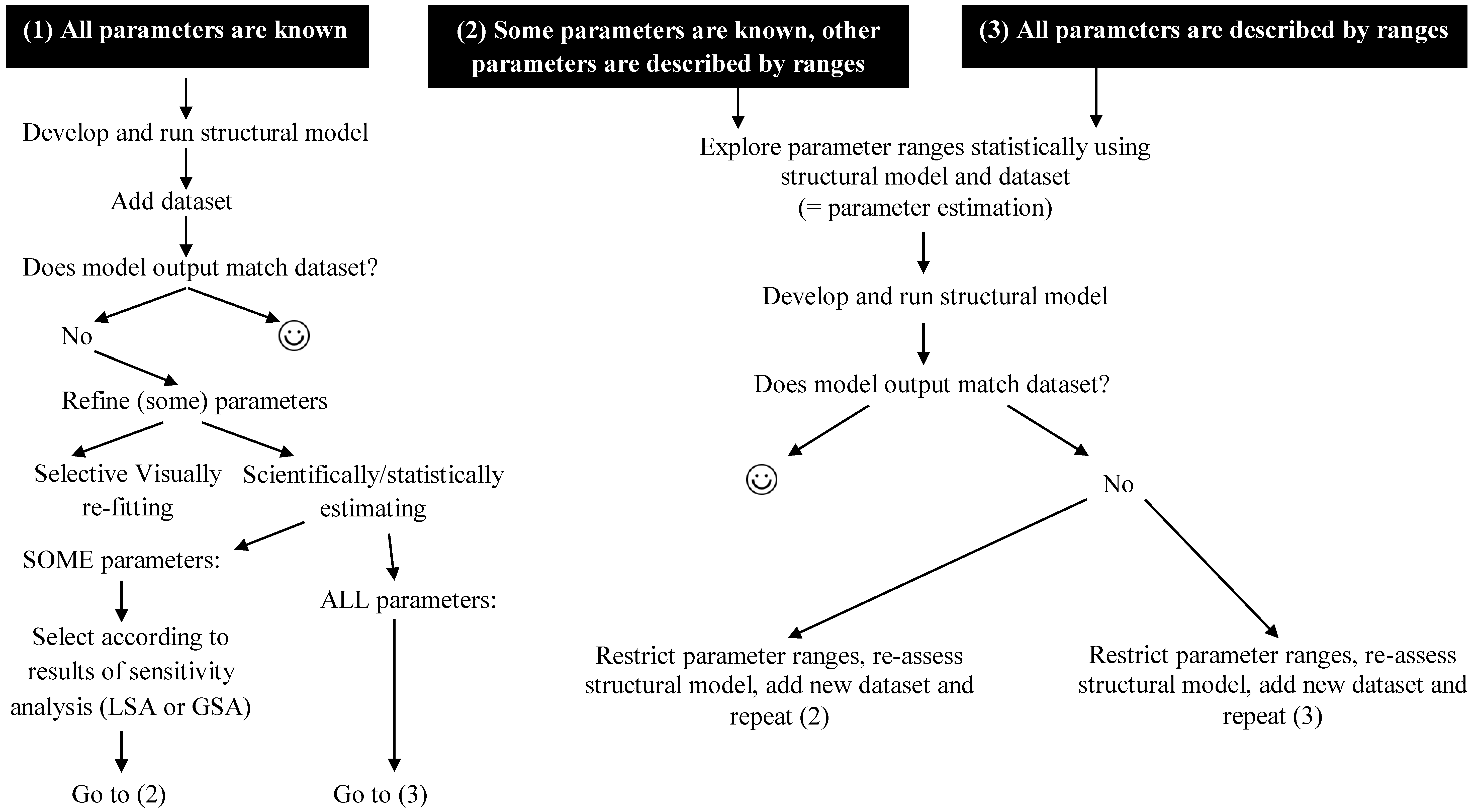
5. Bioaccumulation Models: Statistical Supplementation

The goal of a model is to show a simplified version of a usually very complex reality. Clearly, this complexity can cause some uncertainty and variability that should be addressed in a statistically sound manner [54]. Though there are several statistical methods employed for parameter estimation to minimize uncertainty and variability, the most recent and advanced one is the Bayesian approach using Markov chain Monte Carlo (MCMC) simulations (Figure 3). This approach is a way to explore the parameter probability distribution created by the variation in parameter values around a certain parameter distribution [54]. Especially in uncontrolled environments as encountered with wild animal populations, parameters tend to have ranges of potential values instead of single and fixed values. The role of the Bayesian approach with MCMC is to test all possible parameter values in the overall parameter space in order to come up with parameter values or (smaller) ranges. These posterior values or ranges are more meaningful to describe a specific dataset and by extension also the population where the dataset was taken from. The Bayesian approach allows the inclusion of prior knowledge of the parameters and is therefore totally different from any frequentist approach [55]. This prior knowledge can relate to specific parameter values or parameter ranges taken from the literature, even from other species, or updated results of previous model runs. Bayes’ theorem is based on:
p(θ|d) ∝ p(θ) · p(d|θ)
where d stands for the data, θ for the parameter values, p(θ|d) for the posterior distribution of the parameters given the data, p(θ) for the prior distribution of the parameters and p(d|θ) the likelihood of the data given the parameters [55]. If the prior distribution of the parameters is uninformative, this method will give the same parameter means as the maximum likelihood estimation (MLE) which is a frequentist approach as used in the bioaccumulation model for bottlenose dolphins [7].
Monte Carlo is an efficient numerical way to repeatedly draw samples from a (prior) distribution in order to estimate averages and variances, thus posterior parameter distributions. Combined with Bayes’ theorem, this prior distribution is formed by the likelihood of the data given the parameters and the prior knowledge of the data. Markov chains are applied to optimize the ‘repeatedly drawing samples’ part inasmuch that every drawing depends on the immediately preceding one thereby creating chains. The impact of Markov chains on the Monte Carlo method is thus that the posterior parameter distribution is going to be different and narrower if the prior parameter knowledge is sufficiently informative (Figure 3).
The Bayes’ theorem combined with MCMC simulations approach can be applied for multiple datasets. Prior values of parameters from the literature (even from other species) and dataset A can yield posterior distributions of the initial, prior parameter values. These posterior distributions can be used as prior parameter distributions in the next successive parameter estimation approach using dataset B. Repeating this process for datasets C, D and E will finally result in parameter estimates that are suitable for datasets A–E. Assuming that datasets are different populations from the same animal species as in this work, the parameter estimates will be representative for the entire population. This Bayesian approach with MCMC simulations has been used so far in bioaccumulation models for harbor porpoises and long-finned pilot whales (AcslX/Libero software and MCSim; [20,21]).
Figure 3. Illustration showing the difference between MCMC sampling ( Toxics 02 00226 i001) and simple Monte Carlo sampling ( Toxics 02 00226 i002
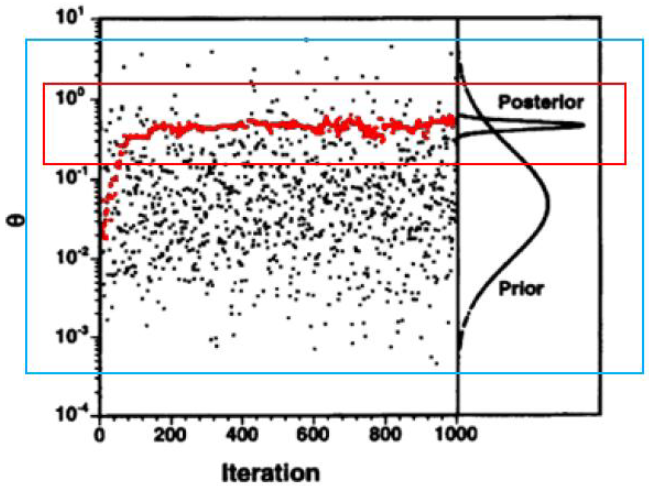
). Y-axis represents the parameter values (θ), X-axis represents the number of iterations (parameter drawings or model runs). Figure adjusted from Bernillon and Bois [53].
Toxics 02 00226 g003

6. Concluding Remarks and Future Directions

Bioaccumulation models are a representation or estimation of reality. “Reality” for marine mammals, however, is largely unknown, scattered or, at best, relatively well-documented for specific populations. Despite all possible statistical tests or analyses, the accuracy of exposure models for marine mammals depends on having sufficient information for model development. Modeling is therefore not a stand-alone process, but benefits greatly from all information made available by other scientists in the field. “Reality” changes continuously, so models change as well. This is not only the reason why there are several model types for marine mammals available, but it also explains why current models should change continuously. The bioaccumulation models developed so far are fairly new in the field of marine mammal toxicology. These models can and should be expanded in the future in order to facilitate our understanding of the health situation of marine mammals in the past, present and future. In this regard, the word “expand” refers to:

6.1. Adding more Datasets

Most bioaccumulation models for marine mammals to date are mainly developed for one specific dataset or population. Statistical techniques, such as the Bayesian approach and MCMC simulations, allow the addition of multiple datasets, thereby creating smaller parameter ranges and state-of-the-art parameter values that are effective for multiple datasets or populations. Bioaccumulation models in which the parameter values are attached to a single dataset, are basically only population-specific. Bioaccumulation models in which the parameter values are attached to a series of datasets, are suitable for several populations and may be broadly applied for that species. For risk assessment purposes, such robust species-specific models are more attractive than population-specific models as scenarios from the past, present and future can be judged for much larger groups of animals and may be applied with some confidence for populations where data are limited.

6.2. Adding more Compartments

Models should reflect the reality as well as possible, e.g., marine mammals are composed of multiple compartments/tissues. An organism is a complex system in which each cell or tissue has a function and perhaps an impact on the kinetics and distribution of a chemical inside the body. Of course, depending on the chemical and on the availability of information about the tissues in a specific species, simple, even one-compartment models can suit the purpose. Yet, to fully understand the kinetics of a chemical and its effect on an organism, one-compartment models are not helpful as they actually only give the deposition of a chemical in that compartment instead of its kinetics in the body. Adding more compartments should be done judiciously with heed to the old adage that a model should be “as simple as possible and as complex as necessary”.

6.3. Coupling to an Effects or Dynamic Model

Effects can be visible on multiple levels and are usually visible through a cascade of molecular changes. If it would be possible to translate that cascade of changes into mathematical equations and add it to bioaccumulation models, there would be models that explain the kinetics of a chemical as well as its effect on the animal at the same time. Such a combination of a kinetic and dynamic model would give a more thorough overview of the marine mammal’s exposure to a certain chemical than any existing bioaccumulation model to date and would be highly desired for risk assessment purposes. Combinations of bioaccumulation models and effect studies are already available for killer whales and harbor porpoises [8,56]. Though these combinations are technically not pharmacokinetic/pharmacodynamics models, they show that combinations of bioaccumulation models and effects can be used for predictions in the future. According to Hickie et al. [8], levels of PCBs in the southern resident killer whales will largely fall below health effects thresholds established for marine mammals around 2063. According to Weijs [56], levels of PCB 153 in harbor porpoises of the North Sea will be below effect levels reported for harbour porpoises by Das et al. [57] in 2051.

6.4. Extrapolating to Other Species/Chemicals

Though there are already a substantial number of models available for several types of chemicals in various marine mammal species, it would be desirable to develop models that could be applied to other marine mammal species and classes of chemicals. While it would be ideal to develop separate models for each species that could be applied to multiple classes of chemicals, this is not practical given the great number of marine mammal species and wide variation in chemical characteristics. Therefore, it would be worthwhile to investigate whether and how models could be developed for groups of species with similar life history traits that would require little effort to adapt to other species in the group or how models for the bioaccumulation of, for example, PCB 153 could be used for explaining the bioaccumulation of PBDE 153 in a specific species.
By expanding the current bioaccumulation models in all possible directions, they can be used and explored to the maximum of their potential. Bioaccumulation models are not limited in space or time as they can provide information about past, current and potential future exposure scenarios in marine mammal species worldwide. A tool that integrates knowledge from different fields of research and that can anticipate the potential impact of new chemicals can only be beneficial for risk assessment and conservation of marine mammal species.

Acknowledgments

LW acknowledges financial support from the FWO (Fonds Wetenschappelijk Onderzoek-Vlaanderen; Scientific Research Funds-Flanders) and University of Antwerp.

Conflicts of Interest

The authors declare no conflict of interest.

References

  1. Timchalk, C.; Nolan, R.J.; Mendrala, A.L.; Dittenber, D.A.; Brzak, K.A.; Mattson, J.L. A physiologically based pharmacokinetic and pharmacodynamics (PBPK/PD) model for the organophosphate insecticide chlorpyrifos in rats and humans. Toxicol. Sci. 2002, 66, 34–53. [Google Scholar] [CrossRef]
  2. Ling, M.P.; Liao, C.M. A human PBPK/PD model to assess arsenic exposure risk through farmed tilapia consumption. Bull. Environ. Contam. Toxicol. 2009, 83, 108–114. [Google Scholar] [CrossRef]
  3. Liao, C.M.; Liang, H.M.; Chen, B.C.; Singh, S.; Tsai, J.W.; Chou, Y.H.; Lin, W.T. Dynamical coupling of PBPK/PD and AUC-based toxicity models for arsenic in tilapia Oreochromis mossambicus from blackfoot disease area in Taiwan. Environ. Pollut. 2005, 135, 221–233. [Google Scholar] [CrossRef]
  4. Abbas, R.; Hayton, W.L. A physiologically based pharmacokinetic and pharmacodynamics model for paraoxon in rainbow trout. Toxicol. Appl. Pharmacol. 1997, 145, 192–201. [Google Scholar] [CrossRef]
  5. Clewell, H.J., III; Andersen, M.E. Use of physiologically based pharmacokinetic modeling to investigate individual versus population risk. Toxicology 1996, 111, 315–329. [Google Scholar] [CrossRef]
  6. Lipscomb, J.C.; Haddad, S.; Poet, T.; Krishnan, K. Physiologically-Based Pharmacokinetic (PBPK) Models in Toxicity Testing and Risk Assessment. In New Technologies for Toxicity Testing; Balls, M., Combes, R.D., Bhogal, N., Eds.; Springer US: New York, NY, USA, 2012; pp. 76–95. [Google Scholar]
  7. Hall, A.J.; McConnell, B.J.; Rowles, T.K.; Aguilar, A.; Borrell, A.; Schwacke, L.; Reijnders, P.J.; Wells, R.S. Individual-based model framework to assess population consequences of polychlorinated biphenyl exposure in bottlenose dolphins. Environ. Health Perspect. 2006, 114, 60–64. [Google Scholar]
  8. Hickie, B.E.; Ross, P.S.; MacDonald, R.W.; Ford, J.K.B. Killer whales (Orcinus orca) face protracted health risks associated with lifetime exposure to PCBs. Environ. Sci. Technol. 2007, 41, 6613–6619. [Google Scholar] [CrossRef]
  9. Hickie, B.E.; Cadieux, M.A.; Riehl, K.N.; Bossart, G.D.; Alava, J.J.; Fair, P.A. Modeling PCB-bioaccumulation in the bottlenose dolphin (Tursiops truncatus): Estimating a dietary threshold concentration. Environ. Sci. Technol. 2013, 47, 12314–12324. [Google Scholar] [CrossRef]
  10. Bouzom, F.; Ball, K.; Perdaems, N.; Walther, B. Physiologically based pharmacokinetic (PBPK) modeling tools: How to fit with our needs? Biopharm. Drug Dispos. 2012, 33, 55–71. [Google Scholar] [CrossRef]
  11. Schmitt, W.; Willmann, S. Physiologically-based pharmacokinetic modeling: Ready to be used. Drug Discov. Today 2005, 2, 125–132. [Google Scholar] [CrossRef]
  12. Hickie, B.E.; Mackay, D.; de Koning, J. Lifetime pharmacokinetic model for hydrophobic contaminants in marine mammals. Environ. Toxicol. Chem. 1999, 18, 2622–2633. [Google Scholar] [CrossRef]
  13. Hickie, B.E.; Kingsley, M.C.S.; Hodson, P.V.; Muir, D.C.G.; Béland, P.; Mackay, D. A modeling-based perspective on the past, present, and future polychlorinated biphenyl contamination of the St. Lawrence beluga whale (Delphinapterus leucas ) population. Can. J. Fish. Aquat. Sci. 2000, 57, 101–112. [Google Scholar] [CrossRef]
  14. Hickie, B.E.; Muir, D.C.G.; Addison, R.F.; Hoekstra, P.F. Development and application of bioaccumulation models to assess persistent organic pollutant temporal trends in arctic ringed seal (Phoca vitulina) populations. Sci. Total Environ. 2005, 351–352, 413–426. [Google Scholar]
  15. Mongillo, T.M.; Holmes, E.E.; Noren, D.P.; VanBlaricom, G.R.; Punt, A.E.; O’Neill, S.M.; Ylitalo, G.; Hanson, M.B.; Ross, P.S. Predicted polybrominated diphenyl ether (PBDE) and polychlorinated biphenyl (PCB) accumulation in southern resident killer whales. Mar. Ecol. Prog. Ser. 2012, 453, 263–277. [Google Scholar] [CrossRef]
  16. Klanjscek, T.; Nisbet, R.M.; Caswell, H.; Neubert, M.G. A model for energetics and bioaccumulation in marine mammals with applications to the right whale. Ecol. Appl. 2007, 17, 2233–2250. [Google Scholar] [CrossRef]
  17. Weijs, L.; Yang, R.S.H.; Covaci, A.; Das, K.; Blust, R. Physiologically based pharmacokinetic models for lifetime exposure to PCB 153 in male and female harbour porpoises (Phocoena phocoena): Model development and validation. Environ. Sci. Technol. 2010, 44, 7023–7030. [Google Scholar] [CrossRef]
  18. Weijs, L.; Covaci, A.; Yang, R.S.H.; Das, K.; Blust, R. A non-invasive approach to study lifetime exposure and bioaccumulation of PCBs in protected marine mammals: PBPK modeling in harbour porpoises. Toxicol. Appl. Pharmacol. 2011, 256, 136–145. [Google Scholar] [CrossRef]
  19. Weijs, L.; Covaci, A.; Yang, R.S.H.; Das, K.; Blust, R. Computational toxicology: Physiologically based pharmacokinetic models (PBPK) for lifetime exposure and bioaccumulation of polybrominated diphenyl ethers (PBDEs) in marine mammals. Environ. Pollut. 2012, 163, 134–141. [Google Scholar] [CrossRef]
  20. Weijs, L.; Yang, R.S.H.; Das, K.; Blust, R.; Covaci, A. Application of Bayesian population PBPK modeling and Markov chain Monte Carlo simulations to pesticide kinetics studies in protected marine mammals: DDT, DDE, DDD in harbour porpoises. Environ. Sci. Technol. 2013, 47, 4365–4374. [Google Scholar] [CrossRef]
  21. Weijs, L.; Roach, A.C.; Yang, R.S.H.; McDougall, R.; Lyons, M.; Housand, C.; Tibax, D.; Manning, T.M.; Chapman, J.C.; Edge, K.; et al. Lifetime PCB 153 bioaccumulation and pharmacokinetics in pilot whales: Bayesian population PBPK modeling and Markov chain Monte Carlo simulations. Chemosphere 2014, 94, 91–96. [Google Scholar] [CrossRef]
  22. Gobas, F.; Arnot, J. 2005 San Francisco Bay PCB Food Web Bioaccumulation Model. Final Technical Report. Available online: http://www.bacwa.org/Portals/0/Committees/Clean%20Estuary%20Partnership/Library/Task4.27-FoodWebModel.pdf (accessed on 5 June 2008).
  23. CRC. Handbook of Marine Mammal Medicine, 2nd ed.; Dierauf, L.A., Gulland, F.M.D., Eds.; CRC Press LCC: Boca Raton, FL, USA, 2001; p. 1120. [Google Scholar]
  24. Encyclopedia of Marine Mammals, 2nd ed.; William, P.; Bernd, W.; Thewissen, J. (Eds.) Academic Press: Sandiago, CA, USA, 2008; p. 1352.
  25. Oftedal, O.T. Lactation in whales and dolphins: Evidence of divergence between baleen- and toothed species. J. Mammary Gland Biol. Neoplasia 1997, 2, 205–230. [Google Scholar] [CrossRef]
  26. Brown, R.P.; Delp, M.D.; Lindstedt, S.L.; Rhomberg, L.R.; Beliles, R.P. Physiological parameter values for physiologically based pharmacokinetic models. Toxicol. Ind. Health 1997, 13, 407–484. [Google Scholar] [CrossRef]
  27. Noonburg, E.G.; Nisbet, R.M.; Klanjscek, T. Effects of life history variation on vertical transfer of toxicants in marine mammals. J. Theor. Biol. 2010, 264, 479–489. [Google Scholar] [CrossRef]
  28. Clewell, R.A.; Clewell, H.J., III. Development and specification of physiologically based pharmacokinetic models for use in risk assessment. Regul. Toxicol. Pharmacol. 2008, 50, 129–143. [Google Scholar] [CrossRef]
  29. Duarte-Davidson, R.; Jones, K.C. Polychlorinated biphenyls (PCBs) in the UK population: Estimated intake, exposure and body burden. Sci. Total Environ. 1994, 151, 131–152. [Google Scholar] [CrossRef]
  30. Hui, C. Seawater consumption and water flux in the common dolphin Delphinus delphis. Physiol. Zool. 1981, 54, 430–440. [Google Scholar]
  31. Ortiz, R. Osmoregulation in marine mammals. J. Exp. Biol. 2001, 204, 1831–1844. [Google Scholar]
  32. Thomas, G.O.; Moss, S.E.W.; Asplund, L.; Hall, A.J. Absorption of decabromodiphenyl ether and other organohalogen chemicals by grey seals (Halichoerus grypus). Environ. Pollut. 2005, 133, 581–586. [Google Scholar] [CrossRef] [Green Version]
  33. Parham, F.M.; Kohn, M.C.; Matthews, H.B.; DeRosa, C.; Portier, C.J. Using structural information to create physiologically based pharmacokinetic models for all polychlorinated biphenyls. I. Tissue:blood partition coefficients. Toxicol. Appl. Pharmacol. 1997, 144, 340–347. [Google Scholar] [CrossRef]
  34. Thornton, S.J.; Hochachka, P.W.; Crocker, D.E.; Costa, D.P.; LeBoeuf, B.J.; Spielman, D.M.; Pelc, N.J. Stroke volume and cardiac output in juvenile elephant seals during forced dives. J. Exp. Biol. 2005, 208, 3637–3643. [Google Scholar] [CrossRef]
  35. Svendsgaard, D.J.; Ward, T.R.; Tilson, H.A.; Kodavanti, P.R.S. Emperical modeling of an in vitro activity of polychlorinated biphenyl congeners and mixtures. Environ. Health Perspect. 1997, 105, 1106–1115. [Google Scholar] [CrossRef]
  36. Braekevelt, E.; Tittlemier, S.A.; Tomy, G.T. Direct measurement of octanol-water partition coefficients of some environmentally relevant brominated diphenyl ether congeners. Chemosphere 2003, 51, 563–567. [Google Scholar] [CrossRef]
  37. Hayward, S.J.; Lei, Y.D.; Wania, F. Comparative evaluation of three high-performance liquid Chromatography-based Kow estimation methods for highly hydrophobic organic compounds: Polybrominated diphenyl ethers and hexabromocyclododecane. Environ. Toxicol. Chem. 2006, 25, 2018–2027. [Google Scholar] [CrossRef]
  38. Letcher, R.J.; Klasson-Wehler, E.; Bergman, A. Methyl Sulfone and Hydroxylated Metabolites of Polychlorinated Biphenyls. In The Handbook of Environmental Chemistry; Paasivirta, J., Ed.; Part K, New Types of Persistent Halogenated Compounds; Springer-Verlag: Heidelberg/Berlin, Germany, 2000; Volume 3. [Google Scholar]
  39. Redding, L.E.; Sohn, M.D.; McKone, T.E.; Chen, J.W.; Wang, S.L.; Hsieh, D.P.H.; Yang, R.S.H. Population physiologically based pharmacokinetic modeling for the human lactational transfer of PCB 153 with consideration of worldwide human biomonitoring results. Environ. Health Perspect. 2008, 116, 1629–1634. [Google Scholar] [CrossRef]
  40. Verner, M.A.; Charbonneau, M.; Lopez-Carrillo, L.; Haddad, S. Physiologically based pharmacokinetic modeling of persistent organic pollutants for lifetime exposure assessment: A new tool in breast cancer epidemiologic studies. Environ. Health Perspect. 2008, 116, 886–892. [Google Scholar] [CrossRef]
  41. Miniero, R.; de Felip, E.; Ferri, F.; di Domenico, A. An overview of TCDD half life in mammals and its correlation to body weight. Chemosphere 2001, 43, 839–844. [Google Scholar] [CrossRef]
  42. Agency for Toxic Substances and Disease Registry (ATSDR). 2001; Polychlorinated biphenyls. US Department of Health and Human Services. Available online: http://www.atsdr.cdc.gov/toxfaqs/index.asp (accessed 5 June 2008). [Google Scholar]
  43. Staskal, D.F.; Diliberto, J.J.; DeVito, M.J.; Birnbaum, L.S. Toxicokinetics of BDE 47 in female mice: Effect of dose, rout of exposure, and time. Toxicol. Sci. 2005, 83, 215–223. [Google Scholar]
  44. Li, H.X.; Boon, J.P.; Lewis, W.E.; van den Berg, M.; Nyman, M.; Letcher, R.J. Hepatic microsomal cytochrome P450 enzyme activity in relation to in vitro metabolism/inhibition of polychlorinated biphenyls and testosterone in Baltic grey seal (Halichoerus grypus). Environ. Toxicol. Chem. 2003, 22, 636–644. [Google Scholar] [CrossRef]
  45. McKinney, M.A.; de Guise, S.; Martineau, D.; Béland, P.; Arukwe, A.; Letcher, R.J. Biotransformation of polybrominated diphenyl ethers and polychlorinated biphenyls in beluga whale (Delphinapterus leucas) and rat mammalian model using an in vitro hepatic microsomal assay. Aquat. Toxicol. 2006, 77, 87–97. [Google Scholar] [CrossRef]
  46. Innes, S.; Lavigne, D.M.; Earle, W.M.; Kovacs, K.M. Feeding rates of seals and whales. J. Anim. Ecol. 1987, 56, 115–130. [Google Scholar] [CrossRef]
  47. Kastelein, R.A. Food Consumption and Growth of Marine Mammals. Ph.D. Dissertation, Landbouwuniversiteit, Wageningen, The Netherlands, 1998; p. 647. [Google Scholar]
  48. Kastelein, R.A.; Hardeman, J.; Boer, H. Food Consumption and Body Weight of Harbour Porpoises (Phocoena phocoena). In The Biology of the Harbour Porpoise; Read, A.J., Wiepkema, P.R., Nachtigall, P.E., Eds.; De Spil Publishers: Woerden, The Netherlands, 1997; pp. 217–233. [Google Scholar]
  49. Kastelein, R.A.; Staal, C.; Wiepkema, P.R. Food consumption and body mass of captive harbour seals Phoca vitulina. Aquat. Mamm. 2005, 31, 34–42. [Google Scholar] [CrossRef]
  50. Lockyer, C. All creatures great and smaller: A study in cetacean life history energetics. J. Mar. Biol. Assoc. UK 2007, 87, 1035–1045. [Google Scholar] [CrossRef]
  51. Cullon, D.L.; Jeffries, S.J.; Ross, P.S. Persistent organic pollutants in the diet of harbour seals (Phoca vitulina) inhabiting Puget Sound, Washington (USA), and the Strait of Georgia, British Columbia (Canada): A food basket approach. Environ. Toxicol. Chem. 2005, 24, 2562–2572. [Google Scholar] [CrossRef]
  52. Emond, C.; Raymer, J.H.; Studabaker, W.B.; Garner, C.E.; Birnbaum, L.S. A physiologically based pharmacokinetic model for developmental exposure to BDE-47 in rats. Toxicol. Appl. Pharmacol. 2010, 242, 290–298. [Google Scholar] [CrossRef]
  53. McNally, K.; Cotton, R.; Loizou, G.D. A workflow for global sensitivity analysis of PBPK models. Front. Pharmacol. 2011, 2, 1–21. [Google Scholar]
  54. Bernillon, P.; Bois, F.Y. Statistical issues in toxicokinetic modeling: A Bayesian perspective. Environ. Health Perspect. 2000, 108, 883–893. [Google Scholar] [CrossRef]
  55. Hack, C.E. Bayesian analysis of physiologically based toxicokinetic and toxicodynamic models. Toxicology 2006, 221, 241–248. [Google Scholar] [CrossRef]
  56. Weijs, L. Development of Physiologically Based Pharmacokinetic Models for the Bioaccumulation of Persistent Organic Pollutants in Marine Mammals. Ph.D. Dissertation, University of Antwerp, Antwerpen, Belgium, May 2013. [Google Scholar]
  57. Das, K.; Vossen, A.; Tolley, K.; Vikingsson, G.; Thron, K.; Baumgärtner, W.; Siebert, U. Interfollicular fibrosis in the thyroid of the harbour porpoise: An endocrine disruption? Arch. Environ. Contam. Toxicol. 2006, 52, 720–729. [Google Scholar]

