Hydrodynamics of Bubble Columns: Turbulence and Population Balance Model


Chemical Engineering Department, Université de Sherbrooke, Sherbrooke, QC, J1K 2R1, Canada
*
Author to whom correspondence should be addressed.
†
Current address: Research Center in Aerospace Engineering, Cenaero, 6041 Gosselies, Belgium.
ChemEngineering 2018, 2(1), 12; https://doi.org/10.3390/chemengineering2010012
Submission received: 13 February 2018
/
Revised: 10 March 2018
/
Accepted: 12 March 2018
/
Published: 19 March 2018
(This article belongs to the Special Issue Bubble Column Fluid Dynamics)
Abstract
:This paper presents an in-depth numerical analysis on the hydrodynamics of a bubble column. As in previous works on the subject, the focus here is on three important parameters characterizing the flow: interfacial forces, turbulence and inlet superficial Gas Velocity (UG). The bubble size distribution is taken into account by the use of the Quadrature Method of Moments (QMOM) model in a two-phase Euler-Euler approach using the open-source Computational Fluid Dynamics (CFD) code OpenFOAM (Open Field Operation and Manipulation). The interfacial forces accounted for in all the simulations presented here are drag, lift and virtual mass. For the turbulence analysis in the water phase, three versions of the Reynolds Averaged Navier-Stokes (RANS) k-ε turbulence model are examined: namely, the standard, modified and mixture variants. The lift force proves to be of major importance for a trustworthy prediction of the gas volume fraction profiles for all the (superficial) gas velocities tested. Concerning the turbulence, the mixture k-ε model is seen to provide higher values of the turbulent kinetic energy dissipation rate in comparison to the other models, and this clearly affects the prediction of the gas volume fraction in the bulk region, and the bubble-size distribution. In general, the modified k-ε model proves to be a good compromise between modeling simplicity and accuracy in the study of bubble columns of the kind undertaken here.
1. Introduction
Two-phase flow is a major topic of study in diverse research projects, due simply to the fact that it is a phenomenon occurring in many industrial flow situations, and because a rich body of information has been accrued to support advanced fluid dynamic studies of the subject for model validation.
Bubble columns in particular are widely used as test cases for experimental analysis of dispersed two-phase flows [1,2,3], since they entail simple geometric configurations, and are able to provide useful data for the validation of the CFD models [4]. Table 1 provides a comprehensive list of some of the most referenced experimental studies in this area.
Both the global and local properties of the flow in bubble columns are related to the existing flow regime, which can be defined as homogeneous or heterogeneous, depending on the prevailing bubble size [5]. If the bubbles are in the range of 0.001–0.007 m and the superficial gas velocity is less than 0.05 m/s, the flow can be defined as homogeneous [5,6,7].
According to Besagni et al. [8], homogeneous flow (as that studied in the present work) is characterized by the gas phase being uniformly distributed in the liquid phase as discrete bubbles [9]. This characterization can be further designated mono-dispersed flow or poly-dispersed flow (also known as “pseudo-homogeneous flow”). Mono-dispersed flow, as the name implies, is characterized by a single bubble-size distribution and a flat local void fraction, while poly-dispersed flow involves bubbles of different sizes and a local void fraction profile with a central peak [5,8].
Most of the cited experimental papers provide local flow data (i.e., velocities and gas volume fractions) for different superficial inlet gas velocities (in homogeneous and heterogeneous ranges), but only a few provide data on the turbulence characteristics [10,11]. This is unfortunate, since turbulence in the liquid phase is known to play an important role in the local gas distribution in the numerical simulation of dispersed bubbles [10].
Many numerical works have studied the effects of different turbulence models in bubble columns for constant-diameter bubbles (as seen in Table 2). As reported by Liu and Hinrichsen [12], this assumption is justified for bubble columns with low inlet gas velocity (up to 0.04 m/s), and for low void fraction. However, more advanced models are required to predict other phenomena occurring in the flow, such as coalescence and breakup of the bubbles, induced by the turbulent eddies, especially in flows where mass transfer (i.e., boiling) plays an important role independently of the inlet gas velocity [13]. Consequently, bubble size distribution has normally been coupled with CFD by means of models capable of solving for the population balance.
Population balance is a continuity condition written on terms of the Number Density Function (NDF), which itself is a variable containing information on how the population of the dispersed phase, particles or bubbles, inside an infinitesimal control volume is distributed over the properties of interest (volume, velocity or length, for instance) of the continuous phase. NDF is defined in terms of an internal coordinate of the elements of the dispersed phase, i.e., particle/bubble size, volume or velocity, and in terms of the external coordinates, i.e., physical position and time [14].
The population balance equation, as defined by Ramkrishna [15], is a partial integro-differential equation that defines the evolution of the NDF (see Section 3.1). In the present work the length-based NDF, , is considered, since our primary interest is in the evolution of the diameter of a bubble.
Different methods exist for numerically solving the population balance equation [13,14], such as the class method [16], Monte Carlo [17], the Method of Moments (MOM) [18], as well as the Quadrature Method of Moments (QMOM) and Direct QMOM (DQMOM) [19]. The QMOM approach was first proposed by McGrow [18] for aerosol distributions, but it has also been shown to be suitable for modelling different dispersed flow regimes involving aggregation and coagulation issues [14].
QMOM, in contrast to the class method, solves the population balance equation by considering the concept of moments, which are obtained after integration of the NDF transport equation along the particle/bubble length, using a quadrature approximation to estimate this integral (see Section 3.1). Normally, just three quadrature nodes giving six moments, are sufficient to provide a reliable bubble distribution. This method is then generally less expensive in terms of CPU time than the discrete method [13].
In several industrial applications of bubble reactors, especially for those in which mass transfer and chemical reactions occur, bubble coalescence and break-up lead to the formation of thin films, fine drops and threads of much smaller scale than that of the average bubble [20,21]. Interactions taking place at these smaller scales could eventually result in a larger range of scales needing to be considered, and treated differently. Aboulhasanzadeh et al. [20] have developed a multi-scale model that allows mass diffusion to be incorporated into Direct Numerical Simulation (DNS) of bubbly flows and predict in more detail the mass transfer between moving bubbles. This multi-scale approach, together with population balance models, can provide very deep understanding of the various phenomena occurring in multi-phase flows [20,21].
In the present work, Euler-Euler simulations are carried out for turbulent “pseudo-homogeneous” two-phase flows in a scaled-up bubble column similar to the experimental test case of Pfleger et al. [22], but with the bubble size distribution determined using QMOM. Three different superficial gas velocities, 0.0013, 0.0073 and 0.02 m/s are studied, for which bubble coalescence rather than bubble breakup is the predominant bubble interaction mechanism for the dispersed phase. It is important to mention here that the use of a population balance model for the considered inlet velocities is merely to provide a deeper understanding of the possible phenomena occurring in the dispersed flow, and not to provide any comparison with constant bubble diameter results, which has already been done by Bannari et al. [23], and Gupta and Roy [13], for instance.
Three different variants of the k- turbulence model are used to predict the liquid flow patterns inside the bubble column. The choice of Reynolds Averaged Navier-Stokes (RANS) models is based on the fact that they represent a simple implementation of the turbulence effects, with much lower computational effort, compared to Large Eddy Simulation (LES) and the anisotropic Reynolds Stress Model (RSM), for example, and that they are already widely used for two-phase flow simulations [24].
The main contribution of this work lies in the attempt to better understand the flow by specific investigation of the bubble diameter distribution, the gas-holdup, the axial liquid velocity, as well as the turbulent dissipation rate, which represents the coupling between the turbulence and the bubble-size distribution. This work is motivated by the need for better understanding of the hydrodynamics of gas-liquid flow in the design of bubble reactors, particularly for those who are unfamiliar with the topic of two-phase flow modeling. Very careful selection of the experimental data suitable for the validation of the models is presented, and the underlying physics explained in detail. The ultimate goal is to provide an overview of the main parameters affecting the flow patterns of the bubbles in water columns, and, through comparison with experimental data, to provide recommending options for solving similar problems.
2. Physical Model
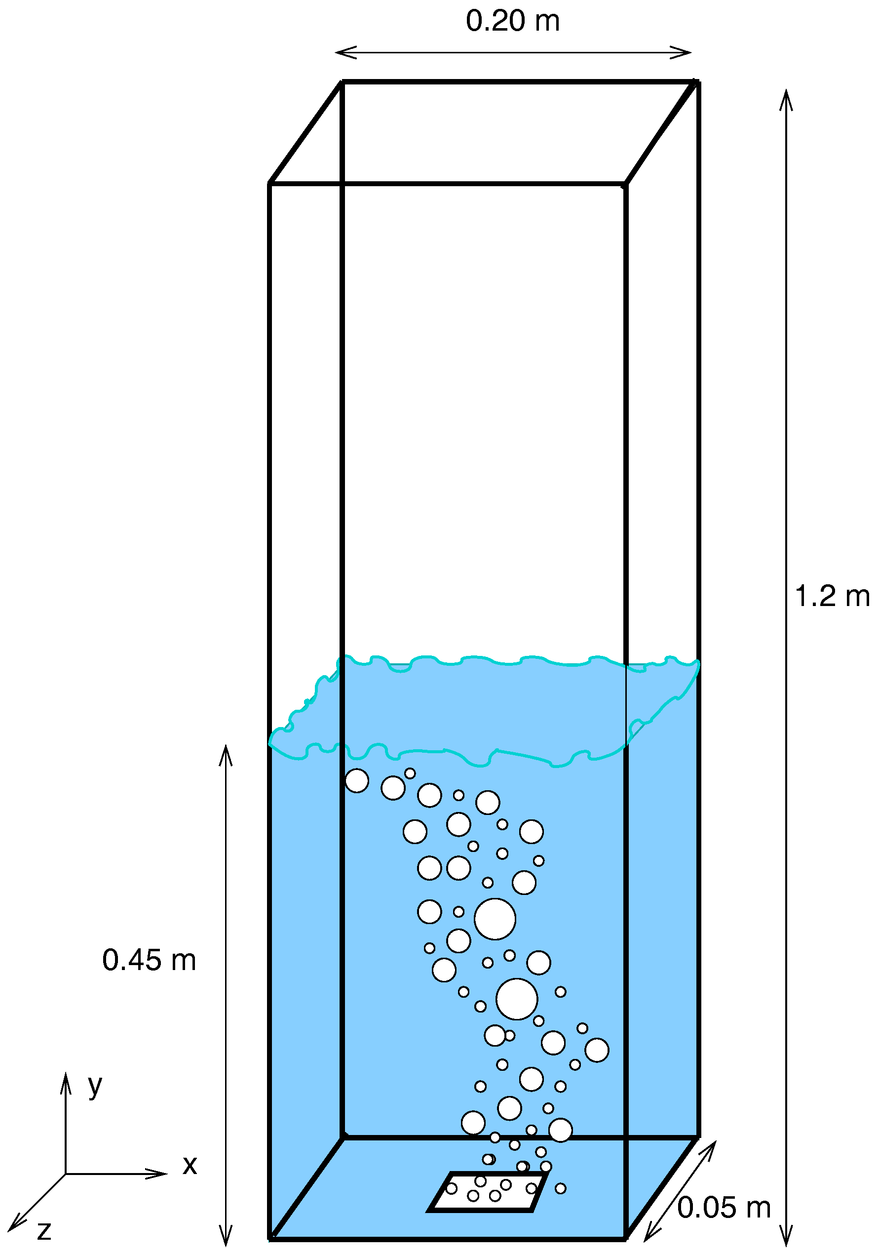
All the numerical simulations presented here are performed for a scaled-up rectangular bubble column geometry. This configuration is chosen because comprehensive experimental data exists concerning gas hold-up and liquid velocity; those provided by Pfleger et al. [22], Buwa et al. [35] and Upadhyay et al. [11] in particular are used here for model validation purposes. As depicted in Figure 1, the column is of width (W) 0.20 m, height (H) 1.2 m and depth 0.05 m. The level of water corresponds to = 2.25, a value inspired by all the tests performed by the preceding work of Becker et al. [29]. The bubbles are introduced via a sparger at the bottom.
In the experimental facility of Pfleger et al. [22], the sparger consists of a set of 8 holes placed in a rectangular configuration for the gas injection, each hole having a diameter of 0.0008 m in a square pitch of 0.006 m [13]. For simplicity, the sparger in our numerical simulations is represented by a simple rectangular area placed at the bottom of the column. The same simplification has been used in other numerical works based on this test [13,39].
3. Governing Equations
The governing equations of mass continuity and momentum for two-phase flow with no heat transfer, following the two-fluid methodology (e.g., Versteeg and Malalasekera [44]), can be expressed as follows:
where i denotes the fluid phase (liquid or gas), the phase velocity vector, the phase fraction, p the pressure, the turbulent Reynolds stress and the interfacial momentum transfer between the phases, which in this work are comprised of the drag (), lift () and virtual mass () forces. This choice follows previous studies on this topic, which showed that these three forces are enough to capture the bubble behavior in the velocity range studied here [13,37]. The turbulent dispersion force has been neglected, since previous studies have already found that, for the range of superficial gas velocities considered in this work, its influence is insignificant [45,46].
The drag force, also known as the resistance experienced by a body moving in the liquid [24], ultimately determines the gas phase residence time and thereby the bubble velocities, and greatly influences the macroscopic flow patterns [47]. It is defined as follows:
The subscripts G and L in the above equation denote gas and liquid phases respectively, and the Sauter mean diameter (explained in Section 3.1). The drag coefficient is modelled according to Schiller and Naumann [48],
where is the relative Reynolds number defined as
The lift force, which arises from the interaction between the dispersed phase and shear stress in the continuous phase, is directed perpendicular to the incoming flow, and is described as:
One of the lift coefficients used here is from Tomiyama et al. [49] (see Equation (7)), which has also been used by Gupta and Roy [13], Liu and Hinrichsen [12], and Ekambara and Dhotre [24]. For comparison purposes, constant values ( 0.14 and 0.5) have also been examined.
in which,
and given by the Wellek et al. [50] correlation:
where is the surface tension between air and water (0.07 N/m).
Finally, the virtual mass force , which refers to the inertia added to the dispersed phase due to its acceleration with respect to the heavier continuous phase, is defined as
Here the coefficient is taken to be 0.5, based on the experimental study of Odar and Hamilton [51].
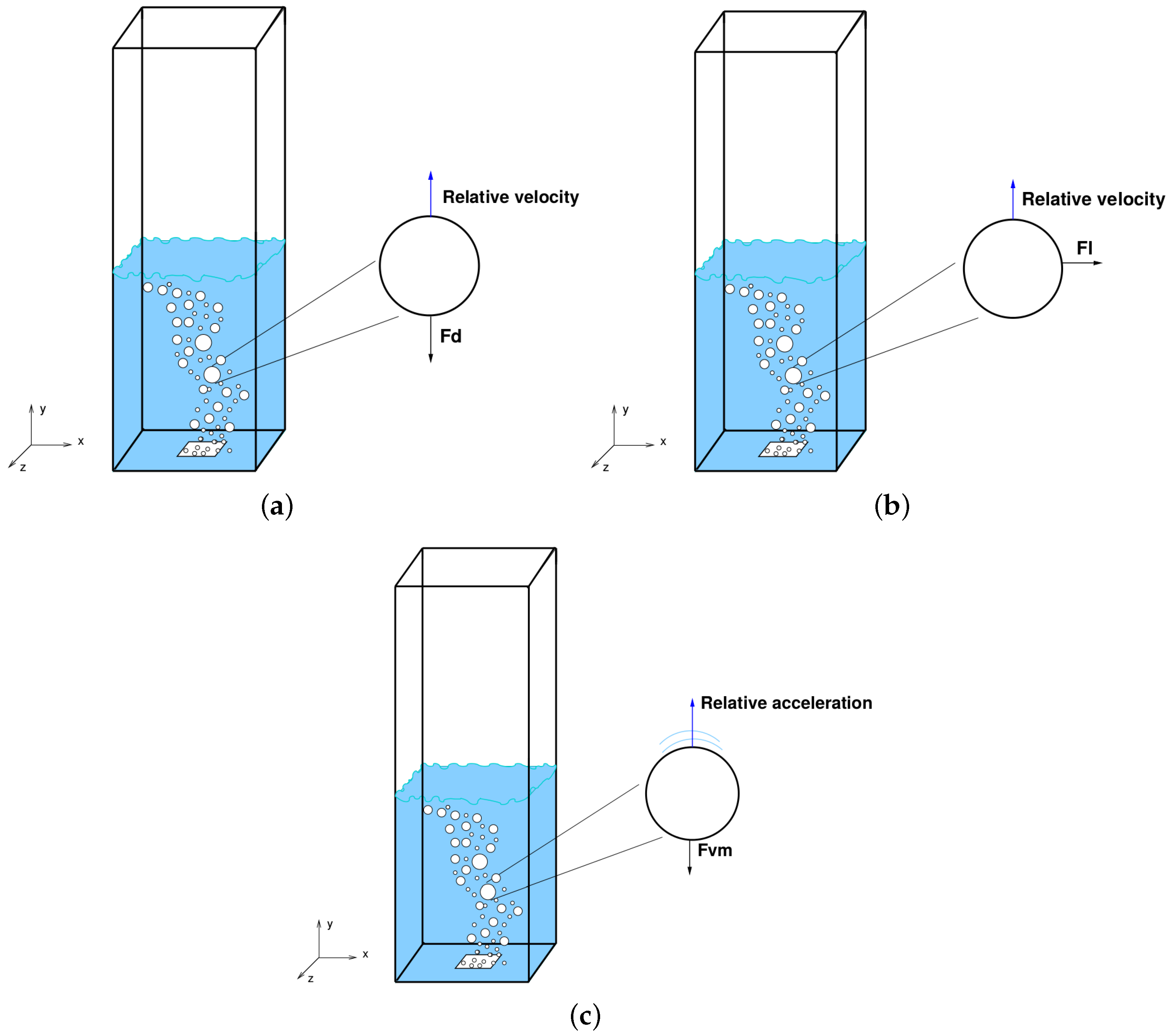
Illustrations of the three interfacial forces here considered are shown in schematic form in Figure 2, and a summary of the coefficients adopted for these forces is given in Table 3.
The Reynolds stress for phase i, needed in Equation (2), is given as:
where I is the identity tensor, the turbulent kinetic energy for phase i, and is the effective viscosity, composed of the following contributions:
where the subscriptions l, t and L refer, respectively, to laminar, turbulent and liquid phase.
The three k- turbulence models considered in this work calculate the effective viscosity in different ways. The standard k- model calculates exactly as written in Equation (10). The modified k- includes an additional term on the right-hand-side of the equation, accounting for the turbulence induced by the movement of the bubbles through the liquid. Here, this term follows the model proposed by Sato et al. [33]:
where is the bubble diameter (see Equation (35) below), the gas velocity, and the liquid velocity.
For both the standard and modified k- models, is defined as:
in which , k is the turbulent kinetic energy, and the rate of dissipation of the turbulent kinetic energy, calculated just for the liquid phase, as described by Equations (13) and (14) respectively:
where , , , , and stands for the production of turbulent kinetic energy defined, for example, as in Rusche [52]:
For the mixture k- equations, the turbulence variables are defined as mixture quantities of the two phases, and are calculated here for both the gas and liquid phases in the manner proposed by Behzadi et al. [53]:
The coefficients present in the mixture k- model are the same as for the standard k- model, while the mixture properties are defined as:
where
3.1. Population Balance Model (PBM)
In this work, we specifically consider the presence of different bubble diameters. The sizes may vary due to the coalescence and break-up processes occurring, caused by the liquid turbulence. We have adopted here the QMOM model of McGrow [18] to determine the bubble-size distribution.
Assuming that both coalescence and breakup processes may occur in the bubble column, the governing equation for the population balance (length-based) can be written, according to Marchisio et al. [14], as:
where is the length-based (L) number density function.
Applying the moment transformation and a quadrature approximation for the integral [18],
results in the following equation:
where the subscript refers to the order of each moment, varying from 0 up to (2N− 1), where N is the number of nodes considered in obtaining the weights and abscissae. The coefficients and are, respectively, the coalescence and breakage kernels, and denotes the daughter size distribution.
Note that specific details of the step-by-step derivation leading to Equation (26) can be found in the reference paper of Marchisio et al. [14].
The weights () and abscissae () in Equation (26) can be obtained through the product-difference approach [54] or Wheeler algorithm [55]; the first approach is adopted in the present work, since it results in a simpler implementation, and is said to be stable for and [56], which is our case here.
The total number of nodes used is N = 3, which then provides six moments [57]. Each moment (t) has different physical meaning depending on the order . For , is the total number of particles/bubbles; for , is the length of the particles/bubbles; for , is the surface area of the particles/bubbles; while for , gives the total particle/bubble volume [57].
The coalescence between two colliding bubbles, represented by the term containing the coefficient (also referred as the kernel) in Equation (26), can be expressed as the product of the collision frequency and the collision efficiency , in which and are the diameters of the two colliding bubbles, as follows:
The coalescence kernel used here is that proposed by Luo [41], which is based on the assumption of isotropic turbulence in the liquid phase [58]. This leads to a collision frequency of the following form:
where is the mean turbulent velocity of the bubbles (which should be related to the size of the turbulent eddies):
where , according to [41].
The collision efficiency given by Luo [41] is defined as the ratio between the coalescence time needed to annihilate the liquid film between the colliding bubbles to a critical rupture thickness, and to the interaction time between the two bubbles, as expressed below:
Luo [41] considered to be a function of Weber number (), and to be a function of the virtual mass coefficient , the physical properties, and the bubble size ratio. The final collision efficiency is then expressed as:
where , = and is the surface tension.
For the breakage kernel , we use that suggested by Luo and Svendesson [40], which has been widely applied before [13,23,59,60,61], and which calculates simultaneously the daughter distribution () according to the following prescription:
where assuming isotropic turbulence, is the size ratio between an eddy and a bubble in the inertial sub-range, and is defined as the increase coefficient of the surface area given by
in which is the breakage volume fraction, assumed here to be given by , to represent a symmetrical breakage.
The integration in Equation (32) can be performed by applying an incomplete gamma function approach, as shown in the work of Bannari et al. [23].
After calculating the kernels, the Sauter mean diameter (), which is needed in the momentum and turbulence equations (Equations (2) and (11)), can be obtained by dividing the third moment (bubble volume) and the second moment (bubble surface area), as suggested by Marchisio et al. [14]:
The initial values of the moments may be given by a Gaussian distribution of the density function, as found by Marchisio et al. [56], which results in the following values for the moments: , , , , and .
3.2. Validation and Verification
Verification and Validation are distinct assessment processes; both have been utilized in the present work to give a measure of confidence in the numerical results obtained. The AIAA [62] has produced a guideline document on verification and validation, in which one can easily appreciate the difference between the two.
In brief, verification is defined as the process to determine whether the mathematical equations have been solved correctly. Assurance of this is obtained by comparing numerical results against analytical data or against numerical data of higher accuracy. Validation is the process of determining the degree to which a model is an accurate representation of the physics, and this can only be achieved by comparison with actual experimental data; i.e., by a simulation featuring the same set-up, boundary conditions, materials and flow conditions of the experiment. The distinction between the two was succinctly stated by Roache [63] as: “verification is solving the equations right” (meaning correctly), “while validation is solving the right equations”.
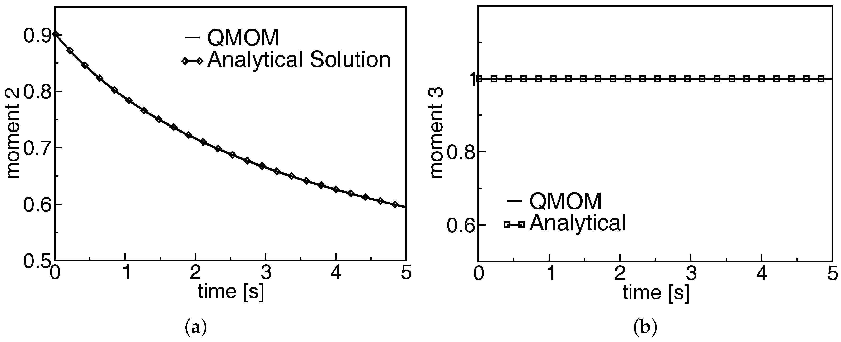
Therefore, before using the models for validation purposes, the QMOM equations implemented in the OpenFOAM code were first checked by comparing the moments obtained (Equation (26)) with the analytical solutions of Marchisio et al. [14]. As shown in Figure 3 and Figure 4, very good agreement was obtained, so the model was accepted as being correctly implemented for the further validation studies.
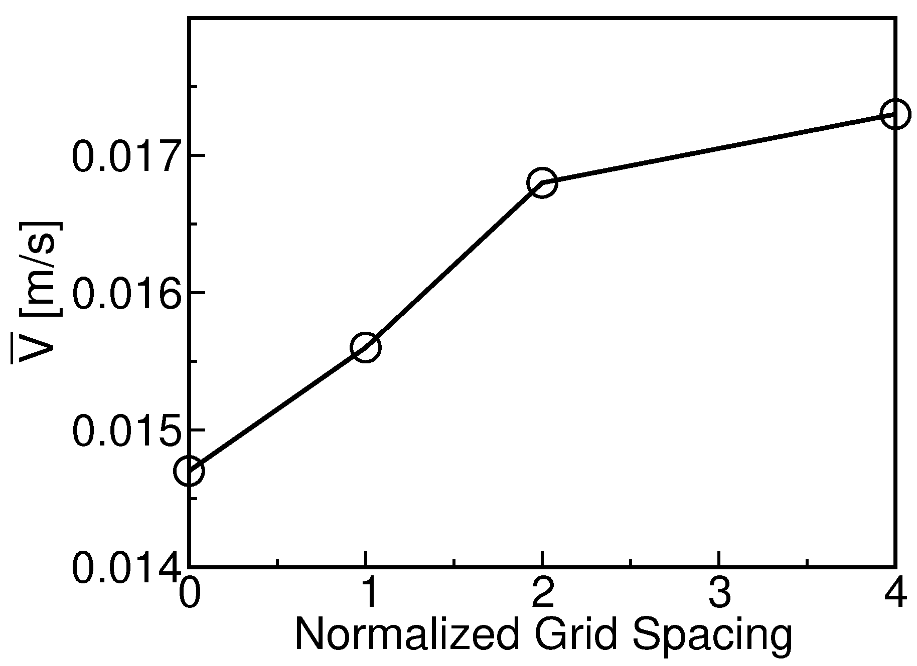
Part of the verification process in this paper includes the calculation error where a mesh sensitivity analysis is performed on the test-cases with same setup as the experiment (see Section 2). The time-step here selected is s and remains constant over the simulation time; it respects the CFL condition of Courant number < 1, provides low residuals, and small computational time.
3.3. Boundary Conditions
The geometry presented in Figure 1 features one inlet at the bottom (sparger), one outlet (top of the water column), and non-slip walls. The superficial gas velocities 0.0013, 0.0073 and 0.020 m/s represent the respective inlet velocities of the air, after multiplying each value by the cross-sectional area of the column and dividing by the sparger area. In the experiment, no liquid was injected with the gas (i.e., and at the inlet), so the inlet liquid velocity is set to zero in the calculation.
The inlet conditions for k and are calculated, respectively, as follows:
where , and I the turbulence intensity, assumed here to be standard (it was not measured), and
in which is the assumed initial eddy size, calculated as , where is a characteristic length, assumed to be the sparger width, and the constant is based on the maximum value of the mixing length in a fully-developed turbulent pipe flow [64,65].
For the outlet region, a switch between a Neumann condition (zero-gradient) for outflow and a Dirichlet condition for inflow is used for k, , , and . In OpenFOAM, that is imposed through the condition [66].
For pressure, a boundary condition that adjusts the gradient according to the flow is used for both the inlet and the walls (given by the name in OpenFOAM). A Dirichlet boundary condition is assigned for pressure at the outlet boundary, using a total pressure (atmospheric) of 1.01325 Pa.
The kernels (Equations (27) and (32)) are evaluated in each cell of the domain: so, for the inlet, the bubbles are assumed not to have any initial coalescence and breakage rates associated with them. For the outlet, and the walls, a zero-gradient condition is defined for both the coalescence and breakage kernels. The same is applied to the Sauter mean diameter, , on the walls and outlet, but at the inlet a fixed value (0.005 m) is assumed, which is the average bubble diameter found in the experiment of Pfleger et al. [22] being simulated here; the bubbles at inlet are assumed to be of spherical shape.
Wall functions are used to estimate k and in the viscous layer region near the wall, allowing [64,67,68].
Table 4 presents all the boundary conditions used in the simulations here discussed.
It is important to point out that the simulations with inlet air velocity greater than 0.0013 m/s are initialized using the values obtained from the last time-step of the simulation with the next lower inlet air velocity, to reduce the computational time to reach steady-state conditions.
3.4. Numerical Methods
All the simulations are performed using the the open-source CFD code OpenFOAM version 2.3.0. The PIMPLE algorithm, merged PISO [69] and SIMPLE [70], is used for the coupling between the velocity and pressure fields, as recommended by Rusche [52] for bubble-driven flows. Inside the PIMPLE loop, the momentum equation is solved using an initial guess for the pressure (Step 1). Then, at each time iteration, the pressure equation is solved twice with the velocity obtained from Step 1, and finally a corrector is applied to provide an updated value of the velocity based on the updated value of the pressure: this is continued to convergence. The procedure is repeated for each time step. The interested reader can obtain a more detailed explanation of the algorithm in Holzmann [71] and the OpenFOAM documentation [72].
A second-order-accurate, central-difference scheme (CDS) is used for the gradient and Laplacian terms in the governing equations, while a second-order-accurate, upwind scheme has been selected for the advection terms: this to ensure stability of the iteration. Time integration is performed using a second-order implicit backward method. The convergence criterion for all the cases is that the average residuals (for mass, pressure, velocity and turbulence variables) are less than .
The Euler-Euler two-phase solver is structured in such a way that first the momentum equations are solved inside the PIMPLE loop, then the turbulence quantities are calculated, and finally the PBM equation is solved to provide the Sauter mean diameter for the bubbles, which is then used in the next time-step to estimate the interfacial forces in the momentum (Equations (4) and (7)) and turbulence (Equations (11) and (23)) transport equations.
All the simulations are carried out with a constant time-step of 0.001 s, which ensures a Courant number () less than 1. For this criterion to be achieved, a mesh independence analysis has been performed, as explained in the next section. Under-relaxation factors () are used for pressure (), velocity (), () and (), in order to promote smooth convergence, especially for the test cases with higher superficial gas velocities (0.0073 m/s and 0.020 m/s).
Time-averaging in each simulation was taken over a period of 200 s, which was sufficient for the steady-oscillation regime to be achieved. Table 5 summarizes all the test cases featured in this work.
4. Results and Discussion
4.1. Mesh Sensitivity Study
A mesh sensitivity analysis has been performed for three mesh sizes, the details of which are specified in Table 6. The analysis was performed assuming a constant bubble size of 0.005 m, and with the standard k- turbulence model.
As shown in Table 6, the mesh refinement was undertaken in the transversal direction to the flow, plane xz (see Figure 1), in order to better capture the major velocity gradients, which are higher in this direction than axially, in accordance with the conclusions of Ziegenhein et al. [73] and Guédon et al. [5] in their mesh sensitivity studies.
Another important piece of information concerning the meshes it that, as discussed comprehensively by Milelli [74], an optimum ratio of the grid to the bubble diameter should be maintained of around 1.5, since larger values than this could lead to transfer of a large portion of the resolved, energy-containing scales into sub-grid-scale motion; hence in the present mesh sensitivity study a ratio less than 1.5 was specified in all cases.
The order of grid convergence (p) is here estimated based on the vertical water velocity component integrated over the column width (), as provided by each i-th mesh index (see Table 6), namely by:
where is the grid refinement ratio.
In order to calculate the theoretical asymptotic solution () for zero grid size, also known as the Richardson extrapolation method [75], the value of p calculated from Equation (38) is used in the following equation:
Another parameter useful in indicating the degree of mesh independence is the Grid Convergence Index (GCI), which is an estimate of the discretization error, and how far the solution is from its asymptotic value. For RANS computations, a GCI of less than 5% is considered acceptable [63,76]. According to Roache [63]:
Using , one can calculate the asymptotic range () of convergence:
which indicates if the solution is in the error band, ca ≈ 1 [77].
4.2. Influence of the Interfacial Forces on the Fluid Dynamics
For a better and more robust prediction of the flow patterns in a bubble column, and in two-phase flow simulations in general, an accurate description of the relevant interfacial forces is an absolute necessity. Therefore, before investigating the turbulence models in detail, the influence of the drag and lift forces on the fluid flow behaviour has first to be scrutinized. As concluded by Gupta and Roy [13], the virtual mass force does not greatly influence the fluid flow patterns for this kind of bubble column once the flow is established, so this effect has not been studied in detail in this paper.
Pourtousi et al. [47] have provided a comprehensive literature review on the topic of interfacial forces in bubble columns from which they concluded that, for the drag and lift coefficients, the most-used models are respectively those of Schiller and Naumann [48] and Tomiyama et al. [49], respectively. Consequently, this paper concentrates on these models for the prediction of the velocity and gas hold-up profiles.
It is important to point out that for the bubble-size range studied in this paper (≈0.005–0.0054 m), the Tomiyama et al. [49] coefficient in the lift force is positive, and acts to drive the bubbles towards the wall. For bubbles larger than a critical diameter (0.0058 m at atmospheric pressure), the opposite occurs, and the bubbles would move towards the center of the water column [78,79,80].
As shown in Figure 6a, a near-zero velocity is found at a distance less than 0.020 m from the wall. This situation occurs for downward flow direction close to the walls, which is not the case for the interior of the column. Later, Figure 11a will confirm this behavior.
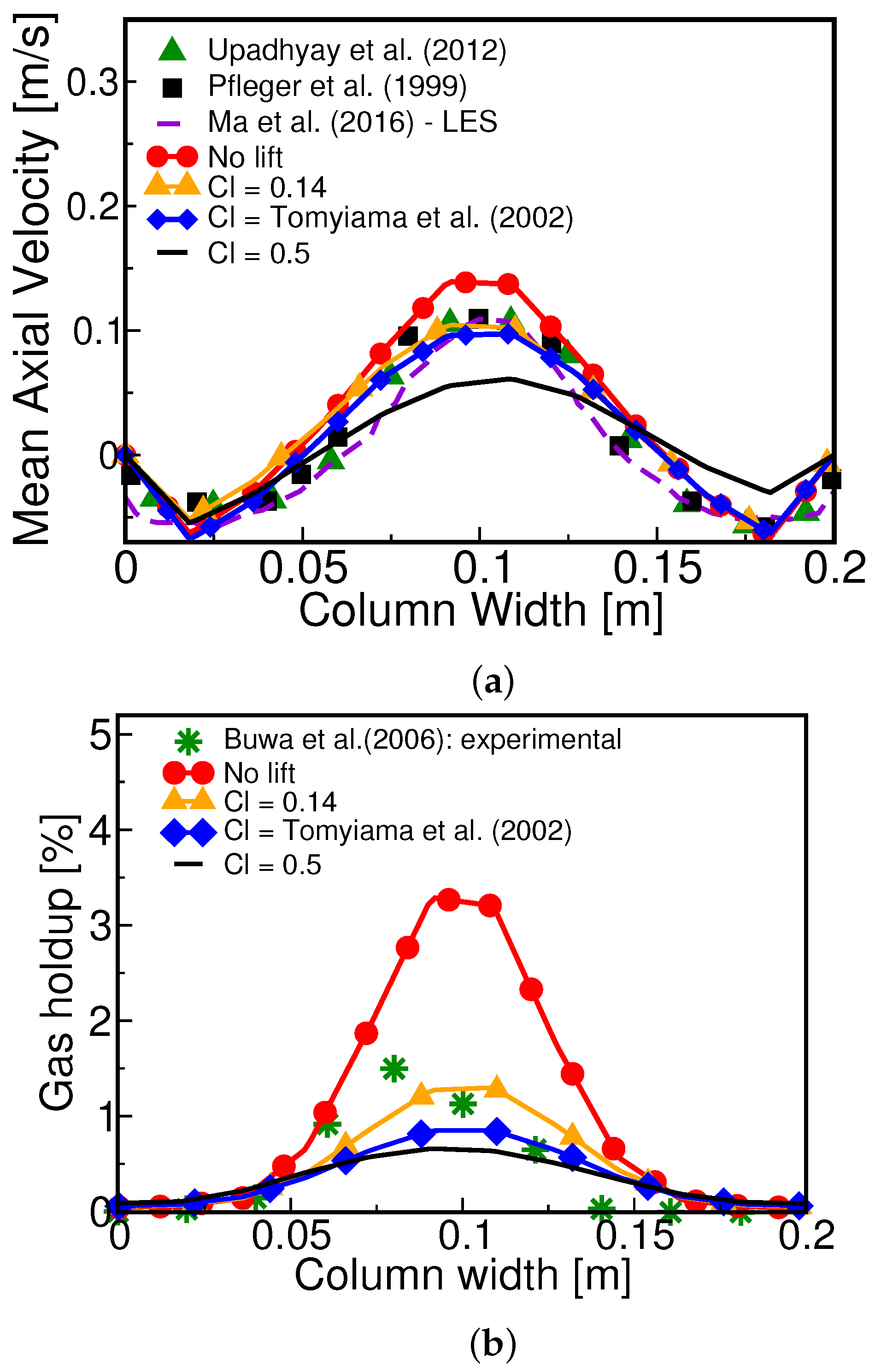
An interesting observation is that, for the velocity profiles, the combination of both models (Schiller and Naumann [48] for the drag coefficient and Tomiyama et al. [49] for the lift one) works well, providing good comparisons against data from different experiments, and from associated LES data: see Figure 6a. However, the same is not true for the gas hold-up: see Figure 6b. It is also important to note that the magnitude of the lift coefficient provided by the Tomiyama et al. [49] model is (similar observation was obtained by Kulkarni [81]). To test the sensitivity to this value, two further simulations were carried out using smaller () and higher () lift coefficients. In addition, one extra calculation is presented for which the lift force has been ignored completely, i.e., for which .
As can be seen in Figure 6, without the lift force there is no lateral force to encourage the bubbles to migrate towards the walls (in the absence of the turbulent diffusion force), hence both velocity and gas hold-up profiles are too peaked. Including a non-zero lift coefficient, the bubbles are seen to indeed migrate to the walls, and flatten the profiles, particularly so for the gas hold-up profile. A fixed lift coefficient of appears to be the optimum choice for this particular experiment.
Previous studies on the topic [8] presented some discrepancies between Tomiyama et al. lift force [49] and the experimental data, which were explained to be originated from the Wellek et al. correlation [50]. The latter was originally obtained for droplets in liquids [82] and it might not be suitable for the present poli-disperse bubbly flow [8,82,83].
In Figure 6b, the reason why their experimental data is shifted off-center, according to Buwa et al. [35], is due to the fact that, for the considered superficial gas velocity (0.0013 m/s), the bubble plume is narrow, and its oscillation period large, making it difficult to collect data over a sufficiently long time to obtain a symmetric gas hold-up profile. In the present work, the errors are within the range of the experimental uncertainties [35].
Therefore, we conclude that the lift force has an essential role to play on the prediction of the gas hold-up, which, in comparison to that of the vertical water velocity, is much more sensitive to the choice of lift coefficient.
4.3. Influence of the Turbulence Model on the Hydrodynamics
In addition to the interfacial forces, turbulence modelling is an important component in the accurate prediction of the flow patterns in bubble columns. The most used turbulence model, in two-phase flows is still the k- model, due to its simplicity and the low computational effort [46,47]. For this reason, in this paper, we have studied the turbulence in the context of three variants of the k- model: standard, modified and mixture. The purpose here is to reach some conclusion on which choice provides better agreement with experimental data, at least in the context of the present application.
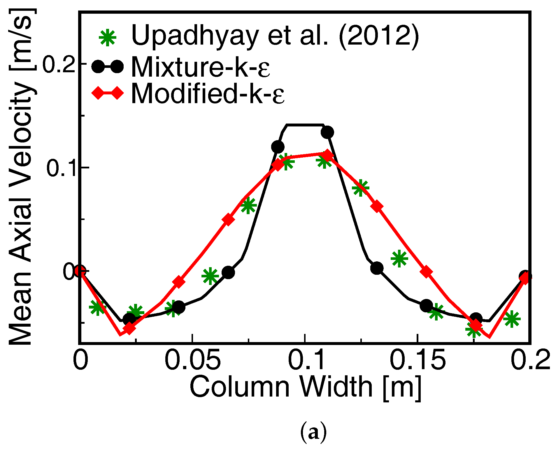
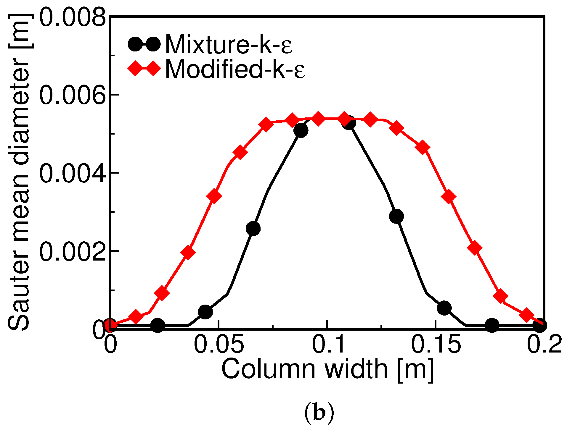
It transpires that both the standard and modified k- models produce similar profiles for axial velocity, gas hold-up and Sauter mean diameter. However, the same is not true for the mixture k- model, as shown in Figure 7a.
One can also observe that for all the turbulence models, the profile of the bubble size distribution can be explained by the effect of the lift force, which enhances the movement of larger bubbles towards the center of the bubble column, and the smaller bubbles towards the walls, resulting in a parabolic shape of the size distribution for the considered superficial gas velocity (0.0013 m/s). A similar conclusion was reached in the experimental work performed by Besagni and Inzoli [84]. As it will be shown in the Section 4.4, as the superficial gas velocity increases, the recirculation of the flow becomes more intense, causing a spread of the bubbles all over the domain (even far from the sparger), and consequently a more homogeneous bubble size distribution (see Figure 10d and Figure 12b).
Turbulent boundary conditions affect the results mostly on the bottom wall close to the sparger, where as discussed by Ekambara et al. [24], the flow is more anisotropic and requires different modeling such as Reynolds Stress Model (RSM) and Large Eddy Simulation (LES). Away from the sparger the numerical solutions given by isotropic turbulence models, such as the k- model, proves to have a good agreement with the experimental data [24,29,35].
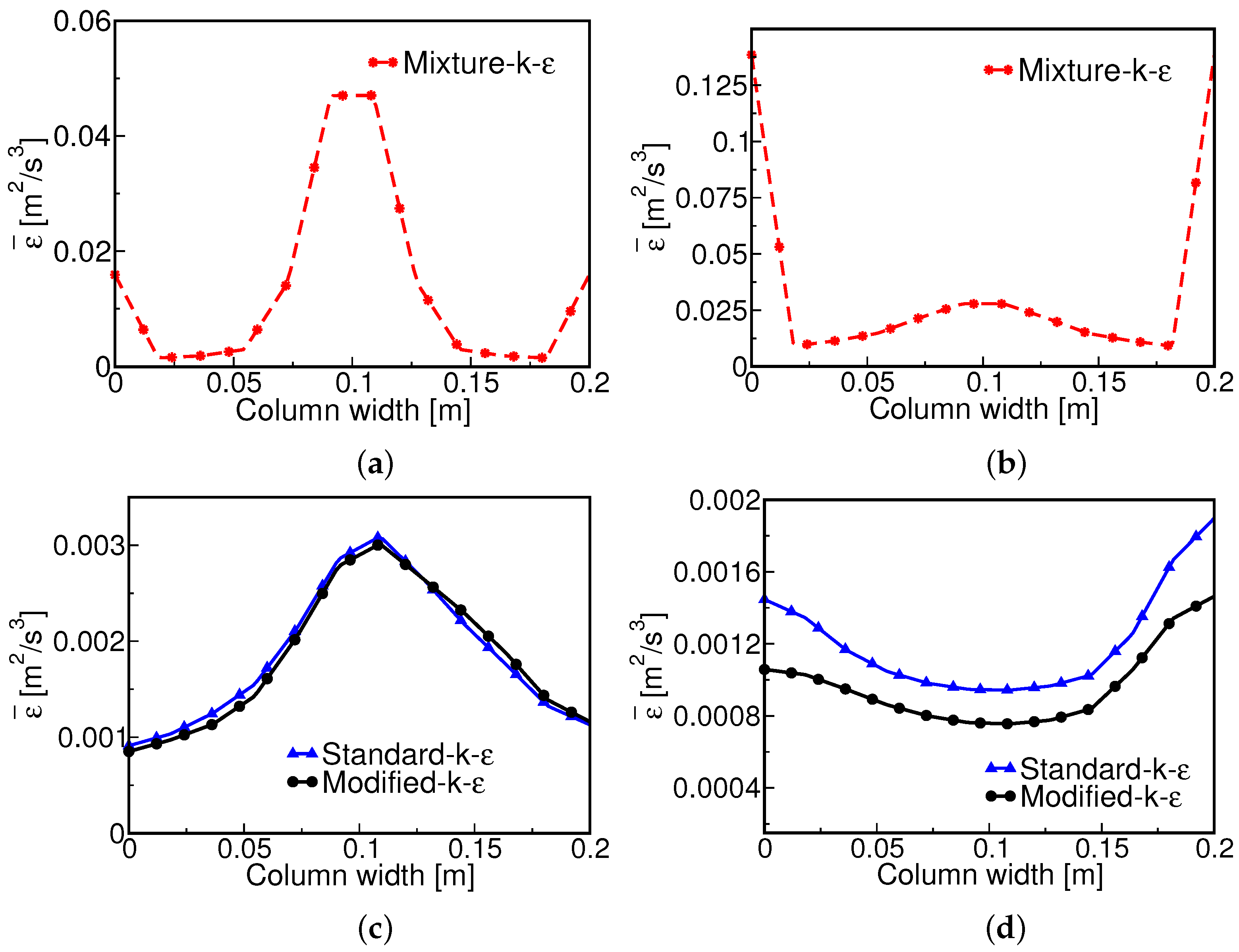
Figure 8 shows the profiles of the time-averaged turbulent dissipation rate () in two different regions: one close to the sparger (y = 0.13 m), and the other close to the liquid/gas interface (y = 0.37 m). As can be observed, near the sparger (Figure 8a,c) the higher values of occur in the central region, for all the turbulence models here studied, as a direct consequence of the turbulence created by the insertion of bubbles into the water column.
However, in quantitative terms, the mixture k- model predicts to be one order of magnitude higher than those of the other two models in the region near the sparger. This can be explained by the high influence the model has in respect to the gas volume fraction through the ratio of the dispersed phase velocity fluctuations to the continuous phase fluctuations, as represented by the coefficient : see the variable definitions below Equation (23). This ratio is used in the model to obtain for each phase.
According to Behzadi et al. [53], for bubbly flows for which (such as for water-air flows), the mixture turbulence equations tend to those of the continuous phase alone, except in regions where ≈ 1, as happens very near the sparger, explaining the behavior of in Figure 8a, but not elsewhere.
In the region close to the upper water level, where flow recirculation is a predominant mechanism, higher values of occur near the wall, and the difference between the mixture and the other k- models is even more evident (Figure 8b,d), suggesting this model is not the most adequate for a deeper analyses of this kind of bubble column.
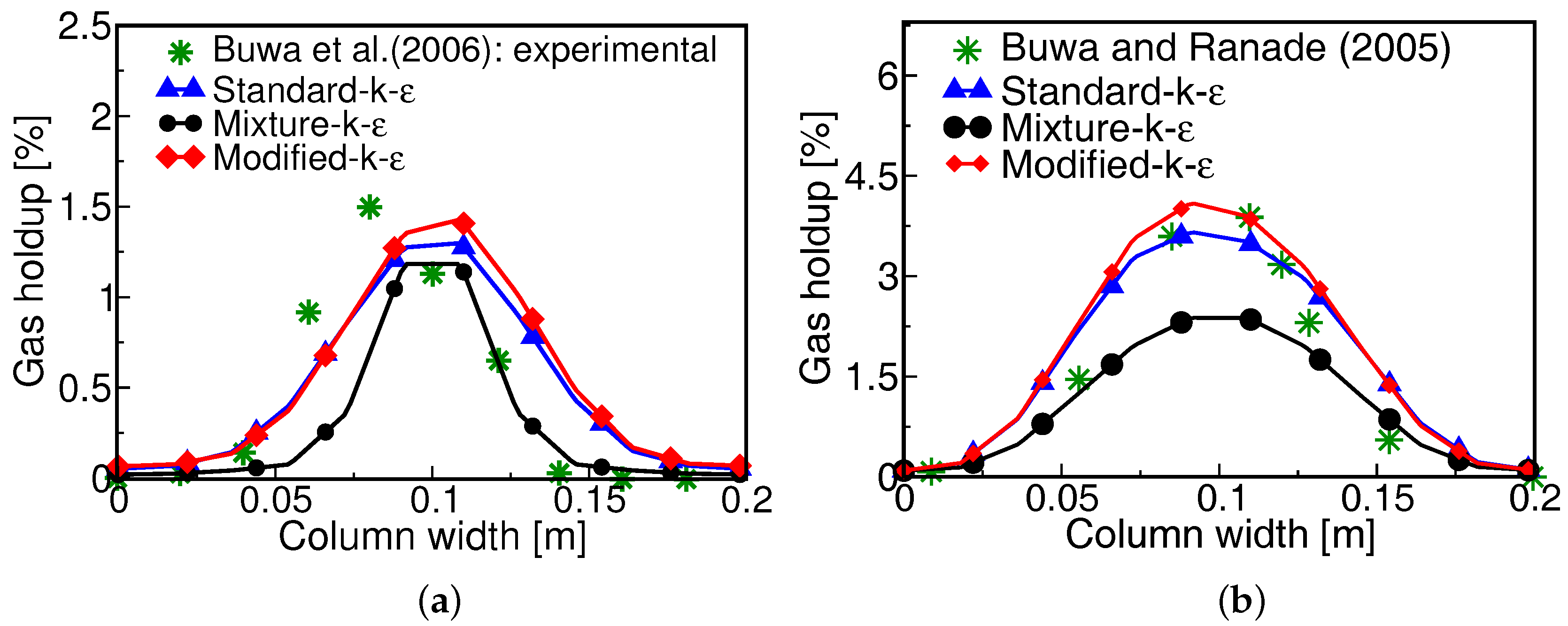
The high values of provided by the mixture k- model near the sparger, which as a consequence dissipates more effectively the bubbles over the height of the water column, is also reflected in under-prediction of the gas hold-up, as depicted in Figure 9. The results shown in Figure 9a,b are from different test-cases, and taken at different positions, for validation purposes, once the experiments (depicted by green stars in the graphs) were obtained by different superficial gas velocities, at different locations in the bubble column.
It is worth noting that if one is only interested in obtaining velocity profiles of the continuous phase, the mixture k- model could be used with some confidence (as can be seen in Figure 7a). The same does not hold for the gas hold-up, which is the variable highly affected by the over-prediction of the turbulent kinetic energy dissipation rate, as shown in Figure 9.
4.4. Influence of the Air Superficial Gas Velocity at Inlet on the Fluid Behavior
As well as the specification of the interfacial forces and the turbulence modeling, the superficial gas velocity at the inlet plays an important role on the predicted hydrodynamics of the bubbles in the column. To study this influence, three different air injection velocities have been investigated: UG = 0.0013, 0.0073 and 0.02 m/s. It is to be noted that none of these generate turbulent eddies with enough energy to induce bubble break-up, as observed for UG = 0.03 m/s [85]. Consequently, we focus here on the fluid dynamics for conditions under which coalescence is the dominant bubble interaction phenomenon; discussion of results for the UG = 0.03 m/s case is reserved for future work.
Figure 10 shows the gas hold-up and Sauter mean diameter profiles for two different regions of the water column, for three superficial gas velocities. As can be observed, near the sparger (y = 0.02 m) there is a higher concentration of bubbles, albeit in a narrow region, resulting in similar behavior for the bubble size distribution for all the three superficial air inlet velocities. Figure 10d shows that, for UG = 0.02 m/s, the bubbles are predicted to be of uniform size across the width of the column, and reach the top with a higher probability of interaction with each other in the central region due to the higher population density there (Figure 10c).
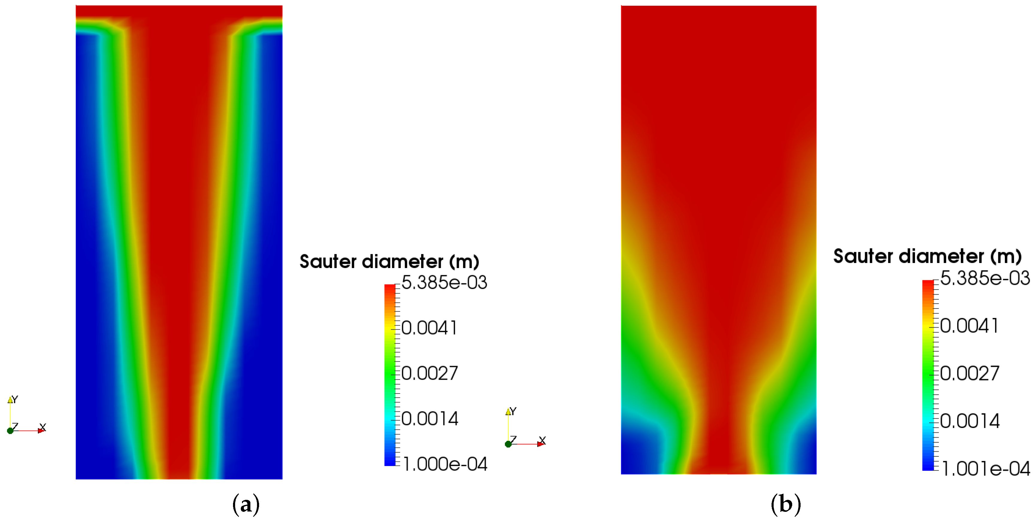
Figure 11a shows downward flow along both walls and upward flow in the bulk region. A rotational pattern can also be observed in the middle of the column, which is stronger in the lower half of the column. This flow pattern can help explaining the fact of 0.0054-m bubbles staying in the centre region of the column, as depicted by Figure 12a. A downward flow along the left wall and on the lower portion of the right column wall can be discerned in Figure 11b, as well as a strong upward flow in the middle of the lower portion of the column, which tends to drift towards the upper-left wall. This cross-mixing behaviour may explain why the 0.0054-m bubbles spread throughout the upper portion of the column as shown by Figure 12b.
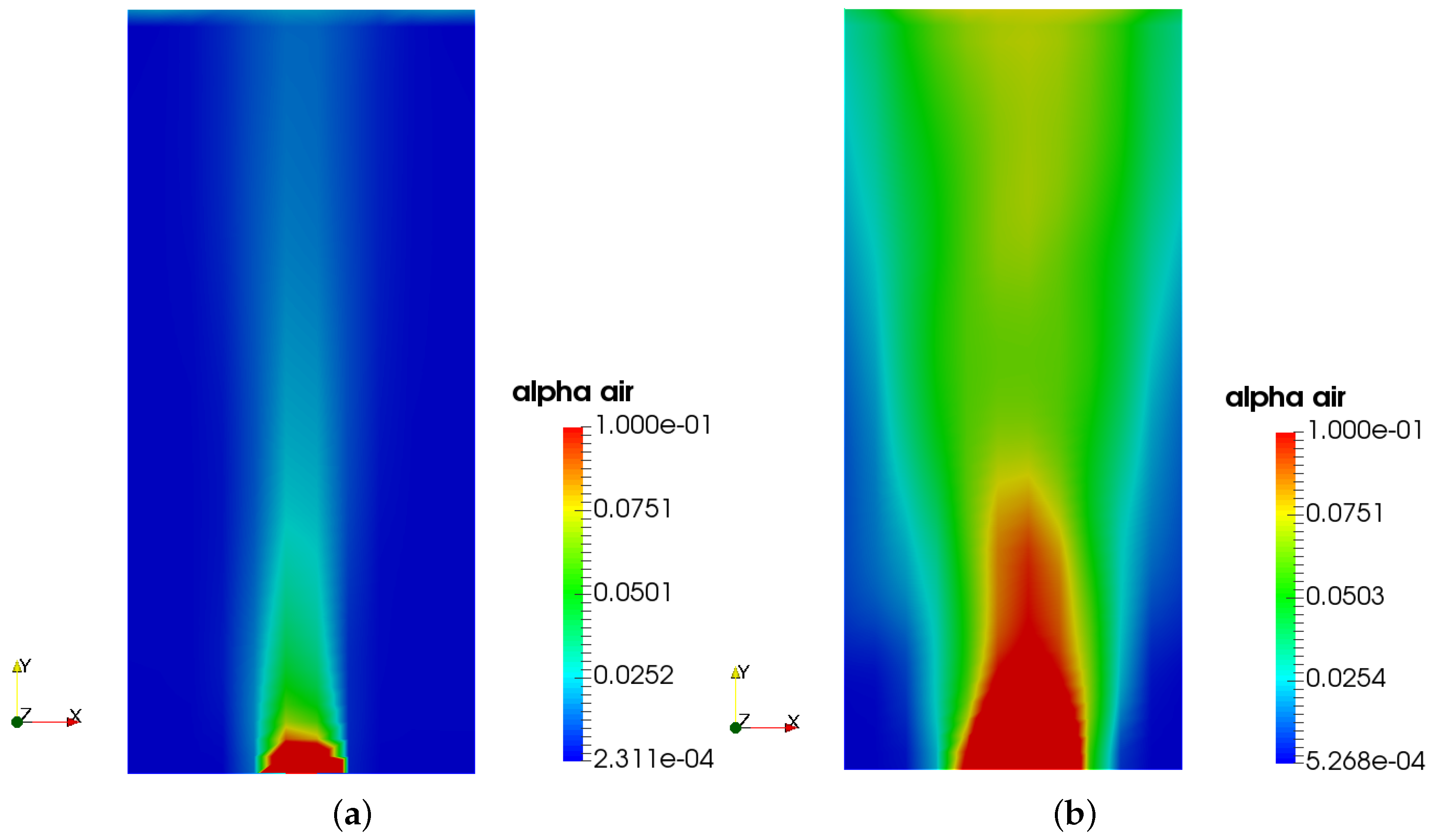
Figure 13a,b show, in shaded contour form, the behavior of the bubble volume fraction inside the water column, for UG = 0.0013 and 0.02 m/s. The greater axial velocity and stronger recirculation provided by the UG = 0.02 m/s case (Figure 11b), results in a wider spread of the bubbles across the column (Figure 13b).
For the superficial gas velocity highlighted here (UG = 0.02 m/s), the coalescence kernel (that of Luo [41]) is driven by the collision frequency ( in Equation (28)), this is, in regions where is non-negligible the frequency of bubble coalescence is more predominant than the collision efficiency (), which is proportional to the mean turbulent velocity as seen in Equation (31). A similar observation was made by Deju et al. [59], who studied different combination of coalescence and breakup kernels in a circular rather than square bubble column. In their study, they found that the collision frequency diminishes when the eddy dissipation rate becomes insignificant at the centre of the bubble column, while the opposite occurs in respect to the collision efficiency: both calculations incorporated the model proposed by Prince and Blanch [85] for the coalescence kernel.
For the given superficial gas velocities adopted in this work, a bi-dispersed model, as that proposed by Guédon et al. [5], proved to be a very good alternative to the use of a population balance model. However, if one is interested in capturing the size distribution of the bubbles, and understanding the phenomena that take place in the evolution of the bubble sizes, specially for higher inlet velocities (>0.04 m/s), use of population balance approach is recommended [85].
5. Conclusions
A hydrodynamic investigation of two-phase flow, with different spherical bubble size distributions, in a scaled-up rectangular bubble column geometry using CFD has been presented. Three parameters are identified as playing important roles on the fluid dynamics for this kind of flow: the gas/liquid interfacial forces, the liquid turbulence, and the superficial gas velocity at inlet.
From our examination of the interfacial forces, it is concluded that, though the use of the bubble lift force suggested by Tomiyama et al. [49] has resulted in reasonable comparisons of vertical water velocity compared with the experimental data, the same is not true for the measured gas hold-up, at least for the cases investigated here. In fact, a constant lift coefficient () proved to be the most suitable choice for better axial velocity and gas hold-up comparisons with experimental data. The lift force formulation is seen to have had a strong effect on the prediction of the gas hold-up, and consequently on the bubble size profiles, at different locations in the bubble column.
Concerning turbulence modeling, the mixture k- model predicted much higher turbulent kinetic dissipation rates, combined with lower values of gas volume; other variants of the k- model perform better. From the k- turbulence models here investigated, the modified k- model proved to be a good compromise between modeling simplicity and accuracy of predictions.
It is seen that the superficial gas velocity at inlet (UG) has an important influence on the characteristics of the fluid dynamics in the bubble column, and ultimately on the bubble size distribution within it. By increasing UG, there is an increase in the gas hold-up, even near the upper interface of the liquid, resulting in a more uniform bubble-size distribution throughout the column.
More work is needed for cases with higher injection velocities than those considered here, for which few experimental data are currently available from the point of view of deciding on the turbulence modeling approaches.
Acknowledgments
The authors are very grateful for the support given by the Chemical Engineering Department of the Université de Sherbrooke, Canada and in terms of a fellowship award.
Author Contributions
Camila Braga Vieira has implemented some of the equations used in the simulations in OpenFOAM, has also implemented the Modified k-ε turbulence model by including the additional terms in the existing k-ε turbulence model, performed all the simulations and analyses, and written the paper. Giuliana Litrico has helped at the post-processing stage for the graphical display of the results, has participated in the discussion of the results, and has reviewed the paper. Ehsan Askari has helped with part of implementation of the equations in OpenFOAM. Gabriel Limieux has also helped in the implementation stage, and Professor Pierre Proulx has given his overall supervision, helped with the analysis of the results, and contributed to the additional knowledge required for the execution of this work.
Conflicts of Interest
The authors declare no conflict of interest.
Nomenclature
| Sauter mean diameter [m] | |
| G | gas |
| H | height of the cavity [m] |
| I | turbulence intensity |
| k | turbulent kinetic energy [m/s] |
| l | laminar |
| eddy size [m] | |
| L | liquid |
| characteristic length [m] | |
| friction velocity: | |
| mean velocity vector [m/s] | |
| W | column width [m] |
| w | water phase |
| dimensionless wall distance: | |
| Greek symbols | |
| phase volume fraction | |
| dissipation rate of turbulent kinetic energy [m/s] | |
| molecular kinematic viscosity [m/s] | |
| turbulent kinematic viscosity [m/s] | |
| specific mass [kg/m] | |
| surface tension [N/m] | |
| shear stress [kg/(m·s)] | |
| Acronyms | |
| CFL | Courant–Friedrichs–Lewy condition |
| LES | Large Eddy Simulation |
| PBM | Population Balance Model |
| PIMPLE | merged Piso-sIMPLE algorithm |
| QMOM | Quadrature Method of Moments |
| RSM | Reynolds Stress Model |
References
- Degaleesan, S.; Dudukovic, M.; Pan, Y. Experimental study of gas-induced liquid-flow structures in bubble columns. AIChE J. 2001, 47, 1913–1931. [Google Scholar] [CrossRef]
- Becker, S.; De Bie, H.; Sweeney, J. Dynamic flow behaviour in bubble columns. Chem. Eng. Sci. 1999, 54, 4929–4935. [Google Scholar] [CrossRef]
- Lain, S.; Broder, D.; Sommerfeld, M. Experimental and numerical studies of the hydrodynamics in a bubble column. Chem. Eng. Sci. 1999, 54, 4913–4920. [Google Scholar] [CrossRef]
- Kantarci, N.; Borak, F.; Ulgen, K. Bubble column reactors. Process Biochem. 2005, 40, 2263–2283. [Google Scholar] [CrossRef]
- Guédon, G.; Besagni, G.; Inzoli, F. Prediction of gas-liquid flow in an annular gap bubble column using a bi-dispersed Eulerian model. Chem. Eng. Sci. 2017, 161, 138–150. [Google Scholar] [CrossRef]
- Shnip, A.; Kolhatkar, R.; Swamy, D.; Joshi, J. Criteria for the transition from the homogenous to the heterogeneous regime in two-dimensional bubble column reactors. Int. J. Multiph. Flow 1992, 18, 705–726. [Google Scholar] [CrossRef]
- Krishna, R.; van Baten, J. Mass transfer in bubble columns. Catal. Today 2003, 79–80, 67–75. [Google Scholar] [CrossRef]
- Besagni, G.; Inzoli, F.; Ziegenheim, T.; Lucas, D. Computational fluid-dynamics modeling of the pseudo-homogeneous flow regime in large-scale bubble columns. Chem. Eng. Sci. 2016, 160, 144–160. [Google Scholar] [CrossRef]
- Vijayan, M.; Schlaberg, H.; Wang, S. Effects of sparger geometry on the mechanism of flow pattern transition in a bubble column. Chem. Eng. J. 2007, 130, 171–178. [Google Scholar] [CrossRef]
- Upadhyay, R.; Roy, S.; Pant, H. Benchmarking radioactive particle tracking (RPT) with Laser Doppler Anemometry (LDA). Int. J. Chem. React. Eng. 2012, 10. [Google Scholar] [CrossRef]
- Upadhyay, R.; Pant, H.; Roy, S. Liquid flow patterns in rectangular ait-water bubble column investigated with radioactive particle tracking. Chem. Eng. Sci. 2013, 96, 152–164. [Google Scholar] [CrossRef]
- Liu, Y.; Hinrichsen, O. Study on CFD-PBM turbulence closures based on k-ε and Reynolds stress models for heterogeneous bubble column flows. Comput. Fluids 2014, 105, 91–100. [Google Scholar] [CrossRef]
- Gupta, A.; Roy, S. Euler-euler simulation of bubbly flow in a rectangular bubble column: Experimental validation with radioactive particle tracking. Chem. Eng. J. 2013, 225, 818–836. [Google Scholar] [CrossRef]
- Marchisio, D.; Vigil, R.; Fox, R. Quadrature method of moments for aggregation-breakage processes. J. Colloid Interface Sci. 2003, 258, 322–334. [Google Scholar] [CrossRef]
- Ramkrishna, D. Population Balances; Academic Press: San Diego, CA, USA, 2000. [Google Scholar]
- Kumar, S.; Ramkrishna, D. On the solution of population balance equations by discretization ii—A moving pivot technique. Chem. Eng. Sci. 1996, 51, 1333–1342. [Google Scholar] [CrossRef]
- Smith, M.; Matsoukas, T. Constant number Monte Carlo simulation of population balances. Chem. Eng. Sci. 1998, 53, 1777–1786. [Google Scholar] [CrossRef]
- McGrow, R. Description of Aerosol Dynamics by the Quadrature Method Moments. Aerosol Sci. Technol. 1997, 27, 255–265. [Google Scholar] [CrossRef]
- Rong, F.; Marchisio, D.; Fox, R. Application of direct quadrature method of moments to polydisperse gas solid fluidized beds. Powder Technol. 2004, 139, 7–20. [Google Scholar]
- Aboulhasanzadeh, B.; Thomas, S.; Taeibi-Rahni, M.; Tryggvason, G. Multiscale computations of mass transfer from buoyant bubbles. Chem. Eng. Sci. 2012, 75, 456–467. [Google Scholar] [CrossRef]
- Tryggvason, G.; Dabiri, S.; Aboulhasanzadeh, B.; Lu, J. Multiscale considerations in direct numerical simulations of multiphase flows. Phys. Fluids 2013, 25, 031302. [Google Scholar] [CrossRef]
- Pfleger, D.; Gomes, S.; Gilbert, N.; Wagner, H.G. Hydrodynamic simulations of laboratory scale bubble columns fundamental studies of the Eulerian-Eulerian modeling approach. Chem. Eng. Sci. 1999, 54, 5091–5099. [Google Scholar] [CrossRef]
- Bannari, R.; Kerdouss, F.; Selma, B.; Bannari, A.; Proulx, P. Three-dimensional mathematical modeling of dispersed two-phase flow using class method of population balance in bubble columns. Comput. Chem. Eng. 2008, 32, 3224–3237. [Google Scholar] [CrossRef]
- Ekambara, K.; Dhotre, M. CFD simulation of bubble column. Nucl. Eng. Des. 2010, 240, 963–969. [Google Scholar] [CrossRef]
- Buwa, V.; Ranade, V. Characterization of gas-liquid flows in rectangular bubble columns using conductivity probes. Chem. Eng. Commun. 2005, 192, 1129–1150. [Google Scholar] [CrossRef]
- Murgan, I.; Bunea, F.; Ciocan, G.D. Experimental PIV and LIF characterization of a bubble column flow. Flow Meas. Instrum. 2017, 54, 224–235. [Google Scholar] [CrossRef]
- Borchers, O.; Busch, C.; Sokolichin, A.; Eigenberger, G. Applicability of the standard k-ε turbulence model to the dynamic simulation of bubble columns. Part II: Comparison of detailed experiments and flow simulations. Chem. Eng. Sci. 1999, 54, 5927–5935. [Google Scholar] [CrossRef]
- Mudde, R.F.; Simonin, O. Two- and three-dimensional simulations of a bubble plume using a two-fluid model. Chem. Eng. Sci. 1999, 54, 5061–5069. [Google Scholar] [CrossRef]
- Becker, S.; Sokolichin, A.; Eigenberger, G. Gas liquid flow in bubble columns and loop reactors: Part ii. Comparison of detailed experiments and flow simulations. Chem. Eng. Sci. 1994, 49, 5747–5762. [Google Scholar] [CrossRef]
- Van Thai, D.; Minier, J.; Simonin, O.; Freydier, P.; Olive, J. Multidimensional two-fluid model computation of turbulent dispersed two-phase flows. In Numerical Methods in Multiphase Flows; ASME: New York, NY, USA, 1994; Volume FED 185, pp. 277–291. [Google Scholar]
- Li, G.; Yang, X.; Dai, G. CFD simulation of effects of the configuration of gas distributors on gas-liquid flow and mixing in a bubble column. Chem. Eng. Sci. 2009, 64, 5104–5116. [Google Scholar] [CrossRef]
- Chen, J.; Li, F.; Degaleesan, S.; Gupta, P.; Al-Dahhan, M.; Dudukovic, M.; Toseland, B. Fluid dynamic parameters in bubble columns with internals. Chem. Eng. Sci. 1999, 54, 2187–2197. [Google Scholar] [CrossRef]
- Sato, Y.; Sadatomi, M.; Sekoguchi, K. Momentum and heat transfer in two-phase bubble flow theory. Int. J. Multiph. Flow 1975, 7, 167–177. [Google Scholar] [CrossRef]
- Kulkarni, A.; Ekambara, K.; Joshi, J. On the development of flow pattern in a bubble column reactor: Experiments and CFD. Chem. Eng. Sci. 2007, 62, 1049–1072. [Google Scholar] [CrossRef]
- Buwa, V.; Deo, D.; Ranade, V. Eulerian-lagrangian simulations of unsteady gas-liquid flows in bubble columns. Int. J. Multiph. Flow 2006, 32, 864–885. [Google Scholar] [CrossRef]
- Rampure, M.; Kulkarni, A.; Ranade, V. Hydrodynamics of bubble column reactors at high gas velocity: Experiments and computational fluid dynamics (CFD) simulations. Ind. Eng. Chem. Res. 2007, 46, 8431–8447. [Google Scholar] [CrossRef]
- Zhang, D.; Deen, N.; Kuipers, J. Numerical simulation of the dynamic flow behavior in a bubble column: A study of closures for turbulence and interface forces. Chem. Eng. Sci. 2006, 61, 7593–7608. [Google Scholar] [CrossRef]
- Deen, N. An Experimental and Computational Study of Fluid Dynamics in Gas-Liquid Chemical Reactor. Ph.D. Thesis, Aalborg University, Esbjerg, Denmark, 2001. [Google Scholar]
- Ma, T.; Ziegehein, T.; Lucas, D.; Frohlich, J. Large eddy simulation of the gas-liquid flow in a rectangular bubble column. Nucl. Eng. Des. 2016, 299, 146–153. [Google Scholar] [CrossRef]
- Luo, H.; Svendsen, H. Theoretical model for drop and bubble breakup in turbulent dispersions. AIChE J. 1996, 42, 1225–1233. [Google Scholar] [CrossRef]
- Luo, H. Coalescence, Breakup and Liquid Circulation in Bubble Column Reactor. Ph.D. Thesis, The Norwegian Institute of Technology, Trondheim, Norway, 1993. [Google Scholar]
- Saffman, P.; Turner, J. On the collision of drops in turbulent clouds. J. Fluid Mech. 1956, 1, 16–30. [Google Scholar] [CrossRef]
- Hagesather, L.; Jakobsen, H.; Hjarbo, K.; Svendsen, H. A coalescence and breakup module for implementation in CFD codes. Comput. Aided Chem. Eng. 2000, 8, 367–372. [Google Scholar]
- Versteeg, H.; Malalasekera, W. An Introduction to Computational Fluid Dynamics; Longman Scientific and Technical: Harlow, UK, 2011. [Google Scholar]
- Sato, Y.; Sekoguchi, K. Liquid velocity distribution in two-phase bubble flow. Int. J. Multiph. Flow 1975, 2, 79–95. [Google Scholar] [CrossRef]
- Tabib, M.V.; Roy, S.A.; Joshi, J.B. CFD simulation of bubble column—An analysis of interphase forces and turbulence models. Chem. Eng. J. 2008, 139, 589–614. [Google Scholar] [CrossRef]
- Pourtousi, M.; Sahu, J.; Ganesan, P. Effect of interfacial forces and turbulence models on predicting flow pattern inside the bubble column. Chem. Eng. Process. 2014, 75, 38–47. [Google Scholar] [CrossRef]
- Schiller, L.; Naumann, Z. A drag coefficient correlation. Z. Vereins Deutsch. Ing. 1935, 77, 318–320. [Google Scholar]
- Tomiyama, A.; Tamai, H.; Zun, I.; Hosokawa, S. Transverse migration of single bubbles in simple shear flows. Chem. Eng. Sci. 2002, 57, 1849–1858. [Google Scholar] [CrossRef]
- Wellek, R.; Agrawal, A.; Skelland, A. Shape of liquid drops moving in liquid media. AIChE J. 1966, 12, 854–862. [Google Scholar] [CrossRef]
- Odar, F.; Hamilton, W. Forces on a sphere accelerating in a viscous fluid. J. Fluid Mech. 1964, 18, 302–314. [Google Scholar] [CrossRef]
- Rusche, H. Computational Fluid Dynamics of Dispersed Two-Phase Flows at High Phase Fractions. Ph.D. Thesis, Imperial College of Science, Technology and Medicine, London, UK, 2002. [Google Scholar]
- Behzadi, A.; Issa, R.; Rusche, H. Modelling of dispersed bubble and droplet flow at high phase fractions. Chem. Eng. Sci. 2004, 59, 759–770. [Google Scholar] [CrossRef]
- Gordon, R. Error bounds in equilibrium statistical mechanics. J. Math. Phys. 1968, 9, 655–663. [Google Scholar] [CrossRef]
- Sack, R.; Doovan, A. An algorithm for Gaussian quadrature given modified moments. Numer. Math. 1971, 18, 465–478. [Google Scholar]
- Marchisio, D.; Fox, R. Computational Models for Polydisperse Particulate and Multiphase Systems; Cambridge University Press: New York, NY, USA, 2013. [Google Scholar]
- Su, J.; Gu, Z.; Li, Y.; Feng, S.; Xu, Y. Solution of population balance equation quadrature method of moments with an adjustable factor. Chem. Eng. Sci. 2007, 62, 5897–5911. [Google Scholar] [CrossRef]
- Hinze, J. Turbulence; McGraw-Hill: New York, NY, USA, 1959. [Google Scholar]
- Deju, L.; Cheung, S.; Yeoh, G.; Qi, F.; Tu, J. Comparative analysis of coalescence and breakage kernels in vertical gas-liquid flow. Can. J. Chem. Eng. 2015, 93, 1295–1309. [Google Scholar] [CrossRef]
- Sanya, J.; Marchisio, D.; Fox, R.; Kumar, D. On the comparison between population balance models for CFD simulation of bubble columns. Ind. Eng. Chem. Res. 2005, 44, 5063–5072. [Google Scholar] [CrossRef]
- Wang, T.; Wang, Y.; Jin, Y. Population balance model gas-liquid flows: influence of bubble coalescence and breakup models. Ind. Eng. Chem. 2005, 44, 7540–7549. [Google Scholar] [CrossRef]
- AIAA. AIAA Guide for the Verification and Validation of Computational Fluid Dynamics Simulations; AIAA Report G-077-1988; American Institute of Aeronautics and Astronautics: Reston, VA, USA, 1998. [Google Scholar]
- Roache, P. Verification and Validation in Computational Science and Engineering; Hermosa Publishers: Socorro, NM, USA, 1998; pp. 358–359. [Google Scholar]
- Wilcox, D. Turbulence Modeling for CFD; DCW Industries Inc.: La Cañada Flintridge, CA, USA, 1993. [Google Scholar]
- Schetz, J.A.; Fuhs, A. Fundamentals of Fluid Mechanics; John Wiley and Sons Inc.: Hoboken, NJ, USA, 1999. [Google Scholar]
- User Guide; OpenFOAM-User Guide Version 4.0; OpenFOAM Foundation: London, UK, 2016; pp. 140–141.
- Chieng, C.; Launder, B. On the calculation of turbulent heat transport downstream from an abrupt pipe expansion. J. Numer. Heat Transf. 1980, 3, 189–207. [Google Scholar]
- Craft, T.; Launder, B.; Suga, K. Development and application of a cubic eddy-viscosity model of turbulence. Int. J. Heat Fluid Flow 1996, 17, 108–115. [Google Scholar] [CrossRef]
- Issa, R. Solution of implicitly discretized fluid flow equations by operator-splitting. J. Comput. Phys. 1986, 62, 40–65. [Google Scholar] [CrossRef]
- Patankar, S. Numerical Heat Transfer and Fluid Flow; Series in Computational Methods in Mechanics and Thermal Sciences; Taylor and Francis: Milton Park, Didcot, UK, 1980. [Google Scholar]
- Holzmann, T. Mathematics, Numerics, Derivations and OpenFOAM(R), 4th ed.; Holzmann CFD: Leoben, Austria, 2016; pp. 108–128. [Google Scholar]
- OpenFOAM. OpenFOAM Guide The PIMPLE Algorithm in OpenFOAM; OpenFOAM: London, UK, 2016. [Google Scholar]
- Ziegenhein, T.; Rzehak, R.; Lucas, D. Transient simulation for large scale flow in bubble columns. Chem. Eng. Sci. 2015, 122, 1–13. [Google Scholar] [CrossRef]
- Milelli, M. A Numerical Analysis of Confined Turbulent Bubble Plume. Diss. ETH No. 14799. Ph.D. Thesis, Swiss Federal Institute of Technology Zurich, Zurich, Switzerland, 2002; pp. 4146–4157. [Google Scholar]
- Richardson, L. The approximate arithmetical solution by finite differences of physical problems involving differential equations, with application to the stresses in a masonry dam. Philos. Trans. R. Soc. Lond. 1911, 210, 307–357. [Google Scholar] [CrossRef]
- Roache, P.J. Perspective: A method for uniform reporting of grid refinement studies. J. Fluids Eng. 1994, 116, 405–413. [Google Scholar]
- Slater, J. Examining Spatial (Grid) Convergence. Available online: http://www.grc.nasa.gov/WWW/wind/valid/tutorial/spatconv.html (accessed on 5 January 2018).
- Lucas, D.; Prasser, H.M.; Manera, A. Influence of the lift force on the stability of a bubble column. Chem. Eng. Sci. 2005, 60, 3609–3619. [Google Scholar]
- Lucas, D.; Krepper, E.; Prasser, H.M.; Manera, A. Investigations on the stability of the flow characteristics in a bubble column. Chem. Eng. Technol. 2006, 29, 1066–1072. [Google Scholar] [CrossRef]
- Lucas, D.; Krepper, E.; Prasser, H.M. Use of models for lift, wall and turbulent dispersion forces acting on bubbles for poly-disperse flows. Chem. Eng. Sci. 2007, 62, 4146–4157. [Google Scholar] [CrossRef]
- Kulkarni, A. Lift force on bubbles in a bubble column reactor: Experimental analysis. Chem. Eng. Sci. 2008, 63, 1710–1723. [Google Scholar] [CrossRef]
- Besagni, G.; Inzoli, F. Bubble size distributions and shapes in annular gap bubble column. Exp. Therm. Fluid Sci. 2016, 74, 27–48. [Google Scholar] [CrossRef] [Green Version]
- Besagni, G.; Inzoli, F.; Ziegenhein, T.; Dirk, L. The pseudo-homogeneous flow regime in large-scale bubble columns: Experimental benchmark and computational fluid dynamics modeling. Petroleum 2017. [Google Scholar] [CrossRef]
- Besagni, G.; Inzoli, F. The effect of liquid phase properties on bubble column fluid dynamics: Gas holdup, flow regime transition, bubble size distributions and shapes, interfacial areas and foaming phenomena. Chem. Eng. Sci. 2017, 170, 270–296. [Google Scholar] [CrossRef]
- Prince, M.; Blanch, H. Bubble coalescence and break-up in air-sparged bubble columns. AIChE J. 1990, 36, 1485–1499. [Google Scholar] [CrossRef]
Figure 1.
Sketch of the bubble column configuration: the sparger is located at the centre of the bottom face, as in the experimental facility of Pfleger et al. [22].
Figure 1.
Sketch of the bubble column configuration: the sparger is located at the centre of the bottom face, as in the experimental facility of Pfleger et al. [22].

Figure 2.
Schematic illustration of the interfacial forces modeled: (a) drag; (b) lift and (c) virtual mass.
Figure 2.
Schematic illustration of the interfacial forces modeled: (a) drag; (b) lift and (c) virtual mass.

Figure 3.
Verification of QMOM equations by comparison with the analytical solution provided by Marchisio et al. [14]: (a) time history of moment 0 and (b) its respective time-history error.
Figure 3.
Verification of QMOM equations by comparison with the analytical solution provided by Marchisio et al. [14]: (a) time history of moment 0 and (b) its respective time-history error.
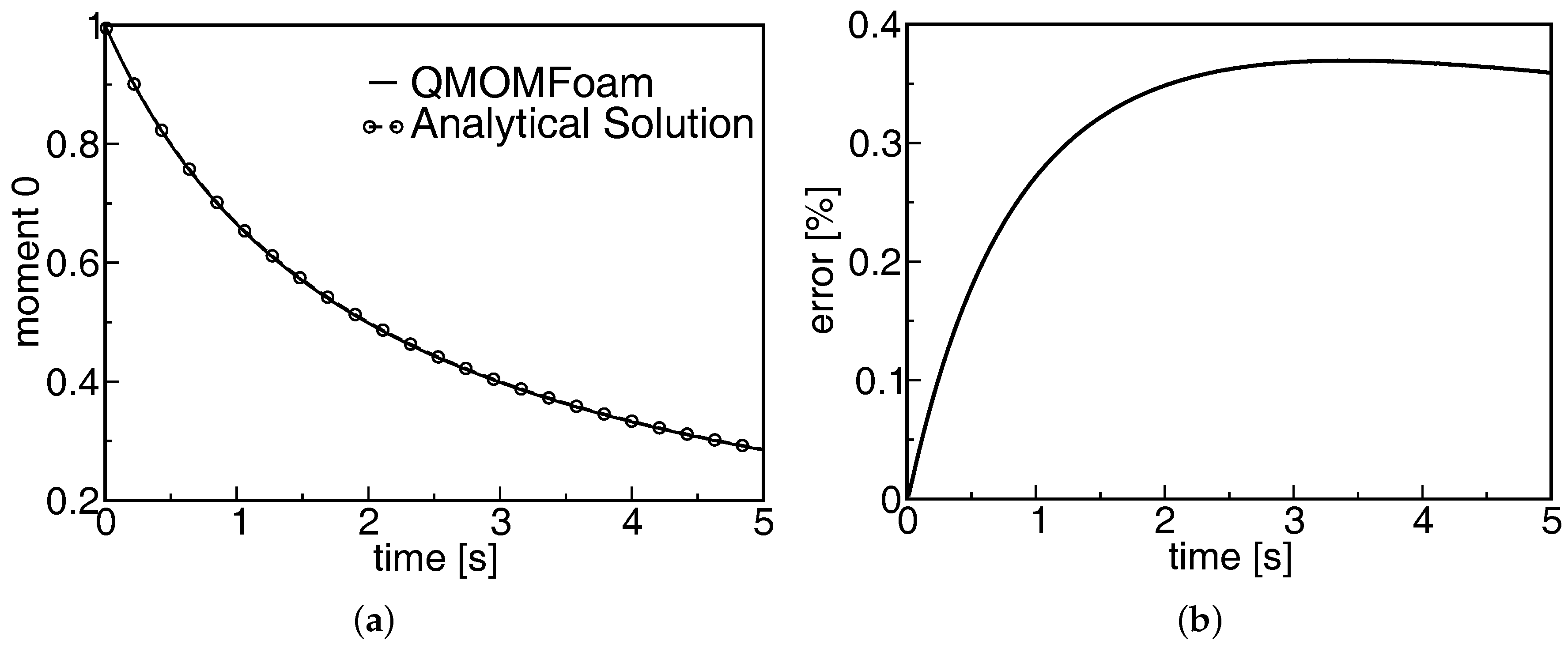
Figure 4.
Verification of the moments used in the calculation of : (a) time history of moment 2, (b) time history of moment 3, by comparison with analytical solution provided by Marchisio et al. [14].
Figure 4.
Verification of the moments used in the calculation of : (a) time history of moment 2, (b) time history of moment 3, by comparison with analytical solution provided by Marchisio et al. [14].

Figure 5.
Asymptotic averaged-axial-water-velocity behavior for a normalized grid spacing tending to zero.
Figure 5.
Asymptotic averaged-axial-water-velocity behavior for a normalized grid spacing tending to zero.

Figure 6.
(a) Axial mean water velocity profile at y = 0.25 m; and (b) gas hold-up profiles at y = 0.37 m for the case UG = 0.0013 m/s from various sources. All the results have been obtained using the modified k- model, and are represented by the line with circles (No lift), the joined triangles (), diamonds ( Tomiyama et al. [49] ), and the straight line (0.5).

Figure 7.
(a) Time-averaged water vertical velocity profile at y = 0.25 m and (b) Sauter mean diameter at y = 0.37 m as provided by the mixture and modified k- turbulence models, for a superficial gas velocity of 0.0013 m/s at inlet.
Figure 7.
(a) Time-averaged water vertical velocity profile at y = 0.25 m and (b) Sauter mean diameter at y = 0.37 m as provided by the mixture and modified k- turbulence models, for a superficial gas velocity of 0.0013 m/s at inlet.


Figure 8.
Time-averaged profiles of across the column width at (a); (c) y = 0.13 m and (b); (d) at y = 0.37 m, for a superficial gas velocity at inlet of 0.0013 m/s.
Figure 8.
Time-averaged profiles of across the column width at (a); (c) y = 0.13 m and (b); (d) at y = 0.37 m, for a superficial gas velocity at inlet of 0.0013 m/s.

Figure 9.
Time-averaged gas hold-up along the column width at (a) y = 0.37 m and at (b) y = 0.21 m, for superficial gas velocities of 0.0013 m/s and 0.0073 m/s, respectively.
Figure 9.
Time-averaged gas hold-up along the column width at (a) y = 0.37 m and at (b) y = 0.21 m, for superficial gas velocities of 0.0013 m/s and 0.0073 m/s, respectively.

Figure 10.
Time-averaged of gas hold-up (left) and Sauter mean diameter (right) provided by Modified k- model at (a,b) y = 0.02 m and (c,d) y = 0.37 m.
Figure 10.
Time-averaged of gas hold-up (left) and Sauter mean diameter (right) provided by Modified k- model at (a,b) y = 0.02 m and (c,d) y = 0.37 m.

Figure 11.
Time-averaged water velocity field with instantaneous water velocity vectors provided by the Modified k- model after 100 s of simulation at (a) 0.0013 m/s; and (b) 0.02 m/s.
Figure 11.
Time-averaged water velocity field with instantaneous water velocity vectors provided by the Modified k- model after 100 s of simulation at (a) 0.0013 m/s; and (b) 0.02 m/s.
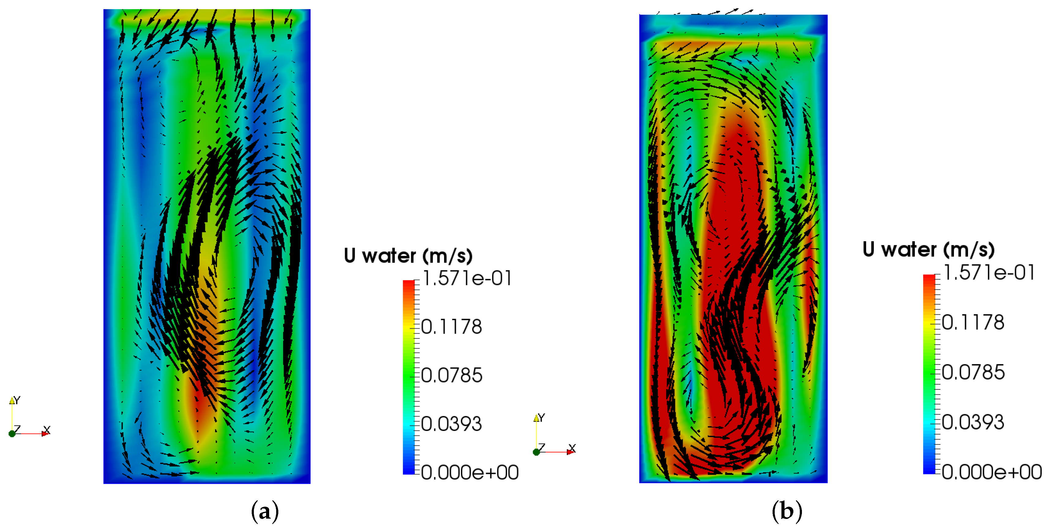
Figure 12.
Time-averaged Sauter diameter provided by the Modified k- model at (a) 0.0013 m/s; and (b) 0.02 m/s.
Figure 12.
Time-averaged Sauter diameter provided by the Modified k- model at (a) 0.0013 m/s; and (b) 0.02 m/s.

Figure 13.
Time-averaged gas hold-up provided by the Modified k- model for UG = (a) 0.0013 m/s; and (b) 0.02 m/s.
Figure 13.
Time-averaged gas hold-up provided by the Modified k- model for UG = (a) 0.0013 m/s; and (b) 0.02 m/s.

Table 1.
Summary of experimental works of turbulent flows in bubble columns.
| Author | Geometry (in m) | Air Inlet | Main Data Provided |
|---|---|---|---|
| Pfleger et al. [22] | Rectangular (H = 1.20, FH = 0.45, W = 0.20, D = 0.05) | 0.0013 m/s | Turbulent kinetic energy × Column depth; Vertical fluid velocity × Column width |
| Buwa and Ranade [25] | Rectangular with same dimensions of [22] | 0.0016–0.12 m/s | Time-averaged gas hold-up × Column width |
| Upadhyay et al. [10] | Rectangular with same dimensions of Pfleger et al. [22] | 0.0013 m/s | Mean axial velocity × Column width; Total kinetic energy × Column width |
| Upadhyay et al. [11] | Rectangular with same dimensions of Pfleger et al. [22] | 0.0013, 0.00833, 0.0125 m/s | Mean z-component velocity × Column width; Turbulent kinetic energy × Column width |
| Becker et al. [2] | Rectangular (FH = 0.45, W = 0.20, D = 0.04), cylindrical (FH = 2.5, Di = 0.295) | 0.0017 m/s (rectangular column), 0.0015–0.01 m/s (cylindrical) | Axial velocity × Time, at different locations. |
| Murgan et al. [26] | Rectangular (H = 1.10, W = 0.30, D = 0.30) | 0.000133 m/s | Water and bubble velocity fields; Bubble ascension velocity; diameter and interfacial area of bubbles. |
| Borchers et al. [27] | Rectangular (H = 2.0, W = 0.50, D = 0.08) | 0.0000167 m/s, 0.000033 m/s | Time series of the vertical velocity component at different locations. |
Geometry dimensions: H = height, FH = Fluid height, W = width, D = depth, Di = diameter.
Table 2.
Summary of numerical works of turbulent flows in bubble columns with and without bubble-size-distribution modelling.
Table 2.
Summary of numerical works of turbulent flows in bubble columns with and without bubble-size-distribution modelling.
| Author | Geometry | Interfacial Forces | Bubble Diameter | PBM Kernels | Turbulence Models | Remarks |
|---|---|---|---|---|---|---|
| Mude and Simonin [28] | Rectangular column [29]; = 0.20 m/s | D-Vm | 0.003 m | - | k- [30] and low-k- | No significant discrepancy on the results were found between the turbulence models investigated. |
| Li et al. [31] | Cylindrical column [32]; = 0.10 m/s; | D-L-Vm-WL-TD | Class method | Break: L-S; Coal: P-B | Modified-k- [33] | The configuration and location of gas distributor affects the overall gas hold-up and bubble sizes. |
| Ekambara and Dhotre [24] | Cylindrical column [34]; = 0.02 m/s | D-L-Vm | 0.006 m | - | k-, standard k-, RSM, RNG-k-, LES | RSM and LES provided a better prediction near the sparger, where the flow is more anisotropic. |
| Buwa et al. [35] | Rectangular column [22]; = 0.0016 m/s–0.12 m/s | D-L | 0.005 m | - | Standard k- | Satisfactory performance of Euler-Euler, with lift force, was found. |
| Liu and Hinrichsen [12] | Cylindrical column [36]; = 0.10 m/s–0.12 m/s | D-L | Class Method | Break: L-S; Coal: L | Modified-k- [33] and RSM | Tomyiana lift provided better agreement with experimental data, for both k- and RSM. |
| Zhang et al. [37] | Rectangular column [38]; = 0.0049 m/s | D-L-Vm | 0.004 m | - | Sub-grid scale model and different k- | The lift force strongly influences the bubble plume dynamics, and Tomiyana lift coefficient provided better results. |
| Bannari et al. [23] | Rectangular column [22]; = 0.0014 m/s and 0.0073 m/s | D-L-Vm | Class Method | Break: L-S; Coal: S-T and H | k- [28] | Good agreement with experimental data was found when using PBM for the bubble size. |
| Ma et al. [39] | Rectangular column [22]; = 0.0013 m/s | D-L-Vm | 0.002 m | - | LES | Good agreement with experimental data. |
Table 3.
Coefficients of the interfacial forces used in the present work and the respective models employed.
Table 3.
Coefficients of the interfacial forces used in the present work and the respective models employed.
| Interfacial Force | Model |
|---|---|
| Drag () | Schiller and Naumann [48] |
| Lift () | Tomiyama et al. [49] and Constant (0.14 and 0.5) |
| Virtual mass () | Constant (0.5) |
Table 4.
Boundary conditions for all the variables involved in the simulations of the bubble column here studied.
Table 4.
Boundary conditions for all the variables involved in the simulations of the bubble column here studied.
| Variable | Inlet | Outlet | Walls |
|---|---|---|---|
| k | Equation (36) | ||
| Equation (37) | |||
| p | |||
Table 5.
Summary of all the cases investigated by this work.
| UG (m/s) | Parameters Studied | Results |
|---|---|---|
| 0.0013 | Interfacial forces (Section 4.2) | Mean axial velocity (validation) |
| gas hold-up (validation) | ||
| 0.0013 and 0.0073 | Turbulence model (Section 4.3) | Mean axial velocity (UG = 0.0013 m/s) |
| profiles (UG = 0.0013 m/s) | ||
| profiles (UG = 0.0013 m/s) | ||
| gas hold-up (both UGs) | ||
| 0.0013, 0.0073 and 0.02 | Inlet gas velocity (Section 4.4) | gas hold-up profiles |
| profiles and fields | ||
| Water velocity fields |
Table 6.
Details of the meshes used in the sensitivity analysis.
| Mesh Index (i) | Number of Cells | ( m) | (m/s) | Normalized Grid Space |
|---|---|---|---|---|
| 1 | 11,800 | 108 | 0.0173 | 4 |
| 2 | 21,120 | 54 | 0.0168 | 2 |
| 3 | 42,240 | 27 | 0.0156 | 1 |
* ; ** = area of the cells along the side walls in the plane.
Table 7.
Convergence criteria used for choosing the appropriate mesh for the further simulations.
| r | p | ca | ||
|---|---|---|---|---|
| 2 | 1.26 | 2.6 | 6.4 | 1.028 |
© 2018 by the authors. Licensee MDPI, Basel, Switzerland. This article is an open access article distributed under the terms and conditions of the Creative Commons Attribution (CC BY) license (http://creativecommons.org/licenses/by/4.0/).
Share and Cite
MDPI and ACS Style
Braga Vieira, C.; Litrico, G.; Askari, E.; Lemieux, G.; Proulx, P. Hydrodynamics of Bubble Columns: Turbulence and Population Balance Model. ChemEngineering 2018, 2, 12. https://doi.org/10.3390/chemengineering2010012
AMA Style
Braga Vieira C, Litrico G, Askari E, Lemieux G, Proulx P. Hydrodynamics of Bubble Columns: Turbulence and Population Balance Model. ChemEngineering. 2018; 2(1):12. https://doi.org/10.3390/chemengineering2010012
Chicago/Turabian StyleBraga Vieira, Camila, Giuliana Litrico, Ehsan Askari, Gabriel Lemieux, and Pierre Proulx. 2018. "Hydrodynamics of Bubble Columns: Turbulence and Population Balance Model" ChemEngineering 2, no. 1: 12. https://doi.org/10.3390/chemengineering2010012