Study of Pressure Drop in Fixed Bed Reactor Using a Computational Fluid Dynamics (CFD) Code

Chemical Engineering Department, Baha’i Institute for Higher Education (BIHE), Tehran, Iran
*
Author to whom correspondence should be addressed.
ChemEngineering 2018, 2(2), 14; https://doi.org/10.3390/chemengineering2020014
Submission received: 28 November 2017
/
Revised: 1 March 2018
/
Accepted: 23 March 2018
/
Published: 2 April 2018
(This article belongs to the Special Issue Chemical Kinetics and Computational Fluid Dynamics Applied to Chemical Reactors Analysis and Design)
Abstract
:Pressure drops of water and critical steam flowing in the fixed bed of mono-sized spheres are studied using SolidWorks 2017 Flow Simulation CFD code. The effects of the type of bed formation, flow velocity, density, and pebble size are evaluated. A new equation is concluded from the data, which is able to estimate pressure drop of a packed bed for high particle Reynolds number, from 15,000 to 1,000,000.
1. Introduction
1.1. Fixed Bed Description and Applications
In the chemical, metallurgical, and nuclear industries, packed beds, also called fixed beds, are used extensively [1]. A fixed-bed reactor is based on a container filled with randomly formed stationary particles. Just to name some usages of fixed beds in different industries, the following applications could be mentioned: wastewater treatment processes, air purification, carbon dioxide recovery from flue gases, solvent or hydrocarbon vapor recovery distillation of vapor–liquid mixtures, immobilized enzymes and immobilized microbial cells, nitrogen oxide removal from power station flue gases, automobile exhaust purification, and in design of gas-cooled nuclear reactors, such as pebble-bed nuclear reactors or water-cooled reactors, such as Fixed Bed Nuclear Reactor (FBNR) [2,3,4,5,6].
Another application is packed liquid–liquid extraction towers, which give differential contacts, not stage contacts, and mixing and settling proceed continuously and simultaneously. In an extraction tower, there is continuous transfer of material between phases, and the composition of each phase changes as it flows through the tower; equilibrium is not reached at any given level, so there is always a departure from equilibrium which provides the driving force for mass transfer [7].
The advantages of fixed bed systems in relation to heat transfer are the high rates of heat transfer due to high turbulence existing in such systems, which results in higher convective heat transfer coefficients [7].
1.2. Pressure Drop Evaluation (Experimental and Computational)
In a fixed-bed system, the most importance parameter is the pressure drop of the fluid that penetrate the bed. The most conclusive way to determine pressure drop through a fixed bed is to perform experiment on the real system. Since constructing the real system is too expensive, normally experiments are performed on an experimental model representing the real system. This entails creating a suitable geometry, pumping fluid through the media, and using manometers to measure the pressure drop. This traditional method is also a relatively time-and money-consuming procedure. There exist technical difficulties of measuring flow parameters inside the fixed beds, making it difficult to be cognizant of the phenomena that occurs inside the bed, which could be studied with special technique, such as magnetic resonance imaging (MRI) and computed tomography (CT), etc. These drawbacks encourage finding an alternative way to deal with fixed beds, namely computational fluid dynamics (CFD) [8].
A large number of correlations can be found in the literature for the calculation of pressure drop resulting from fluid flowing through fixed beds. A review paper, published by Erdim in 2015, studied a total of 38 correlations from the literature, established a uniform notation to facilitate the comparison, and has evaluated them with experiments. A detailed presentation of these correlations are found in the abovementioned article [9].
In general, the pressure drop is a function of parameters, such as bed characteristics; i.e., bed height, particle diameter, porosity, and its distribution, and fluid characteristics, such as viscosity, density, and velocity. The equation published by Ergun about sixty years ago remains the most popular and the most widely-quoted pressure drop—flow rate relation for fluid flow through fixed beds, but it is only applicable for relatively low Reynolds (Re) number (Re < 1000) [1]. Ergun suggested relationship is in form of
in which is the fractional void volume, the gravitational constant, the diameter of the solid particles, superficial fluid velocity measured at average pressure, µ absolute viscosity of fluid, and mass flow rate of fluid ( [10].
KTA method is another famous equation to predict pressure drop, established by Kerntechnischer Ausschuss (KTA) in 1981, especially for a gas cooled fixed-bed reactor, and its focus is on applicability on higher range of Reynolds numbers. In the literature, it has been mentioned that the experimental results confirmed the validity of KTA equation up to [11]. Its original form is
where the coefficient of loss of pressure through friction is determined in accordance with the following empirical correlation [12]:
By substituting term 3 in the main formula, and changing to , the equation becomes
In the digital age, CFD has become a viable alternative to empirical methods. CFD is a branch of fluid mechanics that is capable to solve flow and energy balances in complicated geometries numerically; endless growth in computer capacity ensures that CFD is one of the fastest growing tools used in computer aided engineering design (CAE). Its popularity has stemmed from the relatively low set-up cost and man-hours compared to a full empirical study, coupled with the generally accepted accuracy of CFD. In addition, far more data, such as instantaneous pressure and velocity fields, could be extracted from CFD than its empirical counterpart [8]. Commercially available CFD codes use one of three basic spatial discretization methods, finite difference (FD), finite volume (FV), or finite element (FE) [13]. FD is a differential scheme that is approximation of a Taylor series expansion, bringing in some approximation errors. FV and FE methods are integral schemes which integrate across the area with minimized chance of error, so most of the advanced CFD codes utilize FV or FE method [14].
CFD, in particular, could help scientists and engineers to understand the characterization of fixed beds [1]. Establishing a numerical laboratory that can accurately predict the fluid mechanics through structured and unstructured fixed beds is investigated in this work, with the focus on pressure drop calculation.
As far as CFD is concerned, there are two methods for simulation of fixed-bed reactors. In the first approach, the bed is modeled using the pseudo-homogeneous approach. In this approach, the effective parameters are defined for dispersion and heat transfer, and the radial profiles are constant along the radial direction of fixed bed. This assumption may lead to errors in the study of transport phenomena in the fixed-bed reactors. The velocity field can be obtained from a modified momentum balance. The continued lumping of transport phenomena is the disadvantage of this method. In the second approach, the particles are placed separately in the bed. This method yields a detailed description of the fluid flow between the particles. The governing equations for the fluid flow are relatively simple, but the geometric modeling and grid generation become complicated. In this method, the contacts between particles together and particles to wall have been taken into account [15].
Dalman et al. performed CFD simulation of fluid flow and heat transfer around two spherical particles near the wall at Re < 200 in 2D geometry in 1986 [16]. In 1996, Derkx and Dixon carried out 3D simulations in the fixed bed using finite element method for three spherical particles [17]. Calis et al. simulated the pressure drop and drag coefficient in square channels in tube-to-particle diameter ratios between 1 and 2 by using ANSYS CFX [18]. Guardo et al. investigated pressure drop and heat transfer in the fixed-bed model consisting of 44 spheres in laminar and turbulent flow regimes [19]. Fluid flow through the array of spheres was studied by Gunjal et al. using the unit-cell approach [20]. Reddy and Joshi in 2008 attempted to calculate pressure drop and drag coefficient of air moving through 151 particles in eight layers for Re numbers in range of 0.1 to 10,000, and compared the results with Ergun’s equation [21]. In 2011, a dissertation dealt with numerous modelling implementations of experiments for different fixed beds that gave interesting insights into the fluid mechanics of flow through fixed beds using Star-CCM+ code for Re numbers lower than 4000, with nitrogen gas as the fluid [1].
Forthcoming applications of fixed beds which operate at higher Reynolds numbers, and also systems in which water or supercritical steam is flowing inside the bed, require further research, and finding new equations are needed to predict the pressure drop through fixed bed.
1.3. Supercirtical Steam
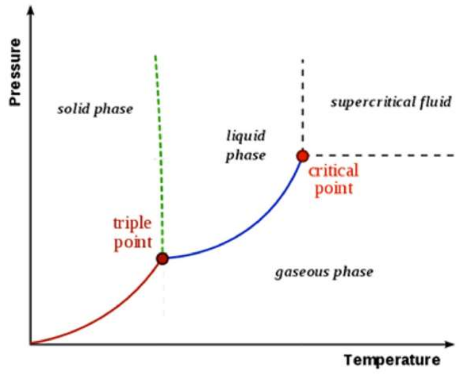
Supercritical steam, which is a special state of water, is a relatively new working fluid in industry that forms part of this research. As can be seen in Figure 1, the critical point of a fluid marks the terminus of the vapor–liquid coexistence curve. At temperatures above the critical temperature, a fluid cannot undergo a transition to a liquid phase, regardless of the pressure applied. A fluid is “supercritical” when its temperature and pressure exceed the temperature and pressure at the critical point [22].
Supercritical fluids possess properties that make them attractive as media for chemical reactions. It may be advantageous for reactions involved in fuel processing, biomass conversion, biocatalysts, homogeneous and heterogeneous catalysis, environmental control, polymerization, materials synthesis, and chemical synthesis [22].
Supercritical steam cycle in particular, creates an improved Rankine cycle at supercritical pressure and temperature, aiming at higher thermodynamic cycle efficiency, and thus, lower power generation costs. Coal fired power plants exist using such supercritical steam cycle since the 1990s [23]. Recently, more advanced coal-fired over-supercritical (OSC) and ultra-supercritical (USC) steam power plants reached the efficiency of 47% [24]. In nuclear power plants, water-cooled nuclear reactors operating at subcritical pressures (7–16 MPa) have provided significant electricity production for the past 50 years. However, the thermal efficiency of current nuclear power plants is between 30–35%. Hence, more competitive designs with higher thermal efficiencies, around 45 to 50%, need to be developed and implemented [25]. Recent design studies of a supercritical steam cycle for nuclear power plants, aiming at higher thermal efficiencies and heat flux, are ongoing. Such reactors have never been built up to now [23]. The fourth generation FBNR nuclear reactor design is considering the use of supercritical steam as its coolant [26].
2. Materials and Methods
In this work, the pressure drops of water fluid flowing in a fixed bed of spheres, set in different structure formations, are studied using the SolidWorks code. The fluids were water at 20 °C at 160 bar, 300 °C at 160 bar, and critical steam of 400 °C at 220 bar pressure. The structures chosen were faced-center cubic (FCC), body-centered cubic (BCC), and random structures. The methodology used to gain thermodynamics properties, CFD code, and turbulence modeling are presented as follows.
2.1. New Data Obtained from HYSYS
The water properties available in SolidWorks engineering database are limited to 200 °C. Therefore, HYSYS code and “ASTM steam” fluid package were used to generate data in an extended range needed for these calculations, including 300 °C and 400 °C conditions.
To define any state of saturated liquid, one only needs one other property, such as temperature or pressure. Therefore, all properties have been developed for 1 to 370 °C by 1 °C step intervals. But in the case of supercritical steam, two independent properties are needed. Then, the pressure of 220 bar was fixed, and all properties have been developed for temperatures from 374 to 600 °C by 1 °C step size. Just to illustrate, the curves obtained from HYSYS, density, and mass enthalpy are shown in Figure 2.
All of the required data is obtained from HYSYS and then transferred into the “User-defined” liquid in material section of SolidWorks Engineering Database. They have been utilized for hot water (300 °C) and supercritical steam (400 °C) coolant cases.
2.2. SolidWorks Code
SolidWorks is a solid modeling computer-aided design (CAD) and computer-aided engineering (CAE) computer program, published by Dassault Systèmes. SolidWorks Flow Simulation is a user-friendly and robust add-in of SolidWorks, which utilizes FV method on a rectangular (parallelepiped) computational mesh to solve time-dependent Navier–Stokes equations, and has been used in this study as a CFD tool. This method is among the preferred methods for fluid phenomena modeling.
2.3. Turbulence Modeling
Turbulence modeling, along with grid generation and algorithm development, is one of three key elements in CFD. Turbulence is inherently three dimensional and time dependent, but usually something less than a complete time history over all spatial coordinates for every flow property is needed. Since turbulence consists of random fluctuations of the various flow properties, a statistical approach should be used. Reynolds in 1895 introduced a procedure in which all quantities are expressed as the sum of mean and fluctuation parts [27]. In turbulent flow, the velocity is divided into two parts: one time-averaged part , which is independent of time (when the mean flow is steady), and one fluctuating part , so that [28].
Turbulent flow is irregular and chaotic, but it still is governed by Navier–Stokes equation. The flow consists of a spectrum of different scales known as eddy sizes. These turbulent eddies have no exact definition, but they are supposed to exist in a certain region in space for a certain time. Their energy is cascading from largest eddy to smallest eddy, and finally, the rotational kinetic energy of them is dissipated through friction or viscous forces.
Two fundamental equations, continuity equation and Navier–Stokes equation for incompressible flow, are used to define the problem. By dividing the velocity term in mean and fluctuating part, these equations become
The new term () is called Reynolds stress tensor, which is defined as an additional stress term due to turbulence, and it is unknown. Modeling this term is necessary to close the Navier–Stokes equation; this is called the closure problem. Algebraic models, one-equation models, two-equation models, and Reynolds stress models are different types of turbulence models, defined to address the closure problem, which have been listed in increasing order or complexity [9]. The detailed presentation and discussion of these turbulence models are referred to Wilcox [27].
First, the two abovementioned modeling methods are incomplete, which means certain knowledge about the studied flow in advance is needed. However, the first complete model was introduced by Kolmogorov in 1942, which modeled the turbulence kinetic energy (k) and the rate of energy dissipation (ω). Since two additional equations are considered in k–ω modeling, it is called the two-equation model. The k–ε model is a variation of this concept, in which turbulent dissipation (ε) is modelled instead of ω. Reynolds stress models (RSM), on the other hand, is the most physically sound model solving the problem directly using transport equations, avoiding the isotropic viscosity assumption of other models [29]. This method, which is usually used for highly swirling flows like cyclones, utilizes seven additional equations to model the turbulence which clearly increases the time and cost of the calculation to a great amount, which is also more difficult to converge.
SolidWorks does not cover a wide range of turbulence models, there are just two models, intensity–length (I–L) model which is a zero-equation model, and a two-equation model (k–ε). Since k–ε model is among the preferred turbulence models and the most common one, it has been chosen for calculation in this study.
In SolidWorks Flow Simulation, the k–ε model is used with a range of additional empirical enhancements added to cover a wide range of industrial turbulent flow scenarios (such as shear flows and rotational flows). For instance, damping functions proposed by Lam and Bremhorst (1981) for better boundary layer profile fit when resolving boundary layers with computational meshes have been added (the LB k–ε model). Therefore, it is a modified k–ε model with a unique two-scale wall function approach and immersed boundary Cartesian meshes. The detailed presentation and discussion of these modifications on k–ε model are available in a technical paper [30].
3. Results and Discussion
3.1. Modeling
3.1.1. Types of Bed Formations
The pressure drop of fluid flowing in a fixed bed depends on the porosity of the bed. The porosity depends on the structural formation of the bed by the manner that the particles are positioned, such as occurring in crystal formation. From a wide range of possible crystal structures, two of the most common ones are body-centered cubic (BCC) and face-centered cubic (FCC), that are chosen for this study. The third and the most realistic model is random distribution, which has been prepared by a SolidWorks motion study.
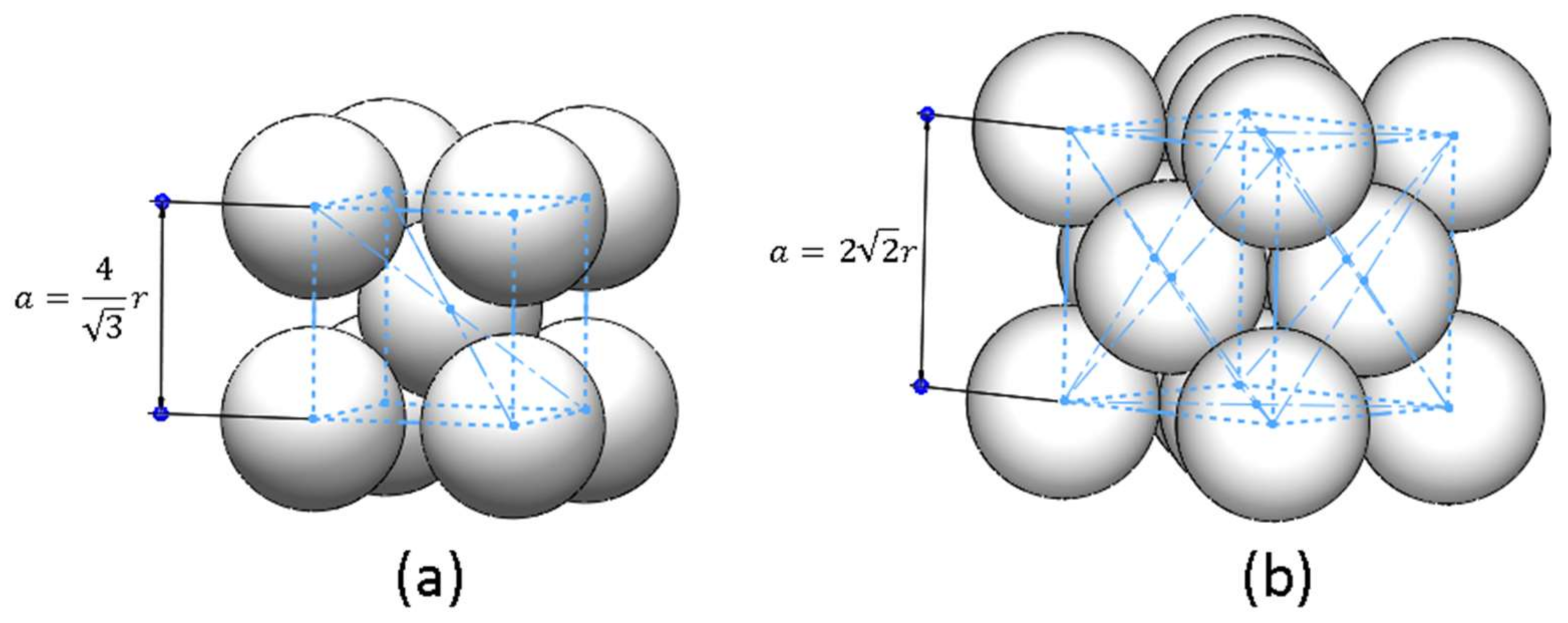
SolidWorks does not have pre-made models of unit cells of crystal structures, so they need to be built manually from scratch. The edge length of unit cells, as shown in Figure 3, for BCC and FCC, are well-established in many sources which are (4/√3 × r) and (2√2r), respectively. Using 3D sketch tool in SolidWorks, a cube with calculated edge length was drawn, and the required number of spheres were put into their places with the aid of Mate tool. To create larger models, these unit cells need to be duplicated with the aim of linear pattern along x, y, or z axis.
Establishing a way to create a random model, however, is followed by a completely different procedure. First, it is essential to estimate an approximate number of spheres which could fit into the tube with certain size; this usually starts with knowing the total volume of the bed, the probable porosity, and the volume of one sphere. Reported porosity of a random bed created by different codes are available in literature, and it has a value of roughly 0.4 [31]. After estimating the number of spheres and creating them with linear pattern, “motion study” feature is used to create the final model. The bed structure, as shown in Figure 4, is obtained in a simulation in which spheres fall down into a cylindrical container with the aid of gravity. In order to reach mechanical equilibrium, a funnel is used to slow down the spheres and save time until equilibrium is reached.
3.1.2. Investigation of Appropriate Model Dimensions
The key to a valid simulation is to create a model which is small enough to reduce calculation time, but at the same time, large enough to resemble reality. For FCC and BCC models, different numbers of unit cells are created to see which model would meet both abovementioned criteria. These models are illustrated in Figure 5 for FCC samples, and Figure 6 for BCC samples. The top line of both figures shows uncut models, and the bottom line shows cut models. The cut model refers to the situation where the spheres touching the wall are cut to become hemispheres, thus reducing and correcting the bed porosity at the wall.
The purpose of creating these samples is to determine how the pressure drop is going to change with increasing the size of the model or cutting the edges. Around 2,000,000 cells (meshes or control volumes) are used for pressure drop calculation of each sample, which is the maximum allowable number of cells with the available computer capacity. The results are shown in Table 1.
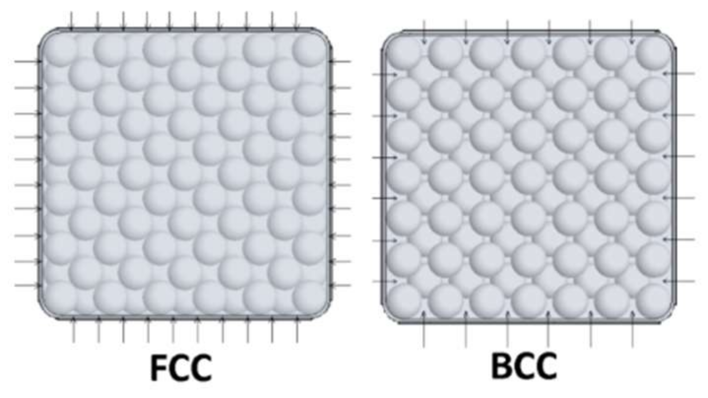
As can be seen, in both BCC and FCC structures, pressure drop varies dramatically from uncut to cut models. This is due to the effect of increased void at the wall, which affects the porosity, consequently affecting the pressure drop. Arrows in Figure 7 demonstrate some empty spaces which let the fluid flow freely. Therefore, it is more adequate to use cut models for pressure drop calculations that are closer to reality.
Pressure drop values for all cut models are relatively close to each other, but on the contrary with expectations, the larger model was chosen in order to create the correct porosity for a random model with same model dimensions. At very low tube to particle diameter ratios, the porosity of the random model would not be well-established. Therefore, a 10 × 10 × 20 cm model is used for all the calculations which is close to 4 cut model dimensions.
3.1.3. Mesh Study and Its Optimization
SolidWorks Flow Simulation 2017 has seven levels of initial mesh. The higher the number, the more times a cell’s size has been reduced, and thus, the finer the mesh. If more accurate results are needed, there is a refinement option which allows one to reduce the mesh size even more.
The refinement level is the maximum number of times a cube that represents a cell can be split. As shown in the Figure 8, each cube splitting into 8 equal cubes represents one level [32].
Adaptive mesh refinement, a facility to adapt the computational mesh to the requirements of the flow field by identifying of regions containing important features, helps the refinement process to be more time efficient by refining only necessary cells [33,34].
A method to evaluate the effect of these mesh sizes on the accuracy of the calculation needed to be established. Volume of spheres is one parameter where its value can be known beforehand and compared with the obtained result after meshing. If the meshes are not dense enough, the reported volume of spheres would not be the same as its actual values. This has a direct effect on porosity, which is a crucial parameter in pressure drop calculation, so one needs to make sure this value is as close to reality as possible. Mesh density also has an influence on the fluid cells and how properly their properties are calculated. The ratio of calculated volume of spheres to its real volume is shown in Table 2 for different mesh levels.
SolidWorks Flow Simulation has the ability to adapt the computational mesh to the solution during the calculation. The software splits the mesh cells in the high-gradient flow regions, and merges the cells in the low-gradient flow regions. This ensures better accuracy during the calculation. The mesh starts from an initial state and is modified during the calculation based on user-defined settings.
The refinement level specifies how many times the initial mesh cells can be split to achieve the solution-adaptive refinement criteria. For example, if the refinement level is set to three, and there are two-level initial mesh cells, the solution adaptive refinement process can split these cells down to five-level cells. So 7RL1 (seven-level initial mesh cells and one refinement level) is basically an initial mesh level of 8. The difference is that this refinement is applied after seven-level initial mesh convergence so that it is more time efficient.
Table 2 and Figure 9a illustrate initial meshes lower than three are too low, and cannot be used even if accuracy is not important. The error in volume calculation decreases gradually, reaching less than 2.5% at level 7 of initial mesh with one level of refinement (7RL1), and then levels off. Due to the fact that it is intended to obtain results at highest possible accuracy, further calculations are done with (7RL1) meshes. The second level of refinement (7RL2) has also been done for three bed formations, but the volume did not change effectively (not even 0.1%) while the calculation time surges to 60 h, which proves the impracticality of higher levels of refinement with present computer resources.
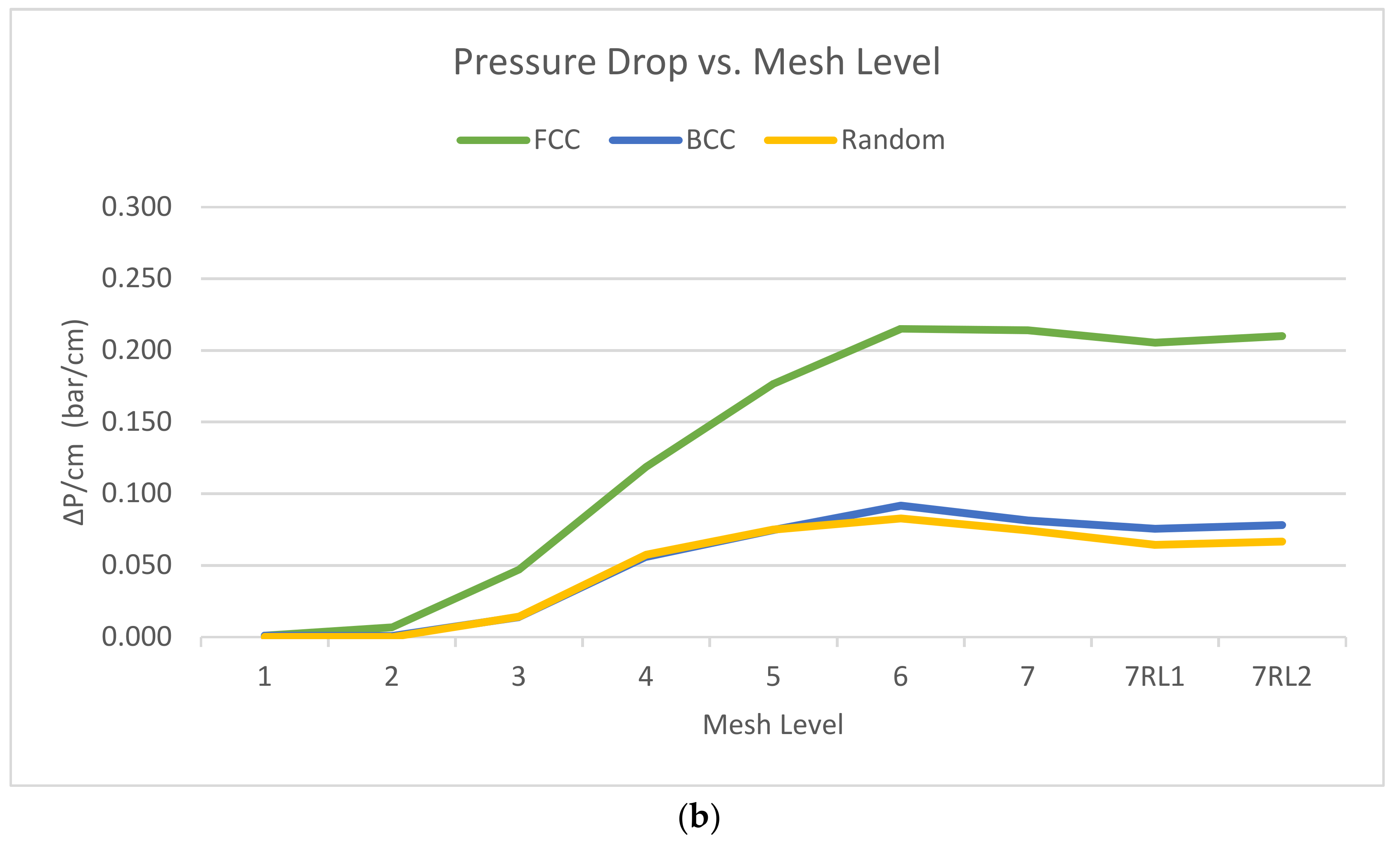
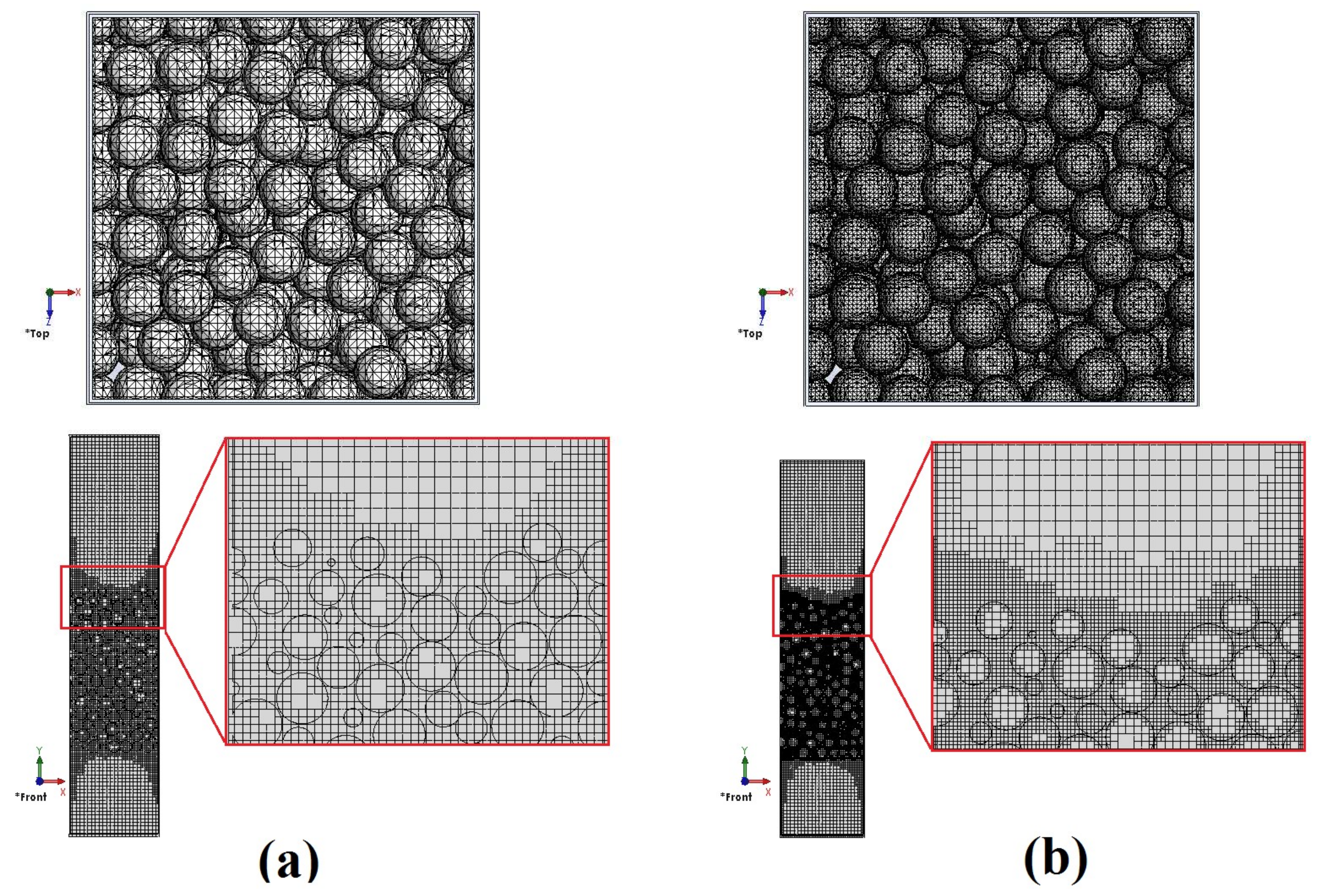
Pressure drop for each mesh level is plotted in Figure 9b. As one can see, the pressure drop values for mesh levels lower than 6 are not stabilized, but they remain almost unchanged between 7RL1 and 7RL2, which demonstrates 7RL1 is the optimized mesh level for calculations. The results of the mesh capturing for 7 and 7RL1 cases are shown in Figure 10 from both top view and cut section of front view.
From top view in Figure 10, it can be seen how decreasing mesh size improves the sphericity of the particles, which is essential for the calculation. Cut plot of front view also gives valuable information; one can see how adaptive mesh refinement identifies the important regions inside the bed, especially near the wall and inside the packing of spheres, and leaves unnecessary parts of the model with coarser meshes, helping to increase time efficiency of calculation process.
3.1.4. Study of Bed Porosity
Porosity or void fraction (ε) is a measure of the void spaces in a packing bed, which varies between 0 and 1. It could be easily measured by knowing the total volume of the bed and the space occupied by spheres. In crystal structure studies, atomic packing factor (APF) is a widely-used alternative which is convertible to porosity by the expression of “”. In a random model, unlike crystal structures, there is no solid geometry-based calculation for porosity, because the orientation of the spheres is highly dependent on how their contact is taken into account, and there is no repetitive pattern equivalent to unit cell concept in crystal structures. The porosity of models were calculated by the volumes given by SolidWorks, and compared with reported values in literature, as shown in Table 3. In order to make the porosity at the wall compatible with the bed porosity, the spheres touching the wall were cut into hemispheres. These cut models are shown in Figure 11. The numbers, rounded up to two digits, shows the 3D models prepared by SolidWorks have the same porosity as the reported ones in literature for crystal structure, and close enough to the random model.
3.2. Results
3.2.1. Pressure Drop in Different Fixed Bed Formation as a Function of Flow Velocity
Flow visualization is an important tool used to understand the physics of complex eddying motion and turbulence, giving qualitative and quantitative information [37,38,39]. Historically, experimental methods, such as smoke or dye injection, were developed to do visualization, but nowadays, with the aid of CFD method, purely computational methods are developed and used widely. Also, flow visualization in CFD becomes important as a way to display large amount of information yielded from numerical solution in a meaningful and visual form. First, with flow visualization technique, the water penetration in a fixed bed and its velocity distribution are visualized.
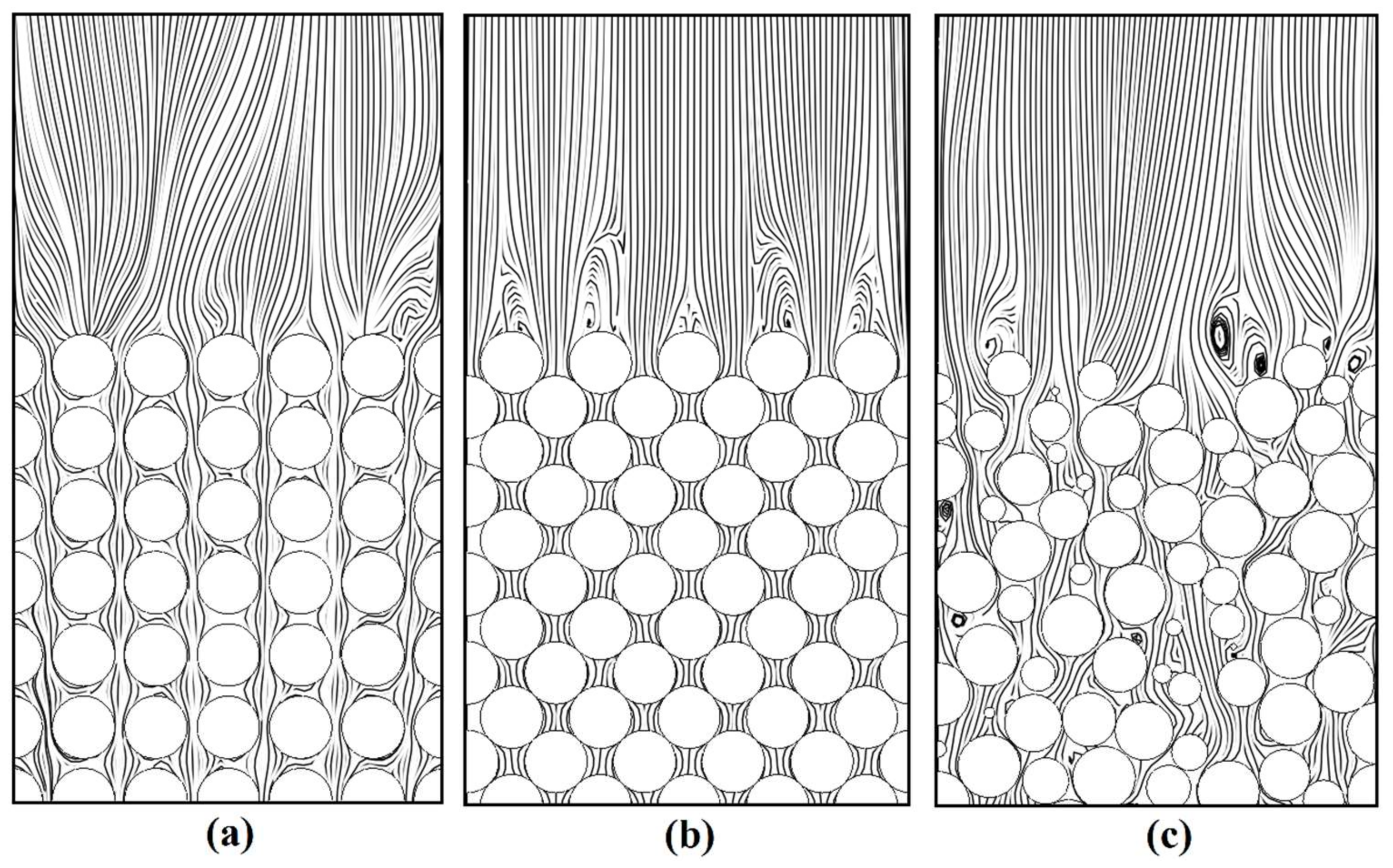
In Figure 12, streaklines of water at 20 °C and 160 bar pressure at 1 m/s velocity in three different bed structures are illustrated. It can be seen how the bed structure and void distribution affect the movement of the fluid between the spheres. In structured arrangements (BCC and FCC), a more repetitive pattern has been created, but in the third one (random and unstructured bed) streaklines are more chaotic, and also reverse currents and eddies are more common.
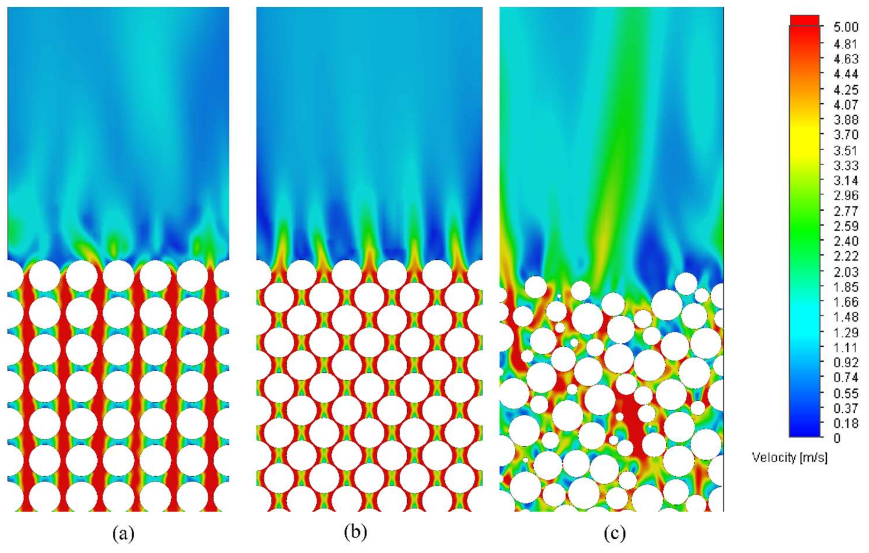
Velocity distribution is another important parameter that can be shown by CFD visualization technique. As one can see in Figure 13, the denser the bed is, the higher the velocity of fluid between the packing structures that can be expected. Increasing in the amount of velocity means the higher pressure drop does occur, but it has an advantage of better cooling and enhanced mixing when heat or mass transfer is involved.
To begin to find a relationship for pressure drop in fixed bed, generally, its dependency on fluid velocity (U) could be shown as Forchheimer law, described as , in which A and B are constants. Darcy’s law is an equation that describes the flow of a fluid through a porous medium which states a proportional relationship between the discharge rate through a porous medium, the viscosity and the pressure drop, only valid for creeping flows. Forchheimer observed that as the flow velocity increases, the inertial effects start dominating the flow. In order to account for these high velocity inertial effects, he suggested the inclusion of an inertial term representing the kinetic energy of the fluid to the Darcy equation [40]. This term is able to account for the non-linear behavior of the pressure difference vs flow data. In this study, the Forchheimer law is applied to investigate how this general equation works for higher velocities and Reynolds numbers.
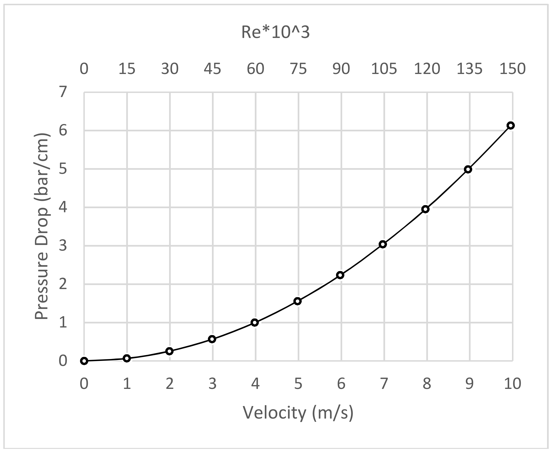
Water at 20 °C flowing through the random packing of 15 mm spheres is studied. SolidWorks permits velocity and pressure at entrance and exit of the sample for internal fluid cases. One can only choose one parameter for a boundary. In this study, various velocities added in the entrance of the sample and fixed pressure of 160 bar are applied on exit of the model as boundary conditions. Certain goals, the terms used by SolidWorks for parameters, such as entering and exit pressure and density, are also defined to monitor important parameters inside the bed for calculation.
The results were plotted as shown in Figure 14. After curve fitting, it was found that the data perfectly matches with Forchheimer law with R2 (coefficient of determination) of 1, and the equation is . Since the fitted curve follows the general expected equation, this attempt shows promising results.
3.2.2. Pressure Drop in Different Fixed Bed Formation as a Function of Particle Size
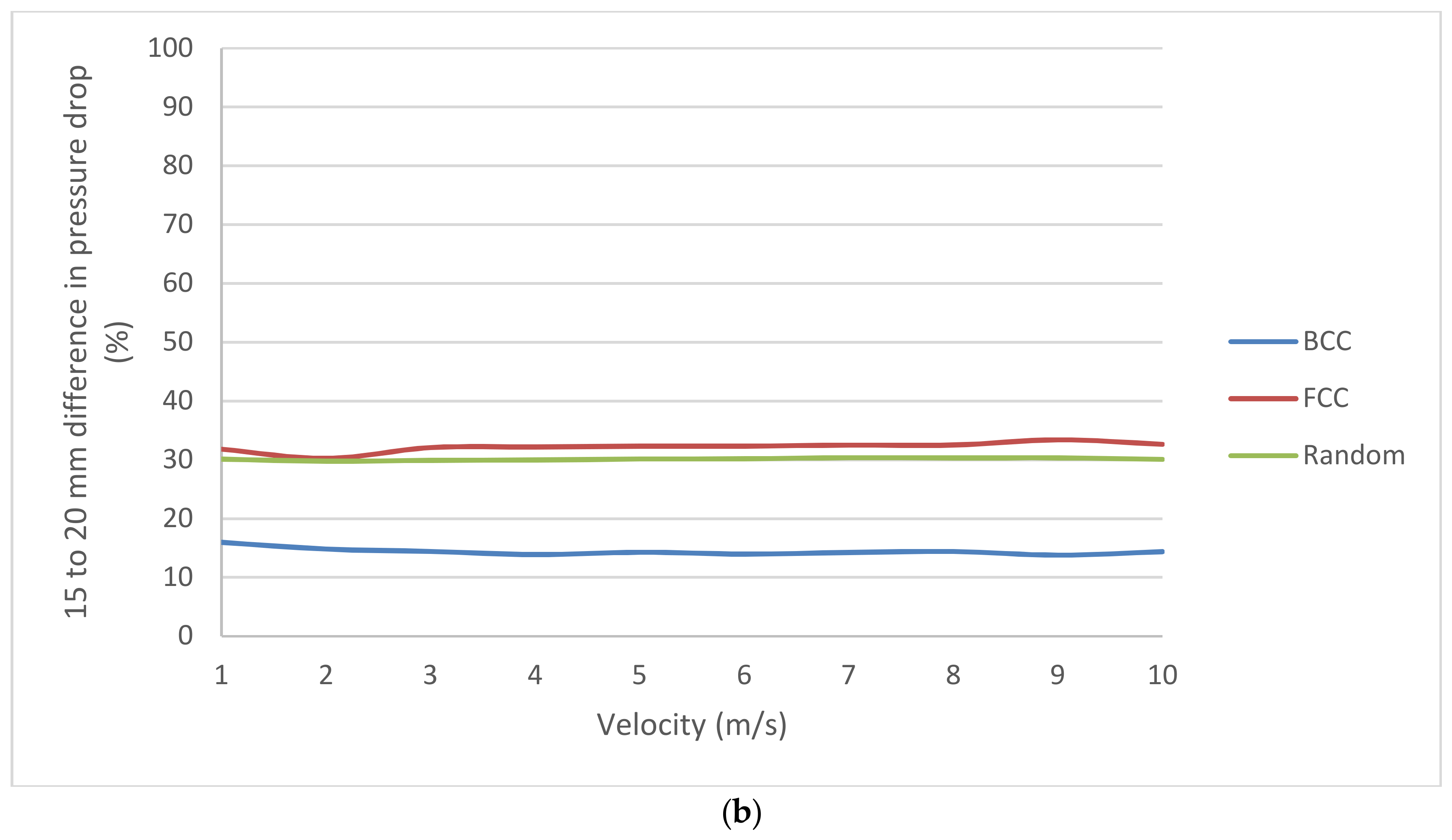
Particle diameter is an important characteristic of the bed, but it does not affect porosity. Calculations are made also for 20 mm spheres, while all other parameters remain constant. This process has been done for all three fixed-bed structures, namely FCC, BCC, and random, and shown in Figure 15a.
Pressure drop is inversely proportional to particle diameter. The percentage differences in pressure drop as a function of flow velocity for different bed structures are shown in Figure 15b. The average is about 14.4% for BCC, 32.2% for FCC, and 30.1% for random model. Since the increase in particle diameter was 33.3%, in FCC and random cases, the pressure drop seems to be inversely proportional to the particle diameter.
The study shows that pressure drop values are close to each other in BCC and random model, while their porosities differ noticeably. Also, the average difference in pressure drop in BCC is much smaller than in FCC and random. These may be explained by the special pattern of BCC, which results in additional empty spaces between spheres, which let the fluid move freely through the bed, and consequently, have lower pressure drop than expectations.
3.2.3. Effect of Porosity on Pressure Drop
Porosity irrefutably has great importance in pressure drop calculations. The less the porosity is, the more difficult for the fluid to penetrate the bed, and as a result, the greater the pressure drop will be. As Ergun declared, fractional void volume has been one of the most controversial factors in packed systems. The effect of porosity is studied on previously mentioned prepared models with porosities of 0.32 for BCC, 0.26 for FCC, and 0.37 for random model. Water at 20 °C moves through the models, and its pressure drop is calculated for 1 to 10 m/s velocities, and the results are shown in Figure 16.
The first observation is that the difference in pressure drop of BCC and random model is lower than of BCC and FCC, despite the fact that their porosity values are so close (0.05 for random–BCC and 0.06 for BCC–FCC). Therefore, direct or inverse proportionality of porosity to pressure drop is refuted, and more complicated relationships have to be found. As shown in Equation (1), Ergun suggested the expression of for the part that viscous forces are dominant, and when inertial forces are. In KTA, as shown in Equation (4), these terms are and , respectively. Therefore, the general expression of , where n is constant, is suggested for including porosity in pressure drop equation.
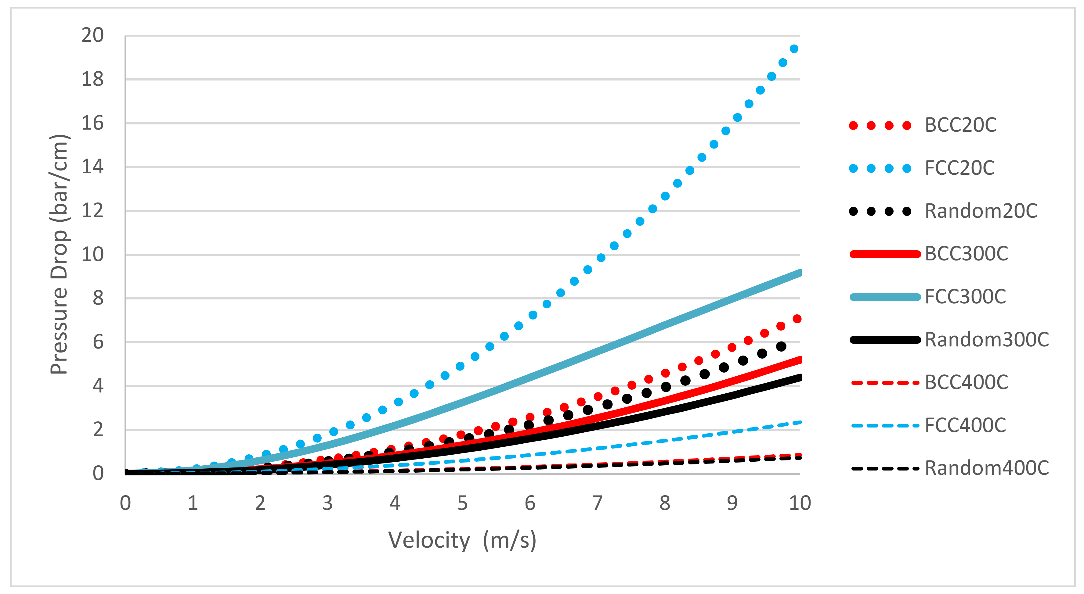
3.2.4. Effect of Water Density and Viscosity on Pressure Drop
The effect of density and viscosity is studied using water at three chosen temperatures. The required thermodynamic properties for flow simulation are presented in Table 4.
The graphs, shown in Figure 17, illustrate the effect of fluid density on pressure drop through a fixed bed. It can be seen that pressure drop is directly proportional to density. In Table 6, the ratio of pressure drops and their relative densities and viscosities are shown.
This shows that the pressure drop ratio is almost directly proportional to the density ratio with a slight difference, but the viscosity ratios did not show any meaningful relation with pressure drop. The fact that the viscous forces are not as effective as inertial forces at this high Reynolds number could be an explanation for this behavior. Since pressure drop is the sum of these two parts, the value of inertial forces are considerably higher than the viscous forces, and the final summation would be closer to the inertial forces part.
To investigate this hypothesis, the two parts of Ergun’s equation are calculated separately. Ergun correlation consists of two different parts, viscous and inertial, as shown with constants of 150 and 1.75 in Equation (1), respectively, which fits the pressure drop data for beds of spheres extremely well at low Reynolds number. To illustrate how the effect of these parts changes with respect to velocity, they have been calculated separately for water at 20 °C, 300 °C, and 400 °C, and the percentage of each part is plotted against velocities, ranging from 0.0001 to 10 m/s in Figure 18.
The viscous part becomes zero after 1 m/s in all cases, which confirm the validity of the explanation. Therefore, the viscous part in 1 to 10 m/s intervals in the case of water fluid can be eliminated, and the Ergun equation can be reduced to
In a similar manner, two parts of KTA formula, which also represent viscous and inertial forces, showed the same result; the first part with the coefficient of 160, representing viscous forces, is negligible at high velocities, and the second part with the coefficient of 3 is the dominant part of the equation at high velocities, which indicates inertial forces. Therefore, KTA formula can be reduced to
It could be concluded that pressure drop at such high velocities of water at any given temperature is highly dependent on density, but not significantly affected by viscosity.
The reduced forms of Ergun and KTA equations are similar to each other in many ways, 1/d, are exactly the same, is the same too, but n is slightly changed from 1 to 1.1, but the main difference is existence of Re number in KTA method, which has not been considered in Ergun’s equation, and also, the constants, which are 3 and 1.75 in KTA and Ergun equation, respectively. In Figure 19, the calculated pressure drop using Ergun, KTA, and SolidWorks CFD for water at three different temperatures in a random fixed bed of 15 mm spheres has been shown.
As one can see in Figure 19, Ergun highly overestimates the pressure drop, but the KTA is significantly close to CFD results, especially in the 300 °C and 400 °C cases.
3.2.5. Validation Test
Since experimental data for pressure drop with flow conditions similar to the calculated cases in our work are not available, in order to check the reliability of the approach, a single case where data was available has been tested. The required experimental data was obtained from a dissertation, by A.J.K. Van Der Walt [41], in which pressure drop through three different fixed bed of random spheres was measured in the High Pressure Test Unit (HPTU).
HPTU was designed, built, and successfully commissioned to provide a facility capable of producing the range of experimental results required. There was, thus, three different homogeneous porosity test sections for the pressure drop test. They were referred to as PDTS 036 for the 0.36 porosity test section, and likewise, for the 0.39 and 0.45 porosities, the tests were labelled PDTS 039 and PDTS 045, respectively. PDTS cases were random fixed bed, with reported dimensions in Table 7, composed of translucent acrylic spheres with diameter of 1.125 inch, or 28.575 mm. The working fluid for all the tests was high purity nitrogen, capable of producing particle Reynolds numbers from 1000 up to 50,000, by varying the system pressure, from 1 to 50 bars, at a constant volume flow rate.
Instead of direct value for pressure drops, the friction factor has been provided, which is related to pressure drop by the below relation:
in which is pressure drop, is fluid density, is superficial average velocity, is particle diameter, L is length of the bed, and is average porosity.
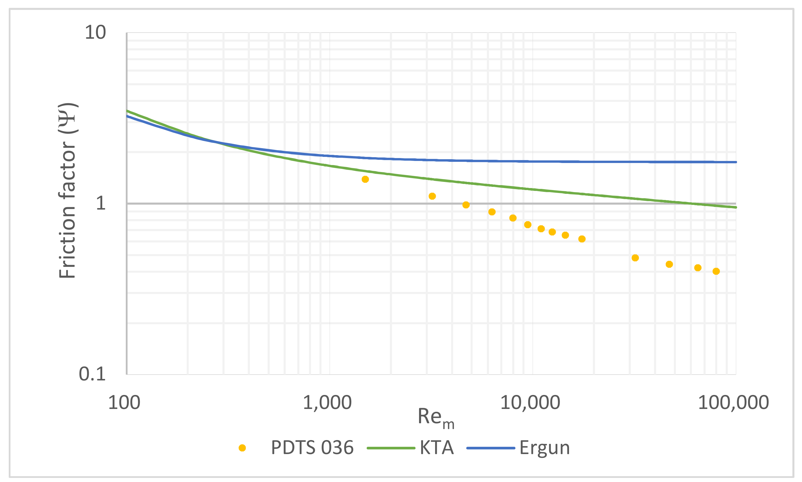
As one can see in Figure 20, a comparison of experimental data of PDTS 036 [41] with KTA and Ergun correlations has been provided, in which friction factors is plotted against modified Reynolds number with definition of
Percentage differences between KTA prediction and experimental friction factors for homogeneous porosity test sections are also presented in Table 8.
The validation test has been done for the case of Reynolds number of approximately 10,000 for the 0.36 porosity test section (PDTS 036). As can be seen in Figure 20, friction factor values for this case are 1.75, 1.22, and 0.75 for Ergun, KTA, and PDTS 036, respectively.
To simulate this case, a random model, composed of around 800 spheres, is designed in SolidWorks, and pure nitrogen, at a pressure of 10 bars with density of 11.45 kg/m3, was passed through the bed with the velocity of 0.3356 m/s, resulting in modified Reynolds number of 9450. Mesh level of 7RL1 was also defined for the bed, and the calculated pressure drop for 40 cm of bed became 187 pa, which is equivalent of friction factor of 0.755, as shown below:
The calculated friction factor by SolidWorks simulation (0.755) is within acceptable agreement with the experimental data (0.75) so it can be concluded the approach used in this work is reliable.
In another study, by Preller [1], a computational approach was used. Nitrogen at 26.85 °C, as an ideal gas, with uniform inlet velocity of 0.4487 m/s was passed through a random fixed bed created in SolidWorks 2010. The pressure on the outlet was 101.325 kPa, resulting in a modified Reynolds number of approximately 1200.
As shown in Table 9, the pressure drop results obtained from simulations, using STAR-CCM+ (VERSION 6.02.011) as a CFD tool, as well as the deviation when compared with the theoretical pressure drop for each of the mesh independency (MD) tests, have been reported.
3.2.6. New Equation for Pressure Drop in Fixed Bed
Observations from previous sections suggest the new equation to be in the form
in which is the pressure drop in Pa, L is the height of the bed in m, is the bed porosity, is the particle diameter in m, is fluid density in kg/m3, is superficial velocity, represents particle Reynolds number, and finally, and are constants.
Excel Solver has been used to calculate these constants, which fit all of the SolidWorks data in the best possible way. To examine the closeness of equations to data, the term for all data has been calculated. The square root of the summation of this term, divided by the number of cases, shows how much the average error is. A lower value is better and shows less deviation. First, KTA constants which are 3, 0.1, and 1.1 are put into the equation, and the average error becomes 1.6. Then, Excel Solver is used to minimize the average error by changing the constants, resulting in 0.46 value with average error 3.26, 0.13, 1.26 for a, b and n, respectively. Therefore, we offer using the below equation for pressure drop calculation in fixed bed in high particle Reynolds number condition between 15,000 and 1,000,000 for porosities between 0.26 and 0.37:
Because poured random packing is the most widely used form of fixed bed in industry, and its porosity is limited to values close to 0.37, the same process has been done only on data obtained from a random model to achieve a more accurate equation. This made an extraordinarily perfect fitting with the average error of 0.064, which means the below formula perfectly coordinates with the SolidWorks data, and we encourage using this equation when more accurate pressure drop is needed for random close packing of spheres:
It has to be mentioned that this equation is capable of predicting pressure drops in random bed formation (porosity of 0.37 or possibly near values to that). Just to show how accurate the above equation for random packing is, the SolidWorks data (SW) and the estimated pressure drop (NewEqu.) against fluid velocity at 20 °C, 300 °C, and 400 °C are plotted in Figure 21.
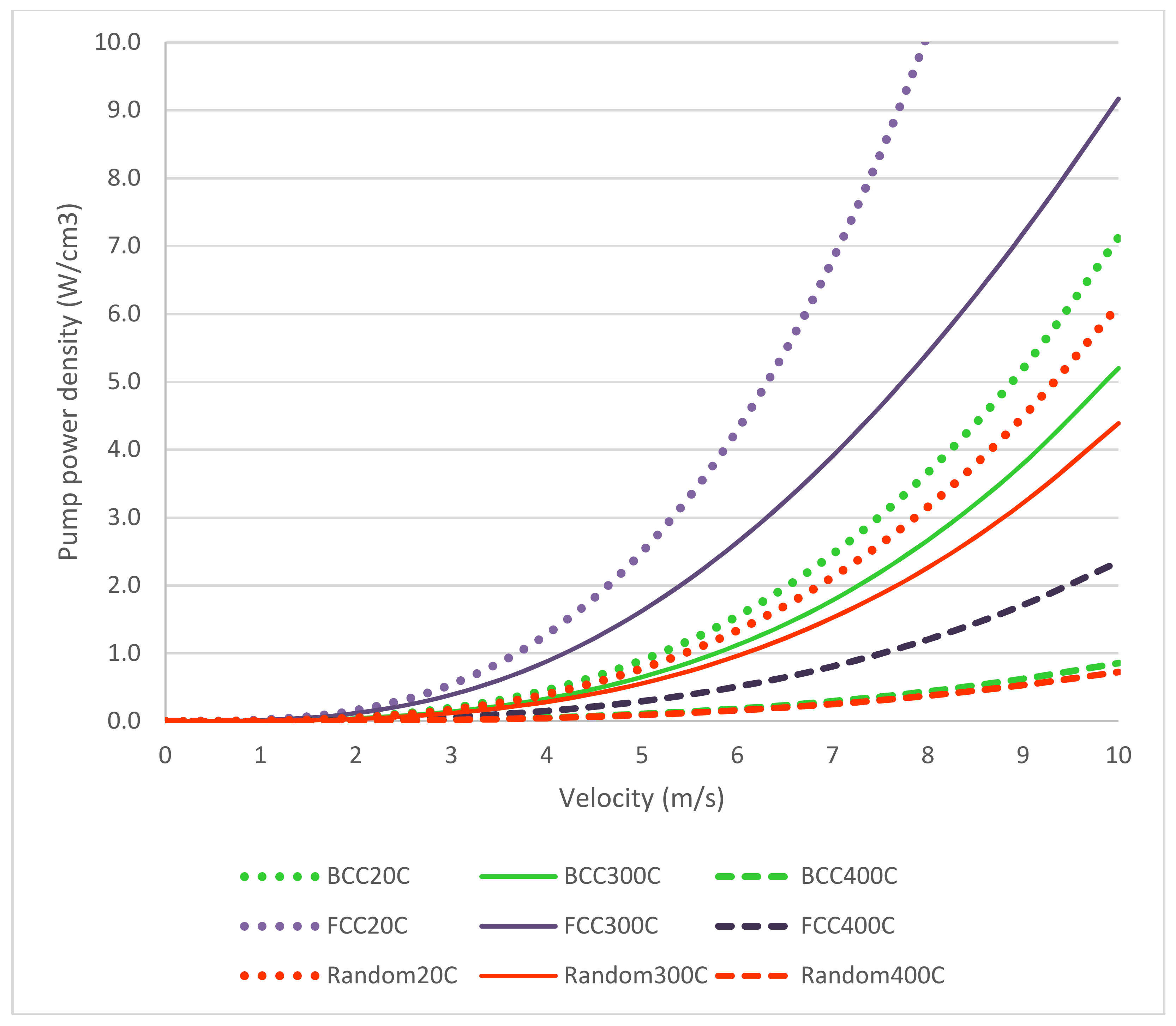
3.2.7. Required Pump Power
Power is consumed by a pump in order to increase the pressure of a fluid to penetrate the fixed bed. The power requirement of the pump depends on a number of factors, including the differential pressure, the fluid density, viscosity, and flow rate. The hydraulic power which represents the energy imparted on the fluid being pumped to increase its velocity and pressure. It is calculated by the following Equation (14):
where PP in W/cm3, ∆P in bar/cm, V in m/s, and 0.1 coefficient is for unit conversion. Details on the derivation of Equation (14) are given in Appendix A.
Pressure drop, occurring as a result of resistance to flow in fixed bed, is represented in Figure 22. The pump power is reported as pump power density form, with units of W/cm3. This represent the amount of energy needed to penetrate 1 cm2 surface of fixed bed for 1 cm height of the bed.
4. Conclusions
Fixed beds are used extensively in different industries. The parameter which is of most importance in engineering design of fixed beds is the pressure drop of fluid flow caused by the presence of the media. From a fluid mechanics point of view, it is essential to know the behavior of the fluid inside the bed to understand the characterization of fixed beds. Traditional experimental methods are time- and money-consuming, with technical difficulty of measuring flow parameters inside the fixed beds. Therefore, computational fluid dynamics (CFD), which solves flow and energy balances in complicated geometries, numerically, is the best alternative available.
In this work, a comprehensive study of pressure drop in fixed bed has been performed. SolidWorks code 2017 is utilized to create adequate models with dimensions of approximately 10 × 10 × 20 cm in three BCC, FCC, and random orientation of spheres in the fixed bed. Then, SolidWorks Flow Simulation, a robust SolidWorks add-in, is used as CFD tool. About 2,000,000 cells are generated with adaptive mesh refinement technique, certain boundary conditions are applied, and the results of calculation are collected for analysis.
The obtained results are compared with two well-known pressure drop correlations in the literature, namely Ergun and KTA. The case of interest of relatively high velocities of water flow, and consequently high Reynolds numbers, were studied. Ergun’s equation was not compatible with the calculated pressure drops in this work; KTA equation performed considerably better, but still did not achieve the best possible fitting. Consequently, using Excel Solver, the best fitting for the SolidWorks results were achieved and presented. Required pump power to overcome the pressure drop is also calculated for engineering design purposes.
Pressure drops of water and critical steam flowing in the fixed bed of mono-sized spheres are studied using SolidWorks Flow Simulation CFD code. Due to the limitation of computer resources, small models were needed to be designed to represent the whole reactor system. Wall effect, where the porosity at the wall is higher than the average bed porosity, is needed to be eliminated. Therefore, the spheres touching the wall were cut into hemispheres. It is verified that by this, the porosities, obtained from the results of SolidWorks calculations, correspond to published values in literature [35,36]. The trend shows that the pressure drops, also, in such models would be almost the same as in larger systems.
One of the most important criteria in measuring the accuracy of mesh density is by means of a mesh independency study, which is seldom shown in most CFD studies found in literature. Even though the code suggests mesh level of 3 in this study, mesh level of 7 with one more additional level of refinement was found to be satisfactory.
The effects of the type of bed formation, flow velocity, density, and pebble size are evaluated. The study of random, BCC, and FCC fixed-bed formations show that pressure drop increases in this order. FCC, having the densest packing, has the lowest porosity among other formations. Therefore, studying a reactor assuming FCC formation will result in indicating the extreme case with dramatic pressure drop variation compared to the two other formations. For practical purposes, pressure drop values are almost the same in random and BCC models, while their porosities differ noticeably. This unexpected behavior of BCC may be explained by it special pattern, which results in empty spaces between spheres, and lets the fluid move freely through the bed, and consequently, experiences a lower pressure drop than expected.
In the next part, the SolidWorks results have been compared with two well-known pressure drop calculation equations, namely Ergun and KTA. An equation, similar to that of KTA, is proposed to evaluate the pressure drop of water and critical steam in a fixed bed at high Reynolds numbers, applicable for particle Reynolds numbers ranging from 15,000 to 1,000,000.
The pump power (W/cm3) necessary to compensate the pressure loss are also evaluated in fixed beds of different formations.
Acknowledgments
The authors acknowledge the support from the Chemical Engineering Department of BIHE. The help received through consultations with Professor Sohrab Rohani and Professor Behzad Mottahed, the professors of the Baha’i Institute for Higher Education (BIHE), are also greatly appreciated.
Author Contributions
The project was conceived and supervised by Professor Farhang Sefidvash and the rest of the works were done by Soroush Ahmadi.
Conflicts of Interest
The authors declare no conflict of interest.
Appendix A
Details on the derivation of Equation (14) are given below:
0.1 coefficient is obtained from
References
- Preller, A.C.N. Numerical Modelling of Flow through Packed Beds of Uniform Spheres; North-West University: Potchefstroom, South Africa, 2011. [Google Scholar]
- Ahn, D.-H.; Chang, W.-S.; Yoon, T.-I. Dyestuff wastewater treatment using chemical oxidation, physical adsorption and fixed bed biofilm process. Process Biochem. 1999, 34, 429–439. [Google Scholar] [CrossRef]
- Hayashi, H.; Taniuchi, J.; Furuyashiki, N.; Sugiyama, S.; Hirano, S.; Shigemoto, N.; Nonaka, T. Efficient recovery of carbon dioxide from flue gases of coal-fired power plants by cyclic fixed-bed operations over K2CO3-on-carbon. Ind. Eng. Chem. Res. 1998, 37, 185–191. [Google Scholar] [CrossRef]
- Rycroft, C.H.; Grest, G.S.; Landry, J.W.; Bazant, M.Z. Analysis of granular flow in a pebble-bed nuclear reactor. Phys. Rev. E 2006, 74, 021306. [Google Scholar] [CrossRef] [PubMed]
- Şahin, S.; Sefidvash, F. The fixed bed nuclear reactor concept. Energy Convers. Manag. 2008, 49, 1902–1909. [Google Scholar] [CrossRef]
- Dossat, V.; Combes, D.; Marty, A. Continuous enzymatic transesterification of high oleic sunflower oil in a packed bed reactor: Influence of the glycerol production. Enzym. Microb. Technol. 1999, 25, 194–200. [Google Scholar] [CrossRef]
- McCabe, W.L.; Smith, J.C.; Harriott, P. Unit Operations of Chemical Engineering, 7th ed.; McGraw-Hill: Boston, MA, USA, 2005; p. xxv. 1140p. [Google Scholar]
- Baker, M.J. CFD Simulation of Flow through Packed Beds Using the Finite Volume Technique. Ph.D. Thesis, University of Exeter, Exeter, UK, 2011. [Google Scholar]
- Davidson, L. An Introduction to Turbulence Models; Chalmers University of Technology: Goteborg, Sweden, 2016. [Google Scholar]
- Ergun, S. Fluid flow through packed columns. Chem. Eng. Prog. 1952, 48, 89–94. [Google Scholar]
- Achenbach, E. Heat and flow characteristics of packed beds. Exp. Therm. Fluid Sci. 1995, 10, 17–27. [Google Scholar] [CrossRef]
- KTA. Reactor Core Design of High-Temperature Gas-Cooled Reactor. Part 3: Loss of Pressure through Friction in Pebble Bed Cores. Safety Standards, KTA 3102.3, Salzgitter, 1981. Available online: http://www.kta-gs.de/e/standards/3100/3102_3_engl_1981_03.pdf (accessed on 25 November 2017).
- Nijemeisland, M. Verification Studies of Computational Fluid Dynamics in Fixed Bed Heat Transfer; Worcester Polytechnic Institute: Worcester, MA, USA, 2000. [Google Scholar]
- Peiró, J.; Sherwin, S. Finite difference, finite element and finite volume methods for partial differential equations. In Handbook of Materials Modeling: Methods; Yip, S., Ed.; Springer: Dordrecht, The Netherlands, 2005; pp. 2415–2446. [Google Scholar]
- Miroliaei, A.R.; Shahraki, F.; Atashi, H. Computational fluid dynamics simulations of pressure drop and heat transfer in fixed bed reactor with spherical particles. Korean J. Chem. Eng. 2011, 28, 1474–1479. [Google Scholar] [CrossRef]
- Dalman, M.T.; Merkin, J.H.; McGreavy, C. Fluid flow and heat transfer past two spheres in a cylindrical tube. Comput. Fluids 1986, 14, 267–281. [Google Scholar] [CrossRef]
- Derkx, O.R.; Dixon, A.G. Determination of the fixed bed wall heat transfer coefficient using computational fluid dynamics. Numer. Heat Transf. Part A 1996, 29, 777–794. [Google Scholar] [CrossRef]
- Calis, H.P.A.; Nijenhuis, J.; Paikert, B.C.; Dautzenberg, F.M.; van den Bleek, C.M. CFD modelling and experimental validation of pressure drop and flow profile in a novel structured catalytic reactor packing. Chem. Eng. Sci. 2001, 56, 1713–1720. [Google Scholar] [CrossRef]
- Guardo, A.; Coussirat, M.; Larrayoz, M.A.; Recasens, F.; Egusquiza, E. CFD flow and heat transfer in nonregular packings for fixed bed equipment design. Ind. Eng. Chem. Res. 2004, 43, 7049–7056. [Google Scholar] [CrossRef]
- Gunjal, P.R.; Ranade, V.V.; Chaudhari, R.V. Computational study of a single-phase flow in packed beds of spheres. AIChE J. 2005, 51, 365–378. [Google Scholar] [CrossRef]
- Reddy, R.K.; Joshi, J.B. CFD modeling of pressure drop and drag coefficient in fixed and expanded beds. Chem. Eng. Res. Des. 2008, 86, 444–453. [Google Scholar] [CrossRef]
- Savage, P.E.; Gopalan, S.; Mizan, T.I.; Martino, C.J.; Brock, E.E. Reactions at supercritical conditions: Applications and fundamentals. AIChE J. 1995, 41, 1723–1778. [Google Scholar] [CrossRef]
- Lin, C.; Yuhiro, I. Advanced Applications of Supercritical Fluids in Energy Systems; IGI Global: Hershey, PA, USA, 2017; pp. 1–682. [Google Scholar]
- Tumanovskii, A.G.; Shvarts, A.L.; Somova, E.V.; Verbovetskii, E.K.; Avrutskii, G.D.; Ermakova, S.V.; Kalugin, R.N.; Lazarev, M.V. Review of the coal-fired, over-supercritical and ultra-supercritical steam power plants. Therm. Eng. 2017, 64, 83–96. [Google Scholar] [CrossRef]
- Naidin, M.; Pioro, I.; Mokry, S.; Grande, L.; Villamere, B.; Allison, L.; Rodriguez-Prado, A.; Mikhael, S.; Chophla, K.; Duffey, R. Super Critical Water-Cooled Nuclear Reactors (SCWRs) Thermodynamic Cycle Options and Thermal Aspects of Pressure-Channel Design; International Atomic Energy Agency (IAEA): Vienna, Austria, 2011. [Google Scholar]
- Schulenberg, T.; Leung, L. 8—Super-critical water-cooled reactors a2—Pioro, Igor L. In Handbook of Generation IV Nuclear Reactors; Woodhead Publishing: Sotheon, UK, 2016; pp. 189–220. [Google Scholar]
- Wilcox, D.C. Turbulence Modeling for CFD; DCW Industries, Inc.: La Cañada, CA, USA, 1993. [Google Scholar]
- Davidson, L. Fluid Mechanics. Turbulent Flow and Turbulence Modeling; Chalmers University of Technology: Goteborg, Sweden, 2017. [Google Scholar]
- Sodja, J. Turbulence Models in CFD; Faculty for Mathematics and Physics, Department of Physics, University of Ljubljana: Ljubljana, Slovenia, 2007. [Google Scholar]
- Enhanced Turbulence Modeling in Solidworks Flow Simulation. Available online: https://www.symsolutions.com/images/flow-white-paper.pdf (accessed on 9 October 2017).
- Roozbahani, M.M.; Huat, B.; Asadi, A. The effect of different random number distributions on the porosity of spherical particles. Adv. Powder Technol. 2013, 24, 26–35. [Google Scholar] [CrossRef]
- Meshing in Flow Simulation Part 3. Available online: http://blog.gxsc.com/graphics_systems_solidnot/2015/11/meshing-in-flow-simulation-part-3.html (accessed on 22 July 2017).
- Rose, T.; Smith, P.; Forth, S. Development of an Adaptive Mesh CFD Code for High Explosive Blast Simulation. In Proceedings of the 12th International Symposium on Interaction of the Effects of Munitions with Structures, New Orleans, LA, USA, 12–16 September 2005. [Google Scholar]
- Tautges, T.J. CGM: A geometry interface for mesh generation, analysis and other applications. Eng. Comput. 2001, 17, 299–314. [Google Scholar] [CrossRef]
- Campbell, F.C. Elements of Metallurgy and Engineering Alloys; ASM International: Materials Park, OH, USA, 2008; p. xiii. 656p. [Google Scholar]
- Scott, G.D.; Kilgour, D.M. The density of random close packing of spheres. J. Phys. D Appl. Phys. 1969, 2, 863. [Google Scholar] [CrossRef]
- Smits, A.J.; Lim, T.T. Flow Visualization: Techniques and Examples; Imperial College Press: River Edge, NJ, USA, 2000. [Google Scholar]
- Cantwell, B.J. Organized motion in turbulent flow. Annu. Rev. Fluid Mech. 1981, 13, 457–515. [Google Scholar] [CrossRef]
- Gharib, M.; Pereira, F.; Dabiri, D.; Modarress, D. Quantitative flow visualization. Ann. N. Y. Acad. Sci. 2002, 972, 1–9. [Google Scholar] [CrossRef] [PubMed]
- Jambhekar, V.A. Forchheimer Porous-Media Flow Models—Numerical Investigation and Comparison with Experimental Data; Universität Stuttgart, Institut für Wasser- und Umweltsystemmodellierung: Stuttgart, Germany, 2011. [Google Scholar]
- Van Der Walt, A.J.K. Pressure Drop through a Packed Bed; North-West University: Potchefstroom, South Africa, 2006. [Google Scholar]
Figure 1.
General phase diagram.

Figure 2.
Saturated water and critical steam HYSYS graphs (a) density; (b) enthalpy vs temp.
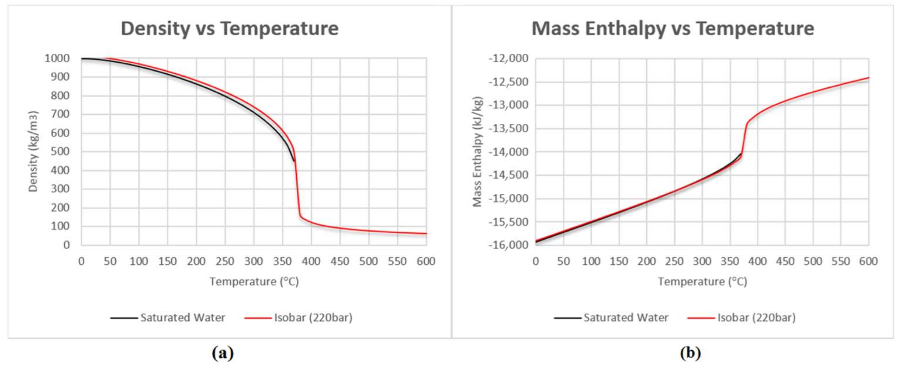
Figure 3.
(a) Body-centered cubic unit cell; (b) Face-centered cubic unit cell.

Figure 4.
Process of random model creation.
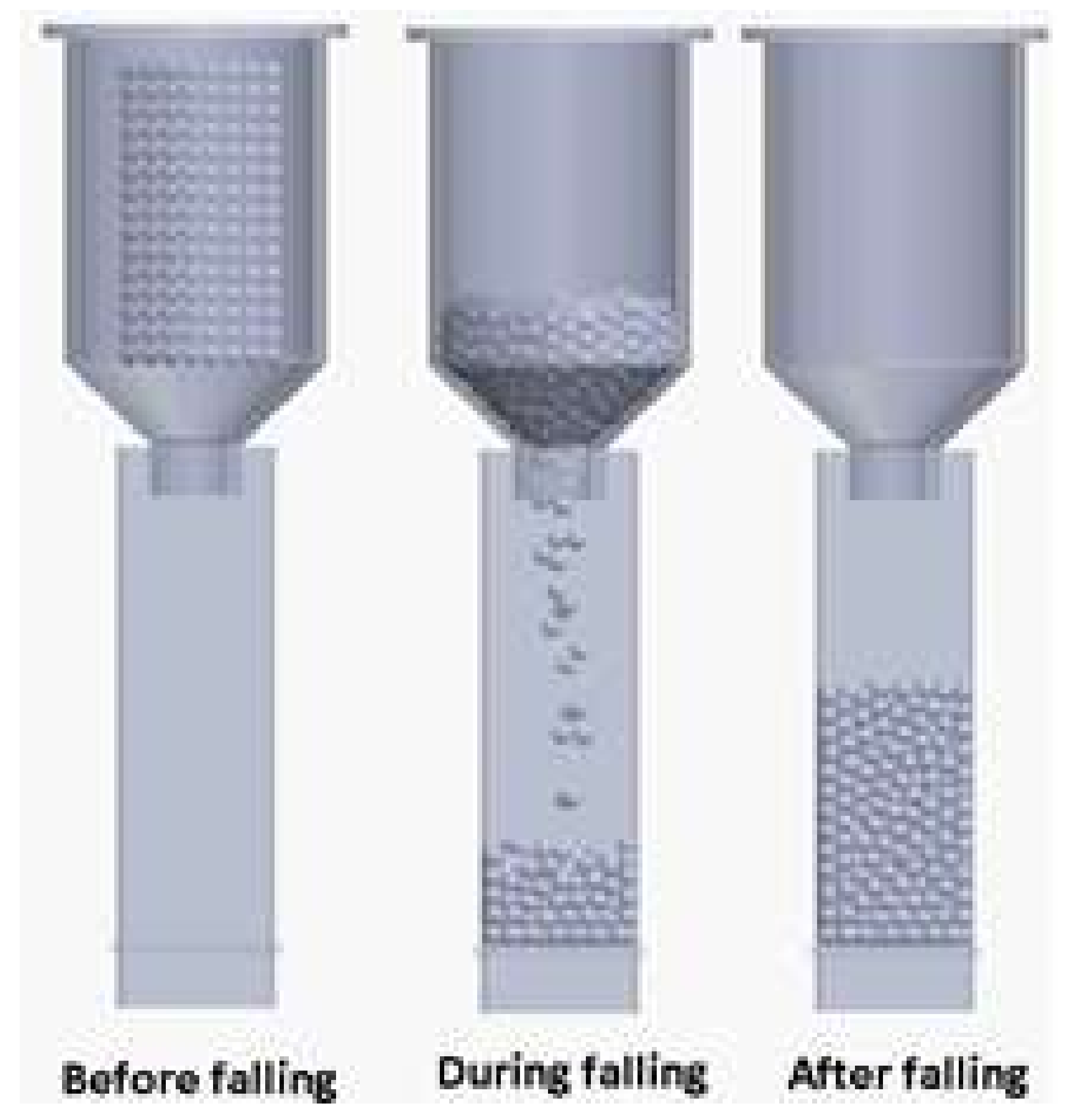
Figure 5.
Faced-center cubic (FCC) samples; named as (a) 1; (b) 2; (c) 3; (d) 4; (e) 1cut; (f) 2cut; (g) 3cut; (h) 4cut.
Figure 5.
Faced-center cubic (FCC) samples; named as (a) 1; (b) 2; (c) 3; (d) 4; (e) 1cut; (f) 2cut; (g) 3cut; (h) 4cut.
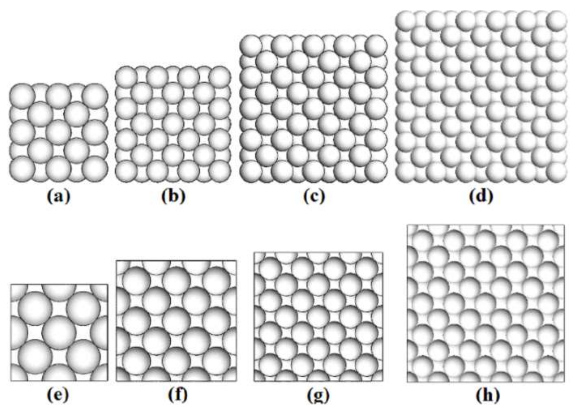
Figure 6.
Body-centered cubic (BCC) samples; named as (a) 1; (b) 2; (c) 3; (d) 4; (e) 1cut; (f) 2cut; (g) 3cut; (h) 4cut.
Figure 6.
Body-centered cubic (BCC) samples; named as (a) 1; (b) 2; (c) 3; (d) 4; (e) 1cut; (f) 2cut; (g) 3cut; (h) 4cut.
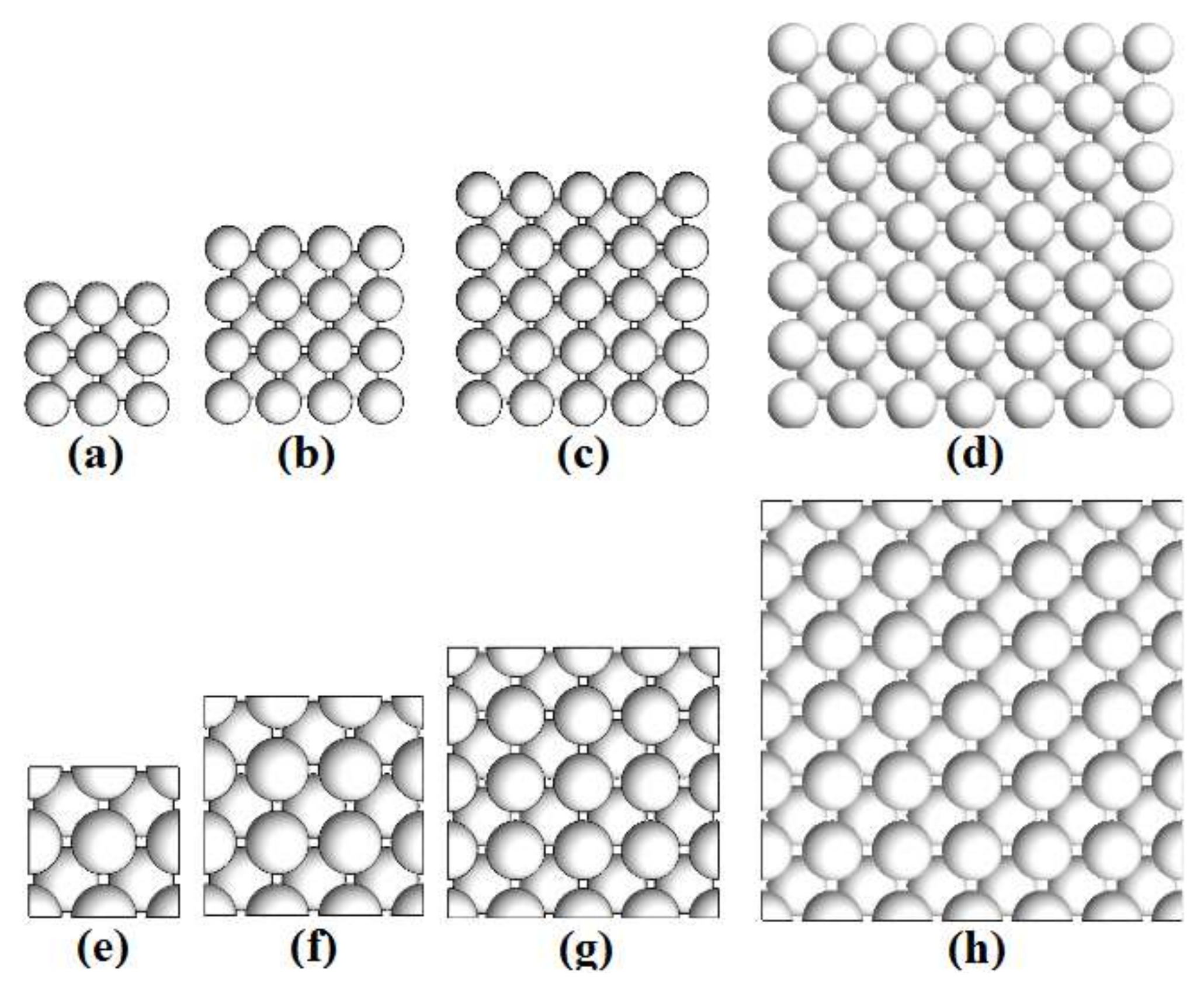
Figure 7.
Voids near the wall.

Figure 8.
Different control volume size by different refinements levels [32].
Figure 8.
Different control volume size by different refinements levels [32].
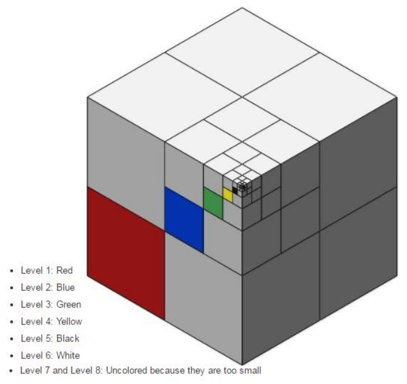
Figure 9.
(a) Calculated volume in flow simulation for three bed structures as a function of mesh level; (b) Pressure drop for three bed structures as a function of mesh level.
Figure 9.
(a) Calculated volume in flow simulation for three bed structures as a function of mesh level; (b) Pressure drop for three bed structures as a function of mesh level.
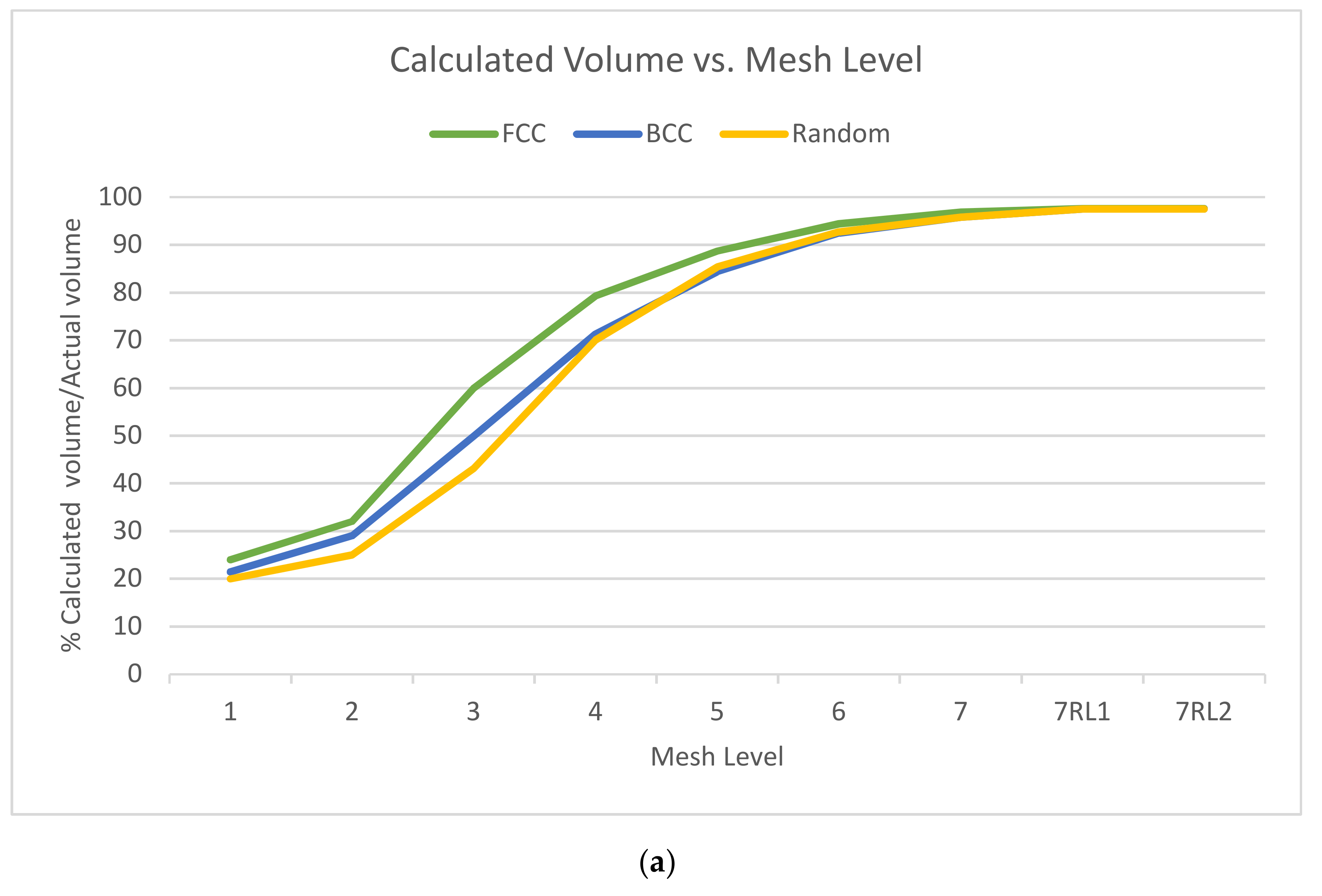

Figure 10.
Random model meshes for (a) initial mesh level 7; (b) initial mesh level 7 with 1 refinement level.
Figure 10.
Random model meshes for (a) initial mesh level 7; (b) initial mesh level 7 with 1 refinement level.

Figure 11.
3D cut models of 3 structures (a) BCC; (b) FCC; (c) random.
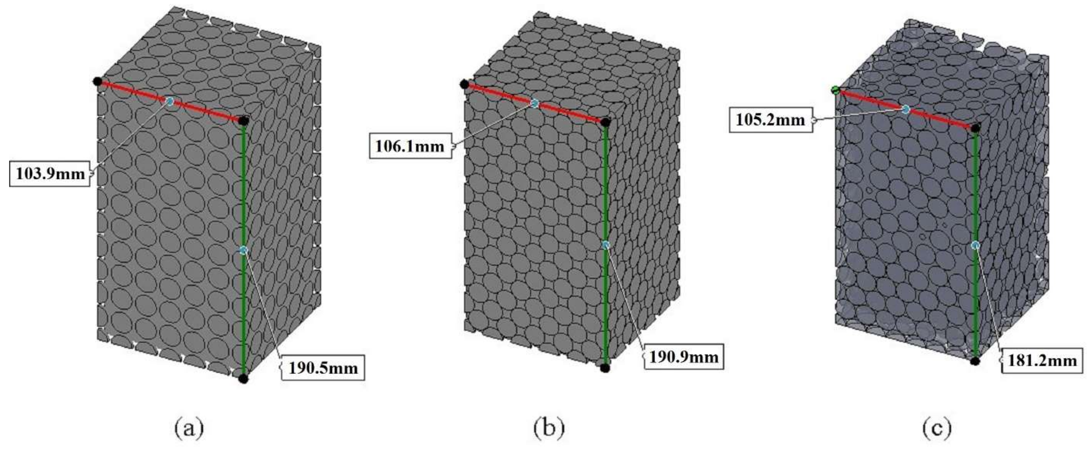
Figure 12.
Flow streaklines from front plane cut plot (a) BCC; (b) FCC; (c) random.

Figure 13.
Velocity distribution from front plane cut plot (a) BCC; (b) FCC; (c) random.

Figure 14.
Pressure drop as a function of velocity for water at 20 °C and 160 bar in 15 mm random model.
Figure 14.
Pressure drop as a function of velocity for water at 20 °C and 160 bar in 15 mm random model.

Figure 15.
(a) Pressure drop as a function of velocity at 3 bed structures with 15 and 20 mm spheres; (b) Percentage difference in pressure drops as a function of velocity.
Figure 15.
(a) Pressure drop as a function of velocity at 3 bed structures with 15 and 20 mm spheres; (b) Percentage difference in pressure drops as a function of velocity.
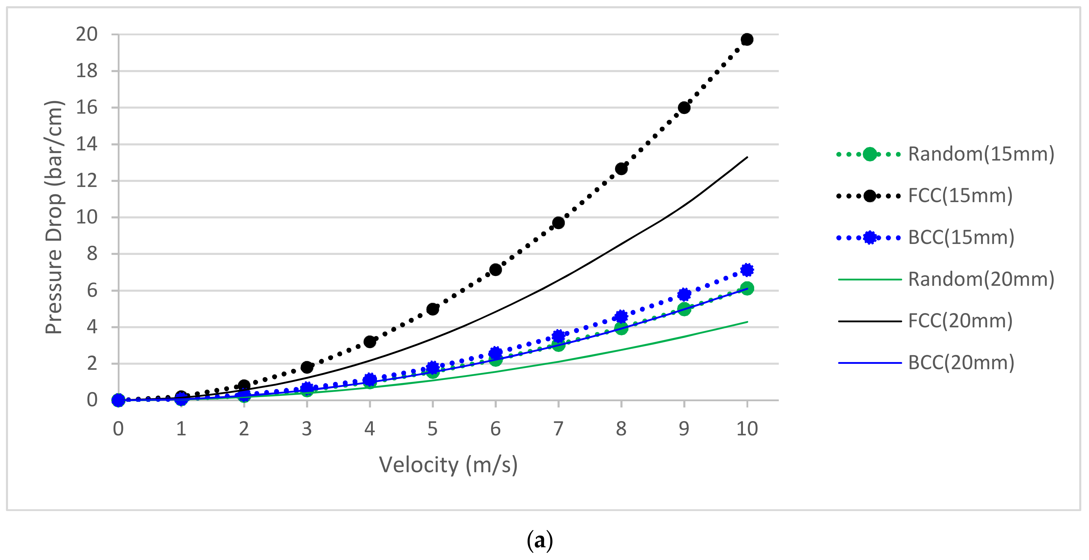

Figure 16.
Pressure drop as a function of velocity for water at three bed structures with 15 mm spheres.
Figure 16.
Pressure drop as a function of velocity for water at three bed structures with 15 mm spheres.
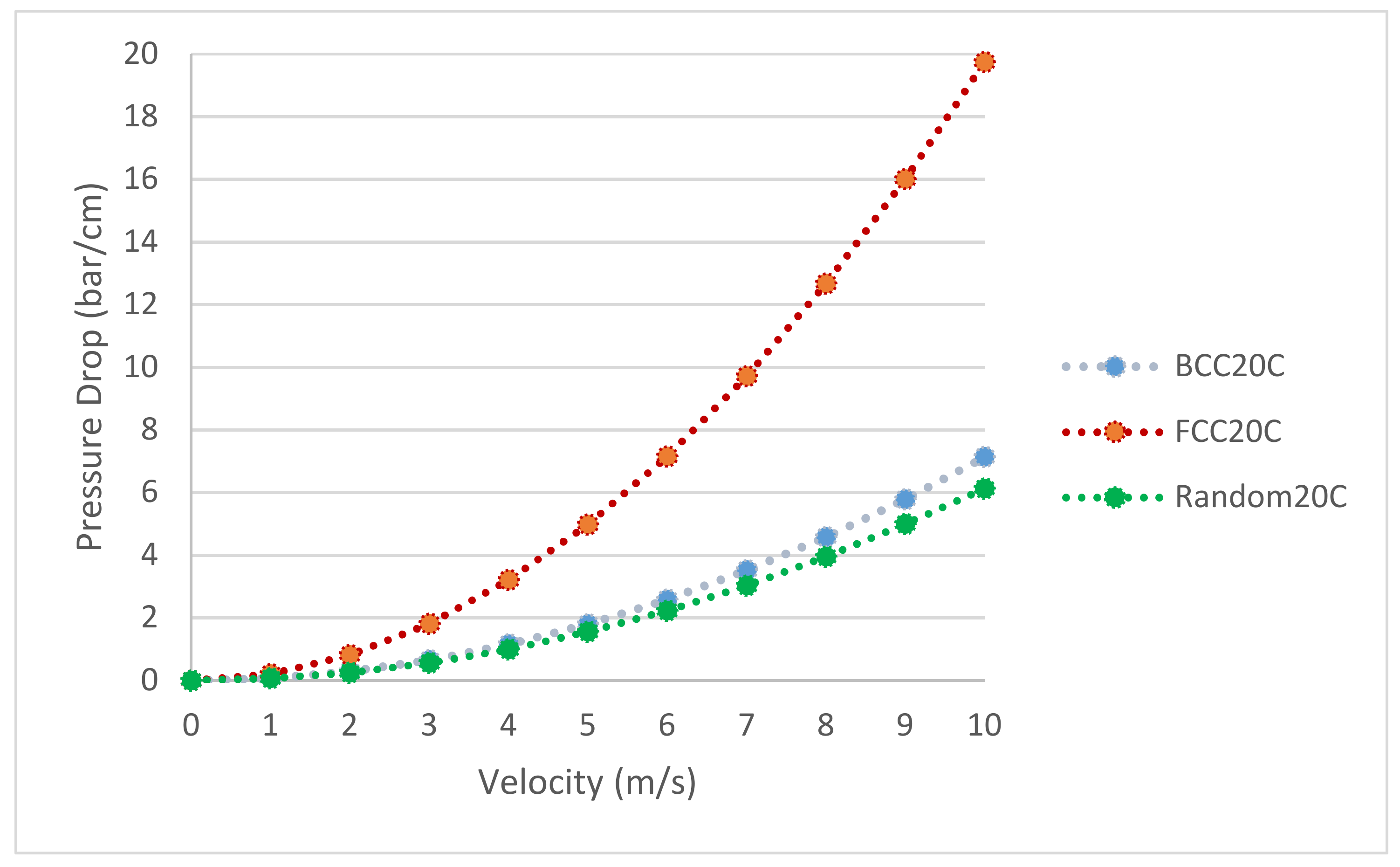
Figure 17.
Pressure drop as a function of velocity at three bed structures and fluid temperatures with 15 mm spheres.
Figure 17.
Pressure drop as a function of velocity at three bed structures and fluid temperatures with 15 mm spheres.

Figure 18.
Change of inertial and viscous forces parts of the Ergun equation by velocity.
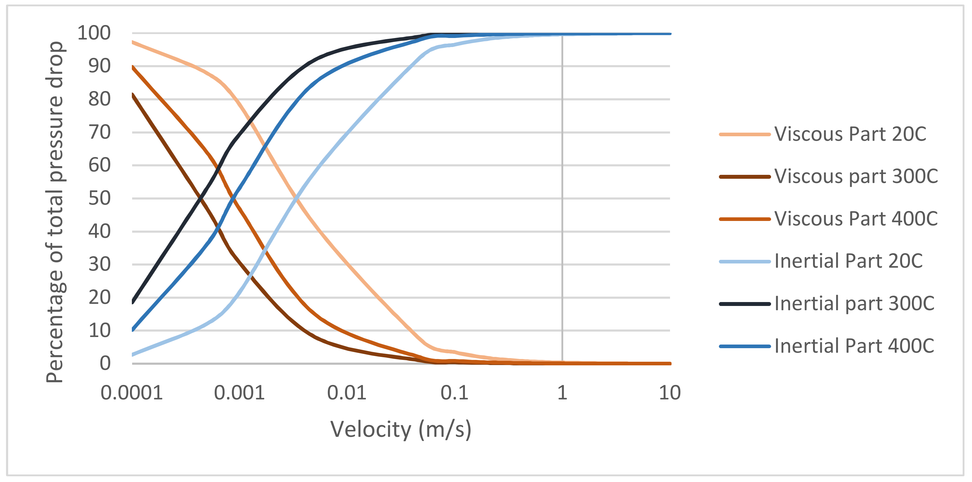
Figure 19.
Pressure drop calculation method comparison for random packing of 15 mm spheres (a) 20 °C; (b) 300 °C; (c) 400 °C.
Figure 19.
Pressure drop calculation method comparison for random packing of 15 mm spheres (a) 20 °C; (b) 300 °C; (c) 400 °C.
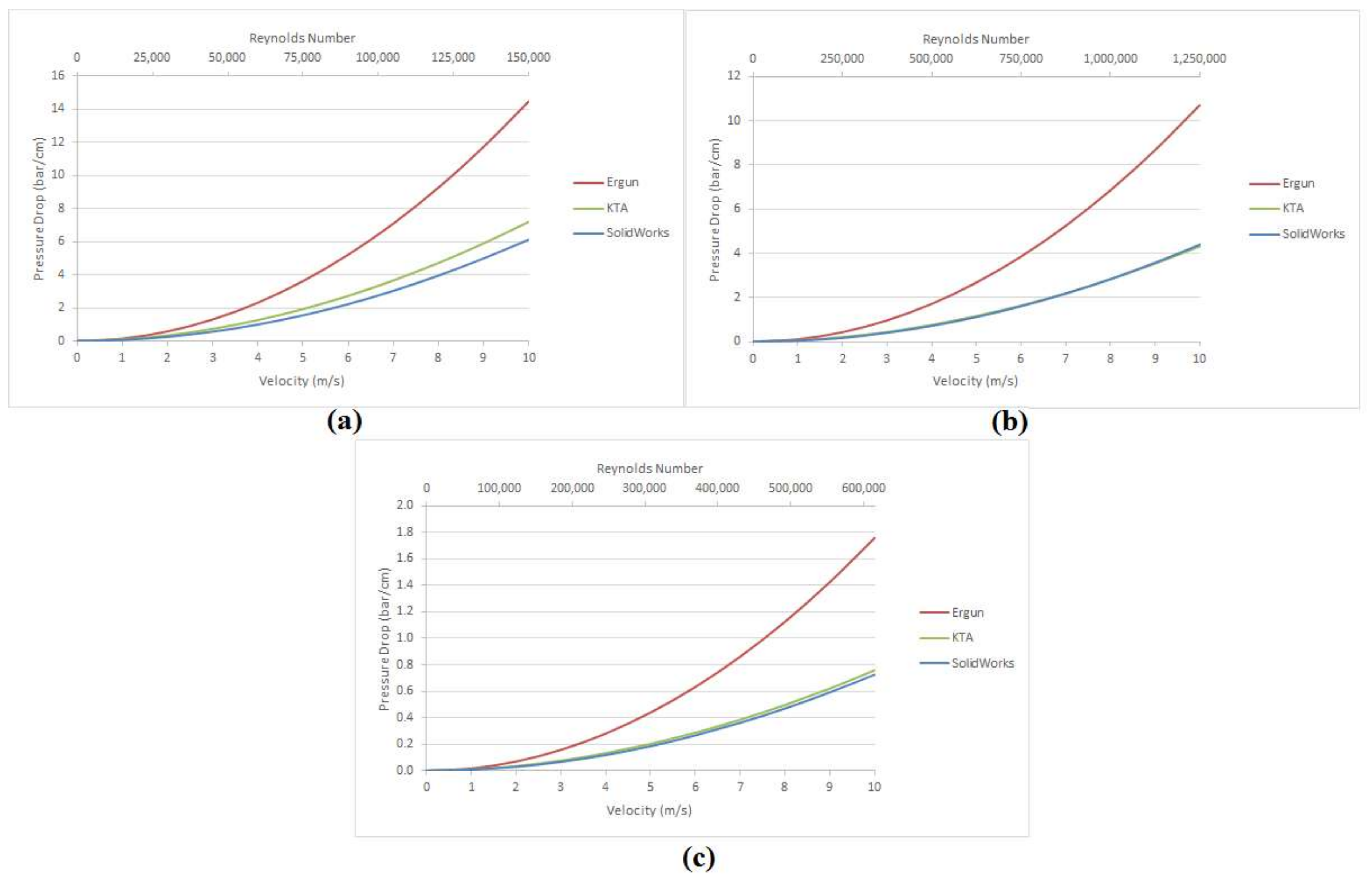
Figure 20.
Predicted and calculated friction factors for PDTS 036 homogeneous porosity test section [41].
Figure 20.
Predicted and calculated friction factors for PDTS 036 homogeneous porosity test section [41].

Figure 21.
SolidWorks results compared with expected pressure drop with new provided equation.
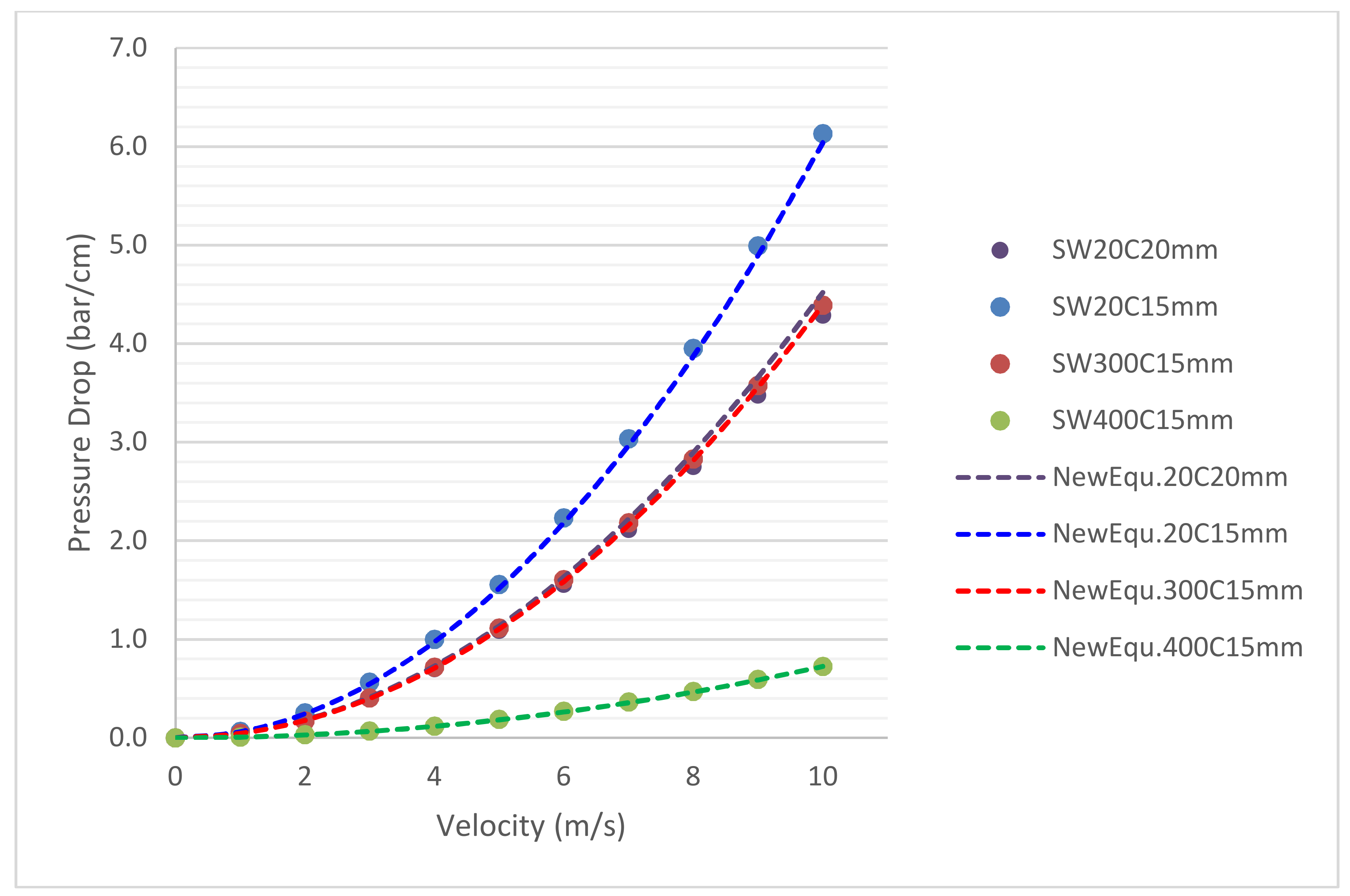
Figure 22.
Required pump power to penetrate different bed structures formed with 15 mm spheres in various temperature of water.
Figure 22.
Required pump power to penetrate different bed structures formed with 15 mm spheres in various temperature of water.


Table 1.
Pressure drops of 8 models for BCC and FCC model for water at 20 °C flowing with 1 m/s velocity.
Table 1.
Pressure drops of 8 models for BCC and FCC model for water at 20 °C flowing with 1 m/s velocity.
| Model Name | BCC Pressure Drop | FCC Pressure Drop |
|---|---|---|
| # | (Bar/cm) | (Bar/cm) |
| 1 | 0.028 | 0.051 |
| 2 | 0.031 | 0.070 |
| 3 | 0.030 | 0.092 |
| 4 | 0.038 | 0.108 |
| 1cut | 0.079 | 0.210 |
| 2cut | 0.084 | 0.200 |
| 3cut | 0.080 | 0.192 |
| 4cut | 0.076 | 0.206 |
Table 2.
Study mesh level accuracy by calculating the volume of bed in three structures.
| Mesh Level | BCC Structure | FCC Structure | Random Structure | ||||||
|---|---|---|---|---|---|---|---|---|---|
| Total Cells | Volume of Bed | Error | Total Cells | Volume of Bed | Error | Total Cells | Volume of Bed | Error | |
| # | m3 | % | # | m3 | % | # | m3 | % | |
| 1 | 1416 | 3.14 × 10⁻⁴ | 78.5 | 772 | 3.16 × 10⁻⁴ | 78.4 | 720 | 4.12 × 10⁻⁴ | 69.9 |
| 2 | 1852 | 3.10 × 10⁻⁴ | 78.8 | 1138 | 4.13 × 10⁻⁴ | 71.8 | 1100 | 4.45 × 10⁻⁴ | 67.5 |
| 3 | 17,519 | 7.31 × 10⁻⁴ | 50.1 | 20,370 | 9.27 × 10⁻⁴ | 36.6 | 18,148 | 7.39 × 10⁻⁴ | 46 |
| 4 | 40,394 | 1.04 × 10⁻³ | 28.7 | 40,583 | 1.22 × 10⁻³ | 16.7 | 37,647 | 1.03 × 10⁻³ | 24.6 |
| 5 | 103,817 | 1.23 × 10⁻³ | 15.6 | 100,204 | 1.43 × 10⁻³ | 15 | 95,462 | 1.21 × 10⁻³ | 11.4 |
| 6 | 257,921 | 1.35 × 10⁻³ | 7.5 | 248,801 | 1.55 × 10⁻³ | 7.6 | 239,610 | 1.29 × 10⁻³ | 6.1 |
| 7 | 548,240 | 1.40 × 10⁻³ | 4.2 | 527,104 | 1.61 × 10⁻³ | 4.3 | 512,761 | 1.31 × 10⁻³ | 4.2 |
| 7RL1 * | 2,540,880 | 1.43 × 10⁻³ | 2.5 | 2,377,161 | 1.64 × 10⁻³ | 2.5 | 2,434,841 | 1.33 × 10⁻³ | 2.5 |
| 7RL2 ** | 11,202,105 | 1.43 × 10⁻³ | 2.5 | 10,480,300 | 1.64 × 10⁻³ | 2.5 | 10,734,605 | 1.33 × 10⁻³ | 2.5 |
| Exact *** | - | 1.46 × 10⁻³ | 0 | - | 1.68 × 10⁻³ | 0 | - | 1.37 × 10⁻³ | 0 |
* 7RL1 stands for 7 initial mesh level and one level of refinement after converging. ** 7RL2 stands for 7 initial mesh level and two level of refinement after converging. *** Exact means the volume calculated without meshing, this data has been obtained by Mass Properties section of SolidWorks.
Table 3.
Porosities of three bed structures.
| Reported Values in Literature | SolidWorks Models | |||||
|---|---|---|---|---|---|---|
| Structure | Packing Factor | Porosity | Nu. of Spheres | Volume of Spheres | Volume of Bed | Porosity |
| FCC | 0.74 [35] | 0.26 [35] | 899 | 1590 cm3 | 2148 cm3 | 0.26 |
| BCC | 0.68 [35] | 0.32 [35] | 792 | 1400 cm3 | 2058 cm3 | 0.32 |
| Random | 0.6366 [36] | 0.3634 [36] | 719 | 1270 cm3 | 2004 cm3 | 0.37 |
Table 4.
Thermodynamic properties of water, imported from HYSYS to SolidWorks.
| Fluid | Density | Viscosity | Heat Capacity | Thermal Conductivity |
|---|---|---|---|---|
| kg/m3 | kg/m.s | kJ/kg °C | W/m °C | |
| Sat. water at 20 °C | 998 | 1.002 × 10⁻³ | 4.183 | 0.6034 |
| Sat. water at 300 °C | 712 | 9.012 × 10⁻⁵ | 5.763 | 0.5411 |
| Supercrtical steam at 400 °C and 220 bar | 121.2 | 2.961 × 10⁻⁵ | 8.169 | 0.1244 |
Table 5.
Pressure drop of water at three different temperatures, flowing in three bed structures.
| Velocity (m/s) | ΔP (Bar/cm) | ||||||||
|---|---|---|---|---|---|---|---|---|---|
| BCC | FCC | Random | |||||||
| Temperature | 20 °C | 300 °C | 400 °C | 20 °C | 300 °C | 400 °C | 20 °C | 300 °C | 400 °C |
| 1 | 0.075 | 0.053 | 0.009 | 0.206 | 0.156 | 0.024 | 0.065 | 0.046 | 0.008 |
| 2 | 0.292 | 0.211 | 0.035 | 0.808 | 0.603 | 0.096 | 0.253 | 0.169 | 0.030 |
| 3 | 0.651 | 0.471 | 0.078 | 1.808 | 1.302 | 0.215 | 0.564 | 0.403 | 0.067 |
| 4 | 1.148 | 0.839 | 0.139 | 3.201 | 2.205 | 0.380 | 0.997 | 0.714 | 0.119 |
| 5 | 1.795 | 1.307 | 0.216 | 4.986 | 3.255 | 0.592 | 1.555 | 1.115 | 0.186 |
| 6 | 2.578 | 1.872 | 0.310 | 7.153 | 4.395 | 0.850 | 2.230 | 1.605 | 0.268 |
| 7 | 3.517 | 2.547 | 0.422 | 9.716 | 5.583 | 1.155 | 3.035 | 2.180 | 0.363 |
| 8 | 4.584 | 3.338 | 0.550 | 12.669 | 6.788 | 1.507 | 3.950 | 2.830 | 0.470 |
| 9 | 5.778 | 4.220 | 0.695 | 16.006 | 7.988 | 1.904 | 4.990 | 3.575 | 0.593 |
| 10 | 7.131 | 5.202 | 0.857 | 19.734 | 9.171 | 2.348 | 6.130 | 4.391 | 0.726 |
Table 6.
Pressure drop, density, and viscosity ratios.
| 20 °C/300 °C | 300 °C/400 °C | 20 °C/400 °C | ||||||
|---|---|---|---|---|---|---|---|---|
| ΔP Ratio | ρ Ratio | µ Ratio | ΔP Ratio | ρ Ratio | µ Ratio | ΔP Ratio | ρ Ratio | µ Ratio |
| 1.48 | 1.35 | 11.12 | 5.75 | 6.09 | 3.04 | 8.37 | 8.23 | 33.85 |
Table 7.
Pressure drop test section (PDTS) information.
| Test Section | D1 * (mm) | D2 ** (mm) | D3 *** (mm) | εavg with Spacers | εavg without Spacers | No. of Particles |
|---|---|---|---|---|---|---|
| PDTS 036 | 741.1 | 300 | 300 | 0.352 | 0.369 | 3445 |
| PDTS 039 | 756.46 | 300 | 300 | 0.389 | 0.407 | 3307 |
| PDTS 045 | 781.7 | 300 | 300 | 0.448 | 0.465 | 3080 |
* D1 represents height of the model. ** D2 represents depth of the model. *** D3 represents width of the model.
Table 8.
Percentage difference between predicted and experimental friction factors [41].
Table 8.
Percentage difference between predicted and experimental friction factors [41].
| Reynolds Number | KTA Deviation from Experimental Data (%) | ||
|---|---|---|---|
| PDTS 036 | PDTS 039 | PDTS 045 | |
| 1000 | 9.4 | 20.6 | 56.0 |
| 2000 | 23.8 | 38.0 | 80.7 |
| 3000 | 35.9 | 49.2 | 97.5 |
| 4000 | 44.1 | 59.4 | 110.7 |
| 5000 | 51.5 | 68.5 | 125.7 |
| 6000 | 59.5 | 76.9 | 137.4 |
| 7000 | 66.6 | 84.6 | 148.5 |
| 8000 | 72.5 | 91.7 | 158.5 |
| 9000 | 78.5 | 98.4 | 168.0 |
| 10,000 | 63.5 | 104.9 | 176.9 |
| 20,000 | 126.6 | 152.5 | 252.3 |
| 30,000 | 139.5 | 173.3 | 291.1 |
| 40,000 | 143.2 | 185.8 | 315.6 |
| 50,000 | 140.7 | 190.1 | 327.7 |
Table 9.
The description and results of the mesh independency (MD) tests.
| Case | Number of Cells (×106) | Pressure Drop | CFD Deviation from KTA |
|---|---|---|---|
| - | # | (Pa) | (%) |
| MD-1 | 1.878 | 11.4668 | 10.87 |
| MD-2 | 2.632 | 11.7734 | 8.49 |
| MD-3 | 3.901 | 12.0909 | 6.03 |
| MD-4 | 5.1695 | 12.358 | 3.45 |
| MD-5 | 8.6466 | 12.6746 | 1.49 |
| MD-6 | 9.655 | 12.7165 | 1.16 |
| MD-7 | 12.7862 | 12.833 | 0.25 |
| MD-8 | 15.4180 | 12.9123 | 0.36 |
© 2018 by the authors. Licensee MDPI, Basel, Switzerland. This article is an open access article distributed under the terms and conditions of the Creative Commons Attribution (CC BY) license (http://creativecommons.org/licenses/by/4.0/).
Share and Cite
MDPI and ACS Style
Ahmadi, S.; Sefidvash, F. Study of Pressure Drop in Fixed Bed Reactor Using a Computational Fluid Dynamics (CFD) Code. ChemEngineering 2018, 2, 14. https://doi.org/10.3390/chemengineering2020014
AMA Style
Ahmadi S, Sefidvash F. Study of Pressure Drop in Fixed Bed Reactor Using a Computational Fluid Dynamics (CFD) Code. ChemEngineering. 2018; 2(2):14. https://doi.org/10.3390/chemengineering2020014
Chicago/Turabian StyleAhmadi, Soroush, and Farhang Sefidvash. 2018. "Study of Pressure Drop in Fixed Bed Reactor Using a Computational Fluid Dynamics (CFD) Code" ChemEngineering 2, no. 2: 14. https://doi.org/10.3390/chemengineering2020014