Article

Water Balance to Recharge Calculation: Implications for Watershed Management Using Systems Dynamics Approach

1
School of Engineering, University of California, Merced, CA 95343, USA
2
Department of Civil Engineering, University of Idaho, Moscow, ID 83844, USA
*
Author to whom correspondence should be addressed.
Hydrology 2016, 3(1), 13; https://doi.org/10.3390/hydrology3010013
Submission received: 16 November 2015 / Revised: 6 March 2016 / Accepted: 8 March 2016 / Published: 18 March 2016

Abstract

:
Groundwater depletion in the face of growth is a well-known problem, particularly in those areas that have grown to become dependent on a declining resource. This research comprises a broad synthesis of existing water resources data, to understand the long-term implications of continued growth in water demand on groundwater dominant water resources, and to develop a tool for sustainable water management. The Palouse region of Washington and Idaho, USA. (approximately 60,000 people in a rural setting) is entirely dependent on groundwater from two basalt aquifers for potable water. Using the systems dynamics approach and a water balance that considered the entire hydrologic cycle, a hydrologic model of these aquifers was developed, tested and applied to simulate their behavior over a 150 year time period assuming the current infrastructure does not change. With 1% population growth and current water extraction rates, the results indicated the upper aquifer use may be sustainable, while the lower aquifer use is likely unsustainable in the long term. This study also shows that uncertainties in key aspects of the system create limitations to groundwater management.

1. Introduction

The continuing extraction of groundwater from the aquifers for drinking, agricultural and industrial usage is contributing to groundwater depletion in many parts of the United States and the world [1,2,3,4,5,6,7,8,9,10,11]. Managing groundwater with limited information is complicated, and dealing with uncertainties not only requires significant scientific effort, but can lead to ineffective management that is slow to respond to observed depletion. Information is generally limited because of complex hydrogeology, difficulties in and costs of data collection, and the need for frequent monitoring. For example, recharge is considered to be one of the most difficult components of a water-balance to quantify accurately as it varies significantly in both temporal and spatial dimensions [12,13,14,15,16,17,18,19]. Effective management of groundwater aquifers is heavily influenced by the accurate estimation of recharge. Another, perhaps under-appreciated characteristic of large confined aquifers that affects long-term management is storativity, as it defines the volume of water that is or could be stored for future use. Together, recharge and storativity and their uncertainty are critical for groundwater management.
The Palouse region is a semi-arid area located along the border of northern Idaho and eastern Washington, is solely dependent on groundwater for drinking water. Two distinct confined groundwater aquifer systems exist in the Palouse Basin (PB), the upper Wanapum (WP), and the lower Grande Ronde (GR). The GR aquifer supplies the potable water for approximately 70 percent of Moscow, Idaho and 100 percent of Pullman, Washington. The WP aquifer is on average 110 m below ground surface and is thought to receive some recharge, while the GR aquifer is on average approximately 290 m below ground surface with indeterminate recharge rates. Since the first well was installed over 100 years ago, water levels in the GR have been decreasing 0.3–0.45 m annually indicating long-term unsustainable use [20]. Much effort has been expended to understand basin hydrogeology and groundwater recharge of the PB (e.g., [21,22,23,24,25,26,27,28,29,30,31]). To estimate basin-scale recharge of the PB, Dhungel [29], conducted a water balance at the land surface based on 30-year average precipitation, streamflow, and evapotranspiration; it is assumed that this recharge is received by the upper WP. The lower GR is often thought to receive little to no recharge. This assumption is supported by some studies ([28] and [32] but many believe the existence of recharge to GR ([26,33,34,35]).
In the 1950s, the systems dynamics method was formally created by J. W. Forrester at Massachusetts Institute of Technology [36], which has proved to be useful to simulating any system that can be thought of in terms of stocks and flows. The approach is often used for shared vision planning of natural resources, a process which involves discussion and debates as part of the comprehensive decision making process [37]. The systems dynamics approach facilitates understanding of the behavior of complex systems over time. As such, the use of systems dynamics in water resources planning accelerated in the 1990s, for example in water resource planning [38,39,40,41,42,43,44,45,46,47,48,49] and for groundwater management [50,51,52]. Mirchi et al. [53] synthesized the integrated water resources modeling efforts. Dhungel [29] and Beall et al. [45] discussed water resources management efforts in the Palouse region using a systems approach.
Thus, the overall objective of this study was to synthesize the currently available hydrologic data, and to incorporate the results of this synthesis as a lumped water balance model using a systems dynamics approach. This model is then used to simulate future water resources for various growth scenarios and to show the effects of uncertainties.

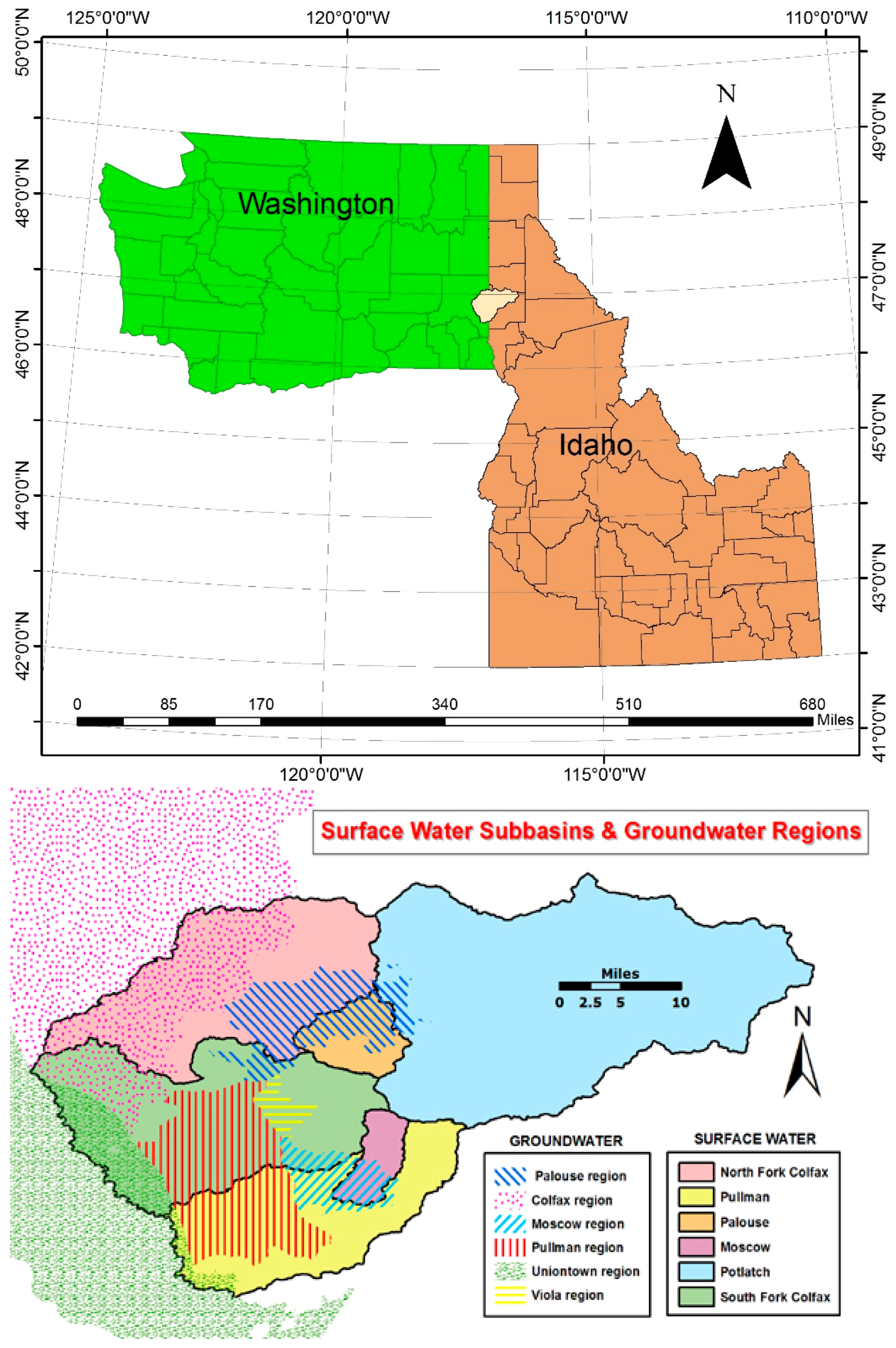
2. Study Area and Data

The majority of land in the Palouse Basin is used for dryland agriculture (grains and legumes) and forest. The soils are primarily silty loam loess, wind-transported soils that form rolling hills, which overlies Columbia River basalt flows. Palouse loess elevations range from 1010 m along the eastmost boundary to 520 m in the west. The climate is semi-arid, with precipitation falling primarily in the winter months, and the summers are relatively hot and dry. The total population of Palouse region was about 51,000 (2006) which is comprised of small cities like Moscow, Potlatch, Pullman, Viola, Potlatch, and Colfax. Approximately 9.5 percent of the total water demand of the PB was fulfilled by the WP and rest by the GR. Total water extraction from the PB was about 2.77 billion gallons in the year 2005 [54]. Water extraction from the GR (2.51 billion gallons/year) was approximately nine times greater than the WP (0.26 billion gallons per year) in the year 2005. The per capita per day water use of the PB is approximately about 150–180 gallons [20,21], but recent studies show a decline in water use, which is about 120 gallons [55] that is used in the simulation.
Population data are acquired from the United States Census Bureau and city sources. The population of this area is estimated to grow by 1% annually [20]. A longer simulation period, i.e., 150 years were chosen in contrary of 50–100 years because it is assumed that the population growth of these rural settings would rise constantly rather than a large spike. Figure 1 shows the location map of the study area and groundwater and surface area regions. The groundwater aquifers of PB are located within the basaltic Columbia River flows. Water level of principal well in the basin is about 686 m (above mean sea level) in 1990s [56]. Even though, there is water below 488 m (i.e., 1600 ft) but uncertainty of water volume increases significantly [45]. The existence of the upper WP aquifer seems significant in all groundwater basins with comparatively thin layer in Pullman (46 m) [57]. The Moscow WP is productive for groundwater extraction whereas the Pullman WP is unproductive [58]. The uppermost layer of the Palouse Basin is composed of loess which is basically a deposit of wind-blown silt. The composition of these aquifers is more than 60 percent basalt, with the rest being sediments including silt, clay and sand. According to the geographic variations, the groundwater regions are divided into Palouse, Colfax, Viola, Pullman, Moscow and Uniontown regions (Figure 1, [57]). The radiocarbon age of GR groundwater basin varies between 8500 and 31,000 years apparent Radiocarbon Age (BP) [32], between 13,000 and 26,400 years (BP) for the lower portion of the GR and 4400 to 11,800 (BP) for upper portion of the GR [59] and approximately 20,000 years [45].
The question of the storativity of the basaltic rock of PB aquifer and Columbia basin is a particular interest of geologist, water managers and hydrologist. The two closely located state universities of Idaho and Washington along with other entities are working to better understand the aquifer properties and hydrogeology of the basin. Studies show that storativity of PB aquifer basalt ranges approximately between 10−3 and 10−5 based on aquifer discharge tests [60], 1.5 × 10⁻⁴ ± 0.2 × 10⁻⁴ [61], 3 × 10⁻⁵ to 3 × 10⁻⁴ of GR [62] and 0.67 × 10⁻³ of WP [63]. Moran [62] had compiled the storativity estimates from previous PB investigations. Even though the storativity values of the aquifer are vital because it governs the initial volume and overall life of aquifers, recharge to the aquifers plays a critical role. The short term drawdown and recovery (1930–1990) of WP indicates that recharge was the prevailing factor of the dynamics of WP. The aquifer recharging process can be less evident in GR because of the larger surface area, complex hydrology, and hydraulic and hydrologic connectivity among the other groundwater regions, but the inconsistency between the drawdown and extraction is indicating that GR might be actively recharging. Analyzing initial volume of aquifers, the current decline rate the aquifer and the long term pumpage, we utilized the storativity value of 10−3–10−4 [61] for the modeling purposes. Smaller storativity values imply less water stored in the specific saturated depth of aquifer as well as only a little amount of water that can be extracted from drawdown.
To conduct basin scale water balance, different sets of climatic and surface water data is needed. For calculating evapotranspiration, land use maps, soil maps, elevation maps and PRISM maps [64] were used. To compute the surface water, daily discharge from USGS gauging stations was used from 1970 to 2000. A watershed was delineated using 10 m resolution Digital Elevation Map (DEM) of PB. Colfax (i.e., USGS gauging station 13346100, Palouse River at Colfax, WA) was taken as the downstream point for delineating watershed. Five more USGS gauging stations were used for delineating sub-watersheds with a total area of 2044 km2 representing entire PB (Table 1). The basin was divided into six surface water sub-basins defined by the United State Geological Survey (USGS) surface water gauging station locations (Figure 1).

3. Methodology

In this section, discussions are carried out of the components of the water balance, governing equations and the applied boundary conditions.

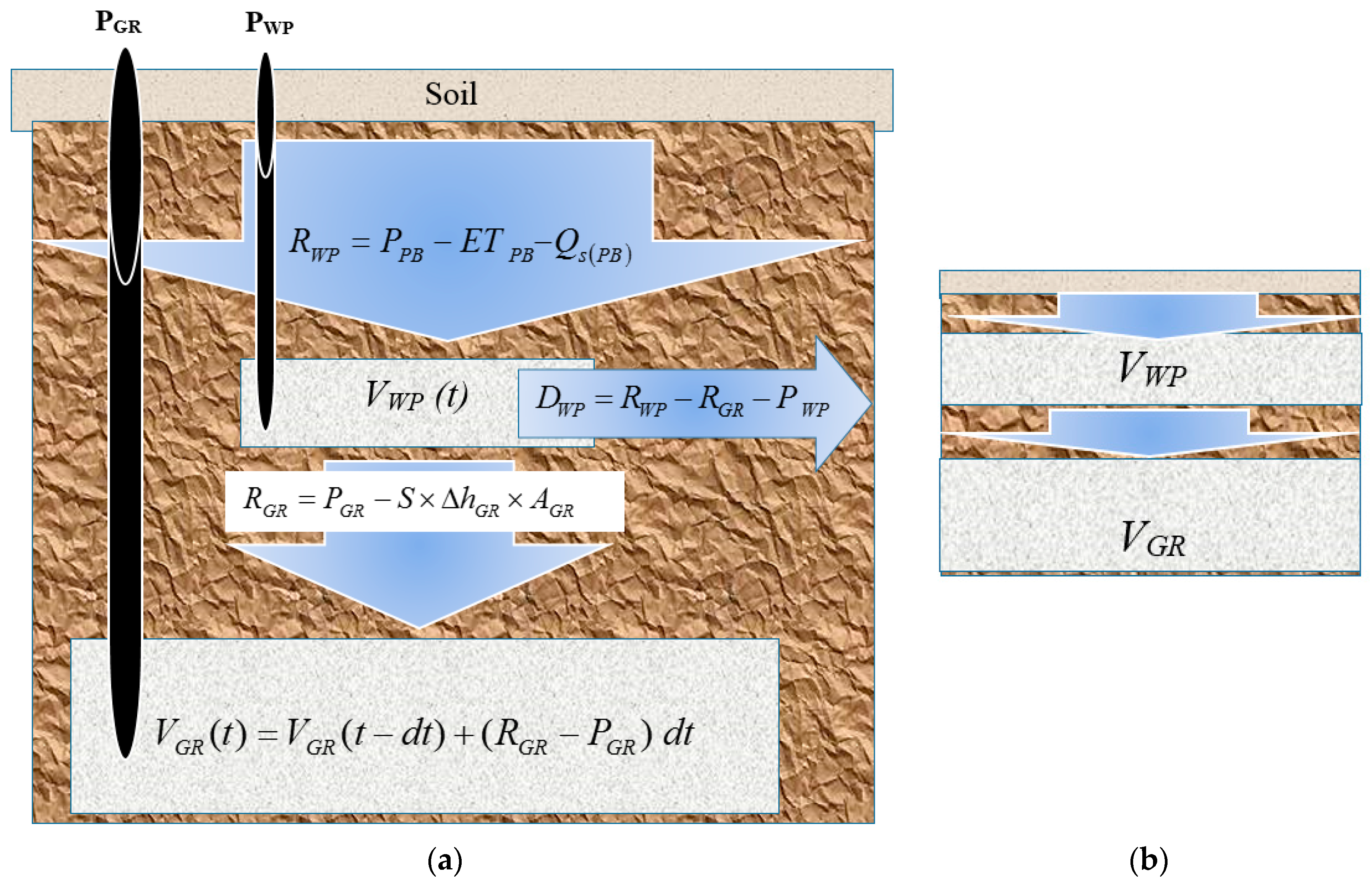
3.1. Water Balance Analysis

The hydrology section is divided into surface water and groundwater. Surface water hydrology is described by mean annual precipitation, surface runoff and evapotranspiration; recharge is computed by water-balance, assuming that the average soil moisture storage change in the unsaturated zone is zero. Equation (1) shows a general form of the water-balance approach used to calculate recharge to WP [65,66,67,68]. The recharge was calculated using the basic water-balance approach over the 1971 to 2000 time period (2044 km2). Scanlon et al. [12] classified recharges broadly as physical based and tracer or numerical modeling approach. Scanlon et al. [69] categorized the techniques for estimating recharge for surface water, unsaturated zones, and saturated zones. Risser et al. [70] used unsaturated-zone drainage collected in gravity lysimeters, daily water balance, water-table fluctuations in wells, and equations of Rorabaugh for estimating ground-water recharge at a humid-continental climate in east-central Pennsylvania. Lee et al. [71] discussed the standard techniques for regional groundwater recharge calculation based on water-balance model and parameter-value adjustment of groundwater flow models. Simmers [72] defined recharge as short-term, seasonal, perennial and historical based on the different time scales. A water budget or balance approach is the largest class techniques to estimate recharge [73].
P P B E T P B   Q s ( P B ) Δ S P B = R W P   [ L 3 / T ]
The term P (L3/T) represents precipitation, ET (L3/T) is the evapotranspiration, Qs (L3/T) is the discharge of the river (surface water inflow), ΔS (L3/T) is storage change in the unsaturated zone, and R (L3/T) is the recharge.
Mean areal annual precipitation in Equation (1) was computed from Parameter-elevation Regressions on Independent Slopes Model (PRISM) maps of girded data with 30-arcsec (800 m) NORMALS (1971–2000). The estimation of evapotranspiration in equation 1 followed the prediction methodology by the Thornthwaite and J.R. Mather approach. Thornthwaite-Mather [74] is a lumped model where the entire watershed is treated as a single unit and soil water status is tracked through time. Specific parameters used in this method are rooting depth, available soil water storage depth, crop coefficient and maximum canopy storage amount. The potential evapotranspiration was calculated using the Hargreaves approach [75]. Daily discharge data (1971–2000) from the USGS gauging stations were used to calculate surface runoff (Equation (1)). Surface water watersheds are delineated solely from USGS gauging station locations in order to perform mass-balance computations. Table 1 also includes the USGS gauging stations, period of data availability and the linear regression equations that are used to estimate missing data such that the water balance is based on a consistent period of record.
The groundwater volume of the aquifers (V (L3)) were estimated from potential groundwater drawdown of average saturated depth (H (L)), surface area of the aquifer (A (L2)) and storativity (S) [76].
V = S   × A ×   H   [ L 3 ]
Water-balance of WP (Equation (3)) is computed by balancing the initial volume of WP (VWP, Equation (2)), recharge to WP (RWP), discharge from WP (DWP) that does not reach to GR, WP pumpage (PWP), and recharge to GR (RGR). It is assumed that about 12% of water is extracted from Wanapum and rest from GR.
V W P ( t ) = V W P ( t d t ) + ( R W P P W P R G R D W P )   d t   [ L 3 / T ]
Change in storage in WP (ΔSWP) can be written as of Equation (4).
V W P ( t ) V W P ( t d t ) = Δ S W P = 0   ( A f t e r   1990 )   [ L 3 / T ]
In Equation (3), all the components are known except DWP and RGR. Discharge from Wanapum (DWP) that does not reach to GR is computed from the following equation simplifying Equation (3) and (4) (Equation (5)).
D W P = R W P P W P R G R   [ L 3 / T ]
Water-balance of GR is computed by balancing the initial volume of GR (VGR), recharge to GR (RGR), and GR pumpage (PGR). In Equation (6), all the components are known except RGR.
V G R ( t ) = V G R ( t d t ) + ( R G R P G R )   d t   [ L 3 / T ]
Change in storage in GR (ΔSGR) can be written as of Equation (7). The term ΔhGR [L] represents drawdown of GR and AGR is surface area of GR.
V G R ( t ) V G R ( t d t ) = Δ S G R = S × Δ h G R × A G R   [ L 3 / T ]
Recharge to GR can be computed simplifying Equations (6) and (7) (Equation (8)). With this assumption, any discrepancy in estimation of storativity or surface area of GR can affect the overall accuracy of the estimated recharge. Similar approach (Equation (8)) had been utilized to test how the system parameters affect the recharge estimates in GR [61,62]. The maximum recharge to GR (RGR (max)) is limited to 4 cm/year not to surpass the recharge from water balance.
R G R ( max ) = P G R S × Δ h G R × A G R   [ L 3 / T ]
Once the recharge reaches to the maximum value, drawdown can be back calculated using following equation.
Δ h G R ( c a l ) = P G R R G R ( m a x ) S × A G R   [ L / T ]
The simulation process is stopped when GR aquifer no more able to fulfill the entire demand.

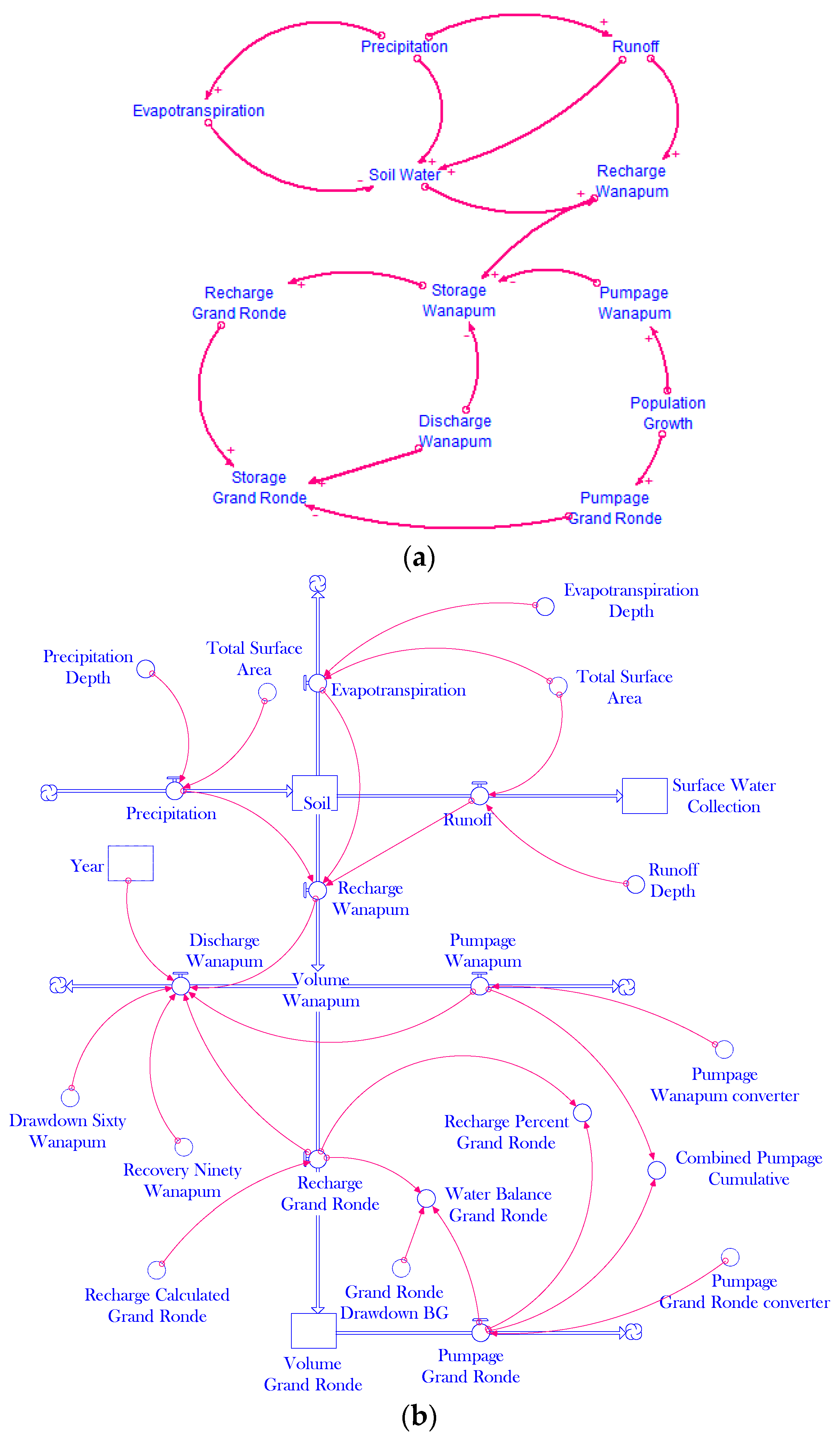
3.2. Modeling Approach

A schematic of the PB watershed is shown in Figure 2a where the surface area of the PB, the productive WP region and GR region varies. These surface area of aquifers is used to compute the initial volume of groundwater, which represents the start of the simulation period which is 1930. Prior to 1930, it is assumed that there was no significant overdraft of groundwater in both aquifers. As it is generally thought that GR get recharged from the fractures, so the actual pathways of recharge to GR is insignificant. GR regions are assumed as non-leaking reservoirs. Studies show the GR aquifer system of the Moscow, Pullman, Colfax and Garfield are hydraulically connected [77]. Based on this finding, we combined the groundwater regions of GR to develop a lumped GR hydrological unit (728 km2, (610 km2 , suggested by [59]) for water storage and water balance purpose. Similarly, lumped WP region is associated with Moscow WP (82 km2) assuming that the rest of WP groundwater regions are unproductive (Figure 2a). If the surface area of WP and GR are assumed to be identical of PB (2044 km2), the groundwater storage and extraction (Figure 2b) will be increased. Simulations will be carried out how these affect the final results.
Figure 3a shows the causal loop diagram of the Palouse basin watershed in its simplest form. An increase in precipitation will increase recharge to WP and GR. Increased population in PB would put pressure to both WP and GR which will ultimately reduce the storage of aquifers by further increasing the drawdown.
A systems model of the PB watershed using STELLA software [78] shown in Figure 3b. Historical and current observations show (1930 to current) that the average annual drawdown of GR is about 0.37 m irrespective of approximately five times population growth (10,000 to 50,000). The annual water level drop in GR actually slightly decreased from 0.45 m to 0.3 m in 1990s. These water level decline trends are indicating that multiple factors (probably recharge, connectivity of groundwater regions, storativity, porosity, resident time, groundwater dating etc.) are influencing along with the population growth. Beall et al. [45] purposed dual porosity to estimate the aquifer decline rate of GR using resident time concept. Dhungel [29] had conducted an extensive sensitivity analysis to understand the aquifer behavior of PB varying storativity, surface area and recharge, but because of the uncertainty in recharge and storativity values, the effort provided a little insight to understand the life of these aquifers. In this study, we utilized the indirect substitution method rather direct sensitivity analysis to estimate recharge to GR (Equation (8)). According to Equation (8), GR pumpage constantly exploits WP in the form of recharge to balance the deficit between the GR pumpage and drawdown.
We assumed that the current water depletion trend will continue for a certain period of time in the future, eliminating one of the unknowns in Equation (6), which ultimately helps to calculate recharge to GR. The vital question is if this trend continues, then how long it last and how will it respond to the increased population growth. Obviously, increased population growth will accelerate the groundwater extraction and shorten the life of these aquifers, however, the water decline trend of GR may not be linearly proportional to population growth as we believe there might be active recharge. Our goal here is to develop a model which can sustain the current water decline rate for the existing population growth (1%) as well as the increased growth. The only way it can be achieved is from additional contributions from WP to GR as recharge, but recharge to GR from WP is the function of water balance of PB. The simulation will find out the cutoff point where these water balance equations and the hypothesis are not further applicable. The actual water level trend in the simulation may be less intuitive, but these cutoff points will indicate the optimum duration that this trend can exist with these hypothesis and assumptions. The model will face two types of threshold or cutoff points a) basically when the demand of GR i.e., GR pumpage is higher than GR storage (deficit threshold) b) when the recharge to GR reach the maximum allowed values (recharge threshold).
The drawdown of the groundwater aquifers can vary both spatially and temporally and needs an enormous number of monitoring wells to understand basin scale drawdown. As a part of model validation, we mimicked drawdown behavior of these aquifers based on the historical and current observations. To replicate the drawdown behavior of the WP between 1930 and 1960, a constant drawdown (ΔhWP: approximately 0.1 m/year for 30 years) was adopted. During this period, the majority of water was extracted from the upper WP which generated rapid drawdown in WP. When the extraction from WP was dwindled to overcome this drawdown, the water level of WP started attaining back to an earlier state at 1990s [45]. During this period (1960–1990), increasing ΔhWP was adopted to balance the previous loss. Finally, from 1990s, ΔhWP is considered to be zero as WP is nearly constant. To replicate the GR decline trend, a constant value of ΔhGR (i.e., 0.45 m/year) was adopted between 1930 and 1990 and after 1990, 0.3 m/year.

4. Results and Discussion

4.1. Water-Balance and Recharge to Aquifers

In this section, discussion is carried out of individual component of the water balance of particular sub-watersheds. As we are generating a lumped model, there may little importance of particular components of sub-watersheds, but it is intended to demonstrate how components of water balance can vary in a fairly small watershed. The maximum precipitation value within the watershed is approximately 85 cm in the Palouse River sub-basin above Potlatch, Idaho, while the lowest value of approximately 59 cm is observed at South Fork above Colfax, Washington. The mean areal precipitation over the entire watershed is approximately 71 cm. The maximum mean areal surface runoff is approximately 29 cm in the Palouse River near Potlatch, Idaho, while the lowest value of 5 cm is observed in the Palouse River at Palouse, Washington. The mean areal runoff over the entire watershed is approximately 17 cm. The maximum mean areal ET is approximately 54 cm in the Palouse River near Potlatch, ID, while the lowest value of approximately 45 cm is observed in the South Fork above Colfax, Washington (North Fork). The mean areal ET over the entire watershed is approximately 49 cm. Table 2 shows the estimated surface runoff, evapotranspiration and precipitation of each sub-watershed of WP aquifer. The areal mean precipitation, evapotranspiration and runoff of entire watershed was 71, 49 and 17 cm resulting recharge of 4.7 cm.
The wide variation in calculated recharge from the surface watersheds (Table 2) suggests that replenishment of the underlying WP aquifer would also be spatially variable. Some portions of the WP aquifer will be more easily recharged than others due to differences in recharge rate. To understand these variations, Dhungel [29] developed a hydrologically separated model based the geological separation of groundwater regions. A water-balance at the land surface was used to estimate recharge to the Wanapum by spatially sub-dividing surface water areas and groundwater regions. However, the population center of PB lies within 7 miles i.e., Moscow and Pullman area and the hydrogeological investigations indicated that Moscow WP is only productive, the hydrologically separated model faces similar constraints to the lumped models [29]. Because of significant heterogeneity in the GR, traditional numerical model of groundwater flow (e.g., MODFLOW) had offered little insights into the overall nature of the aquifer [22,45].
Table 3 shows some of the documented WP recharge values based on various approaches since 1960s. These studies suggest the recharge rates of upper WP varies from 0.3 to 19.7 cm/year. The large differences in these recharge calculations increase uncertainty in water storage in WP. Based on the expert elicitation and Bayesian Model, Reeves [30] found the estimated WP areal average recharge to be 5.1 cm·year−1 with an uncertainty of ±4.6 cm·year−1.
Based on the recharge calculation (Table 2), the water-balance shows 383 billion gallons (BG) of water are contributed by precipitation, 93 billion gallons of water are converted into surface runoff, and evapotranspiration accounts for 267 billion gallons, resulting in 22 billion gallons of recharge to the WP for the year 2005. This amount of recharge (approximately 4 centimeters per year) corresponds to an average rate over the entire area of 2044 kilometers. This estimated recharge amount to WP aquifer is approximately eight times larger than the present water extraction of entire PB (2.77 billion gallons, 2005). This may be the possible indication, in part (1) the computed recharge is likely overestimated (2) entire recharged water does not reach to WP (3) GR get constant recharge from WP (4) possible inconsistency of surface areas of PB, WP and GR. The computed recharge from the water-balance is in the range of the previously documented values (Table 3). As per the assumptions, the portion of recharged water might be discharged from WP while the rest might be possibly recharging to GR (Equations (3)–(5)).

4.2. Aquifer Storage

One of the frequently raised questions while managing the groundwater is the aquifer storage capacity and possible life of the aquifers. However, the larger uncertainty in storativity and hydrogeology can put these topics in shadow and the usefulness of these simple models can also be questioned. The estimated total initial volume of the WP and GR is about 0.3 billion gallons (surface area about 82 km2) and about 5 billion gallons (surface area of 728 km2), respectively, when potential drawdown at the bottom of the aquifers with storativity of 10−4 (Table 4). This total volume of groundwater in the WP and GR represents the maximum water in the aquifers irrespective to the present water level. The average maximum potential drawdown of the Moscow WP is about 137 m, Moscow GR is 271 m and Pullman GR is 305 m at the bottom of aquifers. Now, coming back to the original question if these estimated aquifer storage capacity is reasonable, while comparing the actual water extraction. Water extraction from these aquifers far outreaches the estimated storage capacity or our understanding to storativity and recharge needs extensive revisiting.
As an optimistic scenario, simulation was also carried out of the storativity of 10−3 (based on the published storativity values). The higher storativity values not only imply a larger storage capacity, but also a larger amount of water literally extracting from the current drawdown. Similarly, smaller storativity indicates a large amount groundwater needs to be replenished as recharge to balance the current pumpage. The amount of water that is continuously declining from GR is about 0.06 billion gallons (storativity = 0.001, 0.3 m/year) and 0.01 billion gallons (storativity = 0.0001, 0.3 m/year), which is a tiny fraction of the current extraction. It indicates the substantial contribution of recharge in both scenarios.

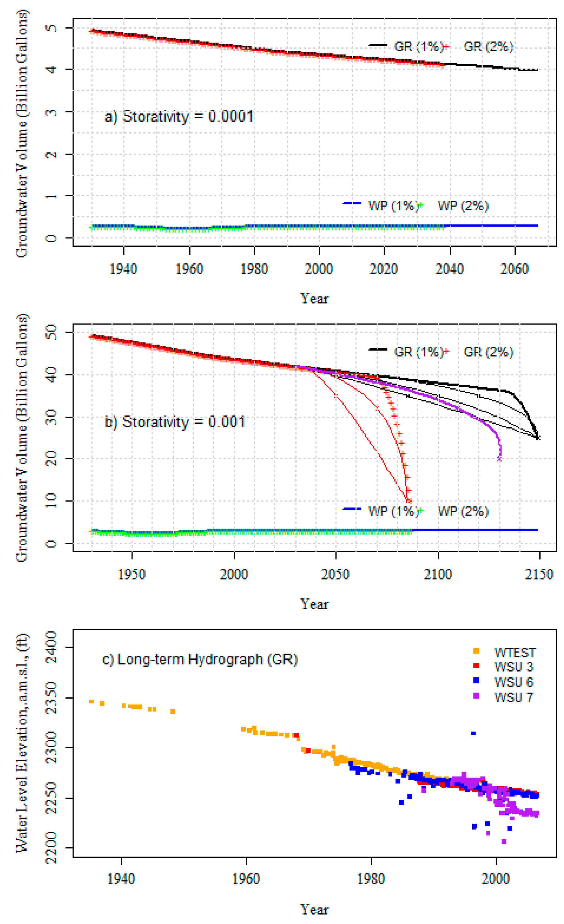
4.3. Simulation of Groundwater Volume of the Aquifers

Based on the water balance (Equations (1) to (9)), simulations were carried out to find the response of these aquifers. Figure 4a,b show the simulation results of groundwater storage change between 1930 and 2150 with storativity values of 0.0001 and 0.001, respectively. The population of the PB was validated in 2005 and 1%–2% increase in population was adopted after that. The percentage value in the parenthesis in the figure shows the applied population growth in the simulation. As expected, simulation result shows that the WP decreased until 1960s and reverts back its original level in the 1990s. After 1990s, the water level of WP is constant as the model considers no drawdown. The aquifer dynamics of upper WP may have little interest compared to the lower GR as it is fairly constant, but the entire recharge process to GR is dominated by WP. In the model, GR adopts a constant decline of 0.45 m/year until 1990s and after that, a decline about 0.3 m/year until the maximum allowed recharge reached, i.e., 4 cm/year. Figure 4a (smaller storativity value of 0.0001) shows the validity of these assumptions are until about 2070 and 2040 to 1% and 2% population growth, respectively. Because of the smaller storage capacity of GR, i.e., 5 billion gallons, it will not be able to fulfill the entire demand after these cut off points. These cutoff points do not imply that the groundwater cannot be further extracted, but probably only a portion of demand can fulfilled or alternative sources need be sought out to fulfill the entire demand. When a 2.5% population growth is applied, there was a significant decline in water level of GR after 2050 based on the analysis conducted by Beall [45].
In an optimistic scenario (with larger storativity i.e., 0.001), these assumptions can be valid until 2090 for 2% population growth and beyond 2150 to 1% population growth. The actual shape of these simulations might be less intuitive as we have adopted constant drawdown in the simulation, but looking back 100 years drawdown, this assumption can be acceptable for near future. Figure 4b shows the illustration of the curve fitting of aquifer decline if constant drawdown replaced by variable drawdown ( for 1%, 2% population growth or somewhat between all these simulations, purple line) assuming the cutoff points is reasonable. With a smaller storativity value, to maintain the current pumpage from GR, either larger groundwater regions or larger recharge rate is needed [62]. After analyzing the results (Figure 4a,b), it is not pragmatic to increase the population growth lager than 2%. Sensitivity analysis as well as the uncertainty analysis can be conducted altering numerous parameters of the aquifer (surface area, storativity, groundwater depth, recharge, population growth etc.), but we believe that the model had sufficiently captured the behavior of the aquifer with a range of applied storativity, variable recharge rate as well as surface area. Figure 4c shows the observed long-term monthly hydrograph of GR wells at Washington State University (WSU) and GR test well (WTEST).
Figure 5 shows the simulation results of the possible contribution of recharge to GR from WP in centimeters. Historical and current observations show that GR is declining nearly at the constant rate even though there is a significant surge in GR extraction (from 1930 −0.14 billion gallons to 2005 −2.5 billion gallons). Water balance indicates that the WP may receive a considerable water from the entire PB (up to 22 billion gallons/year) compared to the tiny amount of water extraction from WP (less than a billion gallons/year), but the current water level of WP is fairly constant. Similarly, the current pumpage from GR (>2 billion gallons) largely exceeds the observed drawdown (~0.02–0.09 billion gallons) which also suggests that the GR may be actively recharging. Figure 5 shows that the majority of the recharged water from WP is either departing or potentially unusable when there is less demand in GR. However, when the demand in GR increased, more water from WP is infiltrating to GR, indicating a variable recharge rate.
While discussing the recharge to GR, an important concern is how these estimated recharge values comply with the age dating of GR groundwater. As mentioned earlier, some of the studies dates water from GR as early as 30,000 years (BP). The answer might not be straightforward and probably the most up-to-date explanation can be considered to be the approach adopted by [45]. This study keeps on the paradigm that GR may be actively recharging based on the water balance model which is supported by some of the most current studies [61,62]. Figure 5 shows that with an increase of water demand in GR, recharge from WP to GR is also consistently increasing until it reaches the threshold. Figure 5a shows that after 2060, GR no more able to fulfill the entire water demand of PB for 1% population growth and even shorter period for 2% growth, which is an example of deficit threshold implied in the model. The maximum recharge value is about about 2 cm/year within these periods.
In an instance of a higher storativity with larger storage capacity (0.001, Figure 5b), the GR will be able to fulfill the entire water demand for 1% population growth until 2140 with the assumed constant drawdown. When the recharge from WP to GR reaches the recharge threshold (Figure 5a,b), there will be a sharp decline of groundwater beyond this point (drawdown is shown by the red line in secondary vertical-axis). Beall et al. [45] utilized the dual storage and resident time concept to understand the behavior of the GR aquifer. Results confirmed that in order to maintain the current trend of drawdown in the future, either more water from WP needs to enter in GR or GR will observe larger drawdown (red line at secondary axis) if recharge to GR is constrained by other hydrogeological conditions. As discussed earlier, it is difficult to predict the actual behavior and the possible trend of groundwater depletion in the future because it might be the function of a multiple parameters, but the larger overdraft of groundwater would obviously increase the drawdown.
In a separate simulation, we tested a hypothesis of no recharge to GR which makes the GR as a sole function of GR pumpage (Figure 6). If assumed no recharge to GR, water extraction from GR should be equal to drawdown of GR. Without an acceptable storativity value, we can argue the fruitfulness of this simulation, but it will help to distinguish the role of recharge. Simulation result shows that entire groundwater from GR should have been emptied in around the 2000s (with higher storativity 0.001, Figure 6), with the current applied drawdown (0.3 m/year) and 1% population growth. Analyzing this scenario, we attempted to increase life of GR by increasing surface area of GR assuming identical to the entire PB (2044 km2). This attempt does not help to increase the life of the GR because of the lack of continuous source to replenish the pumpage. This probably implies that a significant amount of water might be entering as recharge to GR to balance the deficit. In a recent study, Piersol and Sprenke [61] indicated that about 93.5% ± 2.6% of water in GR is contributed by the recharge which agrees the finding this study (Figure 7).
Figure 7 shows the contribution of recharge to GR as a percentage. It was computed based on the water that is extracted from the GR to recharged to GR. Results show that up to 96% of GR demand might had been fulfilled by the recharge between 1930 and 2005. In the future, more water is needed to fulfill the increased demand of GR to maintain the current decline rate of 0.3 m/year or GR will face a larger decline (Figure 4 and Figure 5). Figure 7b shows that the % contribution of recharge decreased when recharge value reached the threshold value, i.e., 4 cm/year.
Figure 8 shows the comparison among the different pumping entities and recharge to GR. The GR pumpage closely followed to the recharge to GR. It is because of the dependence of pumpage to recharge and it this will increase in the future as the demand increases. At the end of the simulation period i.e., at 2150, the demand of PB (combined WP and GR) will be about 10 billion gallons (1% growth).

5. Conclusions

A system dynamics approach facilitated to conduct analysis of the PB watershed and groundwater aquifers with various scenarios. This analysis assisted to estimate WP recharge from water balance and GR recharge via indirect estimation of drawdown. Even though, there were various uncertainties in the parameters (especially in storativity), this study helped to understand some critical future scenarios of PB aquifers. Our study demonstrated that about 90% of water extracted from GR may have been contributed from recharge and GR gets about 0–2 cm/year from recharge (until 2005). The estimated recharge to GR is in the reasonable range while compared to the published values. With this modeling approach, even in an optimistic scenario with larger storativity and larger GR surface area, the historical and current water level depletion may have not been sustained without recharge. Simulation results indicated that the GR will face consistent pressure in the coming years because of the increased growth and probably observe an abrupt decline once recharge threshold is reached. Because of the implied assumptions and parameter values ( with low storativity value), even if the simulation was carried out for longer period i.e., 150 years, the results showed that GR aquifer can face significant drawdown after 2050. As per the previous studies, this study also confirmed that the GR aquifer is at high risk and it is being exploited in an unsustainable way. However, equally, these results should be taken cautiously because various assumptions and constraints had been implied in the model. Our attempt here is rather utilizing the available data than validate the data. The major limitations of this study can be considered as how these estimated recharge values compare to the age dating of groundwater and applicability of the storativity values.

Acknowledgments

This study is financially supported by Water of West, University of Idaho at the period of 2006–2007. We want to acknowledge Erin Brooks, John Bush, and Jennifer Hinds for discussions of different subject matters of the project. We want to thank University of Idaho, Washington State University, and Palouse Basin Aquifer Committee for providing the data. We want to acknowledge Bibha Dhungana for proofreading and for the valuable suggestions. We want to thank the anonymous reviewers who helped to increase the quality of the manuscript.

Author Contributions

Ramesh Dhungel was responsible for analyzing the data and modeling with the system dynamics. Fritz Fielder conducted the surface water analysis from the gauging stations as well as providing the overall insight of the Palouse Basin Sustainability effort. All authors contributed with idea, writing and discussions.

Conflicts of Interest

The authors declare no conflict of interest.

References

  1. Konikow, L.F. Contribution of global groundwater depletion since 1900 to sea-level rise. Geophys. Res. Lett. 2011, 38, L17401. [Google Scholar] [CrossRef]
  2. Gleeson, T.; Alley, W.M.; Allen, D.M.; Sophocleous, M.A.; Zhou, Y.; Taniguchi, M.; VanderSteen, J. Towards Sustainable Groundwater Use: Setting Long-Term Goals, Backcasting, and Managing Adaptively. Ground Water 2012, 50, 19–26. [Google Scholar] [CrossRef] [PubMed]
  3. Shamsudduha, M.; Taylor, R.G.; Longuevergne, L. Monitoring groundwater storage changes in the highly seasonal humid tropics: Validation of GRACE measurements in the Bengal Basin. Water Resour. Res. 2012, 48, W02508. [Google Scholar] [CrossRef]
  4. Lund, J.; Harter, T. California’s Groundwater Problems and Prospects. Available online: https://californiawaterblog.com/2013/01/30/californias-groundwater-problems-and-prospects/ (accessed on 11 March 2016).
  5. Voss, K.A.; Famiglietti, J.S.; Lo, M.; de Linage, C.; Rodell, M.; Swenson, S.C. Groundwater depletion in the Middle East from GRACE with implications for transboundary water management in the Tigris-Euphrates-Western Iran region. Water Resour. Res. 2013, 49, 904–914. [Google Scholar] [CrossRef] [PubMed]
  6. Werner, A.D.; Zhang, Q.; Xue, L.; Smerdon, B.D.; Li, X.; Zhu, X.; Yu, L.; Li, L. An Initial Inventory and Indexation of Groundwater Mega-Depletion Cases. Water Resour. Manag. 2012, 27, 507–533. [Google Scholar] [CrossRef]
  7. Taylor, R.G.; Scanlon, B.; Döll, P.; Rodell, M.; van Beek, R.; Wada, Y.; Longuevergne, L.; Leblanc, M.; Famiglietti, J.S.; Edmunds, M.; et al. Ground water and climate change. Nat. Clim. Change 2013, 3, 322–329. [Google Scholar] [CrossRef] [Green Version]
  8. Shen, H.; Leblanc, M.; Tweed, S.; Liu, W. Groundwater depletion in the Hai River Basin, China, from in situ and GRACE observations. Hydrol. Sci. J. 2015, 60, 671–687. [Google Scholar] [CrossRef]
  9. Castle, S.L.; Thomas, B.F.; Reager, J.T.; Rodell, M.; Swenson, S.C.; Famiglietti, J.S. Groundwater depletion during drought threatens future water security of the Colorado River Basin. Geophys. Res. Lett. 2014, 41, 2014GL061055. [Google Scholar] [CrossRef] [PubMed]
  10. Konikow, L.F. Long-Term Groundwater Depletion in the United States. Groundwater 2015, 53, 2–9. [Google Scholar] [CrossRef] [PubMed]
  11. Richey, A.S.; Thomas, B.F.; Lo, M.-H.; Reager, J.T.; Famiglietti, J.S.; Voss, K.; Swenson, S.; Rodell, M. Quantifying renewable groundwater stress with GRACE. Water Resour. Res. 2015, 51, 5217–5238. [Google Scholar] [CrossRef] [PubMed]
  12. Scanlon, B.R.; Healy, R.W.; Cook, P.G. Choosing appropriate techniques for quantifying groundwater recharge. Hydrogeol. J. 2002, 10, 18–39. [Google Scholar] [CrossRef]
  13. Xu, Y.; Beekman, H.E. Review of Groundwater Recharge Estimation in Arid and Semi-Arid Southern Africa. 2003. Available online: http://unesdoc.unesco.org/images/0013/001324/132404e.pdf (accessed on 11 March 2016).
  14. Obuobie, E.; Diekkrueger, B.; Agyekum, W.; Agodzo, S. Groundwater level monitoring and recharge estimation in the White Volta River basin of Ghana. J. Afr. Earth Sci. 2012, 71–72, 80–86. [Google Scholar] [CrossRef]
  15. McMahon, P.B.; Plummer, L.N.; Böhlke, J.K.; Shapiro, S.D.; Hinkle, S.R. A comparison of recharge rates in aquifers of the United States based on groundwater-age data. Hydrogeol. J. 2011, 19, 779–800. [Google Scholar] [CrossRef]
  16. Tyler, S.W.; Chapman, J.B.; Conrad, S.H.; Hammermeister, D.P.; Blout, D.O.; Miller, J.J.; Sully, M.J.; Ginanni, J.M. Soil-water flux in the Southern Great Basin, United States: Temporal and spatial variations over the last 120,000 years. Water Resour. Res. 1996, 32, 1481–1499. [Google Scholar] [CrossRef]
  17. Wolock, D.M. Estimated Mean Annual Natural Groundwater Recharge in the Conterminous United States; U.S. Geological Survey: Reston, VA, USA, 2003.
  18. Scanlon, B.R.; Keese, K.E.; Flint, A.L.; Flint, L.E.; Gaye, C.B.; Edmunds, W.M.; Simmers, I. Global synthesis of groundwater recharge in semiarid and arid regions. Hydrol. Process. 2006, 20, 3335–3370. [Google Scholar] [CrossRef]
  19. Crosbie, R.; Jolly, I.D.; Leaney, F.W.J.; Petheram, C.; Wohling, D.; Commission, N.W. Review of Australian Groundwater Recharge Studies. CSIRO, 2010. Available online: http://www.clw.csiro.au/publications/waterforahealthycountry/2010/wfhc-review-Australian-recharge.pdf (accessed on 11 March 2016).
  20. McKenna, J.M. Water Use in the Palouse Basin. The Palouse Basin Aquifer Committee 2000 Annual report. , 2001. Available online: http://www.webpages.uidaho.edu/pbac/pubs/00report.pdf (accessed on 11 March 2016).
  21. Stevens, P.R. Ground-Water Problems in the Vicinity of Moscow, Latah County, Idaho: Idaho Waters Digital Library. Available online: http://digital.lib.uidaho.edu/cdm/ref/collection/idahowater/id/286 (accessed on 4 January 2016).
  22. Smoot, J.L.; Ralston, D.R. Hydrogeology and Mathematical Model of Ground Water Flow in the Pullman-Moscow Region, Washington And Idaho. Available online: http://digital.lib.uidaho.edu/cdm/ref/collection/idahowater/id/310 (accessed on 11 March 2016).
  23. Johnson, G.E. Estimating Groundwater Recharge Beneath Different Slope Positions in the Palouse formation Using a Numerical Unsaturated Flow Model. Master’s Thesis, Washington State University, Pullman, WA, USA, 1991. [Google Scholar]
  24. Muniz, H.R. Computer Modeling of Vadose. Zone Groundwater Flux at a Hazardous Waste Site; Washington State University: Pullman, WA, USA, 1991. [Google Scholar]
  25. O’Brien, R.; Keller, C.K.; Smith, J.L. Multiple Tracers of Shallow Ground-Water Flow and Recharge in Hilly Loess. Groundwater 1996, 34, 675–682. [Google Scholar] [CrossRef]
  26. Lum, W.E.; Smoot, J.L.; Ralston, D.R. Geohydrology and Numerical Model Analysis of Ground-Water Flow in the Pullman-Moscow area, Washington and Idaho. Water-Resources Investigations Report. Available online: https://pubs.er.usgs.gov/publication/wri894103 (accessed on 11 March 2016).
  27. O’Geen, A.T. Assessment of Hydrologic Processes Across Multiple Scales in Soils/Paleosol Sequences Using Environmental Tracers: Idaho Waters Digital Library. Available online: http://digital.lib.uidaho.edu/cdm/ref/collection/idahowater/id/333 (accessed on 4 January 2016).
  28. Larson, K.R.; Keller, C.K.; Larson, P.B.; Allen-King, R.M. Water resource implications of 18O and 2H distributions in a basalt aquifer system. Groundwater 2000, 38, 947–953. [Google Scholar] [CrossRef]
  29. Dhungel, R. Water Resource Sustainability of the Palouse Region: A Systems Approach; University of Idaho: Moscow, ID, USA, 2007. [Google Scholar]
  30. Reeves, M. Estimating Recharge Uncertainty Using Bayesian Model. Averaging and Expert Elicitation with Social Implications; University of Idaho: Moscow, ID, USA, 2009. [Google Scholar]
  31. Dijksma, R.; Brooks, E.S.; Boll, J. Groundwater recharge in Pleistocene sediments overlying basalt aquifers in the Palouse Basin, USA: Modeling of distributed recharge potential and identification of water pathways. Hydrogeol. J. 2011, 19, 489–500. [Google Scholar] [CrossRef]
  32. Crosby, J.W. Water Dating Techniques as Applied to the Pullman-Moscow Ground-Water Basin; Technical Extension Service, Washington State University: Pullman, WA, USA, 1965. [Google Scholar]
  33. Foxworthy, B.L.; Washburn, R.L. Ground Water in the Pullman Area, Whitman County, Washington. Water Supply Paper. Available online: http://pubs.usgs.gov/wsp/1655/report.pdf (accessed on 11 March 2016).
  34. Barker, R.A. Computer Simulation and Geohydrology of a Basalt Aquifer System in the Pullman-Moscow Basin, Washington and Idaho; Stanford University: Stanford, CA, USA, 1979. [Google Scholar]
  35. Hydrogeology and a Mathematical Model of Ground-Water Flow in the Pullman-Moscow Region, Washington and Idaho: Idaho Waters Digital Library. Available online: http://digital.lib.uidaho.edu/cdm/ref/collection/idahowater/id/310 (accessed on 4 January 2016).
  36. Porter, D.E. Industrial Dynamics. Jay Forrester. M.I.T. Press, Cambridge, Mass.; Wiley, New York, 1961. xv + 464 pp. Illus. $18. Science 1962, 135, 426–427. [Google Scholar] [CrossRef]
  37. Stephenson, K. The What and Why of Shared Vision Planning for Water Supply 2000. Available online: http://www.sharedvisionplanning.us/docs/WaterSecurity03Stephenson.pdf (accessed on 11 March 2016).
  38. Palmer, R.N.; Keyes, A.M.; Fisher, S. Empowering stakeholders through simulation in water resources planning. In Proceedings of the 20th Anniversary Conference: Water Management in the ’90s. A Time for Innovation, Seattle, WA, USA, 1–5 May 1993.
  39. Simonovic, S.P.; Fahmy, H.; El-Shorbagy, A. The Use of Object-Oriented Modeling for Water Resources Planning in Egypt. Water Resour. Manag. 1997, 11, 243–261. [Google Scholar] [CrossRef]
  40. Xu, Z.X.; Takeuchi, K.; Ishidaira, H.; Zhang, X.W. Sustainability Analysis for Yellow River Water Resources Using the System Dynamics Approach. Water Resour. Manag. 2002, 16, 239–261. [Google Scholar] [CrossRef]
  41. Spatial System Dynamics: New Approach for Simulation of Water Resources Systems. J. Comput. Civ. Eng. 2004, 18, 331–340.
  42. Tidwell, V.C.; Passell, H.D.; Conrad, S.H.; Thomas, R.P. System dynamics modeling for community-based water planning: Application to the Middle Rio Grande. Aquat. Sci. 2004, 66, 357–372. [Google Scholar] [CrossRef]
  43. Sehlke, G.; Jacobson, J. System dynamics modeling of transboundary systems: The bear river basin model. Ground Water 2005, 43, 722–730. [Google Scholar] [CrossRef] [PubMed]
  44. Winz, I.; Brierley, G.; Trowsdale, S. The Use of System Dynamics Simulation in Water Resources Management. Water Resour. Manag. 2008, 23, 1301–1323. [Google Scholar] [CrossRef]
  45. Beall, A.; Fiedler, F.; Boll, J.; Cosens, B. Sustainable Water Resource Management and Participatory System Dynamics. Case Study: Developing the Palouse Basin Participatory Model. Sustainability 2011, 3, 720–742. [Google Scholar] [CrossRef]
  46. Ryu, J.H.; Contor, B.; Johnson, G.; Allen, R.; Tracy, J. System Dynamics to Sustainable Water Resources Management in the Eastern Snake Plain Aquifer Under Water Supply Uncertainty1. J. Am. Water Resour. Assoc. 2012, 48, 1204–1220. [Google Scholar] [CrossRef]
  47. Hoekema, D.J.; Sridhar, V. A System Dynamics Model for Conjunctive Management of Water Resources in the Snake River Basin. J. Am. Water Resour. Assoc. 2013, 49, 1327–1350. [Google Scholar] [CrossRef]
  48. Dhungel, R.; Fiedler, F. Price Elasticity of Water Demand in a Small College Town: An Inclusion of System Dynamics Approach for Water Demand Forecast. Air Soil Water Res. 2014, 7, 77–91. [Google Scholar] [CrossRef]
  49. Fernald, A.; Tidwell, V.; Rivera, J.; Rodríguez, S.; Guldan, S.; Steele, C.; Ochoa, C.; Hurd, B.; Ortiz, M.; Boykin, K.; et al. Modeling Sustainability of Water, Environment, Livelihood, and Culture in Traditional Irrigation Communities and Their Linked Watersheds. Sustainability 2012, 4, 2998–3022. [Google Scholar] [CrossRef]
  50. Roach, J.; Tidwell, V. A compartmental-spatial system dynamics approach to ground water modeling. Ground Water 2009, 47, 686–698. [Google Scholar] [CrossRef] [PubMed]
  51. Balali, H.; Viaggi, D. Applying a System Dynamics Approach for Modeling Groundwater Dynamics to Depletion under Different Economical and Climate Change Scenarios. Water 2015, 7, 5258–5271. [Google Scholar] [CrossRef]
  52. Niazi, A.; Prasher, S.O.; Adamowski, J.; Gleeson, T. A System Dynamics Model to Conserve Arid Region Water Resources through Aquifer Storage and Recovery in Conjunction with a Dam. Water 2014, 6, 2300–2321. [Google Scholar] [CrossRef]
  53. Mirchi, A.; Madani, K.; Watkins, D., Jr.; Ahmad, S. Synthesis of System Dynamics Tools for Holistic Conceptualization of Water Resources Problems. Water Resour. Manag. 2012, 26, 2421–2442. [Google Scholar] [CrossRef]
  54. 2002-2005 Palouse Ground Water Basin Water Use Report, Palouse Basin Aquifer Committee 2005. Available online: http://www.webpages.uidaho.edu/pbac/Annual_Report/Final_PBAC_Annual_Report_2002_2005_low_res.pdf (accessed on 11 March 2016).
  55. Water Matter in the City of Moscow, 10th Annual Palouse Basin Water Summit. Available online: https://www.ci.moscow.id.us/records/Publications/Fall14_Draft14_FinalWebRes.pdf (accessed on 11 March 2016).
  56. Ground Water Mangement Plan Pullman-Moscow Water Resources Committte, 1992. Available online: https://www.idwr.idaho.gov/waterboard/WaterPlanning/CAMP/RP_CAMP/PDF/2010/05-07-10_GW-MngmntPlan.pdf (accessed on 11 March 2016).
  57. Bush, J.; Hinds, J. Geologic overview of the Palouse Basin. In Presented at the Palouse Basin Water Summit, Moscow, ID, USA, 2006.
  58. Leek, F. Hydrogeological Characterization of the Palouse Basin Basalt Aquifer System, Washington and Idaho; Washington State University: Pullman, WA, USA, 2006. [Google Scholar]
  59. Douglas, A.A.; Osiensky, J.L.; Keller, C.K. Carbon-14 dating of ground water in the Palouse Basin of the Columbia river basalts. J. Hydrol. 2007, 334, 502–512. [Google Scholar] [CrossRef]
  60. Osiensky, J.L. The do’s and dont’s in current understanding of the Palouse Basin Grande Ronde 459 Aquifer system. In Presented at the Palouse Basin Water Summit, Moscow, ID, USA, 2006.
  61. Piersol, M.W.; Sprenke, K.F. A Columbia River Basalt Group Aquifer in Sustained Drought: Insight from Geophysical Methods. Resources 2015, 4, 577–596. [Google Scholar] [CrossRef]
  62. Moran, K. Interpretation of Long-Term Grande Ronde Aquifer Testing in the Palouse Basin of Idaho and Washington; University of Idaho: Moscow, ID, USA, 2011. [Google Scholar]
  63. Bennett, B. Recharge Implications of Strategic Pumping of the Wanapum. Aquifer System in the Moscow Sub-Basin; University of Idaho: Moscow, ID, USA, 2009. [Google Scholar]
  64. PRISM Climate Group. Oregon State University. Available online: http://prism.oregonstate.edu (accessed on 11 March 2016).
  65. Rushton, K.R.; Ward, C. The estimation of groundwater recharge. J. Hydrol. 1979, 41, 345–361. [Google Scholar] [CrossRef]
  66. Flerchinger, G.; Cooley, K. A ten-year water balance of a mountainous semi-arid watershed. J. Hydrol. 2000, 237, 86–99. [Google Scholar] [CrossRef]
  67. Everson, C.S. The water balance of a first order catchment in the montane grasslands of South Africa. J. Hydrol. 2001, 241, 110–123. [Google Scholar] [CrossRef]
  68. Estimating Groundwater Recharge. Available online: http://www.cambridge.org/us/academic/subjects/earth-and-environmental-science/hydrology-hydrogeology-and-water-resources/estimating-groundwater-recharge (accessed on 4 January 2016).
  69. Scanlon, B.R.; Dutton, A.R.; Sophocleous, M.A. Groundwater Recharge in Texas; Bureau of Economic Geology, University of Texas at Austin: Austin, TX, USA, 2002. [Google Scholar]
  70. Risser, D.W.; Gburek, W.J.; Folmar, G.J. Comparison of Methods for Estimating Ground-Water Recharge and Base Flow at a Small Watershed underlain by Fractured Bedrock in the Eastern United States; Scientific Investigations Report; 2005. Available online: http://pubs.usgs.gov/sir/2005/5038/pdf/sir2005-5038.pdf (accessed on 11 March 2016).
  71. Lee, C.-H.; Chen, W.-P.; Lee, R.-H. Estimation of groundwater recharge using water balance coupled with base-flow-record estimation and stable-base-flow analysis. Environ. Geol. 2006, 51, 73–82. [Google Scholar] [CrossRef]
  72. Estimation of Natural Groundwater Recharge; Simmers, I. (Ed.) Springer: Dordrecht, The Netherlands, 1988.
  73. Nimmo, J.R.; Healy, R.W.; Stonestrom, D.A. Aquifer Recharge. In Encyclopedia of Hydrological Sciences; John Wiley & Sons, Ltd.: New York, NY, USA, 2006. [Google Scholar]
  74. Thornthwaite, C.W.; Mather, J.R. Instructions and Tables for Computing Potential Evapotranspiration and the Water Balance; Laboratory of Climatology: Centerton, NJ, USA, 1957. [Google Scholar]
  75. Hargreaves, G.H. Estimation of Potential and Crop Evapotranspiration. Trans. ASAE 1974. [Google Scholar] [CrossRef]
  76. Sharda, V.N.; Kurothe, R.S.; Sena, D.R.; Pande, V.C.; Tiwari, S.P. Estimation of groundwater recharge from water storage structures in a semi-arid climate of India. J. Hydrol. 2006, 329, 224–243. [Google Scholar] [CrossRef]
  77. Hydrologic Conditions in the Palouse Aquifer. Available online: http://www.powershow.com/view/39753-ODYzN/Hydrologic_Conditions_in_the_Palouse_Aquifer_powerpoint_ppt_presentation (accessed on 4 January 2016).
  78. STELLA Research Technical Documentation; High Performance Systems, Inc.: Lebanon, NH, USA, 1996.
  79. Baines, C.A. Determination of Sustained Yield for the Shallow Basalt Aquifer in the Moscow Area, Idaho; Idaho Water Resources Research Institute: Moscow, ID, USA, 1992. [Google Scholar]
  80. Bauer, H.H.; Vaccaro, J.J. Estimates of Ground-Water Recharge to the Columbia Plateau Regional Aquifer System, Washington, Oregon, and Idaho, for Predevelopment and Current Land-Use Conditions; Water-Resources Investigations Report; U.S. Geological Survey; Books and Open-File Reports Section; 1990. Available online: http://pubs.usgs.gov/wri/1988/4108/report.pdf (accessed on 11 March 2016).
Figure 1. Location map of Palouse Basin watershed and surface water and groundwater regions.
Hydrology 03 00013 g001
Figure 2. (a) Conceptual schematic of the Palouse Basin Watershed, water-balance based on the variable surface areas and pumping entities (left) (b) Water balance based on the surface area identical to the Palouse Basin (right).
Hydrology 03 00013 g002
Figure 3. (a) Palouse Basin groundwater causal loop diagram in a simplest form; (b) Major components of System Dynamics model of the Palouse Basin watershed.
Hydrology 03 00013 g003
Figure 4. Simulation results of volume of water in (a) Wanapum and Grand Ronde (billion gallons—storativity −0.0001) (b) curve fitting of drawdown (black for 1% growth, red for 2% growth and purple for some hypothetical midway between 1% and 2%—storativity −0.001) (c) obseved long-term GR hydrograph at Washington State University (WSU) GR Wells (above mean seal level (a.m.s.l.)).
Hydrology 03 00013 g004
Figure 5. Simulation results of estimated recharge to Grand Ronde and applied drawdown values (cm).
Hydrology 03 00013 g005
Figure 6. Simulation result of the volume of water in Wanapum and Grande in a billion gallons (1% population growth) assuming no recharge to Grand Ronde.
Hydrology 03 00013 g006
Figure 7. Simulation result of percent contribution of WP to GR as recharge.
Hydrology 03 00013 g007
Figure 8. Simulation result of recharge to Grand Ronde (GR), GR pumpage, WP pumpage and total Pumpage (1% population growth).
Hydrology 03 00013 g008
Table 1. Period of Availability of Daily Discharge of USGS Gauging Stations of Palouse Basin.
Stations (Y)Site NameStations Used for Filling Gaps (X)Linear Regression EquationPeriod of Availability
13349210Entire Basin13345000y = 1.3951x + 22.83,
R2 = 0.8916
10/01/1963-09/30/1995
13345300Palouse River at Palouse, WA13345000y = 1.0381x + 1.54,
R2 = 0.9708
04/19/1973–10/02/1980
13346100Palouse River at Colfax, WA (North Fork)13345000y = 1.0798x + 13.60,
R2 = 0.9352
10/01/1963–05/31/1979
13346800Paradise Creek at UI at Moscow, ID13348000y = 0.2032x − 0.29,
R2 = 0.719
10/01/1978–09/30/2006
13348000South Fork Palouse river at Pullman, WA13346800y = 3.5385x + 10.11,
R2 = 0.719
02/01/1934–09/30/2006
Table 2. Mean Areal Recharge of Palouse Basin Sub-Watersheds (1971–2000).
Site NameUSGS Gauging StationsPrecipitationEvapotranspirationRunoffRecharge
(cm)(cm)(cm)(cm)
PEQsR
Entire Basin1334921070.949.017.24.7
Palouse River at Colfax, WA (North Fork)1334610059.345.27.76.4
South Fork above Colfax, WA (local)N/A58.944.810.43.7
Palouse River near Potlatch, ID1334500084.753.829.21.7
Palouse River at Palouse, WA1334530066.746.64.915.2
Paradise Creek at University of Idaho at Moscow, ID1334680075.149.816.48.9
South Fork Palouse River at Pullman, WA1334800066.146.710.29.2
Table 3. Estimated Recharge Rates of Wanapum Groundwater Aquifer ([29,30]).
SNNameMethodRecharge Rate
(cm·year−1)
1Stevens [21]Mass-balance3.0
2Johnson [23]One dimensional infiltration model (LEACHM)10.5
3Muniz [24]One dimensional infiltration model (LEACHM)2.5 to 10.3
4O’ Brien and Others [25]Chloride mass-balance0.2 to 2
5O’Geen [27]Chloride mass-balance0.3–1
6Foxworthy and Washburn [33]Mass-balance1.6
8Barker [34]Darcy’s Law1.70
9Reeves [30]Storage equation12.19
10Baines [79]Hill method and zero change method4.5
11Bauer and Vaccaro [80]USGS Daily Deep Percolation Model3.8
Table 4. Initial Volume of Groundwater in Aquifers.
NameGroundwater AreaStorativityAverage Thickness of AquifersTotal Groundwater Volume
(Total Depth)
(km2)(m)(Billion gallons)
WanapumSAV
Moscow81.7510−4137.190.29
Total0.29
Grande Ronde
Moscow63.9410−42710.45
Pullman235.9710−43051.90
Viola21.2510−42440.14
Palouse74.3210−41520.29
Colfax332.13 2442.14
Total728 Total4.94

