
Impact of Climate Change on Groundwater Resources in the Klela Basin, Southern Mali


Abstract
:1. Introduction
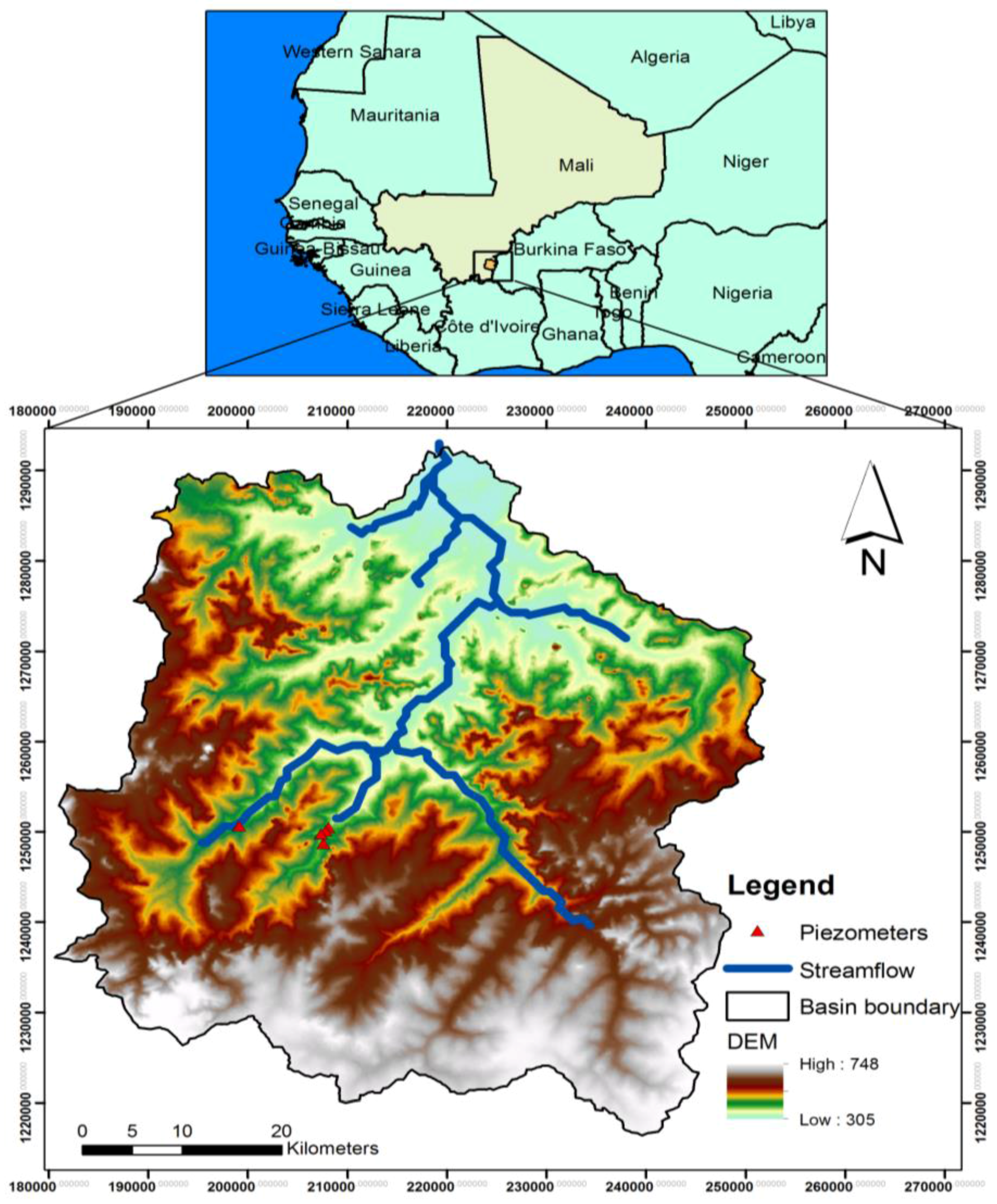
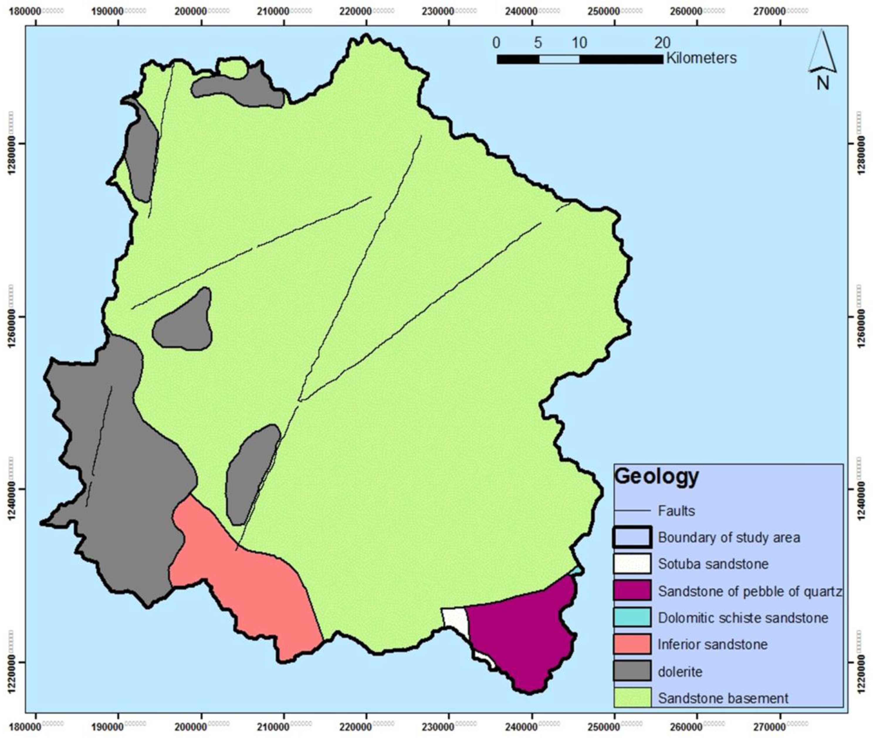
Study Area
2. Methodology
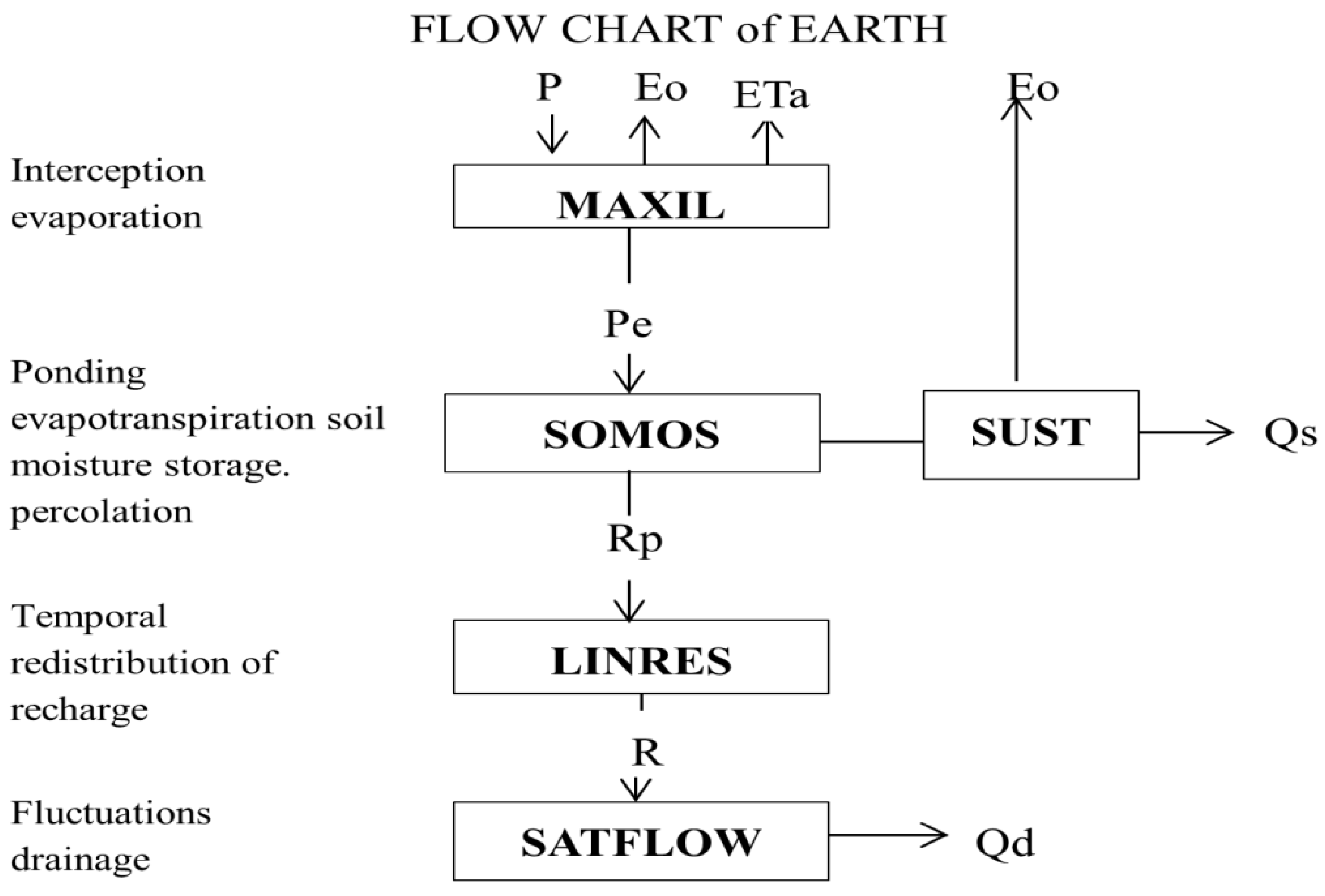
2.1. EARTH Model
- MAXIL (Maximal Interception Loss) estimates the water intercepted by the Earth`s surface.
- SOMOS (Soil Moisture Storage) describes water storage in the root zone and calculates changes in soil moisture storage by removing actual evapotranspiration, percolation, evaporation and surface runoff to determine the infiltrated precipitation.
- SUST (Surface Storage) calculates ponding and runoff. It uses SUSTmax, which is the maximum ponding volume that can be stored at the surface. If the amount of ponding is greater than SUSTmax, then runoff occurs.
- LINRES (Linear Reservoir Routing) redistributes percolation (output of SOMOS) over time in the unsaturated hard rock or soil beneath the root zone using the parametric transfer function.
- SATFLOW (Saturated Flow) is the last part of the EARTH model. It is a simple one-dimensional parametric model that uses the outputs from the previous modules. SATFLOW calculates the groundwater level using the recharge estimated by the direct part of the model.
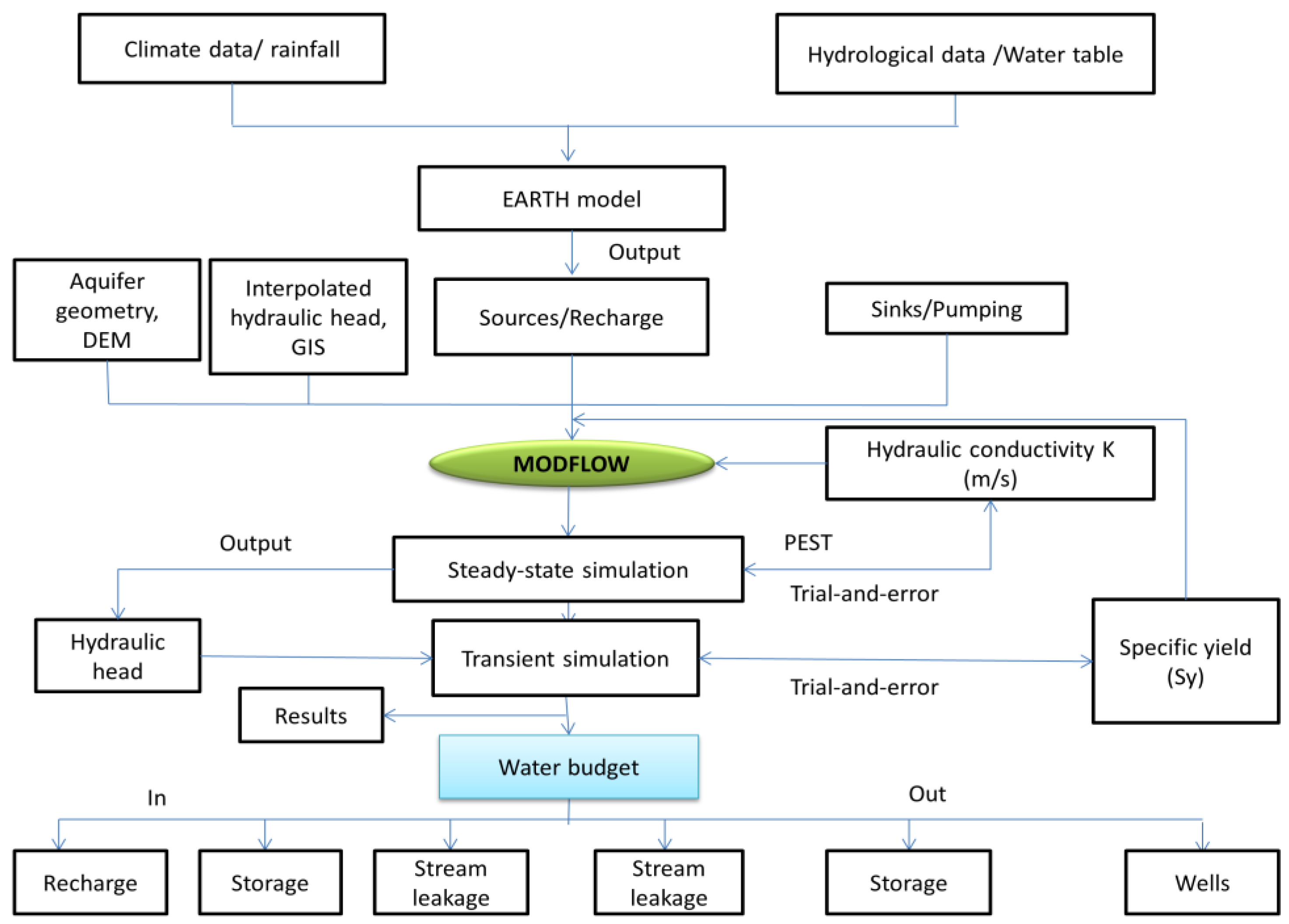
2.2. Groundwater Model
2.2.1. Spatial Discretization
2.2.2. Aquifer Geometry
2.2.3. Aquifer Properties
2.2.4. Boundary Conditions
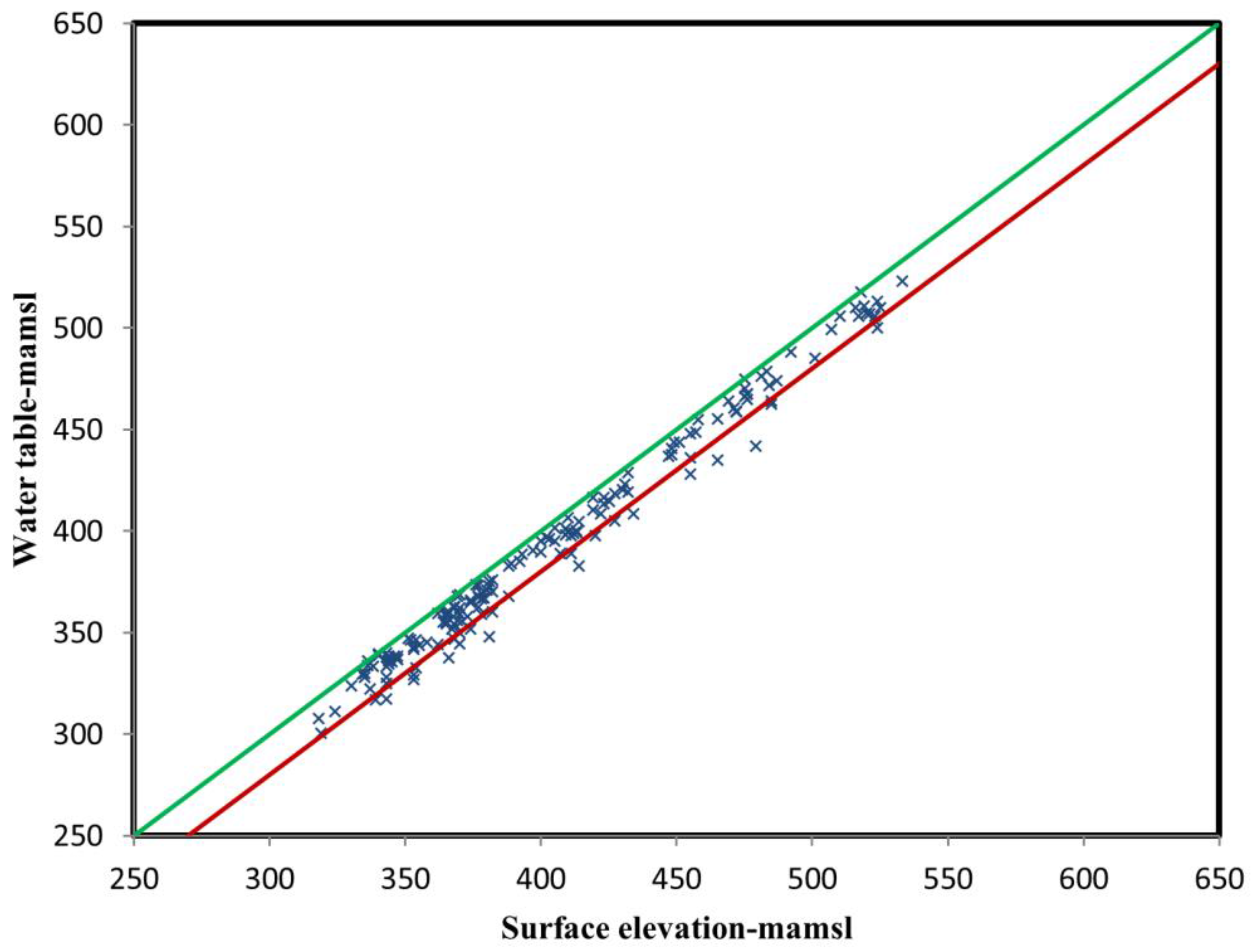
2.2.5. Initial Hydraulic Head
2.2.6. Groundwater Sources/Sinks
2.2.7. Streamflow Routing
3. Results and Discussion
3.1. EARTH Model
3.2. MODFLOW
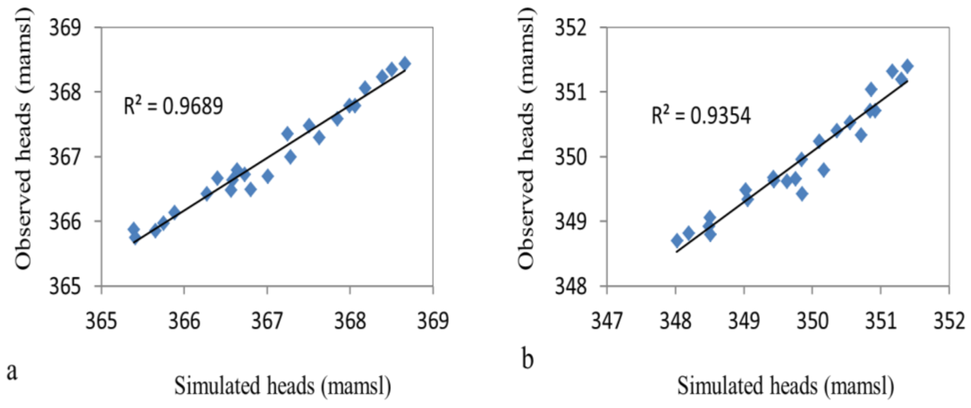
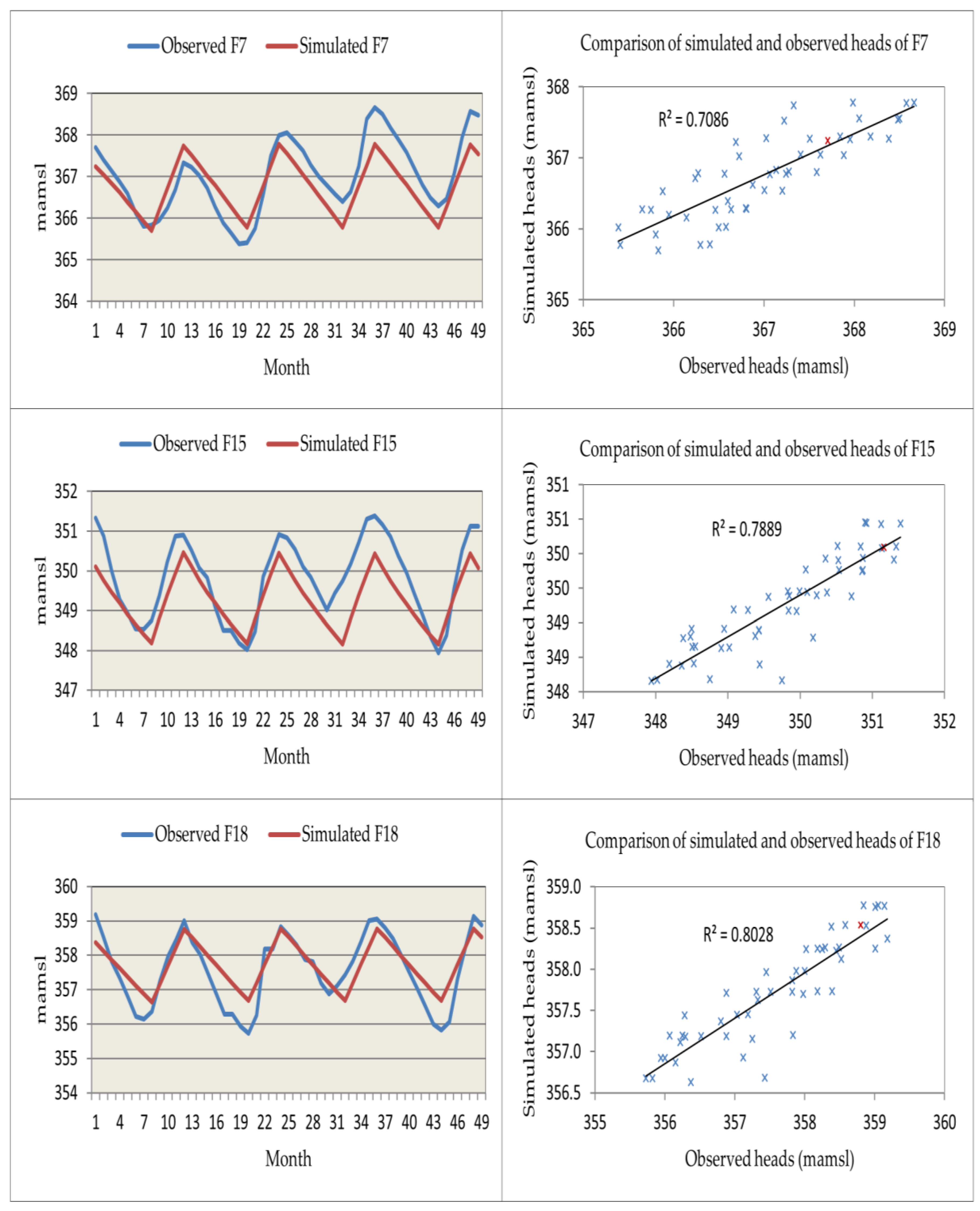
3.2.1. Calibration
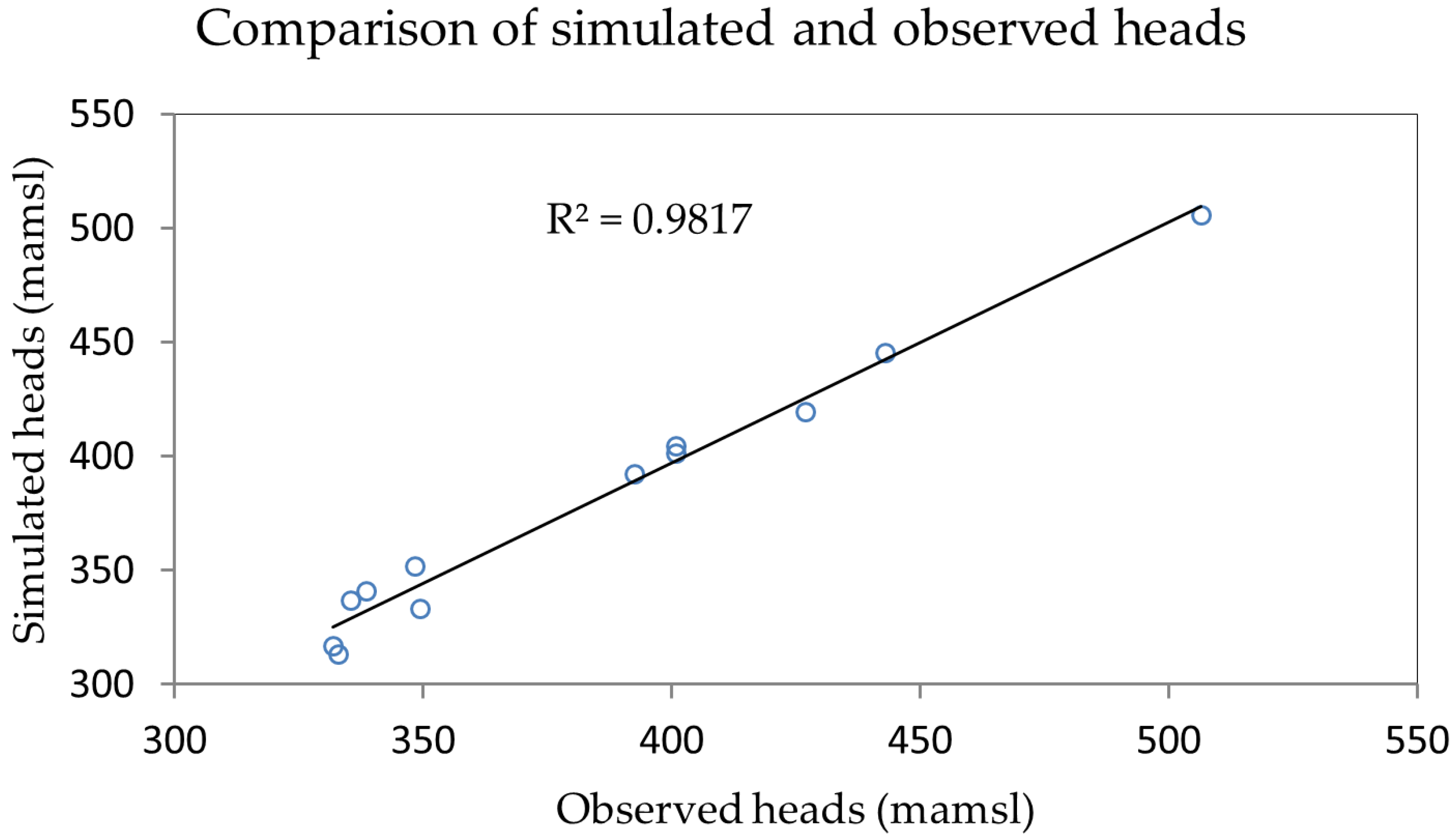
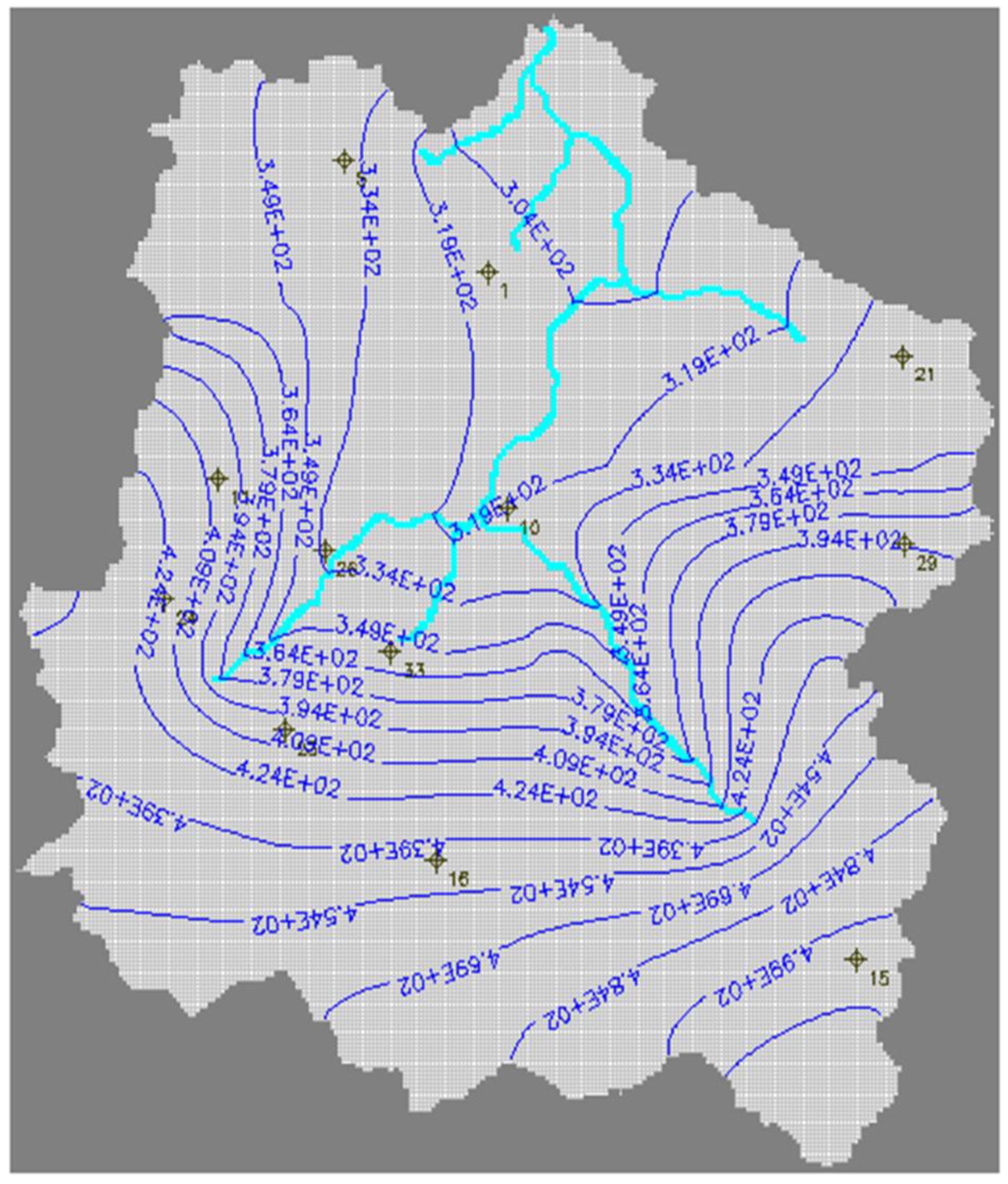
3.2.2. Steady-State Simulation
3.2.3. Transient Simulation
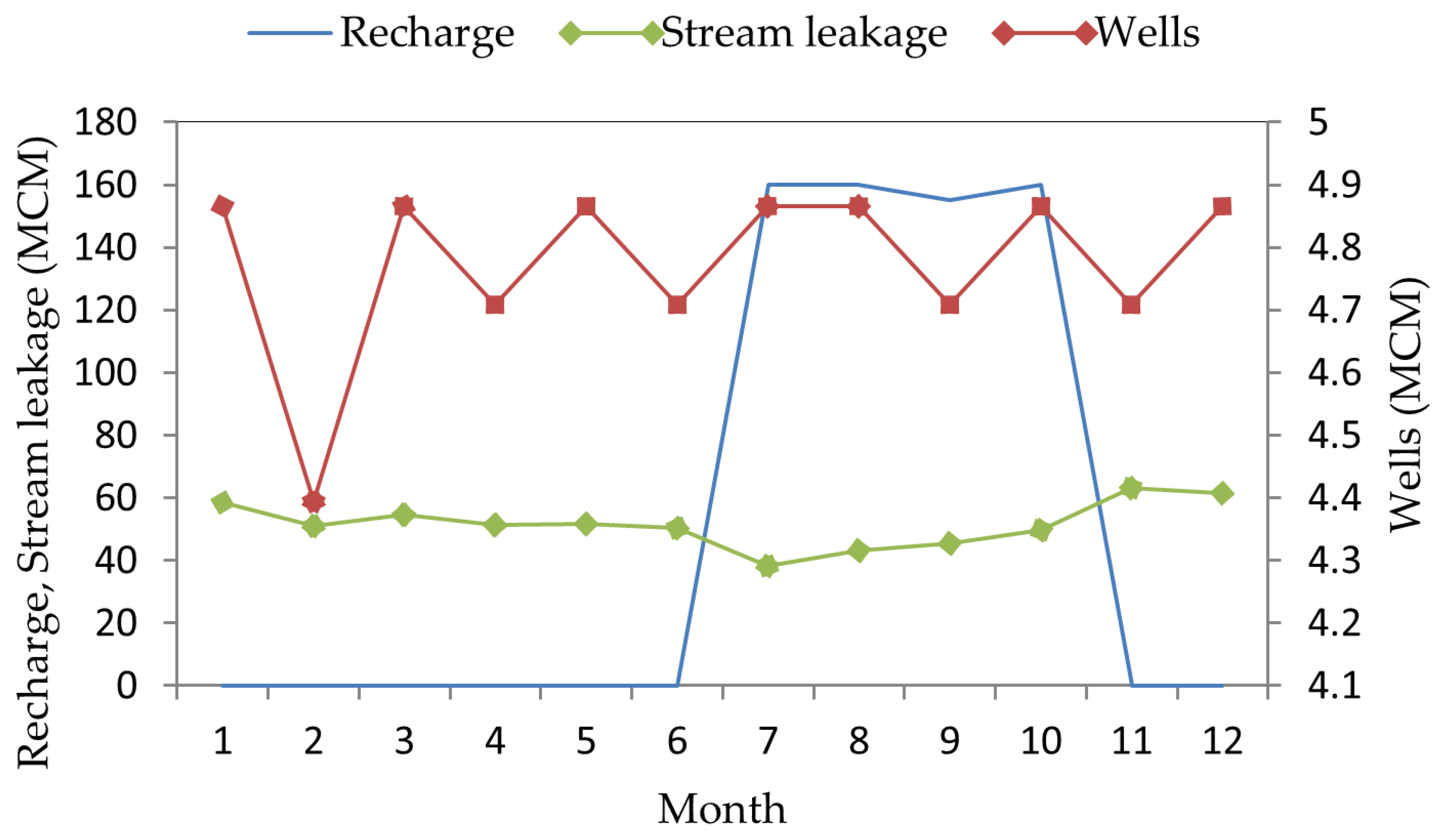
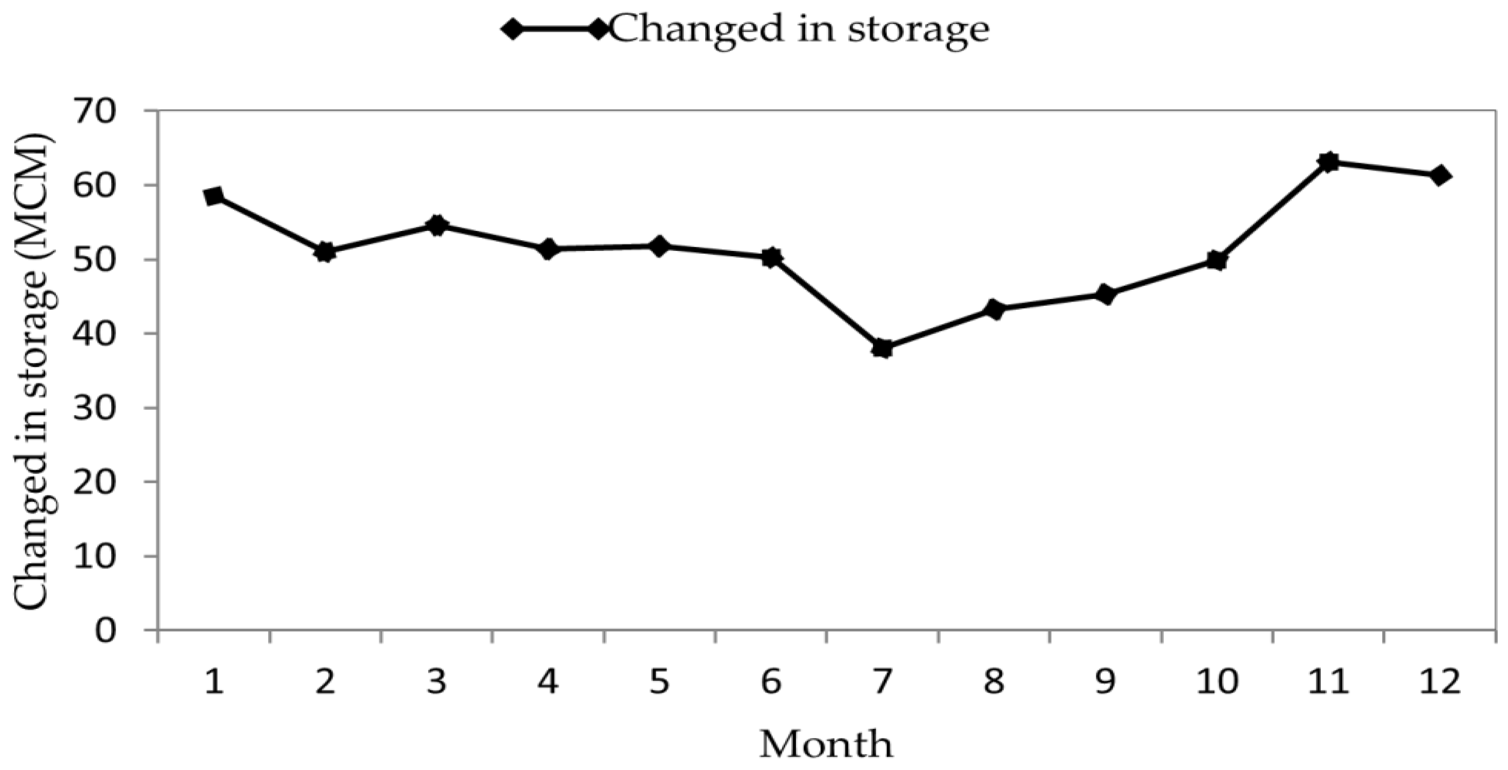
3.2.4. Water Budget
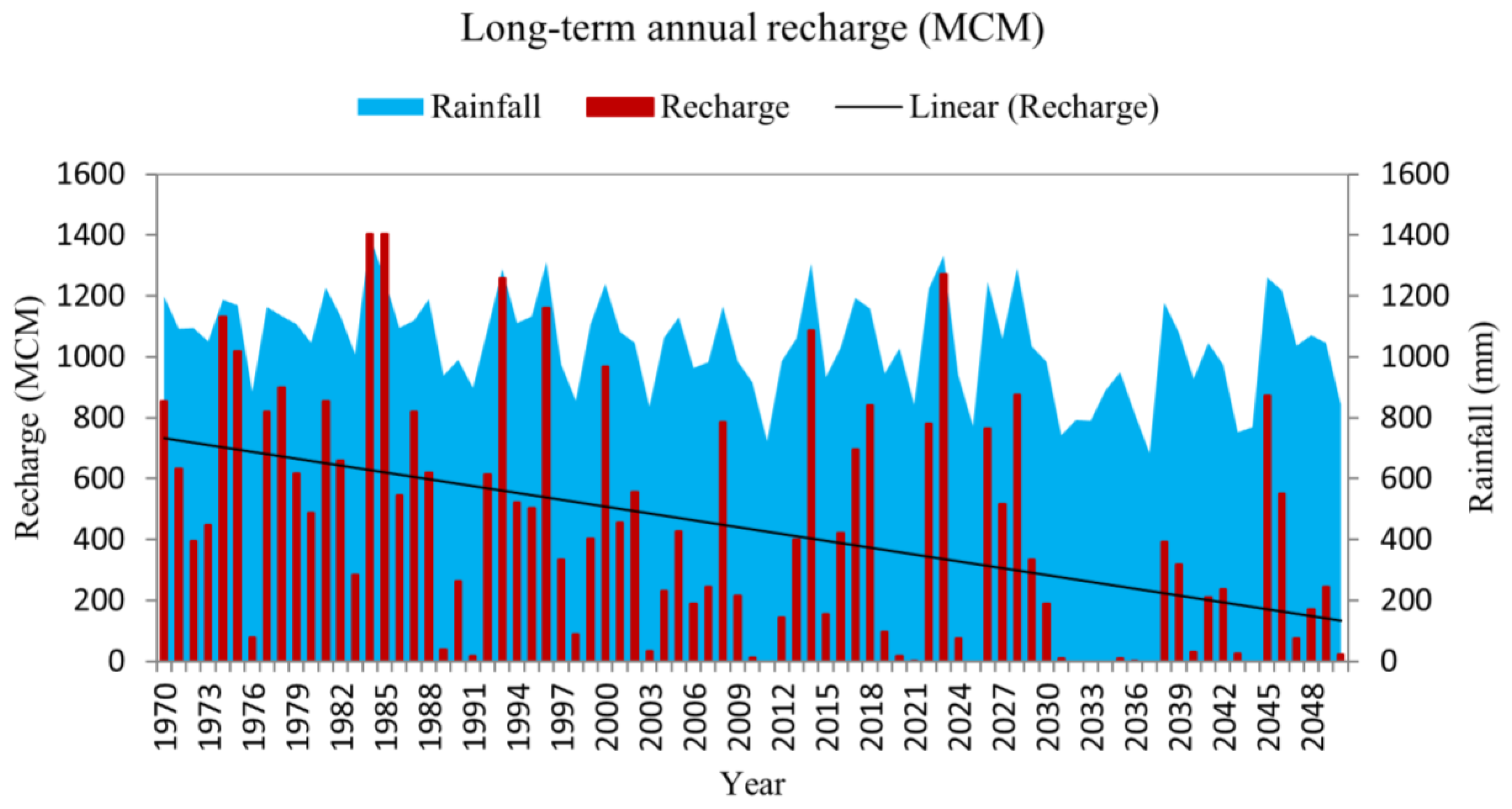
3.2.5. Scenario Quantification
4. Conclusions and Recommendations
Acknowledgments
Author Contributions
Conflicts of Interest
References
- McDonald, M.G.; Harbaugh, A.W. A modular three-dimensional finite-difference groundwater flow model. In Techniques of Water-Resources Investigations; Book 6, Chapter A1; U.S. Geological Survey: Reston, VA, USA, 1988; p. 586. [Google Scholar]
- Council, G.W. A Lake Package for MODFLOW (LAK2), Documentation and User’s Manual Version 2.2; HSI GEOTRANS, A Tetra Tech Company: Pasadena, CA, USA, 1999. [Google Scholar]
- AL-Fatlawi, A.N. The application of the mathematical model (MODFLOW) to simulate the behavior of groundwater flow in Umm Er Radhuma unconfined aquifer. Euphrates J. Agric. Sci. 2011, 3, 1–16. [Google Scholar]
- Saatsaz, M.; Chitsazan, M.; Eslamian, S.; Sulaiman, W.N.A. The application of groundwater modelling to simulate the behaviour of groundwater resources in the Ramhormooz Aquifer, Iran. Int. J. Water 2011, 6, 29–42. [Google Scholar] [CrossRef]
- Valerio, A.M. Modeling Groundwater-Surface Water Interactions in an Operational Setting by Linking Riverware with MODFLOW. Ph.D. Thesis, University of Colorado, Fort Collins, CO, USA, 2008. [Google Scholar]
- Banning, R.O.B. Analysis of the Groundwater/Surface Water Interactions in the Arikaree River Basin of Eastern Colorado. Ph.D. Thesis, Colorado State University, Fort Collins, CO, USA, 2010. [Google Scholar]
- Sehatzadeh, M. Groundwater Modelling in the Chikwawa district, lower Shire area of southern Malawi. Master’s Thesis, University of Oslo, Oslo, Norway, 2011. [Google Scholar]
- Taylor, C.M.; Lambin, E.F.; Stephenne, N.; Harding, R.J.; Essery, R.L.H. The Influence of Land Use Change on Climate in the Sahel. J. Clim. 2002, 15, 3615–3629. [Google Scholar] [CrossRef]
- Funk, C.; Rowland, J.; Adoum, A.; Eilerts, G.; White, L. A Climate Trend Analysis of Mali. Available online: http://pubs.usgs.gov/fs/2012/3105/fs2012-3105.pdf (accessed on 27 November 2015).
- Bricquet, J.P.; Bamba, F.; Mahe, G.; Toure, M.; Olivry, J.C. Évolution récente des ressources en eau de l’Afrique atlantique. Rev Sci Eau. 1997. (In French) [Google Scholar] [CrossRef]
- Bokar, H.; Mariko, A.; Bamba, F.; Diallo, D.; Kamagaté, B.; Dao, A. Impact Of Climate Variability On Groundwater Resources in Kolondieba Catchment Basin, Sudanese Climate Zone in Mali. Int. J. Eng. Res. Appl. 2012, 2, 1201–1210. [Google Scholar]
- Mahe, G. Surface/groundwater interactions in the Bani and Nakambe rivers, tributaries of the Niger and Volta basins, West Africa. Hydrol. Sci. J. 2009, 54, 704–712. [Google Scholar] [CrossRef]
- Mahé, G.; Olivry, J.C.; Dessouassi, R.; Orange, D.; Bamba, F.; Servat, E. Relations eaux de surface-eaux souterraines d’une rivière tropicale au Mali. Sci Terre Planetes. 2000, 330, 689–692. (In French) [Google Scholar] [CrossRef]
- WWAP. Rapport national sur la mise en valeur des ressources en eau: Mali. 2006. Available online: http://unesdoc.unesco.org/images/0014/001472/147267f.pdf (accessed on 27 November 2015). (In French)
- Chiang, W.-H.; Kinzelbach, W. Processing Modflow A Simulation System for Modeling Groundwater Flow and Pollution. 1998. Available online: https://www.researchgate.net/publication/238774706_Processing_MODFLOWa_Simulation_System_for_Modelling_Groundwater_Flow_and_Pollution (accessed on 27 November 2015).
- USAID. Plan de sécurité alimentaire commune rurale de Klela. 2006. Available online: http://fsg.afre.msu.edu/mali_fd_strtgy/plans/sikasso/sikasso/psa_klela.pdf (accessed on 27 November 2015). (In French)
- Direction Nationale de la Meteorologie du Mali. Departement de gestion des donnees. 2014. Available online: http://www.linguee.com/french-english/translation/direction+nationale+de+la+m%C3%A9t%C3%A9orologie.html (accessed on 27 November 2015). (In French)
- Direction Nationale de l`Hydraulique du Mali. Projet Mali Sud II. Bibliotheque. 1987. Available online: http://documentation.2ie-edu.org/cdi2ie/opac_css/index.php?lvl=notice_display&id=15175 (accessed on 27 November 2015). (In French)
- Van der Lee, J.; Gehrels, J. Modeling Aquifer Recharge, Introduction to Lumped Parameter Model EARTH; Hydrological Report; Free University of Amsterdam: Amsterdam, The Netherlands, 1990. [Google Scholar]
- Nyende, J. Application of isotopes and recharge analysis in investigating surface water and groundwater in fractured aquifer under influence of climate variability. J. Earth Sci. Clim. Change 2013, 4. [Google Scholar] [CrossRef]
- Tonder, G.V.; Yongxin, X. A guide for the Estimation of Groundwater Recharge in South Africa. 2000. Available online: http://www.uovs.ac.za/igs (accessed on 1 September 2014).
- Harbaugh, A.W. MODFLOW-2005, the U.S. Geological Survey Modular Ground-Water Model—The Ground-Water Flow Process. U.S. Geological Survey Techniques and Methods: Reston, VA, USA, 2005. [Google Scholar]
- Middlemis, H. Groundwater flow Modeling Guideline; Murray-Darling Basin Commission: Canberra, Australia, 2001.
- Cooper, H.H.; Jacob, C.E. A generalized graphical method of evaluating formation constants and summarizing well-field history. Am. Geophys. Union Trans. 1946, 27, 526–534. [Google Scholar] [CrossRef]
- Owais, S.; Atal, S.; Sreedevi, P. Governing Equations of Groundwater Flow and Aquifer Modelling Using Finite Difference Method. In Groundwater Dynamics in Hard Rock Aquifers; Ahmed, S., Jayakumar, R., Salih, A., Eds.; Springer: Dordrecht, The Netherlands, 2008; pp. 201–218. [Google Scholar]
- Anderson, M.P.; Woessner, W.W. Applied Groundwater Modeling: Simulation of Flow and Advective Transport; Academic Press Incorporated: Cambridge, MS, USA, 1992; p. 406. [Google Scholar]
- Ahern, J.A. Ground-Water Capture-Zone Delineation: Method Comparison in Synthetic Case Studies and a Field Example on Fort Wainwright, Alaska. Ph.D. Thesis, University of Alaska Fairbanks, Fairbanks, AK, USA, 2005. [Google Scholar]
- Prudic, D.E.; Konikow, L.F.; Banta, E.R. A New Streamflow-Routing (SFR1) Package to Simulate Stream-Aquifer Interaction with MODFLOW-2000; Open-File Report 2004–1042; U.S. Geological Survey: Reston, VA, USA, 2004; p. 95.
- Prudic, D.E. Documentation of a Computer Program to Simulate Stream-Aquifer Relations Using a Modular, Finite Difference, Ground-Water Flow Model; Open File Report; U.S. Geological Survey: Reston, VA, USA, 1989; pp. 88–729.
- Brunner, P.; Simmons, C.T.; Cook, P.G.; Therrien, R. Modeling Surface Water-Groundwater Interaction with MODFLOW: Some Considerations. Ground Water 2010, 48, 174–180. [Google Scholar] [CrossRef] [PubMed]
- Hill, M.C.; Tiedeman, C.R. Effective Groundwater Model Calibration: with Analysis of Data, Sensitivities, Predictions, and Uncertainty; John Wiley & Sons, Inc.: Hoboken, NJ, USA, 2007; p. 455. [Google Scholar]
- Jackson, J.M. Hydrogeology and Groundwater Flow Model, Central Catchment of Bribie Island, Southeast Queensland. Master’s Thesis, Queensland University of Technology, Queensland, Australia, 2007. [Google Scholar]
- Moss, R.; Babiker, M.; Brinkman, S.; Calvo, E.; Carter, T.; Edmonds, J.; Elgizouli, I.; Emori, S.; Erda, L.; Hibbard, K.; et al. (Eds.) Towards New Scenarios for Analysis of Emissions, Climate Change, Impacts, and Response Strategies: Intergovernmental Panel on Climate Change; UNISDR: Geneva, Switzerland, 2008; p. 132.
- Thomson, A.M.; Calvin, K.V.; Smith, S.J.; Kyle, G.P.; Volke, A.; Patel, P.; Delgado-Arias, S.; Bond-Lamberty, B.; Wise, M.A.; Clarke, L.E.; et al. RCP4.5: A pathway for stabilization of radiative forcing by 2100. Clim. Chang. 2011, 109, 77–94. [Google Scholar] [CrossRef]
- McCabe, G.J.; Markstrom, S.L. A Monthly Water-Balance Model Driven by a Graphical User Interface; U.S. Geological Survey: Reston, VA, USA, 2007.
- Usher, B.; Pretorius, J.; van Tonder, G. Management of a Karoo fractured-rock aquifer system—Kalkveld Water User Association (WUA). Available online: http://www.wrc.org.za (accessed on 4 February 2015).
- Baalousha, H.M. Risk Assessment and Uncertainty Analysis in Groundwater Modelling. Ph.D. Thesis, Westfälischen Technischen Hochschule Aachen University, Aachen, Germany, 2003. [Google Scholar]
- Wang, B.; Jin, M.; Liang, X. Using EARTH model to estimate groundwater recharge at five representative zones in the Hebei Plain, China. J. Earth Sci. 2015, 26, 425–434. [Google Scholar] [CrossRef]
- Henry, C.M. An Integrated Approach to Estimating Groundwater Recharge and Storage Variability in Southern Mali, Africa. Ph.D. Thesis, Simon Fraser University, Vancouver, BC, Canada, 2011. [Google Scholar]
- Belay, E.A. Growing lake with Growing Problems: Integrated Hydrogeological Investigation on Lake Beseka, Ethiopia. Ph.D. Thesis, University of Bonn, Bonn, Germany, 2009. [Google Scholar]


| Site | Resistance | %R | Mean Annual Rainfall (mm) | Recharge (mm/year) |
|---|---|---|---|---|
| Piezometer Sko_F7 | 1241 | 14 | 1210.5 | 169.5 |
| Piezometer Sko_F15 | 1241 | 13.3 | 1210.5 | 161.0 |
| Sites | R2 | RMSE | Nr |
|---|---|---|---|
| Piezometer Sko_F7 | 0.968 | 0.046 | 0.952 |
| Piezometer Sko_F15 | 0.935 | 0.067 | 0.999 |
| F7 | F15 | F18 | |
|---|---|---|---|
| MAE | 0.0248 | 0.0091 | 0.0101 |
| RMSE | 0.1823 | 0.0670 | 0.0741 |
| E | −0.4959 | 0.2141 | −0.4439 |
| R2 | 0.7137 | 0.7889 | 0.8028 |
| Flow | Inflow (m3/year) | Outflow (m3/year) |
|---|---|---|
| Storage | 485,869,302 | 446,718,545 |
| Recharge | 635,293,979 | 0 |
| Wells | 0 | 57,287,607 |
| Stream Leakage | 947,401 | 618,122,906 |
| Total | 1,122,110,683 | 1,122,129,060 |
© 2016 by the authors; licensee MDPI, Basel, Switzerland. This article is an open access article distributed under the terms and conditions of the Creative Commons Attribution (CC-BY) license (http://creativecommons.org/licenses/by/4.0/).
Share and Cite
Toure, A.; Diekkrüger, B.; Mariko, A. Impact of Climate Change on Groundwater Resources in the Klela Basin, Southern Mali. Hydrology 2016, 3, 17. https://doi.org/10.3390/hydrology3020017
Toure A, Diekkrüger B, Mariko A. Impact of Climate Change on Groundwater Resources in the Klela Basin, Southern Mali. Hydrology. 2016; 3(2):17. https://doi.org/10.3390/hydrology3020017
Chicago/Turabian StyleToure, Adama, Bernd Diekkrüger, and Adama Mariko. 2016. "Impact of Climate Change on Groundwater Resources in the Klela Basin, Southern Mali" Hydrology 3, no. 2: 17. https://doi.org/10.3390/hydrology3020017