Article

Identification of Streamflow Changes across the Continental United States Using Variable Record Lengths

1
Department of Civil and Environmental Engineering and Construction, University of Nevada, 4505 S. Maryland Parkway, Las Vegas, NV 89154-4015, USA
2
Department of Civil and Environmental Engineering, Southern Illinois University, 1230 Lincoln Drive, Carbondale, IL 62901-6603, USA
*
Author to whom correspondence should be addressed.
Hydrology 2016, 3(2), 24; https://doi.org/10.3390/hydrology3020024
Submission received: 23 April 2016 / Revised: 2 June 2016 / Accepted: 9 June 2016 / Published: 17 June 2016

Abstract

:
The study focused on investigating the presence of change patterns in 600 unimpaired streamflow stations across the continental U.S. at different time intervals to understand the change patterns that can provide significant insight regarding climate variability and change. Each station had continuous streamflow data of at least 30 years (the entire dataset covered a range of 109 years). Presence of trends and shifts were detected in water year and the four seasons (fall, winter, spring, and summer) analyzing the water year and seasonal mean flows. Two non-parametric tests, namely, the Mann-Kendall test and the Pettitt’s test were used to identify the trends and the shifts, respectively. The results showed an increasing trend in the northeast and upper-mid regions, whereas southeast and northwest regions underwent a decrease. Shifts followed similar patterns as trends with higher number of stations with significant change. Fall and spring showed the highest number of stations with increasing and decreasing change, respectively, in the seasonal analyses. Results of this study may assist water managers to understand the streamflow change patterns across the continental U.S., especially at the regional scale since this study covers a long range of years with a large number of stations in each region.

1. Introduction

Streamflow, which measures the amount of discharge in natural streams, plays an important role in the hydrosphere because streams are responsible for the transportation of mass and energy through watersheds [1]. In addition, streamflow plays an important role in the hydrologic cycle, which maintains the mass balance of water in the natural system. Studies suggest compelling evidence of intensification of the hydrologic cycle that can cause extreme events, such as flood or drought [2,3,4,5]. Over the past century, the changes that have occurred can be highly attributed to the process of climate change [6,7]. The change in climate has affected the behavior of hydrologic variables both spatially and temporally [8], which affects the natural ecosystem [9]. As a result, documentation of the change patterns and understanding the behavior of the hydrologic variables become important in order to manage water resources [10,11,12,13].
In addition to affecting the natural environment, a change in severity and the recurrence of extreme flow events, which can be the results of climate variability and change, may greatly affect critical infrastructures [9,14,15]. These effects multiply with increasing population and energy demands [16]. Some studies have documented evidence of human interference as a potential cause of change in the hydrologic cycle [17,18]. Other studies suggest that change in the climate, which potentially alters the hydrologic cycle, can change the seasonal water availability and eventually pose a threat with regards to access to water [16,19,20]. Some studies have listed and described the potential threats that a change in climate can pose on the environment [21,22]. All these previous works recognized the change in hydrologic variables that constitute the hydrologic cycle as a result of climate change, and they emphasized the importance of detecting change patterns at different spatio-temporal scales [23].
Hydrologic variables have been observed to go through two major types of changes [24,25]: (1) trend, which was observed in the past and is monotonic in nature; and (2) shift, also known as step change, which is more abrupt in nature, records a change in the regime, and remains unchanged until the next shift occurs [6,26]. A change in a variable can either be increasing or decreasing in nature, based on the direction of change [2,25]. Another important factor to consider when analyzing hydrologic time series is the absence of stationarity. Since hydrologic variables are more likely to change in time across the distribution of the mean and the variance [27,28], traditional guidelines, which assume stationarity, need to be modified to account for the changes. Incorporating these changes in infrastructure design becomes highly important, since neglecting the effects can cause serious erroneous estimation of safety thresholds [29].
To understand the relationship between climate change and the consequent alterations in hydrologic variables, previous studies have performed several tests based on both historical data analyses and numerical modelling [30]. For instance, the authors of [31] concluded that hydroclimatic variables have a strong correlation with the change in climate. These variables can indicate a change in climate with time, and can be used to analyze the change patterns at different temporal scales [32,33]. In addition, changes in oceanic and atmospheric conditions (i.e., temperature and pressure fluctuations) were found to influence the change patterns observed in the hydrologic cycle [2,34,35]. The need to change public regulations at a regional level becomes important since some of the changes are likely to have greater effects on certain regional settings [36,37]. Therefore, water resource managers are beginning to focus on designing sustainable systems that can adopt with changing scenarios.
Many previous works, involving the detection of change patterns in the U.S., have used streamflow as the hydrologic variable under consideration, and reported a correlation between climate anomalies and streamflow change patterns [2,6,17,38,39]. Studies were conducted at different spatial and temporal scales; however, most of the research focused on analyzing trends at longer scales [17]. In addition, the changes observed were simulated by using various climate models, and the relationships were evaluated among precipitation, runoff, and streamflow that resulted in extreme events [3]. In addition to detecting change patterns on a continental scale, some studies also focused on regional scales and have observed certain change behaviors [38,40]. To observe the effect of temporal scale on the trends, recent studies have used variable time lengths (multiple time intervals) to analyze change behaviors for different hydrologic parameters [10,23,33,41,42,43]. Use of variable time lengths has allowed these studies to determine change patterns at greater number of stations at different time intervals.
The detection of trends and shifts of hydrologic parameters, which are non-stationary in nature, requires specific statistical methods that can encounter the non-stationary behavior of hydrologic parameters. Non-parametric tests are best suited for these kinds of scenarios since these test methods do not assume any initial profile of the probability distribution [44]. Non-stationary parameters possess irregular periodicities; as a result, the residuals do not follow normal distribution. Moreover, non-stationary parameters have been observed not to follow linear time dependence; therefore non-parametric or non-linear statistical analyses become important. Based on the comparisons among different techniques, studies have indicated that the non-parametric Mann-Kendall test [45,46] is best suited for analyzing trends when considering the effect of non-stationarity in hydro-climatic data [2,26,47,48]. Pettitt’s test [49] has been recommended as a highly accurate change point (shift) detection method in previous works [25,26].
The current study aimed to determine the change patterns in the continental U.S. streamflow stations by analyzing historical data obtained from unimpaired (free from anthropogenic interference) streamflow stations. The advantage of using unimpaired streamflow stations is that the changes observed can be ascribed to climate change only. Data were obtained from 600 streamflow stations across the continental U.S., with each station having a minimum of 30 years of continuous data. Choosing a minimum length (threshold) of data allowed the study to evaluate the change patterns more thoroughly, since the reduced minimum threshold allowed covering more stations in the study area. Use of 30 years as the minimum threshold was dictated according to the guidelines of World Meteorological Organization (WMO), as they defined a 30-year period as an efficient length to capture climate trends. The Intergovernmental Panel on Climate Change [50] also referred to WMO to define climate, and considered 30 years as the standard period to observe change patterns in climatologic variables.
Use of minimum threshold in data analyses observed in previous studies motivated the current study to apply the technique of variable record length. Setting the minimum threshold to 41 years, the authors of [10] studied the change patterns in 26 streamflow gauge stations for unregulated watersheds in the western United States. Using 20 years as the minimum threshold, the authors of [23] observed a trend in groundwater data for New England. Annual flood peaks of 50 stations across the continental U.S. were analyzed by the authors of [26], using a minimum record of 100 years. Canadian streamflow trends were studied by the authors of [41] using annual minimums of 30, 40, and 50 years. To analyze the flow behavior in different parts of the Great Britain, the authors of [42] used 25 years as the minimum threshold. Using variable lengths of data ranging from 55 to 65 years for various precipitation stations based on the availability of data, the authors of [43] detected precipitation trends in Turkey. To detect the trends in different hydrologic variables, the authors of [33] used 25 years as the minimum record, and suggested that a minimum of 25 years could be considered long enough length to statistically validate the results.
In this study, unimpaired streamflow data were analyzed using non-parametric tests (Mann-Kendall trend test and Pettitt’s test) to determine the presence of significant change patterns. Along with water year, seasonal analyses were conducted since seasonal variation plays an important role on the natural water demand, especially in agriculture and energy sectors [16,19,20]. The main objective of the study was to observe the change patterns at different time intervals in multiple temporal scales across the study period. Though this study analyzed data across the whole continental U.S., use of minimum threshold allowed this study to cover large number of stations within each region. As a result, it was possible to observe the change patterns at regional scales more thoroughly in different time intervals at multiple temporal scales.

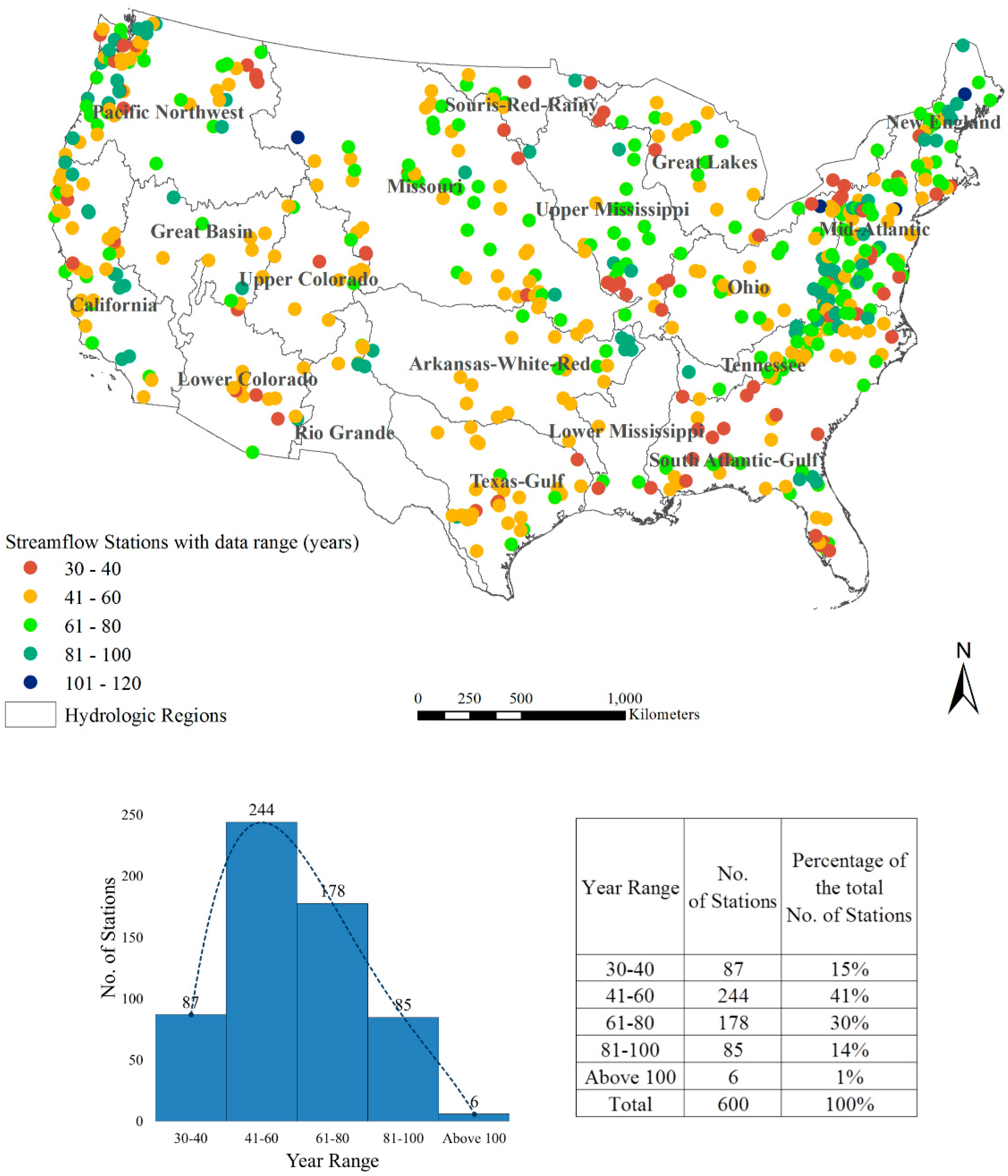
2. Study Area and Data

United States Geological Survey (USGS), (http://water.usgs.gov/) has divided the continental U.S. into 18 hydrologic regions. Published in 2012, the USGS Hydro-climatic Data Network 2009 (HCDN-2009) has listed 704 unimpaired streamflow stations in the continental United States [51]. Out of the 704 stations listed by HCDN 2009, 600 stations were used in this study based on the availability of data (Figure 1). Streamflow data in this network is unaffected by artificial diversions, storage, or other control in or on the natural stream channels or in the watershed.
The raw data were obtained on a monthly time scale, and were averaged to obtain data for the water year, which starts from October of the previous year and extends to September of the current year. Data for seasons were obtained in a similar manner by averaging data of the corresponding months: fall (October–December), winter (January–March), spring (April–June), and summer (July–September). All the results were obtained by analyzing the water year and seasonal mean flows.
Data were obtained over a long range of years in order to cover as many stations having at least 30 years of continuous data with no omissions (missing values) in between. For the analyses, end data entries were fixed at 2012 (since all the stations had data until 2012) and for the beginning year, data were tracked back up to as early as 1903 to obtain the maximum number of stations. As a result, the dataset covered a range of 109 years, while each station had a minimum of 30 years of continuous data. Figure 1 shows the available number of stations in each range of years.

3. Methods

The following sub-sections discuss the test methods used in the study:

3.1. Trend Tests

Several statistical methods that have been used as trend detection tools and many have their advantages based on the application. The Mann-Kendall (MK) trend test [45,46], termed MK1 in this paper, has been used in many previous studies because of its certain advantages, i.e., assumptions regarding the shape of the probability distribution, the ability to account for non-stationarity, and its accuracy. These advantages have made it popular over other traditional methods [2,48]. The MK trend test is a non-parametric test, which is appropriate for analyzing parameters such as streamflow, which are non-stationary in nature [47]. The MK trend test is also useful when analyzing time series with missing values in between data points; this is an effective feature when analyzing longer time series.
The presence of autocorrelation or persistence (clustering behavior) is found to be quite common in hydrologic time series, especially in streamflow and precipitation data, and can suggest the erroneous presence of trends [52]. To encounter the effect of persistence, certain adjustments suggested by previous scholarly works were incorporated into the current study, which dealt with both lag-1 autocorrelation (short-term persistence, or STP) and long-term persistence (LTP, or the Hurst phenomenon). An adjustment known as Trend Free Pre-Whitening was used to remove the presence of STP; the adjusted version of the test is termed MK2 in the subsequent sections of this paper. Details of Pre-Whitening can be found in the works of [33,38,53,54]. To remove the effect of LTP, the Hurst component was applied; this adjusted test is termed MK3 in the subsequent sections. The adjustments that were applied with the underlying hypotheses can be found in the works of [55,56,57].
The MK test determines the direction of trends (increasing or decreasing) based on the sign of the test statistic (positive or negative). The standardized test statistic determines the significance level of rejecting the null hypothesis. TFPW computes the lag-1 autocorrelation (STP) coefficient and tests whether the calculated coefficient lies within the confidence interval found from the sample data. Pre-whitening is applied on data that lied outside the confidence interval (data that were serially dependent). The Hurst component evaluates the presence of LTP and based on the presence of LTP, corrects the bias of the variance. Interested readers may refer to the original texts for detailed explanation of the terms and the governing equations. Confidence intervals and significance levels have been discussed in the Results section.
Thiel-Sen Approach (TSA) [58,59] was employed to calculate the magnitude of the average trend slopes at each temporal scale. Kriging, which also accounts for the effect of autocorrelation, was used to interpolate the values of the slopes in the surrounding areas of a station.

3.2. Shift Test

To determine the presence of shifts or step changes, the non-parametric Pettitt’s test [49] was selected for this study. Comparison between different techniques for change points (or shifts) suggested that Pettitt’s test has much higher accuracy compared to some other traditional methods [26]. Pettitt’s test detects the anomaly (if any) in the median of a time series by testing two samples from the same population. The probability estimate provides the direction of the change based on the significance level considered. The maximum and minimum value of the probability estimate indicates a positive and negative change, respectively.

3.3. Field Significance Test

In addition to the presence of trends and shifts in the time series, the field significance was calculated, which determined whether the regions themselves have an overall significance or not. Walker’s test [60], which takes into consideration the magnitude of the p-value of each of the local trend test to evaluate the global significance level, was used to determine the field significance of each region.
Non-stationary behaviors of hydroclimatic parameters have been described by the authors of [44], and the study suggested the type of significance test to be used in their analysis. In all the methods applied in the current study, the threshold confidence level for significance tests was set at 90%, with p ≤ 0.10. To examine the variation in significance, the trend and shift tests were investigated at 90%, 95%, and 99% confidence levels.

4. Results

Trends and shifts of 600 unimpaired streamflow stations were analyzed to observe their significant increasing and decreasing change patterns in water year and the four seasons (fall, winter, spring, and summer) at multiple time intervals analyzing the water year and seasonal mean flows. Figure 2a–c illustrate the results obtained from MK1, MK2, and MK3, respectively, with stations having significant trends. Figure 2d shows the distribution of average streamflow trend slope values at the different temporal scales after removal of the outliers. Effect of persistence in data is illustrated in Figure 3. Results of shifts, obtained from the Pettitt’s test are illustrated in Figure 4a,b. A p-value of ≤ 0.10 was selected in all the tests to determine the threshold significance. Different level of significance with trends (shifts) was denoted by varying size of the markers representing the stations (small, medium, and large triangles corresponded to 90%, 95%, and 99% levels of confidence, respectively).

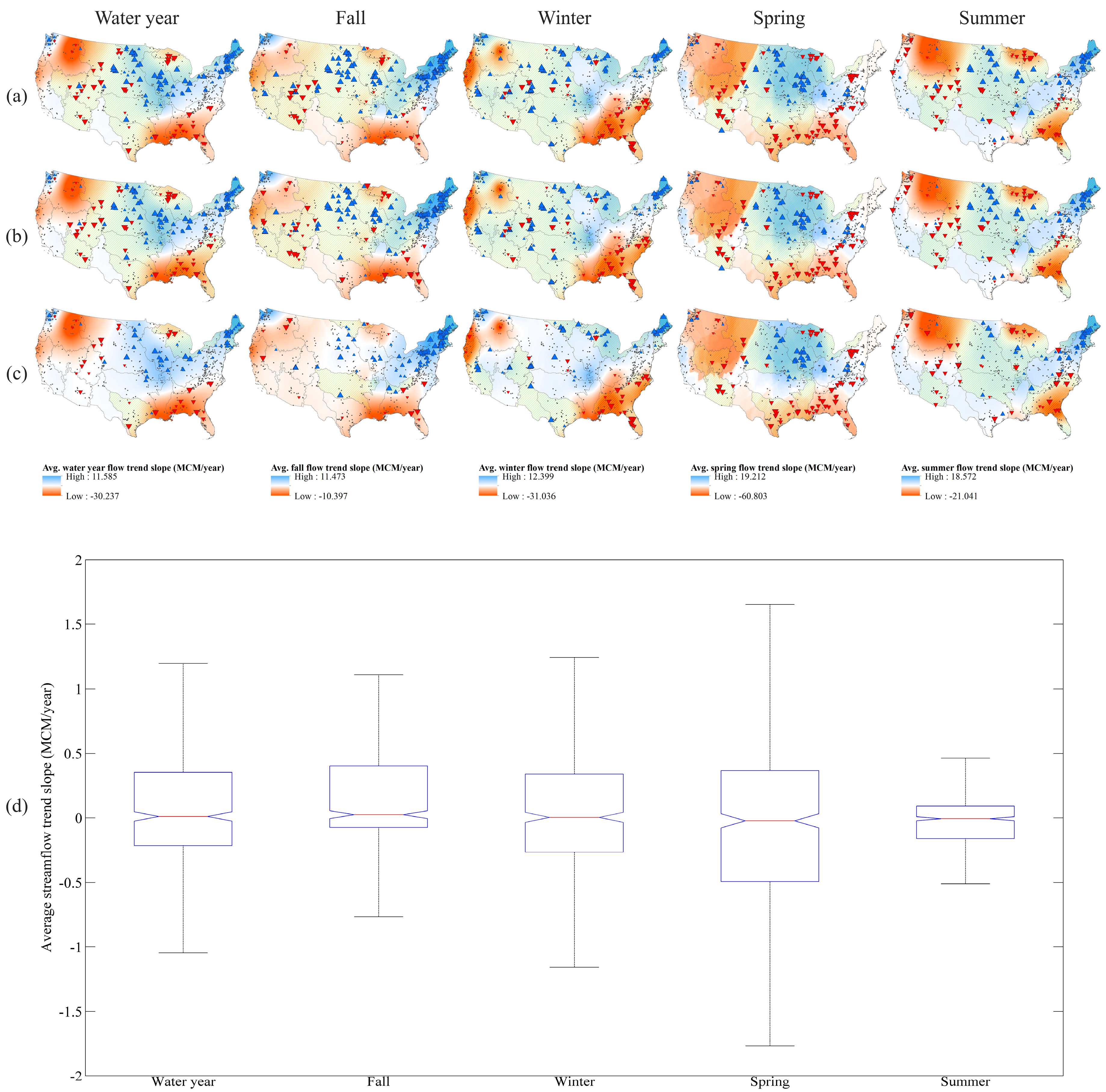
4.1. MK1 Test for Trends

The spatial distribution of trends in water year and the seasonal scales are shown in Figure 2a. The results are shown in Table 1 for each region and their corresponding number of stations, with either increasing or decreasing trends. In water year, 147/600 stations (25%) showed either increasing or decreasing trends, out of which 90 stations (15%) showed increasing trends and 57 stations (10%) showed decreasing trends. New England (1), Mid-Atlantic (2), Ohio (5), Upper Mississippi (7), Souris-Red-Rainy (9), and Missouri (10) showed presence of significant number of stations with increasing trends. The majority of decreasing trends were observed in South Atlantic-Gulf (3), Great Lakes (4), Mississippi (10), Upper Colorado (14), and Pacific Northwest (17). The levels of significance among the stations with trends were observed to vary across the regions without any noticeable pattern. The average water year flow trend slope was observed to vary from −30.237 to 11.585 million cubic meter (MCM)/year (Figure 2). Figure 2d showed the reduction of trend slope value distribution after removal of the outliers. In addition, 10/18 regions (55%) showed presence of field significance. A comparison between Figure 1 and Figure 2a showed that the majority of the stations experiencing increasing trends in water year had data within the range of 61 to 80 years and 81 to 100 years; this suggested that the majority of the increasing trends existed in the interval of 1910 to 2012. The majority of the stations with decreasing trends coincided with stations having data in the range of 30 to 40 years and 41 to 60 years; this suggested that decreasing trends were significant from approximately 1950 to 2012.
In fall, 155/600 stations (26%) were observed to show trends; 121 stations (20%) showed increasing trends and 34 stations (6%) showed decreasing trends (Table 1). New England (1), Mid-Atlantic (2), Ohio (5), Upper Mississippi (7), Souris-Red-Rainy (9), and Missouri (10) showed significant number of stations with increasing trends. Higher number of stations with decreasing trends was observed in South Atlantic-Gulf (3), Great Lakes (4), Upper Colorado (14), and Lower Colorado (15), as seen in Figure 2a. The level of significance among the stations with trends varied across the study area. The average fall flow trend slope was observed to vary between −10.397 to 11.473 MCM/year (Figure 2). Removal of outliers narrowed down the distribution significantly (Figure 2d). Field significance was observed in 12/18 regions (67%). The analyses of different time intervals with increasing trends during fall, found by a comparison between Figure 1 and Figure 2a, showed that the majority of the stations with trend coincided with stations having data in the range of 61 to 80 years and 81 to 100 years. This suggested that increasing trends were significant in the interval of 1910 to 2012. The majority of the stations with decreasing trends coincided with stations having a data range from 30 to 40 years and 41 to 60 years; this suggested presence of decreasing trends from approximately 1950 to 2012.
For winter, 140/600 stations (23%) were observed to show either increasing or decreasing trends, out of which 93 stations (16%) showed increasing trends and 47 stations (8%) showed decreasing trends (Table 1). New England (1), Great Lakes (4), Souris-Red-Rainy (9), and Missouri (10) showed presence of significant number of stations with increasing trends. The majority of decreasing trends were observed in South Atlantic-Gulf (3). Other regions of the continental U.S. showed presence of mixed patterns, with both increasing and decreasing trends (Figure 2a). Stations with trends at different significant levels varied across the regions. The average winter flow trend slope varied from −31.036 to 12.399 MCM/year (Figure 2). Figure 2d showed the effect of outlier removal from the distribution. 13/18 regions (72%) showed presence of field significance. A comparison between Figure 1 and Figure 2a showed that the majority of the stations with increasing trends during winter coincided with stations with a data range from 41 to 60 and 61 to 80; this suggested that increasing trends were significant in the interval of 1930 to 2012. The majority of the stations with decreasing trends coincided with stations having a data range from 30 to 40 years, 41 to 60 years, and 61 to 80 years; this suggested presence of significant decreasing trend from approximately 1930 to 2012.
During spring, 150/600 stations (22%) indicated presence of trends, out of which 56 stations (9%) showed increasing trends and 94 stations (16%) showed decreasing trends (Table 1). The majority of increasing trends were observed in Ohio (5), Upper Mississippi (7) and Missouri (10). Mid-Atlantic (2), South Atlantic-Gulf (3), Great Lakes (4), Texas-Gulf (12), Upper Colorado (14), and Lower Colorado (15) showed strong presence of stations with decreasing trends (Figure 2a). The significance levels of the stations with trends were observed to vary across different regions. The average spring flow trend slope varied from −60.803 to 19.212 MCM/year. Spring showed the largest distribution in terms of the variation in trend slope values. The large distribution was observed to prevail even after removal of the outliers, though the distribution narrowed down significantly (Figure 2d). Presence of field significance was observed in 10/18 regions (55%). The majority of stations with increasing trends in spring coincided with stations having a data range from 61 to 80, which suggested significant increasing trend in the interval of 1930 to 2012 (Figure 1 and Figure 2a). The majority of stations with decreasing trends corresponded with stations with data ranges from 30 to 40 years and 41 to 60 years; this suggested presence of significant decreasing trends from approximately 1950 to 2012.
In summer, 131/600 stations (22%) were observed to show trends, out of which 65 stations (11%) exhibited increasing trends and 66 stations (11%) showed decreasing trends (Table 1). New England (1), Mid Atlantic (2), Upper Mississippi (7), Souris-Red-Rainy (9), and Missouri (10) showed significant presence of stations with increasing trends; the majority of decreasing trends were observed in South Atlantic-Gulf (3), Great Lakes (4), Upper Colorado (14), Great Basin (16), and Pacific Northwest (17) (Figure 2a). Similar to other seasons, the level of significance among the stations varied across different regions without any noticeable pattern. The average summer flow trend slope was observed to vary between −21.041 to 18.572 MCM/year. Summer had the narrowest distribution of trend slope values amongst all the seasons. The narrow distribution was also observed after removal of the outliers (Figure 2d). Eleven out of eighteen regions (61%) were observed to have field significance. In summer, the majority of stations with increasing trends corresponded to stations having data ranges from 61 to 80 years and 81 to 100 years; this suggested presence of increasing trends during the interval of 1910 to 2012. The majority of stations with decreasing trends coincided with stations with data ranges from 30 to 40 years, 41 to 60 years, and 81 to 100 years, suggesting a significant presence of decreasing trends from approximately 1910 to 2012 (Figure 1 and Figure 2a).

4.2. MK2 Test for Trends

The spatial distribution of trends in water year and the four seasons under MK2 are shown in Figure 2b, and the results are listed in Table 1. In water year, 14% (10%) of the stations showed presence of increasing (decreasing) trends (Table 1). The majority of these stations with increasing trends were located in New England (1), Mid-Atlantic (2), Ohio (5), Upper Mississippi (7), Souris-Red-Rainy (9), and Missouri (10). South Atlantic-Gulf (3), Great Lakes (4), Missouri (10), and Upper Colorado (14) showed strong presence of decreasing trends (Figure 2b). Fifty-six percent of the regions showed presence of field significance, which was significantly higher than what was observed under MK1 in water year. The majority of increasing (decreasing) trends was significant in the interval of 1910 to 2012 (1950 to 2012).
In fall, 20% (6%) of the stations showed increasing (decreasing) trends (Table 1). New England (1), Mid-Atlantic (2), Ohio (5), Upper Mississippi (7), Souris-Red-Rainy (9), and Missouri (10) showed strong presence of increasing trends, while South Atlantic-Gulf (3), Great Lakes (4), Upper Colorado (14), and Lower Colorado (15) showed strong presence of deceasing trends (Figure 2b). Sixty-seven percent of the regions showed presence of field significance. Increasing (decreasing) trends were significant during the interval of 1910 to 2012 (1950 to 2012) (Figure 1 and Figure 2b).
In winter, 14% (8%) of the stations showed presence of increasing (decreasing) trends (Table 1). Majority of the stations showing increasing trends were located in New England (1), Great Lakes (4), Souris-Red-Rainy (9), Missouri (10), Pacific Northwest (17), and California (18); strong decreasing trends were observed in South Atlantic-Gulf (3) (Figure 2b). Seventy-two percent of the regions showed presence of field significance. Both increasing and decreasing trends were found to be significant during the interval of 1930 to 2012 (Figure 1 and Figure 2b).
In spring, 10% (16%) of the stations showed presence of increasing (decreasing) (Table 1). Strong increasing trends were observed in Ohio (5), Upper Mississippi (7) and Souris-Red-Rainy (9). Missouri (10). Mid-Atlantic (2), South Atlantic-Gulf (3), Great Lakes (4), Texas-Gulf (12), Great Basin (16), and Lower Colorado (15) showed strong presence of decreasing trends (Figure 2b). Fifty percent of the regions showed presence of field significance. Strong increasing (decreasing) trends were observed in the interval of 1930 to 2012 (1950 to 2012) (Figure 1 and Figure 2b).
In summer, 11% (11%) stations showed presence of increasing (decreasing) trends (Table 1). Strong presence of increasing trends was observed in New England (1), Mid-Atlantic (2), Upper Mississippi (7), Souris-Red-Rainy (9), and Missouri (10). South Atlantic-Gulf (3), Great Lakes (4), Upper Colorado (14), and Pacific Northwest (17) showed strong presence of decreasing trends (Figure 2b). Field significance was observed in 56% of the regions. A strong presence of both significant increasing and decreasing trends were observed in the interval of 1910 to 2012 (Figure 1 and Figure 2b).

4.3. MK3 Test for Trends

The spatial distribution of trends at water year and the seasonal scales under MK3 are shown in Figure 2c. Table 1 lists each region with their corresponding number of stations with trends. In water year, 9% (6%) stations showed presence of increasing (decreasing) trends (Table 1). The majority of the stations with increasing trends were observed in New England (1), Ohio (5), and Upper Mississippi (7). South Atlantic-Gulf (3), Missouri (10), and Upper Colorado (14) showed higher number of stations with significant decreasing trends. Field significance was observed in 17% of the regions. The majority of the stations with increasing (decreasing) trends occurred during the interval of 1910 to 2012 (1950 to 2012) (Figure 1 and Figure 2c).
In fall, 14% (3%) stations showed presence of increasing (decreasing) trends (Table 1). New England (1), Mid-Atlantic (2), Ohio (5), and Missouri (10) showed strong presence of increasing trends, while the majority of the stations with decreasing trends were observed in South Atlantic-Gulf (Figure 2c). Twenty-two percent of the regions showed presence of field significance. The majority of the increasing (decreasing) trends occurred in the interval of 1910 to 2012 (1950 to 2012) (Figure 1 and Figure 2c).
In winter, 9% (6%) stations showed presence of increasing (decreasing) trends (Table 1). Increasing trends were found strong in New England (1), Great Lakes (4), Pacific Northwest (17), and California (18). South Atlantic-Gulf (3) showed strong presence of decreasing trends (Figure 2c). Forty-four percent of the regions showed presence of field significance. Presence of the most significant trends, both increasing and decreasing, was observed during 1930 to 2012 (Figure 1 and Figure 2c).
In spring, 7% (14%) stations showing presence of increasing (decreasing) trends (Table 1). Ohio (5), Upper Mississippi (7) and Missouri (10) showed strong presence of increasing trends. Decreasing trends were strong in Mid-Atlantic (2), South Atlantic-Gulf (3), Great Lakes (4), Texas-Gulf (12), Upper Colorado (14), Lower Colorado (15), and Pacific Northwest (17) (Figure 2c). Thirty-nine percent of the regions showed presence of field significance. Most of the stations with increasing (decreasing) trends were found to be significant in the interval of 1930 to 2012 (1950 to 2012) (Figure 1 and Figure 2c).
In summer, 8% (9%) stations showed presence of increasing (decreasing) trends (Table 1). Strong Increasing trends were observed in New England (1), Mid-Atlantic (2), and Ohio (5). South Atlantic-Gulf (3), Great Lakes (4), Upper Colorado (14), and Pacific Northwest (17) showed presence of strong decreasing trends (Figure 2c). Forty-four percent of the regions showed presence of field significance. The majority of the stations with significant trends, both increasing and decreasing, were observed during the interval of 1910 to 2012 (Figure 1 and Figure 2c).

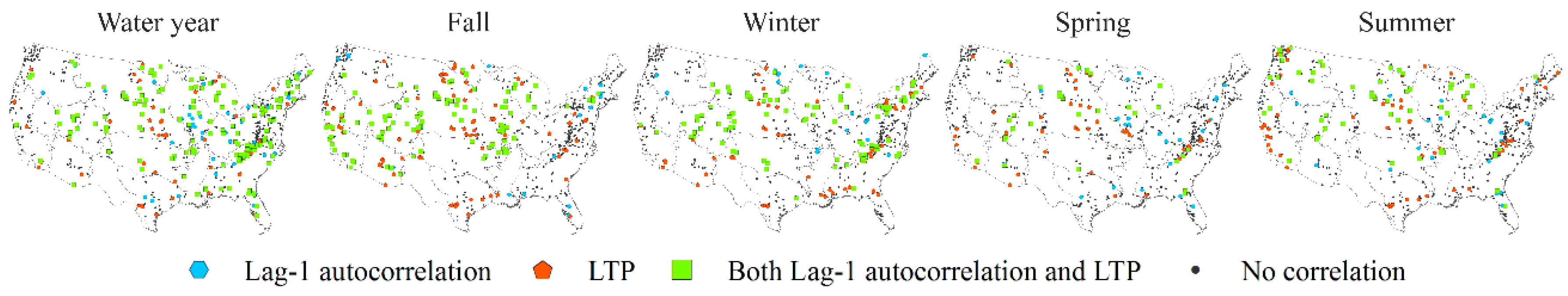
4.4. Persistence in Trends

To remove the presence of lag1-autocorrelation (STP) and LTP, modified MK tests were applied on the time-series data. Figure 3 shows the distribution of stations across the continental U.S. with the presence of STP, LTP, or both. Table 1 compares the results found under each MK test, and shows the effect of removal of persistence from the data. Appropriate ranges for autocorrelation coefficient and Hurst component, which were found statistically correlated at p ≤ 0.10, were calculated based on the variable length of data.
In water year, 207/600 stations (35%) showed presence of STP and 210/600 stations (35%) showed presence of LTP. Most of the eastern regions—New England (1), Mid-Atlantic (2), South Atlantic-Gulf (3), Great Lakes (4), Ohio (5), and Tennessee (6)—showed higher number of stations with the presence of STP, LTP, or both (Figure 3). Presence of persistence was observed to decrease from east to west across the continental United States. Moreover, the extreme western states i.e., Pacific Northwest (17) and California (18) hardly showed any presence of persistence in data. The majority of the stations with LTP were observed to coincide with the station having a data length of 41 to 60 years and 61 to 80 years (Figure 1 and Figure 3). Stations with STP were also found in similar ranges (availability) of data lengths; but, unlike LTP, presence of STP was also observed in shorter data lengths, i.e., 30 to 40 years range.
During fall, 138/600 stations (23%) showed presence of STP and 208/600 stations (35%) showed presence of LTP. Upper Mississippi (7), Missouri (10), Upper Colorado (14), Great Basin (16), and California (18) showed higher number of stations with persistence compared to other regions (Figure 3). Eastern regions, especially the southeastern regions, showed only a few stations with persistence. Presence of LTP was observed in stations having data length of 41 to 60 years, 61 to 80 years, and 81 to 100 years. Presence of STP was observed in higher data ranges similar to LTP, as well as in lower ranges of 30 to 40 years.
In winter, 130/600 stations (22%) showed presence of STP and 165/600 stations (28%) showed presence of LTP. A higher number of stations with persistence was observed in Mid-Atlantic (2), Great Lakes (4), Tennessee (6), Missouri (10), Upper Colorado (14), and Great Basin (16) (Figure 3). Extreme western regions, i.e., Pacific Northwest (17) and California (18) had only a few stations with persistence. The majority of the stations with LTP were observed to have a data length of 41 to 60 years and 61 to 80 years. Stations with STP were observed in stations having data length of as low as 30 to 40 years to as high as 81 to 100 years.
In spring, 64/600 stations (11%) showed presence of STP and 78/600 stations (13%) showed presence of LTP. Compared to other regions, South Atlantic-Gulf (3), Upper Mississippi (7), and Missouri (10) showed higher number of stations with persistence (Figure 3). Compared to fall and winter, number of stations with persistence in spring was much lower. The majority of stations with LTP were observed in stations having data range of 30 to 40 year, 41 to 60 years, and 61 to 80 years. The presence of STP was observed in stations having similar data range.
In summer, 84/600 stations (14%) showed presence of STP and 115/600 (19%) stations showed presence of LTP. Compared to other regions, South Atlantic-Gulf (3), Great Lakes (4), Missouri (10), Pacific Northwest (17), and California (18) showed presence of higher persistence (Figure 3). Both LTP and STP were observed in stations having data length of 41 to 60 year and 61 to 80 years.

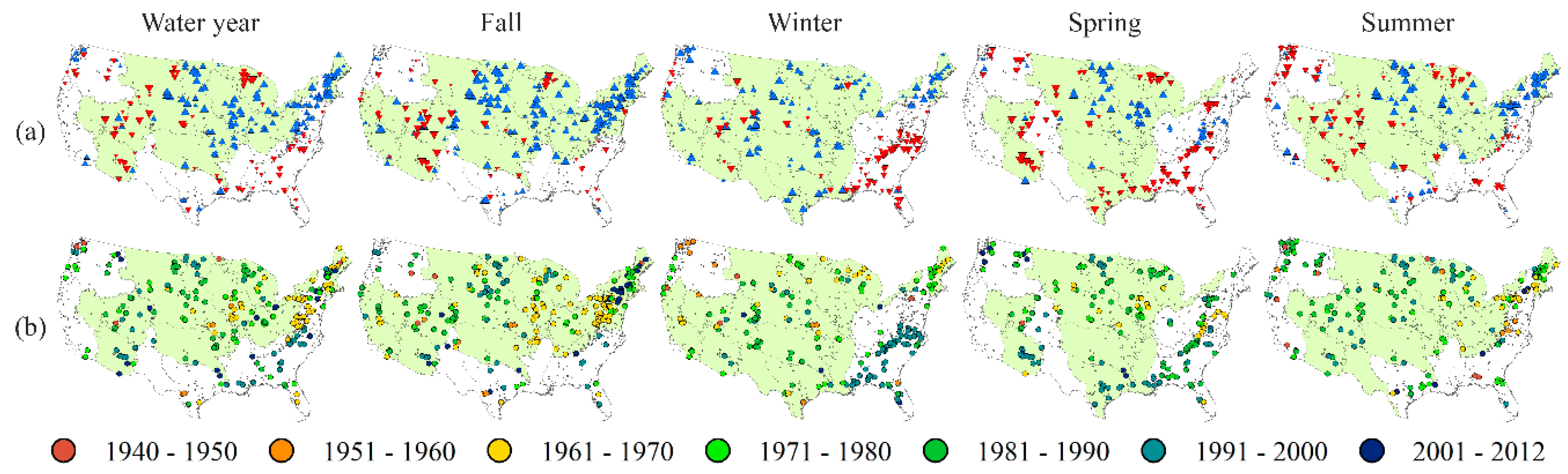
4.5. Pettitt’s Test for Shifts

The spatial distribution of shifts in water year and the seasonal scales are shown in Figure 4, and the effect of shift in each region is shown in Table 2. In water year, the pattern showed a high concentration of stations with increasing shifts in the northeast and upper-central regions. The majority of stations with decreasing shifts were concentrated in the southeast and mid-western regions.
In water year, 226/600 stations (38%) showed presence of shifts, out of which 137 stations (23%) showed presence of increasing shifts and 89 stations (15%) showed presence of decreasing shifts (Table 2). The majority of increasing shifts were observed in New England (1), Mid-Atlantic (2), Ohio (5), Upper Mississippi (7), Souris-Red-Rainy (9), and Missouri (10). South Atlantic-Gulf (3), Great Lakes (4), Upper Colorado (14), Lower Colorado (15), Great Basin (16), and Pacific Northwest (17) showed strong presence of stations with decreasing shifts (Figure 4a). Stations with different levels of significance varied across the regions without any noticeable pattern. Ten out of eighteen regions (56%) showed presence of field significance.
The spatio-temporal map (Figure 4b) of shift in water year showed that major changes occurred from 1961 to 2000. In this range, 200/600 stations (33.33%) showed presence of either increasing or decreasing shifts. Before 1960, only 9/600 stations (1.5%) showed presence of significant changes. After 2000, the number of stations with shift decreased compared to the previous few decades. Figure 4b showed that the changes that occurred had some spatial patterns as well. Shifts observed from 1961 to 1970 were highly concentrated in New England (1), Mid-Atlantic (2), and Upper Mississippi (7). Changes that occurred from 1971 to 2012 were found to be quite spatially distributed, with a comparatively higher tendency of change in the northern and central regions. Table 3 shows the results of shifts that were observed during different time intervals in water year.
In fall, 169/600 stations (28%) showed presence of shifts, out of which 70 stations (12%) showed presence of increasing shifts and 99 stations (17%) showed presence of decreasing shifts (Table 2). New England (1), Mid-Atlantic (2), Ohio (5), Upper Mississippi (7), Souris-Red-Rainy (9), and Missouri (10) showed presence of significant number of stations with increasing shifts. The majority of decreasing shifts were observed in South Atlantic-Gulf (3), Great Lakes (4), Upper Colorado (14), Lower Colorado (15), and Great Basin (4) (Figure 4a). Level of significance of shifts was observed to vary across the regions. Thirteen out of eighteen regions (72%) showed presence of field significance.
The majority of the shifts that occurred during fall were found to be from 1961 to 2012 (Figure 4b and Table 3). During this interval, 222/600 stations (35%) showed presence of either increasing or decreasing shifts. Changes occurring from 1961 to 1970 were observed to be highly concentrated in Mid-Atlantic (2), Great Lakes (4), Ohio (5), and Upper Mississippi (7). Changes from 2000 to 2012 were found to be denser in New England (1) and Mid-Atlantic (2); meanwhile, changes from 1971 to 2000 were quite spatially distributed across the continental United States. Not many shifts were observed before 1961.
In winter, 209/600 stations (35%) showed shifts, out of which 125 stations (21%) showed presence of increasing shifts and 84 stations (14%) showed presence of decreasing shifts (Table 2). New England (1), Great Lakes (4), Souris-Red-Rainy (9), and Missouri (10) showed strong presence of stations with increasing shifts, while decreasing shifts were strong in South Atlantic-Gulf (3), Great Basin (16), and Pacific Northwest (17) (Figure 4a). Different levels of significance did not show any noticeable pattern across the regions. Field significance was observed in 13/18 regions (72%).
Winter showed higher number of stations with shifts from 1951 to 2000 (Figure 4b and Table 3). Before 1951, there was rarely any presence of significant change across the study area. From 1971 to 2000, the changes occurred were observed to be significantly high. A total of 161/600 stations (27%) showed presence of shifts during this interval. The most prominent spatial pattern observed was in South Atlantic-Gulf (3), occurring from 1991 to 2000. Changes occurring from 1951 to 1960 and from 1961 to 1970 were observed to be comparatively higher in northwestern and northeastern regions, respectively. Shifts in other time intervals were quite spatially distributed across the study area.
In spring, 186/600 stations (31%) showed presence of shifts; with 67 stations (11%) showing presence of increasing shifts and 119 stations (20%) showing presence of decreasing shifts (Table 2). Ohio (5), Upper Mississippi (7), Souris-Red-Rainy (9), and Missouri (10) had strong presence of stations with increasing shifts, while decreasing shifts were strong in Mid-Atlantic (2), South Atlantic-Gulf (3), Great Lakes (4), Texas-Gulf (12), Upper Colorado (14), Lower Colorado (15), and Pacific Northwest (17) (Figure 4a). Different levels of significance among the stations were observed to be not showing any spatial pattern. Nine of out of eighteen regions (50%) showed presence of field significance.
The majority of the changes observed in spring were found to be during the time interval from 1961 to 2000 (Figure 4b). In this interval, 172/600 stations (29%) showed presence of significant increasing or decreasing shifts (Table 3). The maximum number of stations with shifts was observed from 1981 to 1990 (66/600 stations). In addition, the stations having shifts during this interval showed a high concentration in South Atlantic-Gulf (3), Great Lakes (4), and Missouri (10). During different time intervals, the presence of small clustered behavior was observed in Mid-Atlantic (2), Great Lakes (4), Souris-Red-Rainy (9), Lower Colorado (15), and Pacific Northwest (17) (Figure 4b). Before 1961, there was rarely any presence of significant shift in spring.
In summer, 198/600 stations (33%) showed presence of shifts, with 96 stations (16%) showing increasing shifts and 102 stations (17%) showing decreasing shifts (Table 2). The majority of increasing shifts were observed in New England (1), Mid-Atlantic (2), Souris-Red-Rainy (9), and Missouri (10), while a strong presence of decreasing shifts were observed in South Atlantic-Gulf (3), Great Lakes (4), Upper Colorado (14), Great Basin (16), and Pacific Northwest (17) (Figure 4a). Stations with different levels of significance did not show any noticeable pattern. Twelve out of eighteen regions (67%) showed presence of field significance.
Summer showed higher number of stations having significant shifts from 1961 to 2000 (Figure 4b). Out of 600 stations, 175 stations (29%) showed presence of changes during this interval; maximum number of stations with shifts were observed from 1981 to 1990 (66/600 stations) (Table 3). Changes occurred from 1961 to 1970 were observed to be concentrated in New England (1), Mid-Atlantic (2), Great Lakes (4), and Ohio (5). Changes occurring from 1971 to 2000 were observed to be quite spatially distributed across the study period, with a higher tendency towards central and western regions. Compared to other seasons, summer showed higher presence of shifts from 1921 to 1950 (11/600 stations).

5. Discussion

Detection of change patterns (trends and shifts) among the unimpaired streamflow stations in the continental U.S. at different temporal scales was the primary objective of the current study. An approach of using a minimum number of years (threshold) of data was employed to cover as many streamflow stations as possible. This allowed the study to take a closer look at the regional changes that have occurred historically. Statistical methods were applied to the original data (time-series), which was obtained over a long period of time, in order to study the change patterns in water year and the four seasons at different time intervals (data were obtained on a monthly basis and were analyzed using water year and seasonal mean flows). Persistence in data, which can lead to an erroneous detection of trends, was also considered and accounted for while analyzing the data.
The results indicated that stations in the northeast and upper-mid regions experienced an increasing trend (shift) during the study period (across all temporal scales), while the southeast, central mid-west and northwest regions experienced a decreasing trend (shift) (Figure 2 and Figure 4). The spatial distribution of stations with significant change, as well as the value of average flow trend slopes, varied across the seasons (Figure 2). Even though the different level of significance did not show any noticeable spatial pattern, significance of the same stations was observed to vary across different temporal scales, which suggests the importance of trend (shift) analyses at multiple temporal scales. Use of different time intervals showed that majority of increasing trends occurred from 1910 to 2012, and decreasing trends occurred from 1950 to 2012 (Figure 1 and Figure 2). The change points of shifts showed that majority of the changes occurred from 1961 to 2000 (Figure 4). The spatial distribution of stations with significant trend in water year under MK1 revealed that stations in the northeast (New England and Mid-Atlantic) to the upper-central regions (Upper Mississippi, Souris-Red-Rainy and Missouri) likely went through increasing change over the study period (Figure 2a). Similar results were found by the authors of [2], who observed that the northeast U.S. annual low flows were undergoing an increase. These results were also confirmed by the authors of [61]. Additionally, an increase in streamflow in the eastern U.S. was found by the authors of [62]; they concluded that the increase in streamflow was a result of increased precipitation in the surrounding regions. Significant decreasing trends were observed in the southeast (South Atlantic-Gulf), the mid-west (Upper Colorado and Lower Colorado), and the northwest (Pacific Northwest) regions. Some regions (e.g., Missouri) were observed to have both increasing and decreasing trends. These results showed how change patterns can vary within and across the regions at different time intervals across different temporal scales. Studies have also suggested understanding of regional change patterns for public regulations on regional scale for better policy making [36,37]. The underlying trend patterns observed in this study and supported by previous works can potentially help understand the historical change patterns of hydrologic parameters in the regions studied.
Presence of field significance was observed in regions with higher number of stations having significant trends. Overall streamflow of the continental U.S. was found to increase with comparatively less intensity by the authors of [1]; this was observed in the current study as well, since in water year, the overall percentage of stations with increasing trends (15% of the total stations) were found to be higher than the overall percentage of stations with decreasing trends (9% of the total stations) (Table 1). Moreover, the current results were supported by the authors of [17], who concluded that the greater proportions of the conterminous U.S. streamflow stations were experiencing an increasing trend. Similar results were obtained in this study in the water year mean via average water year flow trend slope values (Figure 2d). The three different levels of confidence (90%, 95%, and 99%) used in this study also showed how higher confidence levels of individual stations influenced the field significance of a particular region. Even though the different significance (confidence) levels did not show any spatial pattern, they definitely influenced the field significance of the region (regions with a higher number of stations at 99% confidence level were observed to have a higher tendency to field significance). The results can be helpful in identifying regions with stations having higher significant trends.
Results from the analyses of different time intervals of the trends indicated that increasing trends in water year under MK1 were strong during the interval of 1910 to 2012, while decreasing trends were strong from 1950 to 2012 (Figure 1 and Figure 2a). This suggested that the duration of increasing trends has been much higher compared to the duration of decreasing trends along the study period in the water year mean. The duration and frequency (fluctuation patterns) of these trends can be correlated with decadal and multi-decadal oceanic-atmospheric oscillations, i.e., El Niño Southern Oscillation, Pacific Decadal Oscillation and North Atlantic Oscillation. Some of the previous studies [2,11,35,63] have investigated the coupled behavior among these oscillations and hydrologic variables at different temporal scales across different regions. Change patterns at different time intervals on multiple temporal scales observed in this study can certainly provide insights in correlating results of previous studies as the current study dealt with the duration and the most significant intervals of trends.
Analysis of the seasons, which is highly important for agriculture and energy demand [16,19,20], revealed changing behaviors of the streamflows along the seasons. From the analyses under MK1 (Figure 2a), it was observed that fall and summer had similarities with the trend patterns of water year; in contrast, winter and spring showed quite a different distribution. Fall was found to be the wettest season and spring was found to be the driest based on the observation of the trends (shifts). Average flow trend slopes revealed that the highest variance was observed during spring while summer had the lowest variance (Figure 2). Removal of outliers showed that fall and winter had higher tendency towards increasing flow while spring and summer had higher tendency towards decreasing flow (Figure 2d). The results of the current study were found consistent with previous works [25]. The underlying reasons affecting the seasonal variations (observed in the variance of distribution) can be attributed to climate variability and change.
The effect of variable length of data (different time intervals across the study area) revealed that the duration of trends varied across the seasons (Figure 1 and Figure 2). Fall experienced the majority of its increasing trends from 1910 to 2012 and the majority of its decreasing trends from 1950 to 2012. During winter, both increasing and decreasing trends were observed to be strong in the interval of 1930 to 2012. In spring, strong increasing trends were observed from 1930 to 2012, while the majority of the decreasing trends were observed from 1950 to 2012. Summer experienced the majority of its increasing and decreasing trends from 1910 to 2012. As the effects of seasonal change were observed to vary across the regions, different time intervals showed how they have changed over time. Moreover, the results indicated how long the trends in seasons were and how they influenced regions spatially across the study area. These findings can be helpful in regional understanding of trend patterns especially to meet water demand, as it varies significantly across the seasons.
The results revealed that removal of only lag-1 autocorrelation (STP) might not be enough to understand the trend patterns in a time series (Figure 3). Especially while dealing with long time periods, removal of LTP becomes equally important since it can overestimate the presence of significant trends if not removed from the data [28]. The presence of LTP can significantly overestimate the presence of a trend [64], which was also observed in the results of the current study (Figure 2). Distribution of persistence in data, both lag-1 autocorrelation (STP) and LTP revealed that water year data had the maximum persistence among the temporal scales used, while fall and winter had comparatively higher persistence than spring and summer (Figure 3). The distribution also suggested that persistence is quite spatially dispersed across the study area. The comparison of results between with and without persistence also justified the importance of choosing the modified test methods employed in the study. Across all the temporal scales, the majority of the stations with persistence were observed to show presence of both STP and LTP. The available length of data associated with the stations showing STP and LTP varied over a wide range. The results did not suggest any particular pattern. The majority of the stations with persistence were observed to have data length of 41 to 60 years and 61 to 80 years. Both STP and LTP were observed in stations having data length of as low as 30 to 40 years to as high as 81 to 100 years. Compared to LTP, the presence of STP in stations with data range of 30 to 40 years were higher. The concurrent data range of STP and LTP observed in the study can be helpful in understanding their relationship.
The temporal variation of trends under MK2 and MK3 were found to be consistent with the results of MK1, and showed that the majority of the increasing trends occurred from 1910 to 2012, while decreasing trends were found to be strong during the interval of 1950 to 2012 (Figure 1 and Figure 2b,c). The change patterns in seasons under MK2 and MK3 with varying time intervals also followed patterns observed in MK1. Since MK2 and MK3 took into account the effect of STP and LTP, respectively, the temporal variation of trends across the stations were meant to be similar to MK1. The results showed that, indeed, MK2 and MK3 revealed the same timely variation. Though the generic pattern of trends observed under the three MK tests was found to be similar (Figure 2a–c), the number of stations with significant trend in each region varied significantly (Table 1). These changes in numbers explained the effect of persistence in data, and were found to be consistent with previous studies [25]. The presentation of results, which also showed how they varied across regions, found that MK2 and MK3 explained the effect of STP and LTP separately.
The spatial distribution of stations with significant change found in the analyses of shifts was in agreement with the spatial distribution found in the trend analyses (Figure 4a), though the length of the trend patterns were found to be of longer durations. Moreover, in some cases, several regions were observed to show the presence of trends and shifts during the same time interval. Even though trend and shift are apparently two different types of change patterns, there might be implications regarding how they affect each other. A trend of significant length might cause a shift in the hydrologic properties of the regime, while a shift in the regime might result in the development of a new trend. The lag-response behavior of these two types of change patterns, which can be achieved by narrowing down the length of the time interval, might be a potential field of study for the future. The temporal variation of shifts across the study period showed that the majority of the shifts, both increasing and decreasing, occurred during the interval of 1961 to 2000 (Figure 4b). Regions concentrated with stations showing the presence of shifts during a particular time interval suggested that the changes occurred were quite localized in nature, and occurred during a particular time period (interval).
Similar to water year, the effect of time intervals over the shift patterns were observed for the seasons. The results indicated that the most influential time intervals for fall, winter, spring, and summer, were from 1961 to 2012, from 1951 to 2000, from 1961 to 2000, and from 1961 to 2000, respectively. Similar seasonal variations (both on local and continental scales) were also reported by the authors of [20,25,65]. Moreover, the current analyses identified the regions with a higher concentration of stations with shifts (both increasing and decreasing) during specific time intervals. These results could be helpful in understanding the change in behavior in each region, and could be used to analyze localized historical extreme events, as this study presented analyses both including and excluding the outlier (extreme) values of flow. Additionally, this study is intended to lay the groundwork for further analyses at multiple temporal and spatial scales, which could be helpful in understanding streamflow patterns under changing climate. Understanding the physical mechanisms causing the trends and shifts at different time periods can be a potential area of research to explain the implications of hydrologic systems as a whole. A further extension of the study can look into the correlation between streamflow patterns and the change in climate indices during the significant time intervals observed in this study.

6. Conclusions

Data from 600 unimpaired streamflow stations across the continental U.S. were analyzed in the current study to determine the long-term change patterns over a wide range of years. The minimum threshold of continuous data dictated the total number of stations to be analyzed. In this study, each station had a minimum continuous data of 30 years. The study period extended over 109 years (stations had continuous data ranging from 30 to 109 years), with the ending year fixed at 2012 and the beginning year tracked back to as early as 1903.
The study analyzed data over a wide range of years covering stations across the entire continental U.S. to provide a better understanding of the regional change patterns at different temporal scales (water year and the four seasons) along different time intervals. The data obtained were of a monthly nature and were converted to water year and seasonal mean flows. In water year, results showed the presence of increasing trends and shifts in the northeast and the upper-mid regions of the continental United States, while decreasing trends and shifts were strong in the southeast and the mid-western regions. The seasonal analyses showed that the change patterns vary quite significantly across the seasons. Fall was found to be the wettest season, while spring was found to be the driest. For both water year and the seasons, the change patterns were found to be stronger in certain intervals along the study period.
The most important contributions of the study are listed below:
  • Use of minimum threshold year as a criterion for selecting the number of stations: This allowed obtaining data from a large number of stations, which subsequently permitted a thorough observation of regional change patterns both at spatial and temporal scales.
  • Use of multiple temporal scales to analyze the change patterns: Historical time series data were analyzed in water year and the seasonal scales across the study period to observe the variation (in mean flow) of change at different temporal scales.
  • Determination of magnitude and significance of trends: In addition to detecting the presence of trends in historical data, the magnitude of trends (via average flow trend slopes) was evaluated. Stations with significance were classified based on different confidence level with a threshold of 90%.
  • A comprehensive analysis of shifts: Change points of shifts could be traced with greater precision, which lead to a thorough analysis of shifts. The variable length of data allowed observation of the shift patterns at different time intervals across the study period.
  • Integration of multiple modified test methods: Appropriate modifications were applied to account for persistence in data, which subsequently reduced the probability of over-estimation of trends.
The results of this study provided insights regarding the change patterns of streamflow across the continental United States, and can be helpful to water managers to understand the change patterns in regional scales over the study period at different temporal variations. The scope of this work can be extended to analyze the underlying reasons behind change patterns, which could provide important information regarding the physical mechanisms behind these trends and shifts and could also shed light on the correlation of spatial and temporal distributions of these changes.

Acknowledgments

The authors would like to thank the two reviewers for their valuable comments. The authors would also like to thank United States Geological Survey (USGS) for providing the data (HCDN-2009) used in this paper. The authors are grateful to Julie Longo for providing assistance with the proofreading of the manuscript.

Author Contributions

The research idea is designed by second (A.K.) and third author (S.A.) and the results are prepared by first author (K.T.). All the authors analyzed the results and wrote the paper together.

Conflicts of Interest

The authors declare no conflict of interest.

Abbreviations

The following abbreviations are used in this manuscript:
WMOWorld Meteorological Organization
USGSsUnited States Geological Survey
HCDNHydro-climatic Data Network
MKMann-Kendall
STPShort-term persistence
LTPLong-term persistence

References

  1. Rice, J.S.; Emanuel, R.E.; Vose, J.M.; Nelson, S.A.C. Continental U.S. streamflow trends from 1940 to 2009 and their relationships with watershed spatial characteristics. Water Resour. Res. 2015, 1944–7973. [Google Scholar] [CrossRef]
  2. Lins, H.; Slack, J. Streamflow trends in the United States. Geophys. Res. Lett. 1999, 26, 227–230. [Google Scholar] [CrossRef]
  3. Carrier, C.; Kalra, A.; Ahmad, S. Long-range precipitation forecast using paleoclimate reconstructions in the western United States. J. Mt. Sci. 2016, 13, 614–632. [Google Scholar] [CrossRef]
  4. Cayan, D.R.; Kammerdiener, S.A.; Dettinger, M.D.; Caprio, J.M.; Peterson, D.H. Changes in the Onset of Spring in the Western United States. Bull. Am. Meteorol. Soc. 2001, 82, 399–415. [Google Scholar] [CrossRef]
  5. Milly, P.C.D.; Wetherald, R.T.; Dunne, K.A.; Delworth, T.L. Increasing risk of great floods in a changing climate. Nature 2002, 415, 514–517. [Google Scholar] [CrossRef] [PubMed]
  6. McCabe, G.J.; Wolock, D.M. A step increase in streamflow in the conterminous United States. Geophys. Res. Lett. 2002, 29, 2185. [Google Scholar] [CrossRef]
  7. Durdu, Ö.F. Effects of climate change on water resources of the Büyük Menderes River basin, western Turkey. Turk. J. Agric. For. 2010, 34, 319–332. [Google Scholar]
  8. Zhang, F.; Li, L.; Ahmad, S.; Li, X. Using Path Analysis to Identify the Influence of Climatic Factors on Spring Peak Flow Dominated by Snowmelt in an Alpine Watershed. J. Mt. Sci. 2014, 11, 990–1000. [Google Scholar] [CrossRef]
  9. Burn, D.H.; Sharif, M.; Zhang, K. Detection of trends in hydrological extremes for Canadian watersheds. Hydrol. Process. 2010, 24, 1781–1790. [Google Scholar] [CrossRef]
  10. Clark, G.M. Changes in patterns of streamflow from unregulated watersheds in Idaho, western Wyoming, and Northern Nevada1. J. Am. Water Resour. Assoc. 2010, 46, 486–497. [Google Scholar]
  11. Sagarika, S.; Kalra, A.; Ahmad, S. Interconnection between oceanic-atmospheric indices and variability in the US streamflow. J. Hydrol. 2015, 525, 724–736. [Google Scholar] [CrossRef]
  12. Sagarika, S.; Kalra, A.; Ahmad, S. Pacific Ocean and SST and Z500 climate variability and western U.S. seasonal streamflow. Int. J. Climatol. 2015, 36, 1515–1533. [Google Scholar] [CrossRef]
  13. Rusuli, Y.; Li, L.; Ahmad, S.; Zhao, X. Dynamics model to simulate water and salt balance of Bosten Lake in Xinjiang, China. Environ. Earth Sci. 2015, 74, 2499–2510. [Google Scholar] [CrossRef]
  14. Ahmad, S.; Kalra, A.; Stephen, H. Estimating soil moisture using remote sensing data: A machine learning approach. Adv. Water Resour. 2010, 33, 69–80. [Google Scholar] [CrossRef]
  15. Kalra, A.; Ahmad, S.; Nayak, A. Increasing streamflow forecast lead time for snowmelt-driven catchment based on large-scale climate patterns. Adv. Water Resour. 2013, 53, 150–162. [Google Scholar] [CrossRef]
  16. Dawadi, S.; Ahmad, S. Evaluating the impact of demand-side management on water resources under changing climatic conditions and increasing population. J. Environ. Manag. 2013, 114, 261–275. [Google Scholar] [CrossRef] [PubMed]
  17. Lettenmaier, D.P.; Wood, E.F.; Wallis, J.R. Hydro-climatological trends in the continental United States, 1948-88. J. Clim. 1994, 7, 586–607. [Google Scholar] [CrossRef]
  18. Carrier, C.; Kalra, A.; Ahmad, S. Using Paleo Reconstructions to Improve Streamflow Forecast Lead Time in the Western United States. JAWRA J. Am. Water Resour. Assoc. 2013, 49, 1351–1366. [Google Scholar] [CrossRef]
  19. Middelkoop, H.; Daamen, K.; Gellens, D. Impact of climate change on hydrological regimes and water resources management in the Rhine basin. Clim. Chang. 2001, 49, 105–128. [Google Scholar] [CrossRef]
  20. Anderson, W.P.; Emanuel, R.E. Effect of interannual and interdecadal climate oscillations on groundwater in North Carolina. Geophys. Res. Lett. 2008, 35, L23402. [Google Scholar] [CrossRef]
  21. Bates, B.; Kundzewicz, Z.W.; Wu, S.; Palutikof, J. Climate Change and Water: Technical Paper VI; Intergovernmental Panel on Climate Change (IPCC): Geneva, Switzerland, 2008. [Google Scholar]
  22. Intergovernmental Panel on Climate Change (IPCC). Climate Change 2013: The Physical Science Basis; IPCC: Geneva, Switzerland, 2013; p. 33. [Google Scholar] [CrossRef]
  23. Weider, K.; Boutt, D.F. Heterogeneous water table response to climate revealed by 60 years of ground water data. Geophys. Res. Lett. 2010, 37, 10–15. [Google Scholar] [CrossRef]
  24. Miller, W.P.; Piechota, T.C. Regional analysis of trend and step changes observed in hydroclimatic variables around the Colorado river basin. J. Hydrometeorol. 2008, 9, 1020–1034. [Google Scholar] [CrossRef]
  25. Sagarika, S.; Kalra, A.; Ahmad, S. Evaluating the effect of persistence on long-term trends and analyzing shifts in streamflows of the continental United States. J. Hydrol. 2014, 517, 36–53. [Google Scholar] [CrossRef]
  26. Villarini, G.; Serinaldi, F.; Smith, J.A.; Krajewski, W.F. On the stationarity of annual flood peaks in the continental United States during the 20th century. Water Resour. Res. 2009, 45. [Google Scholar] [CrossRef]
  27. Matalas, N.C. Stochastic hydrology in the context of climate change. Clim. Chang. 1997, 37, 89–101. [Google Scholar] [CrossRef]
  28. Koutsoyiannis, D.; Montanari, A. Statistical analysis of hydroclimatic time series: Uncertainty and insights. Water Resour. Res. 2007, 43, W05429. [Google Scholar] [CrossRef]
  29. Milly, P.; Julio, B.; Malin, F.; Robert, M.; Zbigniew, W.; Dennis, P.; Ronald, J. Stationarity is dead. Ground Water News Views 2008, 4, 6–8. [Google Scholar]
  30. Cook, E.; Woodhouse, C.A.; Eakin, C.M.; Meko, D.M.; Stahle, D.W. Long-Term Aridity Changes in the Western United States. Science 2004, 306, 1015–1018. [Google Scholar] [CrossRef] [PubMed]
  31. Birsan, M.V.; Molnar, P.; Burlando, P.; Pfaundler, M. Streamflow trends in Switzerland. J. Hydrol. 2005, 314, 312–329. [Google Scholar] [CrossRef]
  32. Ampitiyawatta, A.D.; Guo, S. Precipitation trends in the Kalu Ganga basin in Sri Lanka. J. Agric. Sci. 2009, 4, 10–18. [Google Scholar] [CrossRef]
  33. Burn, D.H.; Elnur, M.A.H. Detection of hydrologic trends and variability. J. Hydrol. 2002, 255, 107–122. [Google Scholar] [CrossRef]
  34. McCabe, G.J.; Clark, M.P. Trends and Variability in Snowmelt Runoff in the Western United States. J. Hydrometeorol. 2005, 6, 476–482. [Google Scholar] [CrossRef]
  35. Stewart, I.T.; Cayan, D.R.; Dettinger, M.D. Changes toward earlier streamflow timing across Western North America. J. Clim. 2005, 18, 1136–1155. [Google Scholar] [CrossRef]
  36. Nalley, D.; Adamowski, J.; Khalil, B. Using discrete wavelet transforms to analyze trends in streamflow and precipitation in Quebec and Ontario (1954–2008). J. Hydrol. 2012, 475, 204–228. [Google Scholar] [CrossRef]
  37. Clark, J.S.; Yiridoe, E.K.; Burns, N.D.; Astatkie, T. Regional climate change: Trend analysis of temperature and precipitation series at selected Canadian sites. Can. J. Agric. Econ. 2000, 48, 27–38. [Google Scholar] [CrossRef]
  38. Douglas, E.M.; Vogel, R.M.; Kroll, C.N. Trends in floods and low flows in the United States: Impact of spatial correlation. J. Hydrol. 2000, 240, 90–105. [Google Scholar] [CrossRef]
  39. Kalra, A.; Piechota, T.C.; Davies, R.; Tootle, G.A. Changes in U.S. streamflow and western U.S. snowpack. J. Hydrol. Eng. 2008, 13, 156–163. [Google Scholar] [CrossRef]
  40. Small, D.; Islam, D.; Vogel, R.M. Trends in precipitation and streamflow in the eastern U.S.: Paradox or perception? Geophys. Res. Lett. 2006, 33, L03403. [Google Scholar] [CrossRef]
  41. Yue, S.; Pilon, P.; Phinney, B. Canadian streamflow trend detection: Impacts of serial and cross-correlation. Hydrol. Sci. J. 2003, 48, 51–63. [Google Scholar] [CrossRef]
  42. Dixon, H.; Lawler, D.M.; Shamseldin, A.Y.; Webster, P. The effect of record length on the analysis of river flow trends in Wales and central England. In Proceedings of the Fifth FRIEND World Conference, Havana, Cuba, 27 November–1 December 2006; pp. 490–495.
  43. Partal, T.; Kahya, E. Trend analysis in Turkish precipitation data. Hydrol. Process. 2006, 20, 2011–2026. [Google Scholar] [CrossRef]
  44. Karthikeyan, L.; Kumar, D.N. Predictability of nonstationary time series using wavelet and EMD based ARMA models. J. Hydrol. 2013, 502, 103–119. [Google Scholar] [CrossRef]
  45. Mann, H.B. Nonparametric tests against trend. Econom. J. Econom. Soc. 1945, 13, 245–259. [Google Scholar] [CrossRef]
  46. Kendall, M.G. Rank Correlation Methods; Charles Griffin: London, UK, 1975. [Google Scholar]
  47. Önöz, B.; Bayazit, M. The power of statistical tests for trend detection. Turk. J. Eng. Environ. Sci. 2003, 27, 247–251. [Google Scholar]
  48. Burn, D.H. Climatic influences on streamflow timing in the headwaters of the Mackenzie River Basin. J. Hydrol. 2008, 352, 225–238. [Google Scholar] [CrossRef]
  49. Pettitt, A. A non-parametric approach to the change-point problem. Appl. Stat. 1979, 28, 126–135. [Google Scholar] [CrossRef]
  50. Intergovernmental Panel on Climate Change (IPCC). Climate Change 2001: The Scientific Basis; IPCC: Geneva, Switzerland, 2001; p. 881. [Google Scholar] [CrossRef]
  51. Lins, H.F. USGS Hydro-Climatic Data Network 2009 (HCDN-2009): U.S. Geological Survey Fact Sheet 2012-3047; U.S. Geological Survey: Reston, VA, USA, 2012; p. 4. Available online: http://pubs.usgs.gov/fs/2012/ 3047/ (accessed on 25 March 2015).
  52. Partal, T.; Küçük, M. Long-term trend analysis using discrete wavelet components of annual precipitations measurements in Marmara region (Turkey). Phys. Chem. Earth 2006, 31, 1189–1200. [Google Scholar] [CrossRef]
  53. Von Storch, H. Misuses of Statistical Analysis in Climate Research. In Analysis of Climate Variability: Applications of Statistical Techniques; Springer: Berlin, Germany, 1995; pp. 11–26. [Google Scholar]
  54. Yue, S.; Pilon, P.; Phinney, B.; Cavadias, G. The influence of autocorrelation on the ability to detect trend in hydrological series. Hydrol. Process. 2002, 16, 1807–1829. [Google Scholar] [CrossRef]
  55. Hurst, H. Long-term storage capacity of reservoirs. Trans. Am. Soc. Civ. Eng. 1951, 116, 770–799. [Google Scholar]
  56. Koutsoyiannis, D. Climate change, the Hurst phenomenon, and hydrological statistics. Hydrol. Sci. J. 2003, 48, 3–24. [Google Scholar] [CrossRef]
  57. Hamed, K.H. Trend detection in hydrologic data: The Mann-Kendall trend test under the scaling hypothesis. J. Hydrol. 2008, 349, 350–363. [Google Scholar] [CrossRef]
  58. Thiel, H. A rank-invariant method of linear and polynomial regression analysis. Adv. Stud. Theor. Appl. Econom. 1950, 23, 345–381. [Google Scholar]
  59. Sen, P.K. Estimates of the regression coefficient based on Kendall’s Tau. J. Am. Stat. Assoc. 1968, 63, 1379–1389. [Google Scholar] [CrossRef]
  60. Wilks, D.S. On “Field Significance” and the false discovery rate. J. Appl. Meteorol. Climatol. 2006, 45, 1181–1189. [Google Scholar] [CrossRef]
  61. United States Environmental Protection Agency. Streamflow, Society and Ecosystems, Climate Change Indicators in the United States. 2012. Available online: http://www.epa.gov/climatechange/science/indicators/society-eco/streamflow.html (accessed on 3 April 2015). [Google Scholar]
  62. Groisman, P.; Knight, R.; Karl, T. Heavy precipitation and high streamflow in the contiguous United States: Trends in the twentieth century. Bull. Am. Meteorol. Soc. 2001, 82, 19–46. [Google Scholar] [CrossRef]
  63. Kalra, A.; Ahmad, S. Estimating annual precipitation for the Colorado River Basin using oceanic-atmospheric oscillations. Water Resour. Res. 2012, 48, W06527. [Google Scholar] [CrossRef]
  64. Cohn, T.A.; Lins, H.F. Nature’s style: Naturally trendy. Geophys. Res. Lett. 2005, 32, L23402. [Google Scholar] [CrossRef]
  65. Sayemuzzaman, M.; Jha, M.K. Seasonal and annual precipitation time series trend analysis in North Carolina, United States. Atmos. Res. 2014, 137, 183–194. [Google Scholar] [CrossRef]
Figure 1. (Top) Map of the continental U.S. with 600 unimpaired streamflow stations across 18 hydrologic regions with available data range in years. (Bottom left) Distribution of the number of stations with varying ranges of data availability from 30 to 40 years, from 41 to 60 years, from 61 to 80 years, from 81 to 100 years and above 100 years. (Bottom right) Comparative percentages of the stations in each range of years.
Hydrology 03 00024 g001
Figure 2. Spatial distribution of the stations with trends across the continental U.S. under (a) MK1; (b) MK2; and (c) MK3 in water-year and the four seasons (i.e., fall, winter, spring and summer). Significant increasing (decreasing) trends are shown by the upward (downward) pointing blue (red) triangles, respectively. The three different sizes of triangles (small, medium, and large) correspond to the confidence levels of 90%, 95%, and 99%, respectively. Dots indicate no significant trend. Hatched regions (light green) show the presence of field significance; (d) distribution of average streamflow trend slope (MCM/year) in water year and the four seasons. The box plots show the distribution after removal of the outliers.
Hydrology 03 00024 g002
Figure 3. Spatial distribution of the persistence in water year and the four seasons.
Hydrology 03 00024 g003
Figure 4. (a) Spatial distribution of the stations with shifts across the continental U.S. under Pettitt’s test in water-year and the four seasons (i.e., fall, winter, spring and summer). Significant increasing (decreasing) trends are shown by the upward (downward) pointing blue (red) triangles, respectively. The three different sizes of triangles (small, medium, and large) correspond to the confidence level of 90%, 95%, and 99%, respectively. Dots indicate no significant trend; (b) spatial distribution of stations with step changes occurring at different time intervals. Each color represents a time interval and the stations showing step changes (both increasing and decreasing) during that particular interval are marked accordingly. Shaded regions (light green) show the presence of field significance.
Hydrology 03 00024 g004
Table 1. Results of the three Mann-Kendall (MK) tests at each hydrologic region for water year and the four seasons.
Hydrologic Region No.Region NameNumber of Stations in Each RegionNumber of Stations with Significant Trend in Each Region
Water-yearFallWinterSpringSummer
MK1 +/−MK2 +/−MK3 +/−MK1 +/−MK2 +/−MK3 +/−MK1 +/−MK2 +/−MK3 +/−MK1 +/−MK2 +/−MK3 +/−MK1 +/−MK2 +/−MK3 +/−
1New England2923/022/017/023/023/023/014/014/010/00/00/00/016/016/014/0
2Mid-Atlantic709/08/13/026/026/019/03/03/01/03/93/93/811/011/011/0
3South Atlantic-Gulf750/160/180/120/80/80/80/240/240/220/250/260/250/130/100/9
4Great Lakes266/66/75/34/44/43/19/19/18/12/72/72/75/95/104/6
5Ohio368/07/04/013/013/013/01/20/20/18/28/27/24/24/24/2
6Tennessee150/00/00/02/02/02/00/30/30/00/30/30/31/01/01/0
7Upper Mississippi3114/014/09/010/110/15/02/03/01/016/016/015/06/16/14/1
8Lower Mississippi50/10/10/10/00/00/00/10/10/10/40/40/40/10/10/1
9Souris-Red-Rainy86/06/02/05/15/13/16/05/05/05/05/02/04/04/01/0
10Missouri6914/1313/136/819/418/57/016/614/74/414/714/79/59/510/63/4
11Arkansas-White-Red243/13/11/03/01/01/03/03/11/02/12/11/12/22/21/2
12Texas-Gulf311/21/21/21/11/10/13/03/02/00/130/130/132/12/11/1
13Rio Grande70/00/00/00/00/00/04/03/01/00/00/00/00/10/10/1
14Upper Colorado140/30/30/23/32/31/09/15/14/00/30/30/20/60/60/5
15Lower Colorado160/40/40/20/60/60/10/30/30/11/71/70/50/50/40/4
16Great Basin372/71/80/45/36/63/110/210/26/00/80/80/62/72/71/5
17Pacific Northwest674/44/44/32/32/32/37/37/36/35/56/55/51//111/111/10
18California400/00/00/05/04/00/06/16/15/10/00/00/02/21/20/2
Total 60090/5785/6252/37121/34117/3882/1693/4785/4954/3456/9457/9544/8665/6665/6446/53
+ Indicates the total number of stations with increasing trend; − indicates the total number of stations with decreasing trend; Regions associated with bold entries indicate that the region was field significant at p ≤ 0.10.
Table 2. Results of the Pettitt’s test at each hydrologic region for water year and the four seasons.
Hydrologic Region No.Region NameNumber of Stations in the RegionNumber of Stations with Significant Shifts in Each Region
Water-yearFallWinterSpringSummer
+/−+/−+/−+/−+/−
1New England2920/020/018/00/118/0
2Mid-Atlantic7027/237/15/49/1016/1
3South Atlantic-Gulf750/231/81/461/311/13
4Great Lakes269/96/512/11/96/12
5Ohio3614/019/00/17/26/1
6Tennessee151/02/00/70/41/0
7Upper Mississippi3116/018/03/015/06/0
8Lower Mississippi50/30/01/20/30/1
9Souris-Red-Rainy87/06/06/06/07/1
10Missouri6918/1426/822/716/1112/11
11Arkansas-White-Red248/29/29/11/24/2
12Texas-Gulf314/26/27/00/107/2
13Rio Grande70/12/16/00/00/3
14Upper Colorado140/57/39/10/50/9
15Lower Colorado161/81/71/31/120/5
16Great Basin373/1010/1111/52/83/11
17Pacific Northwest676/103/35/48/113/27
18California403/06/39/20/06/3
Total 600137/89179/54125/8467/11996/102
+ Indicates the total number of stations with increasing step change; − indicates the total number of stations with decreasing step change; Regions associated with bold entries indicate that the region was field significant at p ≤ 0.10
Table 3. Number of stations showing shifts at different time intervals in water year and the four seasons.
Time IntervalWater YearFallWinterSpringSummer
1921–1950554111
1951–1960461416
1961–19705377242428
1971–19804538513141
1981–19905243436666
1991–20005038675140
2000–201217266126
Total226233209186198

