Verification of Ensemble Water Supply Forecasts for Sierra Nevada Watersheds

Abstract

This study verifies the skill and reliability of ensemble water supply forecasts issued by an innovative operational Hydrologic Ensemble Forecast Service (HEFS) of the U.S. National Weather Service (NWS) at eight Sierra Nevada watersheds in the State of California. The factors potentially influencing the forecast skill and reliability are also explored. Retrospective ensemble forecasts of April–July runoff with 60 traces for these watersheds from 1985 to 2010 are generated with the HEFS driven by raw precipitation and temperature reforecasts from operational Global Ensemble Forecast System (GEFS) for the first 15 days and climatology from day 16 up to day 365. Results indicate that the forecast skill is limited when the lead time is long (over three months or before January) but increases through the forecast period. There is generally a negative bias in the most probable forecast (median forecast) for most study watersheds. When the mean forecast is investigated instead, the bias becomes mostly positive and generally smaller in magnitude. The forecasts, particularly the wet forecasts (with less than 10% exceedance probability) are reliable on the average. The low April–July flows (with higher than 90% exceedance probability) are forecast more frequently than their actual occurrence frequency, while the medium April–July flows (90% to 10% exceedance) are forecast to occur less frequently. The forecast skill and reliability tend to be sensitive to extreme conditions. Particularly, the wet extremes show more significant impact than the dry extremes. Using different forcing data, including pure climatology and Climate Forecast System version 2 (CFSv2) shows no consistent improvement in the forecast skill and reliability, neither does using a longer (than the study period 1985–2010) period of record. Overall, this study is meaningful in the context of (1) establishing a benchmark for future enhancements (i.e., newer version of HEFS, GEFS and CFSv2) to ensemble water supply forecasting systems and (2) providing critical information (on what skill and reliability to expect at a given lead time, water year type and location) to water resources managers in making uncertainty-informed decisions in maximizing the reliability of the water supply.

1. Introduction

The economic and social value of reliable water supply forecasts have been long recognized and extensively reported in the literature, including more effective water supply planning [1,2,3], increased hydropower revenues [4,5,6], better management of agricultural water supply [7], and improved drought assessment and mitigation [8,9,10], among others. Given its importance, various methods of seasonal water supply forecasting have been developed in the past century. These methods range from straightforward statistical regression or index techniques to hydrologic model based approaches. The former generally relates the target period runoff volume to, for instance, observed precipitation, runoff, and snow information [11,12,13,14] or climatic indices (e.g., El Niño Southern Oscillation (ENSO), Pacific Decadal Oscillation (PDO), Pacific North American Index (PNA), Sea Surface Temperatures (SSTs), etc.) [15,16,17,18,19,20,21,22]. The latter includes modeling the target variable by (1) using historical climatology and/or climate signals in a framework known as “Extended Streamflow Prediction (ESP)” [23,24,25,26,27,28,29]; (2) ingesting long-lead climate model predictions into hydrologic models [30,31,32]; (3) optimally merging new data (e.g., remotely sensed brightness temperature, snow cover area, etc.,) into hydrologic models via data assimilation techniques [33,34,35]; (4) improving model parameterization initial conditions [36,37,38,39,40]; and (5) combing a dynamic physical model with statistical methods in a hybrid or multi-model format [41,42,43].

The value of water supply forecasting is particularly evident in dry areas including the State of California, United States (U.S.). Given its economy and population size, the demand on water in the state is typically high and diverse (often competing with each other), while the availability of supply is limited and vulnerable to hydroclimatic extremes such as the extraordinary 2012–2015 drought [44]. Climate change and population growth pose further challenges on the current system, while constructing new water storage and conveyance systems is often environmentally and economically prohibitive. Under such circumstances, conducting forecast-informed operations of existing water facilities remains a viable approach for the more efficient use of existing water supplies. Foremost among these is seasonal water supply forecasting with lead times up to months. These forecasts provide critical information for water resources managers to make timely and effective decisions in mitigating adverse impacts of hydroclimatic extremes and maximizing the reliability of water supply.

In California, statistical regression equations have been traditionally applied in seasonal (April–July, hereafter AJ) water supply forecasting since early last century [42,45]. Forecasts on AJ runoff of major watersheds are typically produced and issued on the first day of every month from February to May, with weekly updates provided in-between. Most recently, an ESP-type system entitled Hydrologic Ensemble Forecast Service (HEFS) [46] developed by the U.S. National Weather Service has been employed in operations across the state. HEFS is run routinely (once per day) to generate a range of ensemble hydrometeorological forecasts with lead time ranging from six hours up to one-year (including AJ water supply forecasts) at about 100 forecast points across the state. Comparing to traditional regression-based forecasts, HEFS water supply forecasts are available at a finer time scale (daily rather than weekly) and at an earlier time (on the first day of a water year instead of 1 February). Furthermore, HEFS provides an ensemble of forecasts with meteorological uncertainty considered. However, unlike regression-based forecasts of which the skill has been thoroughly evaluated and verified [42,47], the quality of HEFS water supply forecasts remains largely unexplored. The primary hurdle is the limited length (a few years) of the archived operational forecasts available. Another obstacle is communicating the relatively novel ensemble forecasts including their uncertainty and skill to the users [48,49,50,51,52]. The availability of relatively long-term archived meteorological forecasts (e.g., reforecasts from the Global Ensemble Forecast System (GEFS) of the U.S. National Centers for Environmental Prediction (NCEP)) [53] and climatology make the first problem solvable in terms of running the current forecast system (e.g., HEFS) in a hindcating mode and generating long-term retrospective water supply forecasts. Regarding the second problem, despite a common agreement in the scientific community that effective communication of ensemble forecast uncertainty is possible [51], how best to do so remains far from resolved [3,10,35]. Nevertheless, it is a common sentiment of many forecasters that scientific experts need to interpret the ensemble products in an understandable way to the users [10]. In the case of verifying ensemble water supply forecasts, this means that verification metrics applied should not vary significantly from those traditionally employed in verifying deterministic forecasts while providing understandable information on forecast skill and reliability to the users.

This work represents the first attempt to verify long-range HEFS ensemble water supply forecasts for major water supply watersheds in California using reforecast forcing datasets. For this purpose, retrospective ensemble forecasts of AJ runoff at eight water supply forecast locations across the State were generated with the HEFS for a ~26-year period (1985–2010) based on NCEP’s GEFS meteorological reforecasts over the same period. Verification products including the correlation between the most probable forecast (ensemble median) and the corresponding observation, the bias of the most probable forecast, selected percentiles of forecasts (including the minimum, 90% exceedance, median, 10% exceedance and maximum forecasts on which the users are mostly interested), and the reliability of these forecasts are produced and made available online for the general public (access links provided in Appendix A). These are parsimonious products that are easy to understand for the users, including those with limited experience on probabilistic ensemble forecasts. This study summarizes the key features of these verification products, with the objectives being (1) to assess the performance and limitations of the HEFS in producing seasonal water supply forecasts and (2) and to identify potential factors influencing the skill and reliability of the forecasts.

The remainder of the paper is organized as follows. Section 2 describes the HEFS, study watersheds, datasets and verification metrics. Section 3 presents the forecast skill and reliability, comparison between the median and mean forecasts, impact of extreme conditions on the forecasts, along with impact of forcing sources, ensemble size and sample size on the forecasts. Section 4 summarizes the results and implications of this work. Finally, conclusions are provided in Section 5.

2. Materials and Methods

2.1. Hydrologic Ensemble Forecast Service

A brief overview of the Hydrologic Ensemble Forecast Service (HEFS) is provided here. For detailed description on the methodology of the HEFS, the readers are referred to [46]. The HEFS was developed by the U.S. National Weather Service (NWS) and was implemented in operations in all 13 NWS River Forecast Centers in 2014. It produces ensemble hydrometeorological forecasts with lead time ranging from six hours up to one-year. It contains three major scientific components: (1) a pre-processor entitled Meteorological Ensemble Forecast Processor (MEFP) [54] which ingests a single-valued meteorological forecast and generates an ensemble of bias-corrected meteorological outputs (i.e., precipitation and temperature forecasts). The MEFP methodology is based on the meta-Gaussian model of the bivariate probability distribution between the observed and the corresponding single-valued forecast [54]. In operations, probability distribution parameters are calibrated using archived single-valued GEFS or CFSv2 forecast and the corresponding observations. The forecast ensembles are generated from the conditional distribution (configured with the calibrated distribution parameters) given the single-valued operational GEFS or CFSv2 forecast; (2) a hydrologic ensemble processor (HEP) which contains a set of operational hydrologic models (in this case, SNOW-17 [55], Sacramento-Soil Moisture Accounting (SAC-SMA) [56] and an empirical unit hydrograph procedure). Model parameters (typically eight SNOW-17 parameters and 15 SAC-SMA parameters) are estimated via a semi-automated calibration procedure (i.e., via an automatic algorithm entitled the “Shuffle Complex Evolution (SCE-UA)” [57] plus manual adjustment by forecasters) using historical precipitation and temperature observations and daily USGS streamflow data [58,59]. Bias at monthly scale (particularly in high flow months and snow melt months) is typically applied as an important metric in determining when the calibration process terminates. The HEP produces ensemble streamflow forecasts based on the inputs generated by MEFP; and (3) a post-processor entitled Ensemble Post-Processor (EnsPost) [60] which corrects hydrologic biases in the streamflow forecasts from the hydrologic ensemble processor. In this study, all the water supply forecasts for the study watersheds are generated at the NWS California Nevada River Forecast Center (CNRFC). The EnsPost component is not run in this work due to the fact that it is not implemented in operational HEFS forecasting practices at CNRFC yet, since the potential benefit of EnsPost in real-time forecasting is still under investigation. The performance of HEFS in providing ensemble short to medium-term (up to 14 days) hydrometeorological forecasts has been verified at eight watersheds (including two in CNRFC service area) within a 20-year period [61,62]. Results indicate that the HEFS generally can provide reasonably unbiased and skillful short to medium-term streamflow forecasts [62].

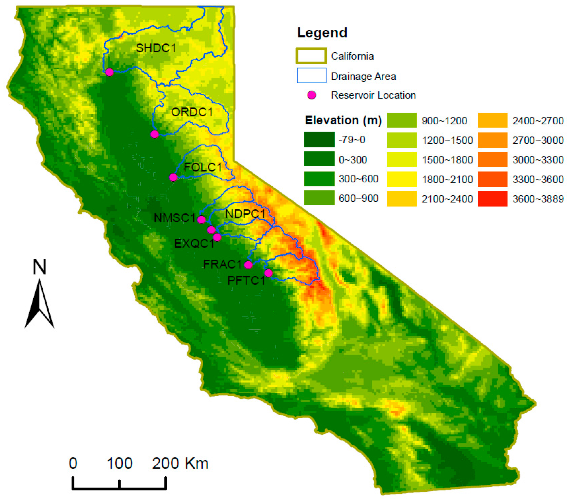
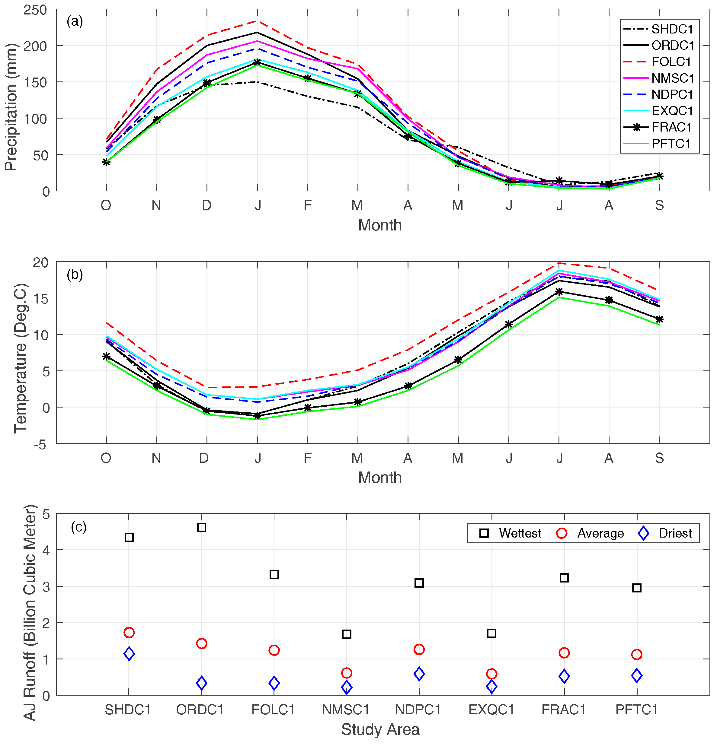
2.2. Study Watersheds and Datasets

This study focuses on eight Sierra Nevada watersheds draining into eight major reservoirs in California (

Table 1. Characteristics of study areas.

Reservoir Name	ID	Reservoir Capacity (109 m3)	Drainage Area (km2)	Annual Precipitation 1 (mm)	Annual Temperature 1 (°C)	Runoff
						April–July 1,2 (AJ, 109 m3)	Annual 1 (A, 109 m3)	Ratio (AJ/A)
Shasta Lake	SHDC1	5.61	16,630	936	8.0	2.23/1.83	7.30	0.31
Lake Oroville	ORDC1	4.36	9352	1174	7.9	1.88/1.53	5.13	0.37
Folsom Lake	FOLC1	1.21	4856	1294	10.6	1.47/1.27	3.33	0.44
New Melones Reservoir	NMSC1	2.96	2341	1160	8.6	0.78/0.68	1.40	0.55
Don Pedro Reservoir	NDPC1	2.50	3970	1093	8.4	1.51/1.40	2.43	0.62
Lake McClure	EXQC1	1.26	2686	987	8.9	0.77/0.66	1.23	0.62
Millerton Lake	FRAC1	0.64	4242	971	6.3	1.55/1.30	2.28	0.68
Pine Flat Reservoir	PFTC1	1.23	4105	913	5.8	1.52/1.19	2.14	0.71

¹ The tabulated values for those variables represent the 30-year (1981–2010) mean; ² The median value (second number) is presented along with the 30-year mean value.

; Figure 1). These reservoirs are selected for both practical and hydrological reasons. From the perspective of water supply, water from Sierra Nevada is a major source of the State’s surface water resources. Snowmelt from Sierra Nevada watersheds provides about one third of the State’s water supply in normal years. It also largely contributes to groundwater recharge particularly in the agriculture-intensive Central Valley areas. Those snow-impacted watersheds, in general, define hydrologic drought conditions statewide [63]. The social and economic value of reliable water supply forecasts in these areas is thus tremendous. Given its practical significance, consistent efforts have been invested in collecting and quality controlling of hydrological data (including the daily USGS streamflow data) in these areas. The streamflow data of these watersheds to be applied in verification is generally high in quality.

The aggregated capacity of these eight reservoirs accounts for about 42% of the total capacity of the State’s 154 major reservoirs. Out of the eight reservoirs, the largest two reservoirs (Shasta Lake and Oroville Lake) are the major water supply sources for the Central Valley Project (CVP) and State Water Project (SWP), respectively. The two projects collectively supply water to over 25 million Californians and about 15,000 km² of farmland annually on average. The three Northern reservoirs (Shasta Lake, Oroville Lake and Folsom Lake) have larger drainage areas, with the Shasta Lake on the top of the list (Table 1). For the others, the drainage area of the Millerton Lake is the largest, in spite of the fact that it has the smallest capacity. In general, the Folsom Lake drainage area is the wettest and warmest in terms of annual precipitation and temperature, respectively. In comparison, the Pine Flat Reservoir drainage area is the driest and coldest. With regard to runoff, the Shasta Lake receives the largest amount of it on both seasonal (April–July) and annual scales among eight study areas, while Lake McClure observes the least amount of it on both temporal scales. The ratio of April–July runoff over annual runoff, however, generally increases from north to south. This indicates the increasing dominance of snow contribution to the runoff in the southern Sierra watersheds in relatively higher elevations (Figure 1), given the fact that snowmelt is a major contribution to April–July runoff in the Sierra Nevada.

The study watersheds share a similar seasonality in precipitation (Figure 2a). All watersheds observe the majority (ranging from 79% at SHDC1 to 88% at PFTC1) of their annual precipitation in the wet season from November to April. All the watersheds receive the highest amount of precipitation in January. Average temperature values also display strong seasonality (Figure 2b), with low temperature in the winter (December–February) and high temperature in the summer (June–August). Overall, the Folsom Lake drainage area (FOLC1) is the warmest and also receives the highest amount of precipitation, while the Pine Flat Reservoir drainage area (PFTC1) tends to be the coldest and driest (in terms of precipitation). This observation is consistent with what has been shown in Table 1. In the study period (1985–2010), April–July streamflow runoff volumes at each study watershed varies largely from year to year (Figure 2c). The ratio of the highest (wettest) April–July runoff volume to the lowest (driest) value (over the study period) ranges from 3.8 (SHDC1) to 13.5 (ORDC1) with the median value being 6.5.

Retrospective forecasts (hindcasts) of streamflow at the outlet of these watersheds (Table 1; Figure 1) are generated with the HEFS for a ~26-year period (1985–2010) at 12Z each day. Inputs to the HEFS include raw ensemble mean (single-valued) precipitation and temperature forecasts from NCEP’s operational GEFS for the first 15 days and climatology from day 16 to 365. Each streamflow forecast has 60 members of 365 days in daily increments, representing a climatologic record from 1950 to 2009. The streamflow forecasts at each location are aggregated to the seasonal (April–July, AJ) scale. If the forecast is made later than 1 April when the April–July streamflow has been partially observed, the portion of observation (from 1 April until that forecast date) is added to the forecast. The combined value represents the forecast of the AJ streamflow for that forecast date, which is consistent with how the forecasts within the period from April to July are produced in real-time operations. To maintain consistency with the historical GEFS input data, streamflow observations in the same period (1985–2010) are used.

2.3. Verification Strategy and Metrics

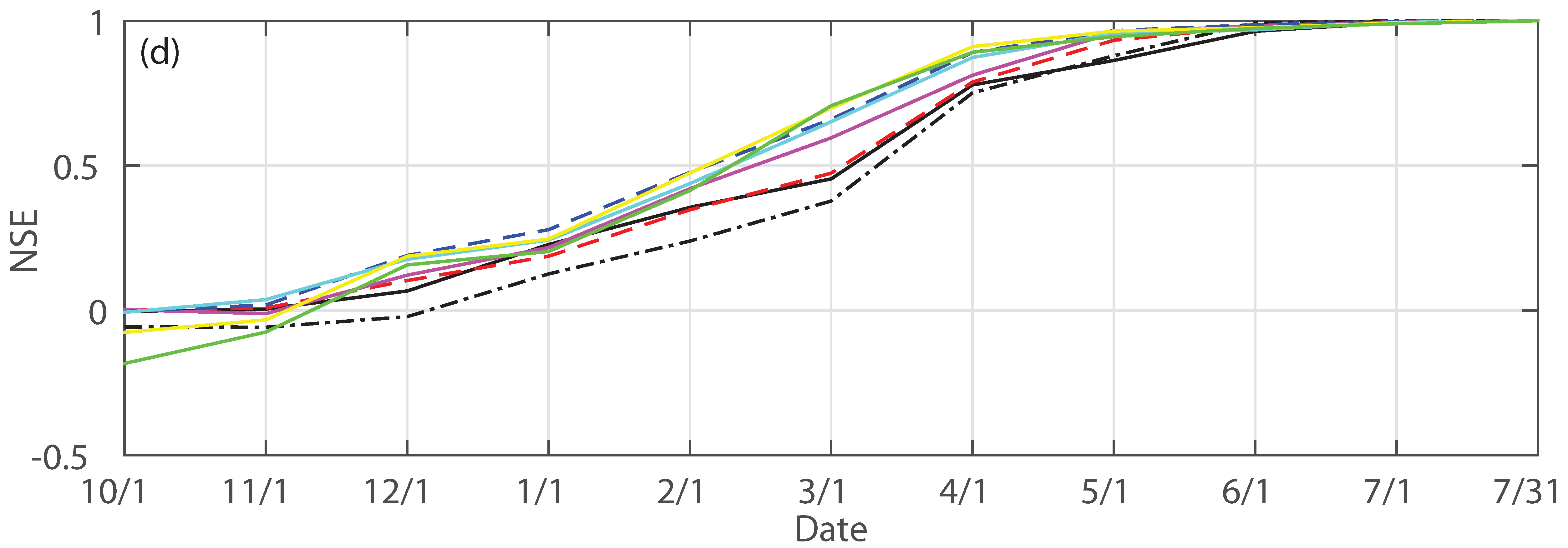
Based on our experience communicating ensemble forecast information to the users, forecast recipients are mostly concerned about the accuracy and correlation (with the observation) of the most probable forecast (ensemble median) as well as the reliability of specific percentile ranges of the ensemble forecasts. In spite of their advantageous properties and wide popularity in the research community, more sophisticated measures, including conditional statistics and categorical statistics [64] are often too difficult to understand for non-experts without significant and consistent training. Verification products are accordingly tailored in light of this observation, including (1) correlation plots showing the correlation between the median forecast and the observations; (2) scatter plots depicting the relationship between the median forecast and the observations; (3) percent error plots showing the bias of the median forecast from the observations; (4) box plots illustrating selected exceedance probability forecasts with observations; and (5) reliability histograms showing the forecast versus ideal frequencies in three percentile ranges of great interest to the users. The links to the verification products for the study watersheds are provided in Appendix A. This study summarizes the key features of these products and compares the forecast skills across different watersheds. A set of five metrics are employed for this purpose: Spearman’s rank correlation coefficient (R), percent bias (PB), skill score of mean absolute error (SSMAE), Nash–Sutcliffe efficiency (NSE), and containing ratio (CR). For a specific study watershed on a specific forecast date (ranging from 1 October to 31 July) these metrics are defined as follows:

$$R=1-\frac{6{{\displaystyle \sum }}_{i=1}^n{d_i}^2}{n\left(n^2-1\right)}$$

(1)

$$PB=\frac{{{\displaystyle \sum }}_{i=1}^n\left(f_i-o_i\right)}{{{\displaystyle \sum }}_{i=1}^n{o}_i}\times 100$$

(2)

$$SSMAE=1-\frac{{{\displaystyle \sum }}_{i=1}^n\left|f_i-o_i\right|}{{{\displaystyle \sum }}_{i=1}^n|o_i-\overline{o}|}$$

(3)

$$NSE=1-\frac{{{\displaystyle \sum }}_{i=1}^n{\left(f_i-o_i\right)}^2}{{{\displaystyle \sum }}_{i=1}^n{\left(o_i-\overline{o}\right)}^2}$$

(4)

$$CR=\frac{1}{n}{{\displaystyle \sum }}_{i=1}^n{I}_i\mathrm{where}{I}_i=\{\begin{array}{c}1,f_{low,i}\le o_i\le f_{up,i}\\ 0,otherwise\end{array}$$

(5)

where $d_i$ represents the difference between two ranks corresponding to the observation and median (or mean) forecast on AJ runoff volume, respectively; $n$ indicates the sample size, namely the number of years analyzed; $o_i$ and $f_i$ denote the individual observation and median (or mean) forecast on AJ runoff volume, respectively; $\overline{o}$ stands for the mean AJ runoff volume observation in the entire study period; $f_{low,i}$ and $f_{up,i}$ are the lower and upper bounds of a preset forecast exceedance probability range (e.g., between minimum and maximum forecasts), respectively. Those metrics quantify different aspects of the forecasts and collectively provide a comprehensive picture on the goodness of the forecasts. Specifically, the Spearman’s rank correlation estimates the strength of a monotonic relationship between the forecast and observation without any assumptions on the linearity or frequency distribution [65]. It ranges from −1 to 1 with a value of 1 indicating a perfect monotonic positive relationship. The percent bias is a direct measure of the forecast error divided by the observation. The mean absolute error skill score and the Nash–Sutcliffe efficiency are less or equal to 1. The former indicates the overall skill of the forecasts on all flow ranges. The latter reflects more on the skill of high flow forecasts due to the squared differences [66,67]. A value of 1 for both metrics indicates a perfect forecast; a value of zero implies that the forecast is no better than using the mean of observations as the forecast; a negative value denotes that mean observation is better than the forecast. The containing ratio is a measure of the reliability of the forecast in the context of showing how close the forecast frequency is to the observation frequency [68,69].

3. Results

3.1. Forecast Skill and Reliability

The rank correlation, percent bias, mean absolute error skill score and Nash–Sutcliffe efficiency between the most probable forecasts (i.e., median forecasts) and the corresponding observations for the study areas on the monthly scale (on the first day of every month) are determined (Figure 3). A general increasing tendency is evident in rank correlation (Figure 3a), mean absolute error skill score (Figure 3c), and Nash–Sutcliffe efficiency (Figure 3d) as forecast date approaches the end of the target forecast period (31 July). This is expected since the forcing data generally becomes more reliable when getting closer to the target forecast period (with more rainfall and snowfall accumulated throughout the wet season), while forcing uncertainty plays an important role in forecast skill, particularly when the lead time is long (months ahead). However, it is not the case for the percent bias (Figure 3b). As an example, the biases of the median forecasts issued on 1 February are generally larger than their counterparts of 1 January. This indicates that forcing is not the only factor that impacts forecast biases. Other factors, including dry and wet extremes as well as sample size, likely contribute to the bumpiness observed here. Those factors are investigated in Section 3.3 and Section 3.4.

Other than the general tendency, it is also clear that the forecast skill is limited before 1 January when the rank correlation (ranging from 0.46 at SHDC1 and FOLC1 to 0.62 at FRAC1 and PFTC1), mean absolute error skill score (ranging from 0.07 of FOLC1 to 0.16 of FRAC1 and PFTC1) and the Nash–Sutcliffe efficiency (ranging from 0.13 of SHDC1 to 0.28 of NDPC1) are small while the bias is significant (from −11.9% of PFTC1 to 1.6% of NDPC1). This is not surprising since the wettest month is typically January (Figure 2) for the study watersheds. The forecasts (before 1 January) on the April–July forcing do not contain the sufficiently accurate information on the wettest month plus the remaining part of the wet season (average climatology is used instead) and thus have limited skill. Comparing different study watersheds, forecasts for the Shasta drainage area (SHDC1) are the least skillful in terms of rank correlation, percent bias and Nash–Sutcliffe efficiency. On average, the forecasts for the three Northern study watersheds (SHDC1, ORDC1 and FOLC1) are less skillful than those five Southern study watersheds. These observations are also evident when looking at the metrics on the daily scale (Figure 4).

The median daily rank correlation (0.70) and Nash–Sutcliffe efficiency (0.39) of the forecasts for the Shasta drainage area are the smallest among all study watersheds (Figure 4). The median absolute mean error skill score (0.32) of SHDC1 is comparable to the smallest one (0.27) of the Oroville drainage area (ORDC1). In contrast, Lake McClure (EXQC1) and Millerton Lake (FRAC1) drainage areas have the highest median rank correlation (0.88); FRAC1 also has the highest median mean absolute error skill score (0.53) and Nash–Sutcliffe efficiency (0.70); Don Pedro Reservoir drainage area (NDPC1) has the smallest median bias (0.4%). Similar to those observed at the monthly scale (Figure 3), the forecasts for the five Southern study watersheds are more skillful in terms of rank correlation, mean absolute error skill score and Nash–Sutcliffe efficiency than those of the three Northern watersheds. The median values of these three metrics of the Southern (Northern) study watersheds are consistently above 0.84 (less than 0.81), 0.40 (less than 0.33) and 0.6 (less than 0.5), respectively. The median bias is generally negative for the study watersheds except for NDPC1. This dry bias likely stems from model calibration, which is explained in detail in Section 3.2.

In addition to looking at statistical metrics (Figure 3 and Figure 4), the median forecasts are also compared to the corresponding observations in a qualitative sense (Figure 5). It is evident that there is very little skill in the median forecasts for the fall and early winter months for all study locations. Similar to those observed previously (Figure 3), correlations between the median forecasts and the observations are generally low through 1 February. It is also evident that very large (small) April–July runoff years are under (over) forecast through 1 February. This is expected since precipitation forecast skill is fairly weak outside of about a week lead time; and climatology indicates that there can be quite large differences in precipitation amounts between dry and wet years for the February–April timeframe.

Aside from the median forecast, this study further examines other exceedance probability forecasts typically used in water resources planning, including the minimum, maximum, 90% exceedance probability and 10% exceedance probability. Specifically, the median containing ratios (CR) of (1) minimum forecast and maximum forecast (all members); (2) 90% forecast and 10% forecast (90% to 10% exceedance); (3) minimum forecast and forecast with 90% exceedance probability (<90% exceedance flow) and (4) forecast with 10% exceedance probability and maximum forecast (>10% exceedance flow) are determined for the forecasts from 1 October to 1 May (Figure 6). This period is selected since it is the period when the forecast reliability is of primary concern. Most major water resources planning and management plans are typically made prior to 1 May. Theoretically, 80% (CR = 0.8) of the observations should fall within the 90% and 10% exceedance forecast range which is represented by the dashed line in the plot. Ideally, the circles would fall directly on top of this line. This is the case for the Millerton Lake drainage area (FRAC1). However, other watersheds have smaller containing ratio values. Particularly, the more Northern watersheds from Shasta (SHDC1) through New Melones Reservoir (NMSC1) have a CR value ranging between 0.6 and 0.7. The dry forecasts (90% exceedance) and the wet forecasts (10% exceedance) should ideally fall along the solid black line (CR = 0.1). This is mainly true for the wet forecasts indicated by the plus symbol in the plot. However, the dry forecasts are slightly higher than the ideal value (0.1) for most watersheds. This illustrates that the forecast frequency of low April–July runoff is higher than the observed frequency. This issue is the main reason why the observed runoff volumes are not always contained within the ensemble spread. If they were, the squares would fall along the unity line (CR = 1) in the plot. However, the squares range from about 0.85 at Oroville (ORDC1) to near one for the Southern watersheds (EXQC1, FRAC1, and PFTC1). On average, the wet forecasts (with less than 10% exceedance probability) are generally reliable. The dry flows (with higher than 90% exceedance probability) are forecast more frequently than their actual frequency of occurrence. In contrast, the medium flows (90% to 10% exceedance) and all ranges (All Ensembles) of flows are forecast less frequently than their occurrence frequencies. Overall, the forecasts for the Southern watersheds (especially, EXQC1, FRAC1, and PFTC1) are more reliable than their counterparts of the Northern watersheds.

3.2. Mean versus Median Forecast

The median forecast tends to have negative bias in general (Figure 3b and Figure 4b). This is likely due to the fact that the rainfall-runoff models employed in generating these forecasts are calibrated to the mean (by minimizing the discrepancy between model simulation and observations) rather than the median, while the mean April–July runoff is typically higher than the median for the study watersheds (Table 1). The skill of the mean forecast is thus explored and compared to that of the median forecast. The bias of the mean forecast is first assessed (Figure 7). Except for the Pine Flat Reservoir (PFTC1) and the Shasta (SHDC1) drainage areas, the forecast bias at the monthly scale (Figure 7a) and the daily scale (Figure 7b) are generally positive (in contrast to negative biases in the median forecast). This implies that wet biases (over prediction) still exist in the calibrated models for most study watersheds. Bias values generally trend smaller the further into the water year. However, there are some oscillations of upward and downward bias from month to month, similar to those observed in the bias of the median forecast (Figure 3b). Generally, the bias ranges from roughly 10% to −5% starting in October, and tightening to ±5% by 1 April (Figure 7a), relatively smaller in absolute magnitude compared to that of the median forecasts (Figure 3b). This finding indicates that when bias is a major concern in decision-making, the mean forecast may be applied in lieu of the median forecast.

To gain a more complete picture on how the mean forecasts differ from the median forecasts, the discrepancies between four metrics (rank correlation, percent bias, mean absolute error skill score and Nash–Sutcliffe efficiency) for these two types of forecasts are examined (Figure 8). In general, the differences in rank correlation (Figure 8a) are small, particularly for the forecasts after 1 April when there are hardly any differences. There is no consensus among the study watersheds with regards to whether median forecasts or mean forecasts have a consistently higher rank correlation. It is a different case for percent bias. The discrepancies (median minus mean) are consistently negative across all study watersheds in every month (Figure 8b). The differences are the most significant in early forecast dates, with maximum values of −18.9%, −17.1%, −16.5% for 1 October, 1 November, and 1 December forecasts, respectively. The differences are insignificant after 1 April. In comparison, the mean absolute error skill score of the median forecast is generally higher than that of the mean forecast for all watersheds (Figure 8c), with a few exceptions in forecasts issued on 1 February and 1 April. There is no such consensus in the case of the Nash–Sutcliffe efficiency. For the most Northern (SHDC1) and most Southern (PFTC1) watersheds, the mean forecasts have higher efficiency values than the median forecasts through 1 April. For the other three Southern watersheds (NDPC1, EXQC1 and FRAC1), it is the opposite condition from 1 March to 1 May. The differences are negligible for forecasts issued on 1 June and 1 July.

3.3. Impact of Extreme Conditions

To explore the impact of extreme conditions on forecast skill and reliability, three different scenarios are considered with the forecasts in the wettest year (in terms of April–July runoff observation), the driest year, and in cases with both the wettest and driest years excluded, respectively (Figure 2c). Those five statistical metrics are calculated for these proposed scenarios and compared to their counterparts determined for the forecasts of the whole period (hereinafter reference scenario).

There are notable differences (proposed minus reference) in the rank correlation, mean absolute error skill score and Nash–Sutcliffe efficiency of these scenarios for all study watersheds (Figure 9a,c,d). In general, the differences become smaller towards the end of the forecast period. In the early phase of the forecast period (before 1 January), there is no consistent trend in the differences of these three skill scores from their counterparts determined in the reference scenario. However, since 1 January, the differences are all negative, reflecting that omitting the extreme years from the analysis period leads to reduced skill. Particularly, the largest difference normally occurs in the case when both the wettest and driest years are taken out. This highlights the importance of sample size (26, 25 and 24 for the scenarios with all years’ data, without the wettest (driest) year and without both the wettest and driest years, respectively) employed in calculating these metrics. In addition, the differences of the scenario with the driest year removed are generally the smallest, reflecting the relatively less important role of low flows in computing these metrics.

A general decreasing tendency in the differences (proposed minus reference) of the percent biases for all three scenarios through the forecast period is evident (Figure 9b). When not considering the driest year, the differences in percent bias are consistently negative while it is the opposite for the case when the wettest year is excluded. This is expected since, typically, the forecast system tends to under-forecast the wet extremes and over-forecast the dry extremes. Taking out the wettest (driest) year thus resembles the condition of removing a negative (positive) bias from the forecast, leading to over-prediction (under-prediction) in comparison to the case when forecasts in all years are accounted for. It is also worth noting that the differences of the scenario with both wettest and driest years removed are positive throughout the forecast period. This shows the dominance of the wet extreme over the dry extreme. The differences between the highest (wettest case) and mean April–July runoff measured by the amount of standard deviations range from 1.98 (PFTC1) to 2.45 (ORDC1). In contrast, in the driest case, the values vary from 1.09 (SHDC1) to 1.21 (FOLC1).

Similar findings are observed for these metrics on the daily scale. The median values of daily rank correlation, mean absolute error skill score and Nash–Sutcliffe efficiency (from 1 October to 31 July) of these three scenarios are generally less than their counterparts in the scenario when the whole study period is considered (differences ranging from −0.045 at SHDC1 to −0.002 at FRAC1 for R, from −0.044 at ORDC1 to −0.003 at FRAC1 in SSMAE, and from −0.074 at ORDC1 to −0.004 at NMSC1 in NSE). There are a few exceptions for the Nash–Sutcliffe efficiency of the scenario when the wettest year is excluded. In that scenario, the median Nash–Sutcliffe efficiency coefficients are higher than their counterparts determined in the reference scenario for Folsom (FOLC1, 2.3% higher), New Melones (NMSC1, 3.1% higher), and Pine Flat (PFTC1, 0.6% higher) areas, reflecting that forecasts on the wet extreme are relatively less skillful in these watersheds. There are also a few exceptions in the absolute mean error skill score. However, the differences are insignificant (range from 0.002 to 0.005). The pattern in precedent bias is also similar to that is observed on the monthly scale (Figure 9b). When the wettest year is not considered (in scenarios with only the wettest year and with both the wettest and driest years excluded), the percent biases are higher (ranging from 0.51% at ORDC1 to 3.2% at NMSC1); when the driest year is omitted, the percent biases are consistently smaller (ranging from −1.73% at ORDC1 to −0.30% at NMSC1 and NDPC1) across the study watersheds. Overall, the percent bias, along with rank correlation, mean absolute error skill score and Nash–Sutcliffe efficiency, exhibits high sensitivity to extreme conditions on both monthly and daily scales.

In addition to the median forecasts, different percentile ranges of the forecasts for those three scenarios are also assessed in terms of their coverage of the observations (containing ratio) relative to their counterparts determined in the reference scenario (Figure 10). There is no consistent trend in the change of the containing ratio for forecasts on all ranges of flows among all study watersheds (Figure 10a). Omitting the wettest year, driest year and both years from the analysis tends to have marginal influence on the containing ratios of the three most Southern watersheds (EXQC1, FRAC1 and PFTC1). In comparison, taking out both the wettest and driest years increases the containing ratios for the other five study watersheds. However, it is clear that the containing ratios of the 10% and 90% forecasts are higher for all watersheds in the scenarios when not considering the wettest year (Figure 10b), highlighting the difficulty of the 10th and 90th (percentile) forecasts in enveloping the wet extreme. The containing ratio of the dry forecasts (larger than 90% exceedance) generally becomes smaller (closer to the desirable value 0.1) when the driest year is excluded (Figure 10c), while the low flows are forecast to occur more frequently when all years are considered (Figure 6). It is also the case for the wet forecasts (less than 10% exceedance) when the wettest year is taken out (Figure 10d). This illustrates that the forecasts on the low (high) flows are more reliable in the case when the driest (wettest) year is not considered, highlighting the difficulty of the model in predicting the extremes.

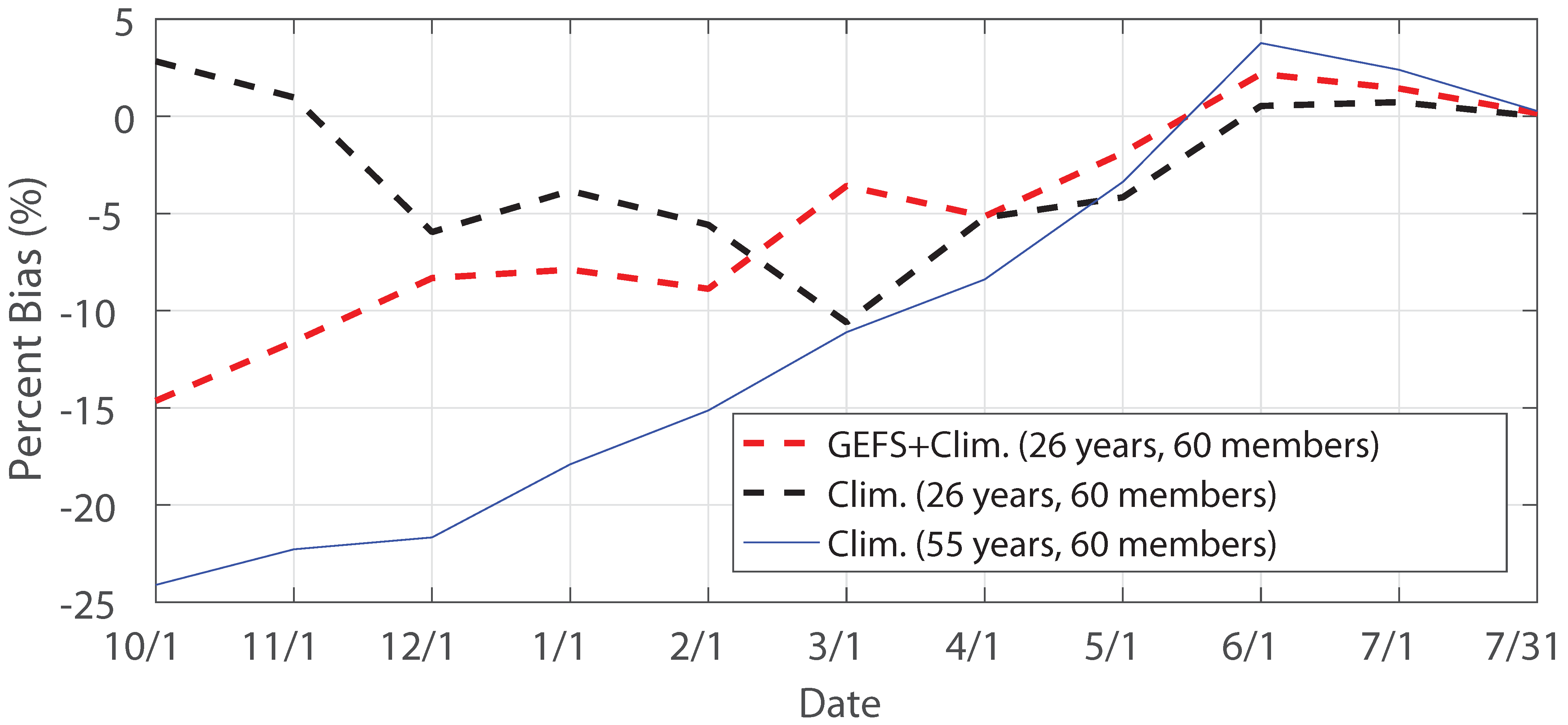
3.4. Impact of Forcing, Ensemble Size and Sample Size

To maintain consistency with the real-time operations, this study focuses on April–July streamflow reforecasts produced from the composite GEFS (with lead time up to 15 days) and climatology (from day 16 up to one year) forcing. Other forcing sources, including the pure climatology and the NCEP CFSv2 [70], can also be employed in generating water supply forecasts. To assess the impact of different forcing sources on the forecast results, this study explores the skill of the forecasts derived from pure climatology and CFSv2. Furthermore, in this study, the MEFP component of the HEFS is calibrated in the study period (1985–2010). However, it is applied to generate an ensemble of 60 traces of forcing reforecasts based on the climatology information from 1950 to 2009. This mismatch in calibration period and application period may have implications on the resulting streamflow forecasts. The study further examines the case when only 25 traces of forecasts are produced (based on climatology information in the study period only), to assess how the ensemble size impacts the forecast results. Additionally, the sample size (26) employed in this study is limited by the availability of archived GEFS data. A larger sample size would likely yield different forecast results.

To facilitate those analyses, four additional hindcasting runs are conducted. They are forced with (1) pure climatology from 1985 to 2010 (sample size: 26; ensemble member: 60); (2) CFSv2 from 1985 to 2010 (sample size: 26; ensemble member: 60); (3) GEFS (up to 15 days) and climatology from 1985 to 2010 (sample size: 26; ensemble member: 25) and (4) pure climatology from 1950 to 2010 (sample size: 61; ensemble member: 60), respectively. It is worth noting that the first and fourth scenarios require no MEFP calibration. The climatology is run through the hydrologic models directly to produce streamflow hindcasts in these cases. The third scenario shares the same MEFP parameters as the reference scenario (i.e., calibrated via archived GEFS and corresponding observations from 1985 to 2010). In the second scenario, the MEFP is calibrated using archived CFSv2 forecasts and corresponding observations. For the scenarios when GEFS or CFSv2 is considered (reference scenario along with the second and third scenario above), it should be highlighted that the verification is not independent as the GEFS and CFSv2 information are applied in both calibration and hindcasting processes. Ideally, the calibration period should not be overlapping with the hindcasting period, which would become feasible when a longer dataset is available (e.g., longer period of GEFS reforecasts). It should also be pointed out that CFSv2 hindcasts are only available once every five days in the study period. As such, the corresponding April–July streamflow reforecasts are only available at the same frequency. In the case when the forecast is not available on the first day of a month, the forecast on the closest date (typically one or two days off) is applied instead. Due to the fact that the focus of the study is not a comprehensive analysis of the impact of forcing, ensemble size and sample size on the forecasting skill, the analysis is conducted for only one study watershed (Folsom Lake, FOLC1) for demonstration purpose. A more comprehensive assessment of the impact of different forcing sources on the skill and reliability of corresponding streamflow forecasts has been conducted (not at the April–July seasonal scale specifically). The readers are referred to [61,62,71,72,73] for detailed analysis results.

There is a general increasing trend in rank correlation (R), mean absolute error skill score (SSMAE) and Nash–Sutcliffe efficiency (NSE) through the forecast period for all five (reference plus four proposed) scenarios investigated (Figure 11a,c,d). Before 1 January, as expected, forecast skill is limited in all scenarios (R < 0.5, SSMAE < 0.2 and NSE < 0.25) due to limited value of forcing forecasts with such a long lead time. After 1 May, those three metrics of different scenarios are almost identical to each other. This is not surprising since the precipitation amount from May through July is not significant (Figure 2). Snow melt runoff from snowpack accumulated during the wet season contributes largely to the streamflow in this period. As such, the impacts of difference forcing sources and different amounts of historical climate information (ensemble size) on forecast results are marginal. From 1 January to 1 April, overall, the median forecasts of the composite GEFS and climatology (reference) scenario (26 years, 60 members) are of the highest rank correlation in all scenarios. In comparison, the long-term climatology scenario (61 years, 60 members) has the highest SSMAE and the CFSv2 scenario has the highest NSE. Different from those three metrics, percent bias shows high sensitivity to different forcing sources and sample sizes before 1 June (Figure 11b). The oscillations in monthly percent bias are evident in each scenario. The biases are mostly negative for most scenarios. Overall, the CFSv2 scenario has the relatively smaller bias. The 25-member scenario has significantly higher biases before 1 February (largest bias −26% for the median forecast issued on 1 December) than the other four scenarios. From 1 March to 1 May, however, the long-term climatology (61-sample) scenario has the largest bias.

On the daily scale, the forecasts of the reference scenario are generally more skillful than other scenarios (

Table 2. Median metrics for daily median forecasts (1 October–31 July) of different scenarios for FOLC1.

Metrics	GEFS and Climatology		Climatology
	60 Members	25 Members	61 Samples	26 Samples
Rank Correlation	0.79	0.77	0.73	0.75
Percent Bias	−2.54%	−3.18%	−8.73%	−3.83%
Mean Absolute Error Skill Score	0.28	0.27	0.30	0.23
Nash-Sutcliffe Efficiency	0.47	0.46	0.42	0.39

). This scenario is with the highest median rank correlation and Nash–Sutcliffe efficiency along with the lowest percent bias. The forecasts of the GEFS and climatology with 25 members are secondary in general. The pure climatology scenario with 61 samples (1950–2010) has the lowest rank correlation but highest bias, while the pure climatology scenario with 26 samples (1985–2010) is with the lowest SSMAE and NSE. It is worth noting that since the CFSv2 forecasts are available once every five days, the corresponding scenario is not included in this analysis.

Despite the fact that the reference scenario provides generally the most skillful forecasts, those forecasts are not necessarily the most reliable (

Table 3. Median containing ratios of different forecasts (1 October–1 May) of different scenarios for FOLC1.

Range	GEFS and Climatology		Climatology
	60 Members	25 Members	61 Samples	26 Samples
Minimum–Maximum	0.84	0.80	0.82	0.88
90%–10% Exceedance	0.58	0.62	0.62	0.61
Minimum–90% Exceedance	0.27	0.27	0.20	0.27
10% Exceedance–Maximum	0.12	0.12	0.16	0.12

). In general, as in other scenarios, both the wet forecasts (less than 10% exceedance) and dry forecasts (higher than 90% exceedance) of the reference scenario are forecast more frequently than their actual occurring frequency. In contrast, the median flows (90% to 10% exceedance), are forecast less frequently than expected. Overall, forecasts (particularly wet forecasts) of the reference scenario are comparable to other scenarios in terms of reliability. However, relatively speaking, the pure climatology scenario with 61 samples (1950–2010) provides more reliable forecasts on median flows (90% to 10% exceedance) and low flows (larger than 90% exceedance); the pure climatology scenario with 26 samples has a higher containing ratio for the forecasts on all ranges of flows (minimum to maximum).

4. Discussion

Similar to the findings of previous studies assessing water supply forecasts produced from traditional regression-based approaches [42,45,47], this study indicates that the forecast skill of HEFS generally increases through the forecast period. Late in the forecast period (after May), the forecasts are highly satisfactory. From January to May, the forecasts are generally desirable. Early in the forecast period (before January), however, the skill is very limited. This is mainly due to the fact that the predictability in this period mostly derives from the seasonal climate forecasts (SCFs, in this case, the meteorological GEFS forecasts up to 15 days and climatology after that) which lack sufficient skill, though the HEFS has the capability of correcting the bias in meteorological forecasts. When the lead time becomes shorter (forecast date closer to 1 April), initial hydrologic conditions (IHCs, which are normally better predicted than SCFs since the study watersheds are all snow impacted and the hydrological models are well calibrated) increasingly contribute more to future flows compared to future climate inputs. Forecast skill and reliability increase accordingly since the predictability is more arising from the IHCs, particularly in snow-dominated watersheds (e.g., the Southern four watersheds as illustrated in Figure 3 and Figure 6). These observations are in line with previous studies [30,40]. Improvement of the forecast skill early in the forecast period would largely rely on improved skill of meteorological forecasts and climatic forecasts (i.e., SCFs). Given the fact that the hydrologic bias (associated with imperfect hydrologic model structure) is not addressed in HEFS hindcasting process, another area for improvement is utilizing streamflow observations to correct hydrologic bias. This may be achieved by assimilating streamflow observations into a hydrologic model to correct model states up to the forecast date in the hindcasting process [74,75]. However, given the long lead time (longer than three months) of the forecasts issued during this period, the skill of the forcing will override the skill of the hydrologic model in producing forecasts even when model states well reflect the reality at the forecast date. A more promising option is to post-process the forecasts via the post-processor component (EnsPost) of HEFS. The drawback is, however, that the performance of the EnsPost has never been evaluated for long-term forecast (including seasonal forecasts) yet it shows added value to short-term forecasts outside of CNRFC’s service area [62]. Nevertheless, in the case when the lead time is shorter (i.e., less than one month), both data assimilation and post-processing techniques hold great potential in improving HEFS forecast skill.

Despite the overall trend of decreasing bias through the forecast period, oscillations in the bias of median and mean forecasts for all study watersheds are evident at the monthly scale (Figure 3 and Figure 7). This bumpiness persists after removing the extreme year(s) in the calculation of bias (Figure 9), indicative of the marginal (if any) impact of extreme conditions on the variations in forecast bias. It is assumed that the small sample size (26; year 1985–2010) likely contributes to this bumpiness. A large sample size (61; year 1950–2010) is investigated for one watershed (Folsom; FOLC1) to verify this hypothesis. However, oscillation in monthly bias of the median forecast is also observed in this case (Figure 11), which implies that an even larger (than 61) sample size may be required to yield more statistically significant results. Notwithstanding this observation, similar hindcasting runs configured with different sample sizes are conducted for another study watershed (Pine Flat; PFTC1). These two watersheds have contrasting hydroclimatic characteristics (Figure 2), with FOLC1 being the wettest and hottest study watershed while PFTC1 being the coolest and one of the driest study watersheds. The bias of PFTC1 gradually decreases from −24.1% on 1 October to −3.4% on 1 May (Figure 12), different from the case of FOLC1. This indicates that the impact of a large sample size on variations in bias varies across study watersheds. Nonetheless, the oscillation observed in the forecasts produced with a large sample size for FOLC1 (and potentially other watersheds) warrants further investigation, which is part of our ongoing work.

On the dates when the traditional regression-based forecasts are available (typically on the first of every month from February to May with weekly updates in-between), the forecasts of HEFS are generally comparable to that of the regression-based approach in terms of skill. A recent study [47] examined the percent bias, mean absolute error skill score and Nash–Sutcliffe efficiency of regression-based forecasts on April–July runoff at 13 Sierra Nevada watersheds (including all study watersheds presented in this study except for the Shasta Lake drainage area). Their study reported that the absolute values of the median percent bias of forecasts issued on 1 April are generally around or above 10% (with the highest bias at around 20% for ORDC1). In comparison, for the current study, the percent bias of the median forecasts on 1 April ranges from −7.8% (PFTC1) to 0.3% (EXQC1) (Figure 3b). The median mean absolute error skill score (Nash–Sutcliffe efficiency) values for 13 watersheds in their study are close to 0.28 (0.45), 0.42 (0.58), 0.64 (0.83), and 0.77 (0.92) for forecasts issued on 1 February, 1 March, 1 April and 1 May, respectively. The corresponding median metric values at these four forecast dates in the current study are 0.27 (0.42), 0.41 (0.62), 0.63 (0.84), and 0.79 (0.95), respectively (Figure 3c,d). The HEFS has the advantages of being able to produce forecasts earlier in the water year (starting from 1 October rather than 1 February) on the daily basis over the regression-based approach. This is beneficial to water resources management practices that require long lead times and need forecast information updated more frequently. As an example, the initial water allocation decision of the State Water Project for the next year is typically made in late November or early December of the current year. In this case, the early forecasts provided by the HEFS can be useful (yet not highly skillful) in supporting the decision making. Additionally, during major precipitation events, particularly when the lead time is short (i.e., less than one month), the near real-time update frequency (daily) of HEFS is more appealing in the sense of incorporating the ongoing and GEFS-forecast storm information into the water supply forecasts.

5. Conclusions

The economic and social value of reliable water supply forecasting in California is tremendous. The State largely relies on water from Sierra Nevada as a major water supply source. This study evaluates seasonal (April–July) water supply forecasts produced from an innovative ensemble forecast system HEFS in eight Sierra Nevada watersheds. The specific objectives are to (1) assess the performance and limitations of the HEFS in producing seasonal water supply forecasts and (2) identify potential factors influencing the skill and reliability of the forecasts. Precipitation and temperature reforecasts during 1985–2010 from NCEP’s GEFS supplemented with climatology are employed as forcing to drive operational hydrological forecasting models in generating seasonal water supply forecasts. A set of statistical metrics are applied to verify the skill and reliability of these forecasts. The impact of extreme conditions on the forecasts is examined. The impact of forcing source, ensemble size and sample size on the results are also explored.

Results indicate that the forecast skill is limited when the lead time is long, over three months or before January) but increases through the forecast period. There is generally a negative bias in the most probable forecast (median forecast) for most study watersheds. When the mean forecast is investigated instead, the bias becomes mostly positive and generally smaller in magnitude. This implies that when bias is a major concern in decision making, the mean forecast may be utilized in favor of the median forecast. The forecasts, particularly the wet forecasts (with less than 10% exceedance probability) are reliable on average. The low April–July flows (with higher than 90% exceedance probability) are forecast more frequently than their actual occurrence frequency, while the medium April–July flows (90% to 10% exceedance) are forecast to occur less frequently. The forecast skill and reliability tend to be sensitive to extreme conditions. Particularly, the wet extremes show a more significant impact than the dry extremes and the high flows are more consistently influenced by extreme conditions across different study watersheds. Using different forcing data, including pure climatology and Climate Forecast System version 2 (CFSv2) shows no consistent improvement in the forecast skill and reliability; neither does using a longer (than the study period 1985–2010) period of record. This justifies the utilization of the current configuration (i.e., reference scenario) of HEFS in operational water supply forecasting. Comparing to traditional regression-based approaches, the HEFS provides forecasts having comparable skills but with the advantages of generating forecasts with longer lead time (starting from 1 October rather than 1 February) on a daily time step, which are beneficial for water resources management practices requiring long-lead forecast information with higher updated frequency (particularly during extreme events).

To summarize, this study identifies the strengths and weaknesses of the HEFS system in providing seasonal water supply forecasts. It has meaningful scientific and practical implications. From a scientific perspective, the system constitutes a significant step in the transition from traditional regression-based forecasting to ensemble forecasting in operations. As the skill of the meteorological (GEFS) forecasts continues to increase, the skill of the water supply forecasts in the late stage of the forecast period (e.g., after March) produced by the system is expected to increase accordingly. Moreover, as skill develops in longer-range climate (CFSv2) forecasts, that skill can be leveraged in this process as well. The skill of the system can also be improved by addressing the hydrologic uncertainty via data assimilation (of flow observations in particular) and post-processing techniques. Additionally, enhancements to the current system in forecasting extreme precipitation events would further improve its skill in seasonal water supply forecasting. From a practical standpoint, the system serves as a viable tool in providing critical information for water resources managers in terms of what to expect from the forecasts issued under what conditions (issue time, location, water year type) and how to tailor the forecasts to their needs. Particularly, they can capitalize on the ensemble nature of the products of this system and make timely and uncertainty-informed decisions in mitigating adverse impacts of hydroclimatic extremes and maximizing the reliability of water supply.

References

1. Twedt, T.M.; Burnash, R.J.C.; Ferral, R.L. Extended streamflow prediction during the California drought. In Proceedings of the 46th Annual Western Snow Conference, Otter Rock, OR, USA, 18–20 April 1978.
2. Krzysztofowicz, R. Optimal water supply planning based on seasonal runoff forecasts. Water Resour. Res. 1986, 22, 313–321. [Google Scholar] [CrossRef]
3. Krzysztofowicz, R. Expected utility, benefit, and loss criteria for seasonal water supply planning. Water Resour. Res. 1986, 22, 303–312. [Google Scholar] [CrossRef]
4. Yao, H.; Georgakakos, A. Assessment of Folsom Lake response to historical and potential future climate scenarios: 2. Reservoir management. J. Hydrol. 2001, 249, 176–196. [Google Scholar] [CrossRef]
5. Hamlet, A.F.; Huppert, D.; Lettenmaier, D.P. Economic value of long-lead streamflow forecasts for Columbia River hydropower. J. Water Resour. Plan. Manag. 2002, 128, 91–101. [Google Scholar] [CrossRef]
6. Maurer, E.P.; Lettenmaier, D.P. Potential effects of long-lead hydrologic predictability on Missouri River main-stem reservoirs. J. Clim. 2004, 17, 174–186. [Google Scholar] [CrossRef]
7. Brumbelow, K.; Georgakakos, A. Agricultural planning and irrigation management: The need for decision support. Clim. Rep. 2001, 1, 2–6. [Google Scholar]
8. Hayes, M.; Svoboda, M.; Le Comte, D.; Redmond, K.T.; Pasteris, P. Drought monitoring: New tools for the 21st century. In Drought and Water Crises: Science, Technology, and Management Issues; Wilhite, D.A., Ed.; CRC Press: Boca Raton, FL, USA, 2005; p. 53. [Google Scholar]
9. Smith, J.A.; Sheer, D.P.; Schaake, J. Use of hydrometeorological data in drought management: Potomac River basin case study. In Proceedings of the International Symposium on Hydrometeorology, Denver, CO, USA, 13–17 June 1982; pp. 347–354.
10. Sheer, D.P. Analyzing the risk of drought: The occoquan experience. J. Am. Water Works Assoc. 1980, 72, 246–253. [Google Scholar]
11. Zuzel, J.F.; Cox, L.M. A review of operational water supply forecasting techniques in areas of seasonal snowcover. In Proceedings of the 46th Annual Western Snow Conference, Otter Rock, OR, USA, 18–20 April 1978.
12. Huber, A.L.; Robertson, D.C. Regression models in water supply forecasting. In Proceedings of the 50th Annual Western Snow Conference, Reno, NV, USA, 19–23 April 1982.
13. Garen, D.C. Improved techniques in regression-based streamflow volume forecasting. J. Water Resour. Plan. Manag. 1992, 118, 654–670. [Google Scholar] [CrossRef]
14. Svensson, C. Seasonal river flow forecasts for the United Kingdom using persistence and historical analogues. Hydrol. Sci. J. 2016, 61, 19–35. [Google Scholar] [CrossRef]
15. Garen, D. ENSO indicators and long-range climate forecasts: Usage in seasonal streamflow volume forecasting in the western United States. Eos Trans. AGU 1998, 79, 45. [Google Scholar]
16. Moradkhani, H.; Meier, M. Long-lead water supply forecast using large-scale climate predictors and independent component analysis. J. Hydrol. Eng. 2010, 15, 744–762. [Google Scholar] [CrossRef]
17. Oubeidillah, A.A.; Tootle, G.A.; Moser, C.; Piechota, T.; Lamb, K. Upper Colorado River and Great Basin streamflow and snowpack forecasting using Pacific oceanic–atmospheric variability. J. Hydrol. 2011, 410, 169–177. [Google Scholar] [CrossRef]
18. Tootle, G.A.; Piechota, T.C. Suwannee River long range streamflow forecasts based on seasonal climate predictors. J. Am. Water Resour. Assoc. 2004, 40, 523–532. [Google Scholar] [CrossRef]
19. Piechota, T.C.; Chiew, F.H.; Dracup, J.A.; McMahon, T.A. Seasonal streamflow forecasting in eastern Australia and the El Niño–Southern Oscillation. Water Resour. Res. 1998, 34, 3035–3044. [Google Scholar] [CrossRef]
20. Tootle, G.A.; Singh, A.K.; Piechota, T.C.; Farnham, I. Long lead-time forecasting of US streamflow using partial least squares regression. J. Hydrol. Eng. 2007, 12, 442–451. [Google Scholar] [CrossRef]
21. Piechota, T.C.; Dracup, J.A. Long-range streamflow forecasting using El Niño-Southern Oscillation indicators. J. Hydrol. Eng. 1999, 4, 144–151. [Google Scholar] [CrossRef]
22. Grantz, K.; Rajagopalan, B.; Clark, M.; Zagona, E. A technique for incorporating large-scale climate information in basin-scale ensemble streamflow forecasts. Water Resour. Res. 2005, 41, W10410. [Google Scholar] [CrossRef]
23. Twedt, T.M.; Schaake, J.C., Jr.; Peck, E.L. National Weather Service extended streamflow prediction. In Proceedings of the 45th Annual Western Snow Conference, Albuquerque, NM, USA, 18–21 April 1977.
24. Day, G.N. Extended streamflow forecasting using NWSRFS. J. Water Resour. Plan. Manag. 1985, 111, 157–170. [Google Scholar] [CrossRef]
25. Hartman, R.K.; Henkel, A.F. Modernization of statistical procedures for water supply forecasting. In Proceedings of the 62nd Annual Western Snow Conference, Sante Fe, NM, USA, 18–21 April 1994.
26. Hamlet, A.F.; Lettenmaier, D.P. Columbia River streamflow forecasting based on ENSO and PDO climate signals. J. Water Resour. Plan. Manag. 1999, 125, 333–341. [Google Scholar] [CrossRef]
27. Souza Filho, F.A.; Lall, U. Seasonal to interannual ensemble streamflow forecasts for Ceara, Brazil: Applications of a multivariate, semiparametric algorithm. Water Resour. Res. 2003, 39, 1307. [Google Scholar] [CrossRef]
28. Najafi, M.R.; Moradkhani, H.; Piechota, T.C. Ensemble streamflow prediction: Climate signal weighting methods vs. Climate forecast system reanalysis. J. Hydrol. 2012, 442, 105–116. [Google Scholar] [CrossRef]
29. Wood, A.W.; Schaake, J.C. Correcting errors in streamflow forecast ensemble mean and spread. J. Hydrometeorol. 2008, 9, 132–148. [Google Scholar] [CrossRef]
30. Wood, A.W.; Kumar, A.; Lettenmaier, D.P. A retrospective assessment of National Centers for Environmental Prediction climate model–based ensemble hydrologic forecasting in the western United States. J. Geophys. Res. Atmos. 2005, 110, D04105. [Google Scholar] [CrossRef]
31. Wood, A.W.; Lettenmaier, D.P. A test bed for new seasonal hydrologic forecasting approaches in the western United States. Bull. Am. Meteorol. Soc. 2006, 87, 1699–1712. [Google Scholar] [CrossRef]
32. Wood, A.W.; Maurer, E.P.; Kumar, A.; Lettenmaier, D.P. Long-range experimental hydrologic forecasting for the eastern United States. J. Geophys. Res. Atmos. 2002, 107, 4429. [Google Scholar] [CrossRef]
33. DeChant, C.M.; Moradkhani, H. Toward a reliable prediction of seasonal forecast uncertainty: Addressing model and initial condition uncertainty with ensemble data assimilation and sequential bayesian combination. J. Hydrol. 2014, 519, 2967–2977. [Google Scholar] [CrossRef]
34. Tang, Q.; Lettenmaier, D.P. Use of satellite snow-cover data for streamflow prediction in the Feather River Basin, California. Int. J. Remote Sens. 2010, 31, 3745–3762. [Google Scholar] [CrossRef]
35. McGuire, M.; Wood, A.W.; Hamlet, A.F.; Lettenmaier, D.P. Use of satellite data for streamflow and reservoir storage forecasts in the Snake River Basin. J. Water Resour. Plan. Manag. 2006, 132, 97–110. [Google Scholar] [CrossRef]
36. DeChant, C.M.; Moradkhani, H. Improving the characterization of initial condition for ensemble streamflow prediction using data assimilation. Hydrol. Earth Syst. Sci. 2011, 15, 3399–3410. [Google Scholar] [CrossRef]
37. Li, H.; Luo, L.; Wood, E.F.; Schaake, J. The role of initial conditions and forcing uncertainties in seasonal hydrologic forecasting. J. Geophys. Res. Atmos. 2009, 114, D04114. [Google Scholar] [CrossRef]
38. Wood, A.W.; Lettenmaier, D.P. An ensemble approach for attribution of hydrologic prediction uncertainty. Geophys. Res. Lett. 2008, 35, L14401. [Google Scholar] [CrossRef]
39. Shi, X.; Wood, A.W.; Lettenmaier, D.P. How essential is hydrologic model calibration to seasonal streamflow forecasting? J. Hydrometeorol. 2008, 9, 1350–1363. [Google Scholar] [CrossRef]
40. Wood, A.W.; Hopson, T.; Newman, A.; Brekke, L.; Arnold, J.; Clark, M. Quantifying streamflow forecast skill elasticity to initial condition and climate prediction skill. J. Hydrometeorol. 2016, 17, 651–668. [Google Scholar] [CrossRef]
41. Rosenberg, E.A.; Wood, A.W.; Steinemann, A.C. Informing hydrometric network design for statistical seasonal streamflow forecasts. J. Hydrometeorol. 2013, 14, 1587–1604. [Google Scholar] [CrossRef]
42. Rosenberg, E.A.; Wood, A.W.; Steinemann, A.C. Statistical applications of physically based hydrologic models to seasonal streamflow forecasts. Water Resour. Res. 2011, 47, W00H14. [Google Scholar] [CrossRef]
43. Najafi, M.R.; Moradkhani, H. Ensemble combination of seasonal streamflow forecasts. J. Hydrol. Eng. 2015, 21, 04015043. [Google Scholar] [CrossRef]
44. He, M.; Gautam, M. Variability and trends in precipitation, temperature and drought indices in the State of California. Hydrology 2016, 3, 14. [Google Scholar] [CrossRef]
45. Pagano, T.; Garen, D.; Sorooshian, S. Evaluation of official western US seasonal water supply outlooks, 1922–2002. J. Hydrometeorol. 2004, 5, 896–909. [Google Scholar] [CrossRef]
46. Demargne, J.; Wu, L.; Regonda, S.K.; Brown, J.D.; Lee, H.; He, M.; Seo, D.-J.; Hartman, R.; Herr, H.D.; Fresch, M. The science of NOAA’s operational Hydrologic Ensemble Forecast Service. Bull. Am. Meteorol. Soc. 2014, 95, 79–98. [Google Scholar] [CrossRef]
47. Harrison, B.; Bales, R. Skill assessment of water supply forecasts for western Sierra Nevada watersheds. J. Hydrol. Eng. 2016, 21, 04016002. [Google Scholar] [CrossRef]
48. Demeritt, D.; Cloke, H.; Pappenberger, F.; Thielen, J.; Bartholmes, J.; Ramos, M.-H. Ensemble predictions and perceptions of risk, uncertainty, and error in flood forecasting. Environ. Hazards 2007, 7, 115–127. [Google Scholar] [CrossRef]
49. Cloke, H.; Pappenberger, F. Ensemble flood forecasting: A review. J. Hydrol. 2009, 375, 613–626. [Google Scholar] [CrossRef]
50. Demeritt, D.; Nobert, S.; Cloke, H.; Pappenberger, F. Challenges in communicating and using ensembles in operational flood forecasting. Meteorol. Appl. 2010, 17, 209–222. [Google Scholar] [CrossRef]
51. Ramos, M.H.; Mathevet, T.; Thielen, J.; Pappenberger, F. Communicating uncertainty in hydro-meteorological forecasts: Mission impossible? Meteorol. Appl. 2010, 17, 223–235. [Google Scholar] [CrossRef]
52. Pagano, T.C.; Wood, A.W.; Ramos, M.-H.; Cloke, H.L.; Pappenberger, F.; Clark, M.P.; Cranston, M.; Kavetski, D.; Mathevet, T.; Sorooshian, S. Challenges of operational river forecasting. J. Hydrometeorol. 2014, 15, 1692–1707. [Google Scholar] [CrossRef]
53. Hamill, T.M.; Bates, G.T.; Whitaker, J.S.; Murray, D.R.; Fiorino, M.; Galarneau, T.J., Jr.; Zhu, Y.; Lapenta, W. NOAA’s second-generation global medium-range ensemble reforecast dataset. Bull. Am. Meteorol. Soc. 2013, 94, 1553–1565. [Google Scholar] [CrossRef]
54. Wu, L.; Seo, D.-J.; Demargne, J.; Brown, J.D.; Cong, S.; Schaake, J. Generation of ensemble precipitation forecast from single-valued quantitative precipitation forecast for hydrologic ensemble prediction. J. Hydrol. 2011, 399, 281–298. [Google Scholar] [CrossRef]
55. Anderson, E.A. National Weather Service River Forecast System—Snow accumulation and ablation model. In Technical Memorandum NWS HYDRO-17; U.S. Dept. of Commerce, National Oceanic and Atmospheric Administration, National Weather Service: Silver Spring, MD, USA, 1973. [Google Scholar]
56. Burnash, R.J.; Ferral, R.L.; McGuire, R.A. A Generalized Streamflow Simulation System: Conceptual Modeling for Digital Computers; U.S. Department of Commerce, National Weather Service: Sacramento, CA, USA, 1973.
57. Duan, Q.; Sorooshian, S.; Gupta, V.K. Optimal use of the SCE-UA global optimization method for calibrating watershed models. J. Hydrol. 1994, 158, 265–284. [Google Scholar] [CrossRef]
58. Smith, M.B.; Laurine, D.P.; Koren, V.I.; Reed, S.M.; Zhang, Z. Hydrologic model calibration in the National Weather Service. In Calibration of Watershed Models; Duan, Q., Gupta, H., Sorooshian, S., Rousseau, A., Turcotte, R., Eds.; American Geophysical Union: Washington, DC, USA, 2003; pp. 133–152. [Google Scholar]
59. Kitzmiller, D.; Van Cooten, S.; Ding, F.; Howard, K.; Langston, C.; Zhang, J.; Moser, H.; Zhang, Y.; Gourley, J.J.; Kim, D. Evolving multisensor precipitation estimation methods: Their impacts on flow prediction using a distributed hydrologic model. J. Hydrometeorol. 2011, 12, 1414–1431. [Google Scholar] [CrossRef]
60. Seo, D.-J.; Herr, H.; Schaake, J. A statistical post-processor for accounting of hydrologic uncertainty in short-range ensemble streamflow prediction. Hydrol. Earth Syst. Sci. Discuss. 2006, 3, 1987–2035. [Google Scholar] [CrossRef]
61. Brown, J.D.; Wu, L.; He, M.; Regonda, S.; Lee, H.; Seo, D.-J. Verification of temperature, precipitation, and streamflow forecasts from the NOAA/NWS Hydrologic Ensemble Forecast Service (HEFS): 1. Experimental design and forcing verification. J. Hydrol. 2014, 519, 2869–2889. [Google Scholar] [CrossRef]
62. Brown, J.D.; He, M.; Regonda, S.; Wu, L.; Lee, H.; Seo, D.-J. Verification of temperature, precipitation, and streamflow forecasts from the NOAA/NWS Hydrologic Ensemble Forecast Service (HEFS): 2. Streamflow verification. J. Hydrol. 2014, 519, 2847–2868. [Google Scholar] [CrossRef]
63. Mao, Y.; Nijssen, B.; Lettenmaier, D.P. Is climate change implicated in the 2013–2014 California drought? A hydrologic perspective. Geophys. Res. Lett. 2015, 42, 2805–2813. [Google Scholar] [CrossRef]
64. Franz, K.J.; Hogue, T. Evaluating uncertainty estimates in hydrologic models: Borrowing measures from the forecast verification community. Hydrol. Earth Syst. Sci. 2011, 15, 3367. [Google Scholar] [CrossRef] [Green Version]
65. Lehmann, E.L.; D’abrera, H. Nonparametrics: Statistical Methods Based on Ranks; Holden-Day: San Francisco, CA, USA, 1975; p. 457. [Google Scholar]
66. Moriasi, D.N.; Arnold, J.G.; Van Liew, M.W.; Bingner, R.L.; Harmel, R.D.; Veith, T.L. Model evaluation guidelines for systematic quantification of accuracy in watershed simulations. Trans. ASABE 2007, 50, 885–900. [Google Scholar] [CrossRef]
67. Legates, D.R.; McCabe, G.J. Evaluating the use of “goodness-of-fit” measures in hydrologic and hydroclimatic model validation. Water Resour. Res. 1999, 35, 233–241. [Google Scholar] [CrossRef]
68. Xiong, L.; O’Connor, K.M. An empirical method to improve the prediction limits of the GLUE methodology in rainfall–runoff modeling. J. Hydrol. 2008, 349, 115–124. [Google Scholar] [CrossRef]
69. He, M.; Hogue, T.S.; Franz, K.J.; Margulis, S.A.; Vrugt, J.A. Characterizing parameter sensitivity and uncertainty for a snow model across hydroclimatic regimes. Adv. Water Resour. 2011, 34, 114–127. [Google Scholar] [CrossRef]
70. Saha, S.; Moorthi, S.; Wu, X.; Wang, J.; Nadiga, S.; Tripp, P.; Behringer, D.; Hou, Y.-T.; Chuang, H.-Y.; Iredell, M. The NCEP Climate Forecast System version 2. J. Clim. 2014, 27, 2185–2208. [Google Scholar] [CrossRef]
71. Brown, J. Verification of Temperature, Precipitation and Streamflow Forecasts from the Nws Hydrologic Ensemble Forecast Service (HEFS): Medium-Range Forecasts with Forcing Inputs from the Frozen Version of NCEP’s Global Forecast System; U.S. National Weather Service Office of Hydrologic Development: Silver Spring, MD, USA, 2013; p. 133.
72. Brown, J. Verification of Long-Range Temperature, Precipitation and Streamflow Forecasts from the Hydrologic Ensemble Forecast Service (HEFS) of the U.S. National Weather Service; U.S. National Weather Service Office of Hydrologic Development: Silver Spring, MD, USA, 2013; p. 128.
73. Brown, J. Verification of Temperature, Precipitation and Streamflow Forecasts from the Hydrologic Ensemble Forecast Service (HEFS) of the U.S. National Weather Service: An Evaluation of the Medium-Range Forecasts with Forcing Inputs from NCEP’s Global Ensemble Forecast System (GEFS) and a Comparison to the Frozen Version of NCEP’s Global Forecast System (GFS); U.S. National Weather Service Office of Hydrologic Development: Silver Spring, MD, USA, 2014; p. 139.
74. He, M.; Hogue, T.; Margulis, S.; Franz, K.J. An integrated uncertainty and ensemble-based data assimilation approach for improved operational streamflow predictions. Hydrol. Earth Syst. Sci. 2012, 16, 815–831. [Google Scholar] [CrossRef]
75. Franz, K.J.; Hogue, T.S.; Barik, M.; He, M. Assessment of swe data assimilation for ensemble streamflow predictions. J. Hydrol. 2014, 519, 2737–2746. [Google Scholar] [CrossRef]
Figure 1. Location map showing study reservoirs and their corresponding drainage areas.
Hydrology 03 00035 g001
Figure 2. (a) Mean monthly precipitation and (b) mean monthly temperature of the study areas for October (O), November (N), December (D), January (J), February (F), March (M), April (A), May (M), June (J), July (J), August (A), and September (S). Period of record is from water year 1949 to 2010; (c) April–July streamflow runoff volume (in billion m3) in the wettest, average, and driest years in the study period (1985–2010) for the study areas.
Hydrology 03 00035 g002
Figure 3. Statistical metrics of median forecasts of the April–July streamflow runoff volume at different issue dates (a) rank correlation; (b) percent bias (%); (c) mean absolute error skill score and (d) Nash–Sutcliffe efficiency for the study areas.
Hydrology 03 00035 g003aHydrology 03 00035 g003b
Figure 4. Boxplot of statistical metrics for median forecasts issued daily from 1 October to 31 July: (a) rank correlation; (b) percent bias (%); (c) mean absolute error skill score and (d) Nash–Sutcliffe efficiency for the study areas. The central mark on each box represents the median value; the edges of the boxes denote the 25th and 75th percentiles; the upper (lower) whisker is 1.5-times the interquartile range away from the top (bottom) of the box; the red crosses designate outliers.
Hydrology 03 00035 g004
Figure 5. Scatter plot of median forecasts versus observation on the monthly scale: (a) 1 October; (b) 1 November; (c) 1 December; (d) 1 January; (e) 1 February; (f) 1 March; (g) 1 April and (h) 1 May.
Hydrology 03 00035 g005
Figure 6. Median values of containing ratios from 1 October to 1 May of different categories of ensemble forecasts for the study watersheds. The dash line indicates the ideal containing ratio (0.8) for the 10% and 90% exceedance forecasts; the solid line represents the ideal containing ratio (0.1) for less than 90% exceedance and greater than 10% exceedance forecasts.
Hydrology 03 00035 g006
Figure 7. (a) Percent bias of mean forecasts at the monthly scale and (b) boxplot of percent bias of mean forecasts on the daily scale from 1 October to 31 July. The description of boxplot features is provided in Figure 4’s caption.
Hydrology 03 00035 g007
Figure 8. Differences between the statistical metrics of median forecasts and mean forecasts: (a) rank correlation; (b) percent bias (%); (c) mean absolute error skill score and (d) Nash–Sutcliffe efficiency on the monthly scale. X-axis shows the study area and Y-axis indicates the forecast issue date.
Hydrology 03 00035 g008
Figure 9. Median differences in the metrics of eight study watersheds: (a) rank correlation; (b) percent bias; (c) mean absolute error skill score and (d) Nash–Sutcliffe efficiency between the scenarios with the wettest year, driest year, wettest and driest years unconsidered and the scenario with all years considered.
Hydrology 03 00035 g009
Figure 10. Differences in median daily containing ratios of (a) maximum and minimum forecasts; (b) forecasts with 10% and 90% exceedance probabilities; (c) minimum forecast and forecast with 90% exceedance probability and (d) forecast with 10% exceedance probability and maximum forecast between the scenarios with the wettest year, driest year, wettest and driest years unconsidered and the scenario with all years considered.
Hydrology 03 00035 g010
Figure 11. Statistical metrics at the monthly scale: (a) rank correlation; (b) percent bias (%); (c) mean absolute error skill score and (d) Nash–Sutcliffe efficiency of median forecasts generated from five different scenarios for Folsom Lake drainage area (FOLC1).
Hydrology 03 00035 g011
Figure 12. Percent bias (%) of the median forecasts from three different scenarios for PFTC1.
Hydrology 03 00035 g012