Infilling Monthly Rain Gauge Data Gaps with Satellite Estimates for ASAL of Kenya

Abstract

Design and operation of water resources management systems in sub-Saharan Africa suffer from inadequate observation data. Long running uninterrupted time series of data are often not available for water resource planning. Incomplete datasets with missing gaps is a challenge for users of the data. Inadequate data compromise results of analyses leading to wrong inference and conclusions of scientific assessments and research. Infilling of missing sections of data is necessary prior to the practical use of hydrometeorological time series. This paper proposes the use of Tropical Rainfall Measuring Mission satellite data as a viable alternate source of infill for missing rain gauge records. The least square regression method, using satellite-based estimates of rainfall was tested to fill in the missing data for 153 data points at nine rain gauge stations in Machakos, Makueni and the Kitui region of Kenya. Results suggest that the satellite rainfall estimates can be used as an alternative data source for rainfall series where the missing data gaps are large. The infilled data series were used in the development of monitoring, forecasting and drought early warning for Arid and Semi-Arid Lands (ASAL) in Kenya.

1. Introduction

As in other Arid and Semi-Arid Lands (ASAL) of Kenya, climatic variations have been experienced over the years in the south eastern lowlands of Kitui, Machakos and Makueni counties. The typical approach to gaining understanding of climate variability starts with the acquisition of historical data. For rainfall, historical data provide necessary information about accumulated amounts in both time and space and form the basis for fitting and testing stochastic data-based distribution models. When historical data is unavailable in a region, or available data is inaccurate or incomplete in a spatial or temporal sense, geophysical models can be used to ‘fill in’ the missing values [1]. According to Collischonn et al., [1], areal rainfall estimated by rain gauges exhibits a great deal of uncertainty where the rain gauge network is sparse. This problem is related to the differences in distribution of rain gauges around the region. This situation also affects the quality of data. This paper suggests a method of improving rain gauge-based rainfall measurement datasets through infilling missing gaps using remotely sensed rainfall estimates.

Generally, in operation and model validation of meteorological data, surface observations are considered to be “the truth” [2]. Analysis of climatic systems require availability of data forming a complete and homogeneous series to enable generalised deduction and inference from results [3]. This is especially important for those approaches that use statistical techniques based on the estimation of covariance matrices, e.g., the principal component, cluster, or discriminant analysis, the canonical correlation method, and the method of multiple linear regressions [4]. In Africa in general and Kenya in particular, incomplete datasets of climatic variables are frequent with the ensuing appearance of gaps in the measurement series [5]. The existence of missing values in the data series affects the variable estimation from the series [6], and the output of multivariate analysis techniques [7].

Hydrometeorological data analysis such as drought assessment and forecast benefit from a complete dataset [8]. A possible way of minimizing the influence of missing data is to rebuild the series, filling in the gaps with estimated values. Various methods for the estimation of missing values in climatological series exist. Bareither et al., [2], evaluated the influence of replacing missing meteorological data with estimates on hydrologic predictions for a water balance model in a semiarid climate. According to Bareither et al., [2], surrogate data technique yields modest predictions of annual water percolation that are statistically similar to percolation predicted using actual data. Aly et al., [9], evaluated deterministic and stochastic interpolation methods to fill gaps in daily precipitation records.

The simplest and more direct methods of data extension take into account the data of the series that is being filled. The arithmetic mean method substitutes missing values by the series mean value of the series. Thus, although the average value of the series is not altered, its variance is reduced and thus the method rendered inefficient to address highly variable climatic quantities, such as precipitation [10]. Other methods include the linear interpolation method and the first differences method both of which are particularly appropriate for small temporal scales and variables with high autocorrelation [10].

Methodologies which use information from different sites other than the station with missing data (target station) have also been developed. These methods take into account the spatial variability of the measured variable, ignoring the temporal information in long-time series [11]. Such methods include the closest station method [12], the simple arithmetic averaging method; the inverse distance method, the single best estimator method, and the normal ratio method. These methods generally under and/or overestimate the high and low extremes, respectively [13].

Another important set of approaches for gap filling in climatological series is regression methods. These methods are based on relationship techniques of the temporal series of the variable under consideration [14]. They take into account the station’s ‘history’ and its climatic characteristics without consideration of spatial dependence of the variables. Uncertainty in climate parameters however originate from its stochastic nature [15], and its magnitude depends on other environmental factors, intrinsic on the recorded value [16]. Spatial characteristics of the uncertainty enters the records through the procedure for stations selection [17] when stations other than the target station are considered. The procedures followed for the selection of neighbour stations in the regressive methods utilizes relative weighting, enabling differentiation of analysis from one station to another. The regression methods have the advantage of robustness when dealing with extreme events or local effects [18]. This paper utilizes the least square regression method for the estimation of missing data in a monthly precipitation dataset taking into account the measurement uncertainty. The paper addresses the question of whether remote sensing rainfall estimates over a region can be used for infilling missing data in the time series of rain gauge-based data. The Tropical Rainfall Measuring Mission (TRMM) satellite datasets was selected on the basis of its good prior performance in estimating rainfall in East Africa [19,20] in particular and in many parts of the tropics [21] in general.

Errors occurring due to rain gauge measurements are fairly well understood [22], and so, except for their limited coverage, they are ideal for checking satellite estimates [22]. The use of satellite estimates to fill rain gauge measurements on the other hand however raises errors due to the space-time differences of the two measurement methods. While rain gauge measurements are point (tens of centimetres in diameter) estimates, satellite measurements are a good attempt to measure rain amounts over areas many kilometres in diameter around a point (rain gauge position). Bell and Kundu [22] investigated the “noisiness” in the comparisons of satellite and rain gauge estimates given the very different observational characteristics of the two. Bell and Kundu [22] observed that the satellite measurements catches glimpses of large areas at infrequent intervals, whereas rain gauges record what happens in small areas continuously. Panet et al., [23] alluded that the presence of non-negligible errors in satellite rainfall estimation presents a hurdle to fully implement the product for wide ranges of hydrologic applications. Gebregiorgis and Hossain [24], however, indicated that the quantitative picture of satellite precipitation error over ungauged regions can be effectively discerned. The paper makes consideration of the space–time scale difference of rainfall estimates based on the point rain gauge measurements and satellite-based estimates.

Rain gauge data series in Machakos, Makueni and Kitui counties of Kenya for the period 2001–2011 has long running data gaps of over two years. These data gaps however form less than 5% of the total length of existing the data for most of the rain gauge stations in the region. The data series are therefore worth consideration for infilling in view of their importance to connect the historical rainfall analysis and the current rainfall situation [25]. The purpose of this paper is to proposes the use of TRMM data as a viable alternate source of infill for missing rain gauge records. The method of infill utilizes linear regression relationships and make use the records of a reference station which cover the period of interest. The paper demonstrates the use of satellite rainfall estimate data for extending rain gauge records by infilling missing gaps in a rainfall data series. The method adapts the MOVE.2 approach [26] in a variation of linear regression equations [27], which ensure preservation of characteristics of the statistical parameters (mean, variance and extreme value statistics), of the infilled data series. The Gamma distribution with shape parameter α and scale parameter β is often assumed to be suitable for distributions of precipitation events [28]. This distribution has been proven to be effective for the analysis of precipitation data in previous studies [29]. The gamma distribution was used in this study to confirm that the infilled data did not alter the parameters of the original series.

In this study, an attempt was made to infill missing monthly rainfall data for 153 missing data points for 9 rain gauge stations in Machakos, Makueni and Kitui counties of Kenya. This paper is organized as follows; first, this introduction giving the background, the problem, the objectives and rationale of the study. The materials and methods used to address the research question and related formulation of proposed solution, and technical details, such as approaches for estimation of infilling model, are detailed in Section 2. The results of the infilling process and evaluation of model achievements in infilling datasets and related statistical test are discussed in Section 3 followed by summary and concluding remarks in Section 4.

2. Materials and Methods

This study was carried out in Machakos Makueni and Kitui Counties of Kenya. The study area is located in the arid and semi-arid regions of the country. The area lies between Latitude 00°03′ and 3°00′ and Longitudes 36°45′ degrees 39°12′ (Figure 1). The area receives rains twice a year, with the main rains season occurring in October to December and the lesser rains season occurring in March to May. The annual rainfall ranges from 500 mm in the low moorland areas to 1500 mm in the sub-humid hilltops. The seasonal rainfall is highly variable, erratic and unreliable.

2.1. DATA

The data used in this study is of secondary nature comprising of rainfall elements measured on rain gauge instruments in the study area and satellite based rainfall estimates. The rain gauge data series comprised of monthly records for the period 1961–2011 for the different stations. Only rain gauges with missing data gaps were considered in this study. The rain gauge data series used comprised of records for the period 1961–2011 for the different stations.

Table 1. Locations of the rain gauges, corresponding grid point for Tropical Rainfall Measuring Mission (TRMM) data extraction, distance between rain gauge location and grid point data, the number and Proportion of data points of missing record and the period of missing data.

Station Name	Station Identifier Number	Station Location		Location of for TRMM Pixel Centre		Distance (km) between Rain Gauge and TRMM Grid Point	Number of Missing Data Points (1961–2011)	Percentage (%) of Missing Data of Total Data-Set (1961–2011)	Period of Missing Data Points
		Latitude (Degrees)	Longitude (Degrees)	Latitude (Degrees)	Longitude (Degrees)
Kambi ya Mawe	9137075	−1.85	37.6667	−1.75	37.75	0.520	12	1.96	Jan 2011–Dec 2011
Mutonguni	9137094	−1.28	37.9833	−1.0	38	0.75	24	3.92	Jan 2010–Dec 2011
Kitui	9137095	−1.22	37.59	−1.25	38	0.23	24	3.92	Jan 2009–Dec 2010
Mutomo	9138001	−1.85	38.2	−1.75	38.25	0.45	12	1.96	Jul–Nov 2010
Kisasi	9138037	−1.5333	38.0167	−1.5	38	0.15	30	4.9	Jul 2008–Dec 2009 and Jan–Dec 2011
Lukenya	9137046	−1.5333	37.6167	−1.5	37.5	0.49	29	4.73	Jan 2010–May 2011
Matungulu	9137040	−1.2667	37.35	−1.25	37.25	0.41	29	4.73	Jan–Dec 2011
Matiliku	9137028	−1.95	37.533	−2.0	37.5	0.20	19	3.10	Jan–Jul 2009
Mutito Forest	9138040	−1.13	38.11	−1.0	38.25	0.65	26	4.24	Nov 2010–Dec 2011

below shows the length of the rain gauge data series used in the study. TRMM is a joint mission of the U.S. National Aeronautics and Space Administration (NASA) and the Japan Aerospace Exploration Agency (JAXA), designed to monitor and study tropical rainfall [31]. TRMM has a data coverage area, ranging from latitudes 50° S to 50° N, and a spatial resolution (0.25° × 0.25°). The TRMM rainfall estimates have more reliable data than those obtained from other satellites [32]. The TRMM data series used in this study comprised of records for the period 1998–2011.

2.2. Data Analysis Approach

Two types or techniques of data analysis were considered to achieve the objectives of this study; correlation analysis and the least squares regression method. Data from closest TRMM grid point were compared against each respective rain gauge.

TRMM data from the chosen grid point was used to compare with the corresponding observed rain gauge data. Correlation analysis was used for comparison of the rain gauge and TRMM data fields to confirm relationship of the two data series.

Table 1 shows the locations of the rain gauges matched with the corresponding grid point at which monthly TRMM data was extracted, the estimated distance between rain gauge location and grid point data, the number of data points of missing record and the period of missing rain gauge data. The datasets of the rain gauges had large continuous gaps of missing data for period 2008–2011.

The least square regression method was used to translate estimates of rainfall values donated by the TRMM data series into rainfall values for infilling into the rain gauge series. The viability of the TRMM rainfall data to infill rain gauge missing data gaps was first evaluated through comparison with rain gauge data for the periods in which the rain gauge datasets were complete. Descriptive statistics of station rainfall was calculated for all the TRMM cells and corresponding rain gauge stations, and compared in monthly intervals. Scatter plots of the rain gauge data and TRMM were plotted to confirm the versatility of TRMM data to infill the rain gauge data.

2.3. Methods of Infilling Rain-Gauge Data

A variation of the linear regression method as employed by Krug et al. [33] was used in this study. The method considers that if records for a normal climatological period of 30-years are incomplete for a desired station, then the records are extended by correlation with a nearby station using Equation (1).

Y₁ = y_s + (b)(x₁ − x_s)

(1)

where

• y₁ = the estimated value for the missing gap rain gauge data for the respective month.
• y_s = the mean value for the respective month for TRMM dataset for the period of record 14 years (1998–2011).
• b = the slope of the regression line between the concurrent (1998–2011), mean value at the rain gauge station and TRMM.
• x₁ = the 30-year (climatological standard 1971–2000) mean value for the monthly rain gauge data.
• x_s = the mean value for the rain gauge station for the concurrent period with the TRMM.

TRMM datasets were used to estimate monthly values of rain gauge records to fill the gaps. The TRMM data at respective grid point was used as reference for corresponding rain gauge as indicated in Table 1. In this approach, the least squares regression was used in an extension method following a linear form (y = bx + c), but that the coefficient “b” and constant “c” were set not to minimize squared errors, but rather to maintain the sample mean and the variance according to Hirsch [26]. Two such linear equations that preserve the sample mean and variance are given in Hirsch [26]. These equations are labelled: “Maintenance of Variance Extension, Type I” (MOVE.1) and “Type 2” (MOVE.2).

Hirsch [34] evaluated MOVE.1 for streamflow data extension methods and Parrett and Johnson [35] utilized MOVE.1 for extending streamflow gaging data in eastern Montana over a fifty year period of record. Alley and Burns [36] and Hirsch [26] evaluated MOVE.1, and MOVE.2, for streamflow data extension using least squares linear regression and linear regression plus white-noise based on criteria of sample mean and variance maintenance. These works from the literature suggest that MOVE.2 is the most effective infilling method in preserving the mean, variance, and extreme order statistics of a baseline data. As such MOVE.2 was used in this study to extend the rain gauge data using TRMM monthly rainfall data.

2.3.1. MOVE.2 Method

Missing rain gauge data were infilled using related TRMM data following the MOVE.2 model. The TRMM values are denoted as “X(I)” where “I” is an index of time (month). The rain gauge data values were denoted as “Y(I)”. The events for the two sequences are represented as:

X(1), .........., X(N1), X(N1 + 1),............................., X(N1 + N2)
Y(1),.........................,Y(N1)

where “N1” represents the number of rain gauge/TRMM data values used to make the regression equation. When “N1” is less than 10, there is not enough known TRMM data to build a regression relationship (since TRMM data records commences at 1998). “N2” represents the number of missing data gaps in the series. When “N2” is equal to 1, there is only one missing data gap. “N1 + N2”represents the total number of values in the data set. The following notations identify the different parts of the two series.

X = x(1),..................., X(N1), x(N1 + 1),........................., X(N1 + N2)

(2)

X1 = x(1),.............., X(N1)

(3)

X2 = x(N1 + 1),................, X(N1 + N2)

(4)

Y1 = y(1),..............................., Y(N1)

(5)

It is not necessary for the two sequences to begin or end simultaneously, nor for the observations be consecutive [26]. The MOVE.2 infilling equation yielding an estimate for the missing rain gauge data, denoted as “[yN(I)]”, is given by the relationships in Equations (6)–(9) as derived by Hirsch [26].

$$\mathrm{y}\prime \left(\mathrm{i}\right)=\mathrm{m}\prime \left(\mathrm{y}1\right)+\frac{\mathrm{S}\prime \left(\mathrm{y}\right)}{\mathrm{S}\left(\mathrm{x}\right)}\left[\mathrm{x}\left(\mathrm{i}\right)-\mathrm{m}\left(\mathrm{x}\right)\right]$$

(6)

$$\mathrm{m}\prime \left(\mathrm{y}\right)=\mathrm{m}\left(\mathrm{y}1\right)+\frac{\mathrm{N}2}{\mathrm{N}1+\mathrm{N}2}r\frac{\mathrm{S}\left(\mathrm{y}1\right)}{\mathrm{S}\left(\mathrm{x}2\right)}\left[\mathrm{m}\left(\mathrm{x}2\right)-\mathrm{m}\left(\mathrm{x}1\right)\right]$$

(7)

$$\mathrm{S}\prime \left(\mathrm{y}\right)=\frac{1}{\mathrm{N}1+\mathrm{N}2-1}[(\mathrm{N}1-1)]{\mathrm{S}}^2(\mathrm{y}1)+[(\mathrm{N}2-1)]{\mathrm{r}}^2\frac{{\mathrm{S}}^2\left(\mathrm{y}1\right)}{{\mathrm{S}}^2\left(\mathrm{x}1\right)}{\mathrm{S}}^2\left(\mathrm{x}2\right)+(\mathrm{N}2-1)\stackrel{`}{a}(1-r^2){\mathrm{S}}^2\left(\mathrm{y}1\right)+\frac{N1N2}{N1+N2}{r}^2\frac{{\mathrm{S}}^2\left(\mathrm{y}1\right)}{{\mathrm{S}}^2\left(\mathrm{x}1\right)}[{(\mathrm{m}\left(\mathrm{x}2\right)-\mathrm{m}\left(\mathrm{x}1\right))}^2]$$

(8)

$$\stackrel{`}{a}=\frac{N2\left(N1-4\right)\left(N1-1\right)}{\left(N2-1\right)(N1-3)\left(N1-2\right)}$$

(9)

where “m()” and “s²()” represent the mean and variance of the series in the parentheses respectively; “r” represents the product moment correlation coefficient of “x1” and “y1”.

Thus, in the MOVE.2 method, the mean and variance estimates for “x” are based on all “N1 + N2” observations, and the mean and variance estimates for “y” (i.e., “mN(y)” and “SN2(y)” respectively) are based on the historical values of “y” and on information transferred from the “x” sequence of data. à is a coefficient.

2.3.2. Evaluation of Infilled Data Series

Evaluation was done to examine the extent to which the MOVE.2 method would yield correct values of estimated rain gauge data to infill gaps on repeated trials. Given that the MOVE.2 approach was used in the study to infill long running data gaps, it was necessary to create long running gaps for purpose of the evaluation of the method. The procedure involved removing 12 successive points from the rain gauge data series to create running gaps in the rain gauge series. The gaps were created for each station for the respective years commencing 2007–2011. The months which data was removed was the months which did not have a gap in the original unfilled rain gauge series. If one month had gaps in the original rain gauge data series, this month was not included in this part of analysis.

For each of the months with removed data, a value was computed following the MOVE.2 approach and the same was used to fill the created gap. The months whose data was removed were then replaced with MOVE.2 data series and the series was used in test of reliability. The procedure to remove the data for the respective months was done in steps so that not any more than one year (12 months), were removed at the same time, but each year was removed with successive replacement of the same data to be used in computing MOVE.2 values of next removed year.

2.3.3. Jacknife Sampling Approach

A jackknifing sampling approach was used to evaluate the effectiveness of the MOVE.2 approach to infill rain gauge data gaps. In this simulation, the actual rain gauge data was compared with corresponding TRMM-MOVE.2 values for the respective periods. Thus, in this approach, it was easy to compare performance of imputation methods. The following notation was used in a sums of squares equation:

Y_ijk = is the rainfall value measured on a rain gauge for the ith month, jth year and kth station, and is an element in the rain gauge dataset of the station within the period 1998–2011. For purpose of evaluation, Y_ijk was removed from the dataset and replaced with an estimated value Z_ijk.

Therefore,

$$\overline{Y}=\frac{1}{N1}{\displaystyle \sum }_1^n{\mathrm{Y}}_{ijk}$$

(10)

is the average of the rainfall value measured on a rain gauge for the ith month, jth year and kth station and

$$\overline{Y_{.j.}}=\frac{1}{N1}{\displaystyle \sum }_{k=1}^n{\overline{\mathrm{Y}}}_{.jk}$$

(11)

tracks the average change across all the data years as the MOVE.2 model is simulated to estimate the values of removed rainfall values of the respective rain gauge with subsequent replacement.

Z_ijk is the MOVE.2 estimated value of rainfall for the ith month, jth year and kth station which was used to infill the data gap created by removing Y_ijk, Z_ijk is thus an element in the TRMM-MOVE.2 imputed rainfall series.

Likewise,

$$\overline{Z}=\frac{1}{N1}{\displaystyle \sum }_1^n{\mathrm{Z}}_{ijk}$$

(12)

is the average value of the MOVE.2 estimated rainfall for the ith month, jth year and kth station which was used to infill the data gap created by removing Y_ijk, and

$$\overline{{\overline{Z}}_{.j.}}=\frac{1}{N1}{\displaystyle \sum }_{k=1}^n{\overline{\mathrm{Z}}}_{.jk}$$

(13)

tracks the average change across all the data years as the MOVE.2 values are simulated and added to the series of the removed rainfall values of the respective rain gauge with subsequent replacement.

2.3.4. Evaluation of Errors in the MOVE.2 Estimates

An evaluation of the suitability of the MOVE.2 values for infilling the rain gauge data gaps was done. The evaluation compared samples of the original rain gauge values with MOVE.2 values for the respective sample areas. The evaluation followed 3 steps as follows: first a visual inspection and comparison of non-parametric characteristics of the infilled series against original series was done. The non-parametric comparison considered the descriptive statistics such as median, skewness, kurtosis, minimum and maximum values with due consideration of the influence of the statistics in the distribution of the data sets.

The second step in the evaluation considered the effect of random errors in the computation of the MOVE.2 values. Systematic error inherent in the measurement of rainfall whether in the rain gauge or in the TRMM data series were not considered. An analysis of errors was used to indicate the difference between the computed MOVE.2 values with the original data. The error analysis considered two types of error, the Mean Absolute Percent Error (MAPE), regression residuals. The errors were computed for the samples generated following the jacknife sampling approach in Section 2.3.3.

MAPE is the average of the absolute differences between the estimated values of MOVE.2 and actual rain gauge values, expressed as a percent of actual values.

The SEM was estimated by the sample estimate of the population standard deviation. The SEM assumes statistical independence of the values in the sample and was computed by Equation (14).

$$SEM=\frac{\partial }{\sqrt{n}}$$

(14)

where ∂ is the sample standard deviation.

And n is the sample size.

For each of the data series with data replaced with MOVE.2, values, regression analysis and test of equality of means and variance of the series was done. The regression analysis was done to examine how close the replaced data was to the original rain gauge data. Using regression analysis, the capability of the MOVE.2 approach to infill the rain gauge data gaps was tested further. The regression residual was used to estimate the difference between the rain gauge value of the samples (dependent variable) (y) and the predicted MOVE.2 values (ŷ). For each of the samples used in the jacknife resampling, each data point was estimated by the computed MOVE.2 value and the regression resultant regression residual were considered for the difference with rain gauge values. In the regression analysis, the residuals were computed following Equation (15):

Residual = Observed − Predicted

(15)

Analysis of the residuals was done to determine the difference between the MOVE.2 values and the rain gauge values.

2.3.5. Test of Preservation of Mean and Variance

The method of moments was used to estimate the mean and variance. Parameter estimation was done for the 2-parameter gamma distribution as:

E(x) = αβ and

(16)

Var(x) = αβ²

(17)

where E(x) denotes the expected value of the variable and Var(x) denotes the variance.

This approach was used since probability distribution function extension data are known to have the same value distribution as the measurement, but on average have no autocorrelations [37]. The Student t-test and the F-test were used to compare the means and variance of the original datasets and the extended datasets. Statistical significance of the hypotheses test was determined by p-value at 5% level.

2.3.6. Test of Goodness of Fit

A “goodness-of-fit” test is a procedure for determining whether a sample of n observations, x1,…, xn, can be considered as a sample from a given specified distribution. The Pearson correlation coefficient and the coefficient of determination were used to test the closeness of the estimated TRMM-MOVE.2 series and the original rain gauge data series.

2.3.7. Stationarity of Extended Time Series

Given that most of the missing gaps in the data series to be infilled occur consecutively in tine sequences, it was necessary to confirm that the time series generated upon infilling of datasets remain stationary. A key assumption in regression is that the error terms are independent of each other. It is therefore necessary to confirm that there is no autocorrelation in the series. The Durbin-Watson test was used to test for autocorrelation. The Durbin-Watson statistic was computed following Equation (18).

$$d=\frac{{{\displaystyle \sum }}_i^n{(e_{i-}{e}_{i-1})}^2}{{{\displaystyle \sum }}_{i=1}^n{e}_i^2}$$

(18)

where the e_i = yi – ŷ_i are the observed and predicted values of the response variable for individual i and n = the number of elements in the sample.

3. Results and Discussion

3.1. Comparison of Rainfall Records TRMM vs. Rain Gauge

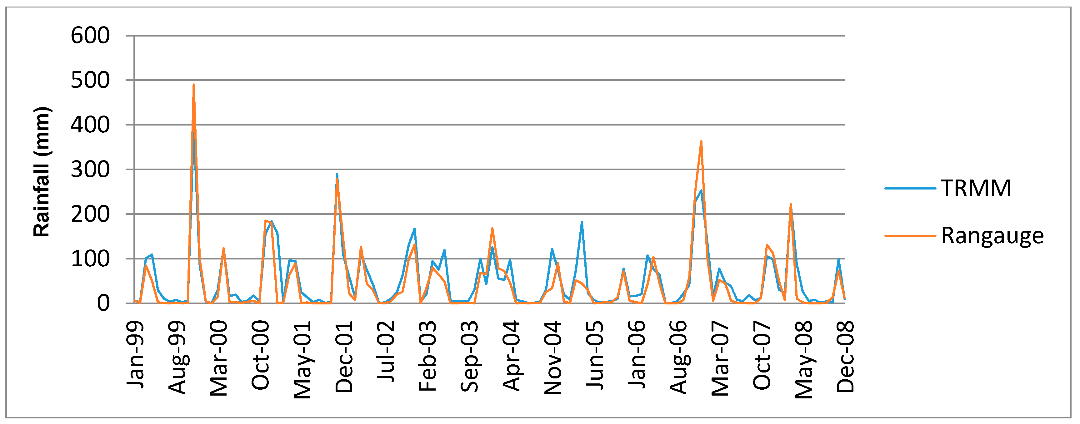
A comparison of rainfall data from the rain gauge and TRMM data was done using data for periods of the TRMM data 1998–2011 which were found not have gaps in the respective rain gauge datasets. Figure 2 shows time series plots comparison of the monthly values of the TRMM and rain gauge datasets for Kampi ya Mawe station.

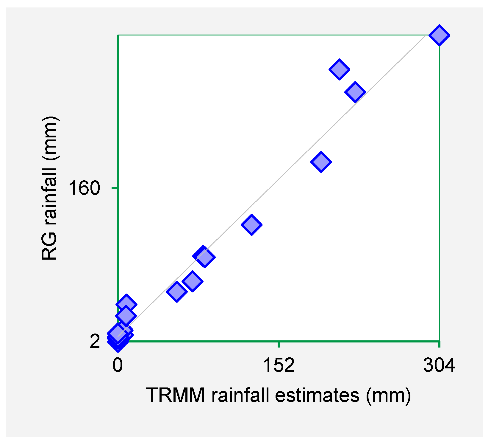
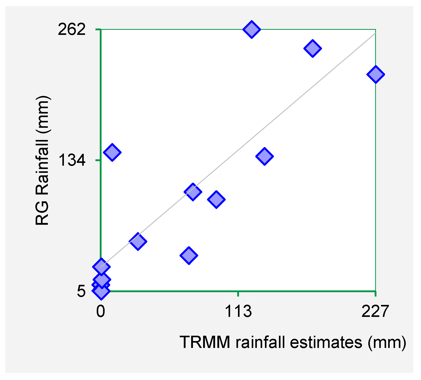
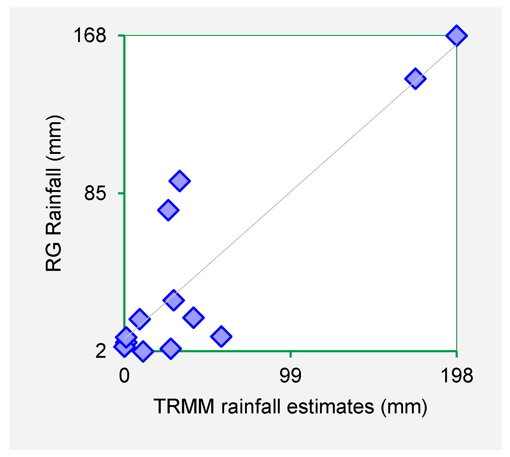
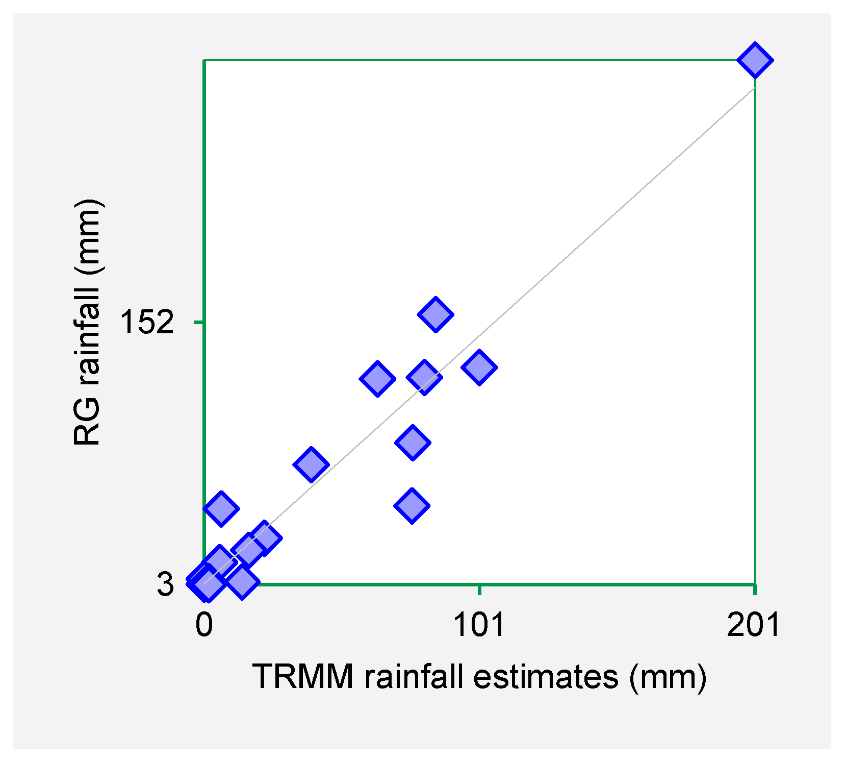
From Figure 2 it is observed that the TRMM datasets fit well with the rain gauge datasets for Kampi ya Mawe station. The close association of the rain gauge and TRMM datasets were further confirmed with the scatter plots of respective stations. Figure 3, Figure 4, Figure 5 and Figure 6 show the scatter plots for Mutonguini, Kambi ya Mawe, Kitui and Mutomo. The scatter plots were done for the month of rain gauge and TRMM data for selected years in the period 1998–2000.

The scatter plots indicate that strong positive association exist between the TRMM rainfall estimates and rain gauge-based rainfall observations. From the foregoing comparison of TRMM and rain gauge datasets, it is observed that TRMM rainfall datasets fit closely with rain gauge data series for Machakos, Makueni and Kitui County. As such it is inferred that TRMM rainfall estimates are a viable dataset for use in infilling missing rain gauge data gaps.

3.2. Infilling Missing Values of Rain Gauge Data

Missing data gaps in rain gauge datasets were infilled following the MOVE.2 approach. The MOVE.2 infilling model required stepwise approach to be able to account for special discontinuities. The rain gauge and TRMM datasets were arranged into annular sequences of monthly data series such that each month of the year had its own time series of rainfall data. Therefore, for each rain gauge and corresponding TRMM there was 12 series of annular sequence of month data time series (that is the sequence of all January data points for the period of interest for each respective station). In this arrangement for the station with the long missing data gaps (for example Mutonguini with 24 consecutive missing gaps), the missing gaps were reduced at most to two missing data gaps for infilling at the furthest point of estimation.

Following the MOVE.2 approach, stations whose missing gaps occurred earlier than January 2007, had only less than 10 data points of TRMM to be used in the regression. This was so because TRMM rainfall estimates commence in January 1998. As such, the infilling method discussed here applied only for missing gaps occurring at January 2008 onwards. Separate MOVE.2 regression relationships were developed for the stations Kambi ya Mawe, Mutonguni, Kitui, Mutomo, Kisasi, Lukenya, Matungulu, Matiliku and Mutito Forest.

For example, the estimated infilled value for Kitui station for the month of January 2009 followed the Equation (19).

$$\mathrm{Y}’\left(\mathrm{i}\right)={\mathrm{M}}^i\left(\mathrm{y}\right)\left(\mathrm{Jan}\right)+\frac{\mathrm{S}\prime \left(\mathrm{y}\right)\left(\mathrm{Jan}\right)}{Var\left(TRMM\right)\left(Jan\right)}\left[TRMM\left(Jan\right)-Mean for TRMM\left(Jan\right)\right]$$

(19)

This equation was used to estimate the value of infilled rain gauge missing gaps for January 2009 in Kitui station. The subsequent gaps occurring in the months of February 2009–December 2009, were filled by using the appropriate TRMM value for the respective months as in Equation (19).

Table 2. MOVE.2 parameters used in computation of infilled values for Kitui Station.

	Jan	Feb	Mar	Apr	May	Jun	Jul	Aug	Sep	Oct	Nov	Dec
m’(y)	56.51	62.86	137.91	158.59	67.92	9.98	3.435	6.84	11.531	58.28	274.44	108.90
S’(y)	1727.02	15776.68	1959.56	795.49	1174.06	12.37	7.166	23.74	206.21	6013.48	2924.27	18701.36
M(x)	75.53	26.35	107.83	152.71	69.06	8.93	7.11	12.60	12.03	32.302	187.36	88.02
M(y)	54.4	59.2	127.9	162.2	69.8	10.1	4.3	8.0	15.1	62.5	246.3	94.1
à	4.4	−8.8	−13.2	−8.8	−7.33333	−6.6	−6.16	−5.86667	−5.65714	−5.5	−5.37778	−5.28
y’(2007)	57.8	97.77	144.13	157.71	66.20	9.97	2.96	5.67	5.47	35.24	275.17	137.03
y’(2008)	55.2	27.96	131.70	159.48	69.65	10.01	3.91	8.02	17.61	81.33	273.72	80.77
X2	91.9	74.3	219.4	386.1	159.1	17.1	15.6	25.9	43.7	193.3	437.7	66.4
X1	2.8	9.2	52.8	215.5	113.3	10.8	15.3	20.6	38.7	143.5	239.4	29.5
M(X1)	51.47	8.55	89.36	165.27	66.47	8.32	3.85	10.97	10.57	32.67	209.65	111.17
M(X2)	56.82	20.88	183.22	116.06	46.70	4.91	9.78	13.30	12.02	30.69	201.02	72.30

and

Table 3. MOVE.2 parameters used in computation of infilled values for Mutonguini Station.

	Jan	Feb	Mar	Apr	May	Jun	Jul	Aug	Sep	Oct	Nov	Dec
m’(y)	71.61	27.15	115.70	155.69	72.205	9.34	6.61	9.25	11.74	31.88	200.2	93.56
S’(y)	6265.06	852.11	1579.48	574.96	3281.37	14.26	7.39	157.19	12.60	55.51	6776.38	17067.16
M(x)	68.05	20.18	89.82	169.99	63.73	7.28	5.51	10.98	11.31	52.86	235.46	91.14
M(y)	54.1	68.8	137.9	161.4	53.9	9.3	1.5	7.7	22.1	84.2	291.6	117.1
à	4.4	−8.8	−13.2	−8.8	−7.3	−6.6	−6.16	−5.8	−5.6	−5.5	−5.3	−5.2
y’(2007)	67.5	27.75	119.17	156.29	75.94	9.45	6.41	4.18	11.70	31.8	217.5	112.4
y’(2008)	75.69	26.55	112.22	155.09	68.46	9.23	6.81	22.69	11.80	31.91	183.06	74.71
X2	150.28	59.89	140.34	299.01	117.68	9.14	13.23	46.73	41.86	96.18	411.8	281.66
X1	131.82	14.67	30.55	124.005	44.36	6.57	10.65	32.39	15.50	44.51	71.41	38.31
M(X1)	37.21	6.40	82.83	187.81	58.85	6.45	3.72	9.38	10.01	40.45	227.02	133.44
M(X2)	50.11	7.60	140.87	157.18	45.79	5.10	6.63	11.05	11.44	65.8	263.05	55.06

show the MOVE.2 parameters used to compute the infilled values following equation 16 for Kitui and Mutonguini station (Kambi ya Mawe, Mutomo, Kisasi, Lukenya, Matungulu, Matiliku and Mutit forest). Similar parameters were computed to infill gaps in other stations. One hundred and forty-five data gaps for nine stations infilled in this method.

For the first month of long running data gap, the value of the coefficient à changes with the value of N1 and N2. This change affects the computed value of S’(y) which is estimated variance of the infilled series. The value of N1 changes due to overlap of the months for the preceding year. However, the equation of the infill remains the same for the subsequent year because of the effect of the change in N1 to N1 + 1 and N2 (1st gap for the year) form intrinsic part of S’(y).

The equation was developed with MOVE.2 approach with the intention to preserve mean and variance. Subsequent infilling of other data gaps followed the MOVE.2 process. The MOVE.2 equation was only applied at N1 and N1 + 1 depending on the number of data gaps for each month at each station. For each station, the regression equation was applied to estimate the respective value of the data gap. In this method, each month at which data was estimated was considered independent of the previous estimate.

Table 4. Distribution of number of data points infilled with MOVE.2 estimated values for respective stations.

Station	Jan	Feb	Mar	Apr	May	Jun	Jul	Aug	Sep	Oct	Nov	Dec
Mutomo							1	1	1	1	1
KYM	1	1	1	1	1	1	1	1	1	1	1	1
Mutonguni	2	2	2	2	2	2	2	2	2	2	2	2
Kitui	2	2	2	2	2	2	2	2	2	2	2	2
Kisasi	2	2	2	2	2	2	3	3	3	3	3	3
Lukenya	2	2	2	2	2	1	1	1	1	1	1	1
Matungulu	1	1	1	1	1	1	1	1	1	1	1	1
Matiliku	1	1	1	1	1	1	1
Mutito Forest	1	1	1	1	1	1	1	1	1	1	2	2

shows the number of data gaps infilled for the respective months for the stations.

3.3. Evaluation of Infilled Data Series

MOVE.2 values were evaluated for precision and accuracy in estimating the rain gauge values. The evaluation involved comparison sampled series of rain gauge data which were removed from the series and replaced with estimated values following a jacknife approach of replacement. Following the approach described in Section 2.3.3, MOVE.2 values were computed for gaps which were created by removing some rain gauge data. 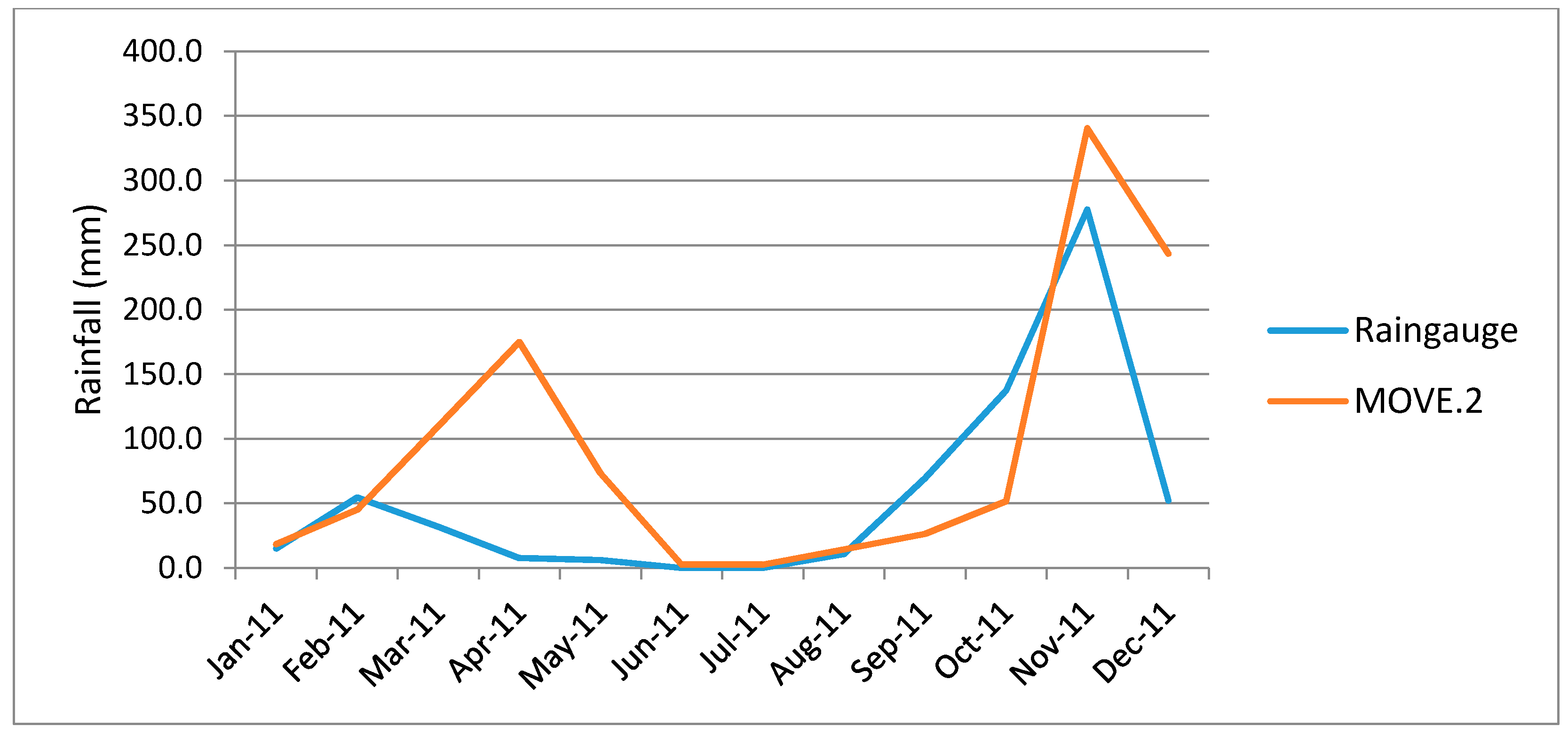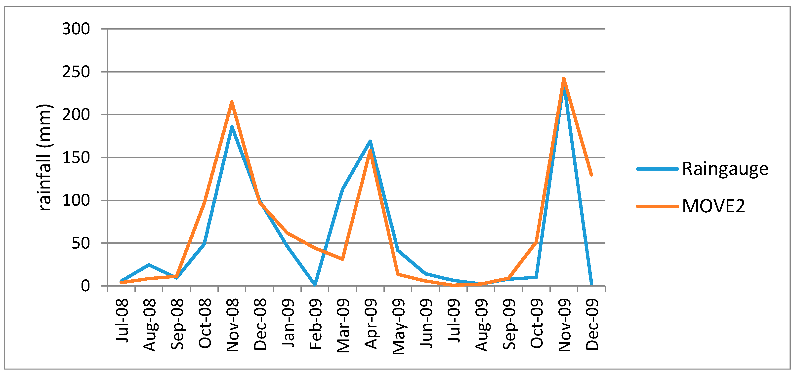Figure 7 and Figure 8, show plots of infilled data plotted against the rain gauge data in the removed areas for Kambi ya Mawe and Kisasi stations respectively. From the figures it is observed that the MOVE.2 infilled values follow the rain gauge data closely, but they are not a one-on-one match.

3.3.1. Comparison of Descriptive Statistics

Statistical parameters Mean, Median, standard deviation (Std. Dev), standard error of the mean (Std. Err. Mean), Minimum, Maximum, Skewness and Kurtosis were used to compare the MOVE.2 values infilled in the gaps where rain gauge data had been removed. In this analysis, the difference between the respective summary statistics of the rain gauge values and the MOVE.2 estimates were evaluated. Altman and Bland [38], recommended the use of the difference approach for comparison of summary statistics. The evaluation was done based on a non-parametric approach considering only the arithmetic difference of the statistics. For each station, the arithmetic difference in the summary statistics (Median, Standard Deviation, Standard Error of the Mean, Maximum and Minimum, Skewness and Kurtosis), of the samples originating from the samples of monthly values of rain gauge and MOVE.2 values were evaluated.

Table 5. Differences in Descriptive Statistics of rain gauge values and MOVE.2 estimates.

		Mean (mm)	Median (mm)	Std. Dev (mm)	Std. Err. Mean (mm)	Minimum (mm)	Maximum (mm)	Skewness	Kurtosis
Kambi ya Mawe	2007	8.965	9.191	−1.925	−0.556	2.763	10.115	−0.069	0.318
	2008	−19.541	19.85	−59.335	−17.129	−0.1	−173.3	−0.598	−0.924
	2009	16.085	29.75	−5.392	−1.557	9.363	0.7	−0.655	0.59
	2010	16.425	19.6	1.881	0.542	9.8	23.9	0.213	0.824
Lukenya	2007	12.858	10.1	10.953	3.162	5.1	43.5	0.262	0.94
	2008	0.091	12.15	−6.604	−1.906	3	4.9	0.398	0.626
	2010	12.641	17.65	7.717	2.228	4	43.5	0.286	0.398
Mutomo	2007	9.317	30.55	−36.1	−10.422	8.2	−121.5	−0.185	−0.02
	2008	6.992	1.95	0.084	0.025	2.1	5.7	−0.039	−0.061
	2009	8.3	15.3	9.366	2.703	2.1	44.2	0.334	0.995
	2011	9.691	8.55	9.596	2.77	2.1	28.8	−0.295	−0.881
Matiliku	2007	−2.533	6.15	−13.159	−3.798	5.4	−21.8	0.041	0.278
	2008	−0.925	−2.2	−3.101	−0.895	1.9	−16.7	−0.135	−0.834
	2010	−0.759	−0.6	2.681	0.774	−5	−10.3	−0.471	−0.801
	2011	52.5	−0.45	117.609	33.951	−1.4	408.8	0.15	0.756
Mutitu	2007	−3.85	14.95	−25.843	−7.46	3	−41.2	0.423	0.983
	2008	−1.942	10.5	−11.219	−3.238	3.5	−31.1	−0.092	−0.234
	2009	6.241	2.6	−6.774	−1.956	3.9	17.6	0.371	0.213
Matungulu	2007	7.458	34.15	−24.599	−7.101	−2.3	−125	−0.152	−0.372
	2008	10.425	33.25	−7.593	−2.192	−3.4	−15	−0.496	−0.386
	2009	−17.267	−36.85	−15.965	−4.609	5.8	−51	0.275	−0.414
	2010	12.584	34.67	−7.166	−2.069	8.6	13.3	0.335	0.288
Kisasi	2007	−11.579	6.2	−42.752	−12.342	7.1	−138.3	−0.473	−0.107
	2010	−42.725	−16.35	−84.65	−24.437	2.1	−273.3	−0.163	−0.026
Kitui	2007	−17.667	4.5	−32.676	−9.433	0.9	−90	0.02	0.507
	2008	−3.192	−1.85	−3.975	−1.147	4.3	−3.5	−0.078	−0.278
	2011	58.192	14.35	66.058	19.07	−1.8	129.3	−0.553	−3.166
Mutonguini	2007	−13.058	15.5	−31.919	−9.214	1.9	−31	0.805	4.868
	2008	−15.041	0.55	−18.554	−5.356	−1.7	−48.3	0.385	2.043
	2009	50.75	15.05	73.712	21.279	−0.6	189.7	−0.394	−2.096

shows the computed differences of the summary statistics.

Difference in the Standard Error of the Mean

The standard error of the mean (SE of the mean) estimates the variability between sample means that were obtained when multiple samples from the same population. In this study, the difference between the standard error of the mean of the samples of rain gauge values and standard error of the mean of the samples of the MOVE.2 estimates, were used to compare the difference in variability of the mean of the rain gauge values and the values of computed MOVE.2 estimates placed at gaps previously created by removing the rain-gauge values against the true rain-gauge values at those respective positions. Reading from Table 5, lower values (less than 2 standard deviations), of the difference of the standard error of the mean indicate closeness to precision of the MOVE.2 estimates to the rain gauge values.

In this way, the difference in the standard error of the mean as indicated in Table 4 is an indication of the deviation of the MOVE.2 estimates from the actual values of variability of the mean. The units of the standard error of the mean are rainfall units (millimetres—mm). The standard error of the mean is a good indicator of the precision of the estimated MOVE.2 values to infill respective rain-gauge values. This analysis is in line with inference made by Altman and Bland [38], that 95% of observations fall within 2 standard deviations. The difference in the standard error of the mean summary statistics viewed in this manner therefore indicates close proximity for all the samples of MOVE.2 values and rain gauge values analysed.

Thus, in this analysis the arithmetic difference between the standard error of the mean of the MOVE.2 infilled values and standard error of the mean of the rain gauge values indicates closeness of the estimated (MOVE.2 values) to the actual data (rain gauge values) for each of the removed data gaps.

Difference in the Median

The median is a measure of location which is useful, particularly when a distribution is skewed, and the end-values are not known, or when it is required that reduced importance be attached to outliers. This consideration is necessary for the purpose of measurement of errors. Given that the median is the 2nd quartile, 5th decile, and 50th percentile, the median values in this study were used alongside the minimum and maximum values of rain gauge data to determine the central location of the data series and compared the same with that of the MOVE.2 infilled series.

From Table 5, it is observed that the difference in the skewness and kurtosis of the two samples data sets is small (less than 1). The low difference analysed imply that the skewness and kurtosis of the samples of the rain gauge data series and the MOVE.2 values are in close proximity. This is an indication that the infilled datasets do not significantly affect the skewness nor the kurtosis of the data series. This is inferred due to the fact that the distribution of the differences in skewness and kurtosis was always symmetrical about zero, and of magnitude less than one, in the respective periods for all the stations.

It is also worth noting that the differences analysed in the minimum values was always low (less than 10 mm of rainfall). The minimum rainfall occurs during the non-seasonal months of January, February, June, July, August and September. On the other hand, systematic errors for TRMM estimates have been observed to be more during the non-rain months, since aggregation of hourly TRMM always gives values more than zero [39]. The difference in the maximum value is affected by large outliers associated with the influence of rainfall by topography. TRMM measurements have also been associated with low skill on highly variable topographic regions [39]. Reading from Table 5, the infilled data series was observed to maintain the location of the median value as exhibited by the rain gauge series without affecting the skewness nor the kurtosis of the distribution of the infilled series for all the stations.

The Wilcoxon signed test is a non-parametric statistical hypothesis test used when comparing two related samples, matched samples, or repeated measurements on a single sample to assess whether their population mean ranks differ (i.e., it is a paired difference test). Given that the median is a measure of the central location in a data series. The Wixcon test was used to evaluate the closeness of the median to the position of the mean.

The requirements for the Wilcoxon Signed-Rank Tests for Paired Samples where z_i = y_i – x_i for all i = 1, …, n, are as follows:

The z_i are independent;

x_i are differences data;

The distribution of the z_i is symmetric (or at least not very skewed).

The null hypothesis was thus stated as follows:

H₀: the distribution of difference between paired values of the median of the samples of rain gauge data and the corresponding MOVE.2 values is symmetric about zero. (That is, any differences are due to chance). The test was done at values of α = 0.05 and n = 14 (i.e., the number of values of the TRMM period of rainfall data). From the statistical table we find that Tcrit = 21 (two-tail test). Since T_critical = 21 < 35.5 = T. The decision to reject or accept the null hypothesis was done at α = 0.05 (i.e., p ≥ 0.05).

Table 6. Results of Wixcon Test Comparing the Difference between the mean of the Median of the samples of MOVE.2 Estimates and the Rain gauge Values.

Month of the Year	KYM	Mutomo	Lukenya	Matiliku	Mutito	Matungulu	Kisasi	Kitui	Mutonguini
Jan	1	0	1	1	1	0	0	0	0
Feb	0	0	0	0	0	0	0	0	0
March	0	1	0	1	0	0	1	0	0
April	1	1	1	1	1	1	1	1	1
May	0	0	0	1	0	1	1	0	0
June	0	0	0	0	0	0	0	0	0
July	0	0	0	0	0	0	0	0	0
August	0	0	0	0	0	0	0	0	0
September	0	0	0	0	1	1	0	0	0
October	1	1	1	1	1	1	1	1	1
November	1	1	1	1	1	1	1	1	1
December	0	1	1	1	1	1	1	1	0

below shows the decision (1) to accept and (0) to reject the null hypothesis, of the Wixcon test and so conclude there is no significant difference between the two data series.

From Table 6, it is observed that a mix of both acceptance and rejection of the null hypothesis is analysed for the different samples at different stations. Notable in this analysis is the scenario in the months of April, October, November and December where all the stations accepted the null hypothesis indicating therefore that the median was close to the mean in these months. The months of February, June, July, August and September exhibited rejection of the null hypothesis, thus indicating that the median location was not close to the mean. It is worth noting that the months of April, October, November and December are the months with the highest seasonal rainfall exhibiting the high rainfall amounts in the study area. Mahmud et al., [40], analysed similar characteristics between TRMM estimates and rainfall in Peninsular Malaysia and noted that correlation between TRMM and monthly rainfall was good during the wettest months in all local climate regions. Thus, borrowing from Mahmud et al., [40] it may be inferred that the difference indicated in the median probably originate from the TRMM data rather than induced from the MOVE.2 analysis approach.

3.3.2. Parametric Evaluation of Infilled Data Series

An error of measurement is the difference between an obtained value and its theoretical true score counterpart. Two types of errors were used to evaluate the accuracy and precision of the estimated MOVE.2 data series, including Mean Absolute Percent Error (MAPE), and analysis of regression residuals.

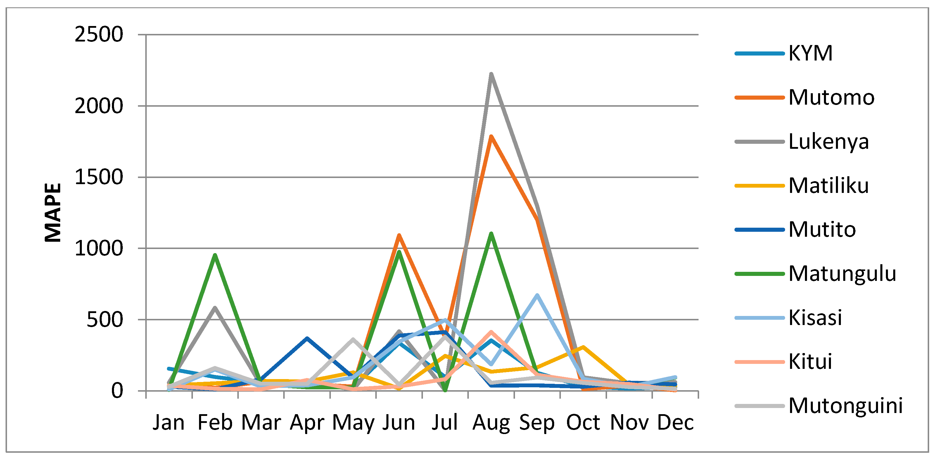
Mean Absolute Percent Error (MAPE)

MAPE was used as a measure of accuracy of the infilled data series of the sampled MOVE.2 data to estimate the respective rain gauge rainfall values, Hyndman and Koehler [41]; Wilson [42] recommended that MAPE be used for evaluation of cross-sectional estimates such as the MOVE.2 estimates of rain gauge rainfall. MAPE expresses the accuracy of the MOVE.2 infilled data series as a percentage of the rain gauge data series. Figure 9, shows the distribution of MAPE for the nine stations in the study.

From Figure 9, it is observed that low values (less than 100%), of MAPE are analysed for the months of January, March, April, May, October, November and December. These months are the period of seasonal rainfall for the study area. However, a drastic increase and extremely high values of MAPE are analysed for the months of February, June, July, August and September, which also happen to be months of low rainfall amounts.

Given that the MAPE is a relative measure which expresses errors as a percentage of the actual data, it provides in this analysis an easy and intuitive indication of the distribution of errors in the infilled series of estimated rain gauge values. It also gives a way of judging the extent, or importance of errors, such that in this case an error of 10% when the actual value is 100 (making a 10% error) is more worrying than an error of 10 when the actual value is 500 (making a 2% error). This aspect is clearly indicated with the low values of error for the months of high seasonal rainfall and the high values of error during the months of low seasonal rainfall. Thus, the distribution of the MAPE indicated in Figure 9 is an indication of relatively acceptable distribution of errors for the infilled MOVE.2 derived estimates.

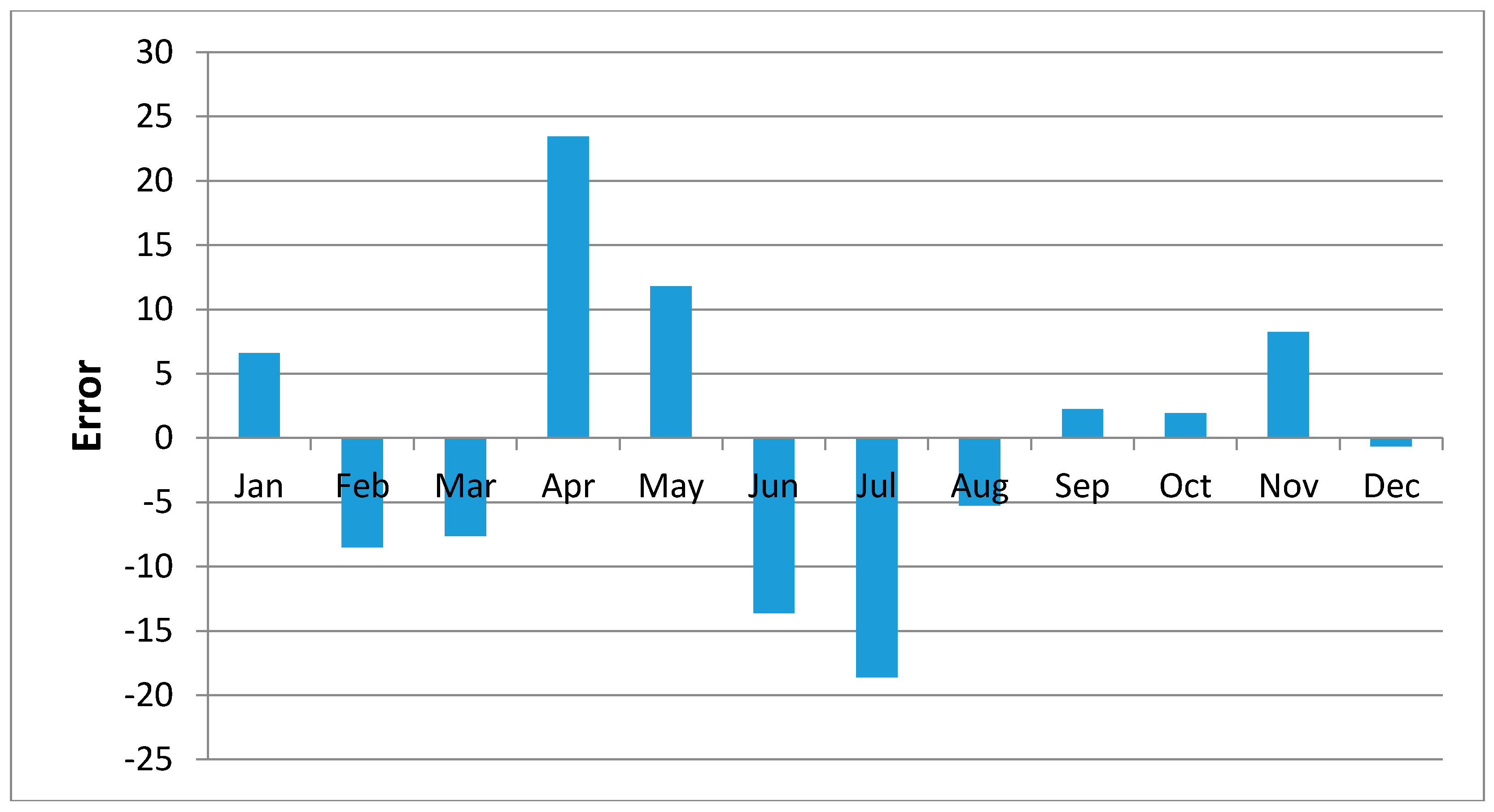
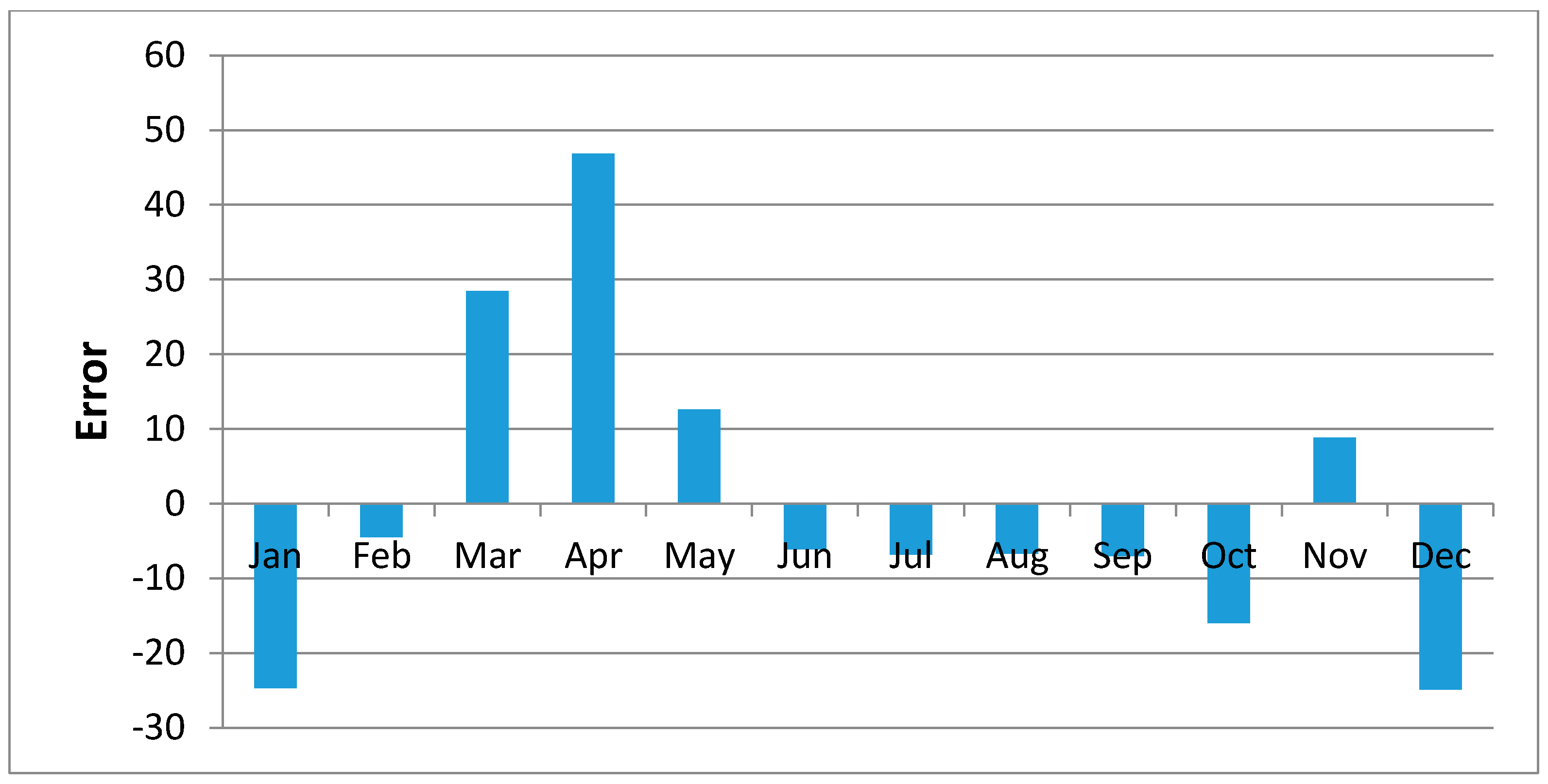
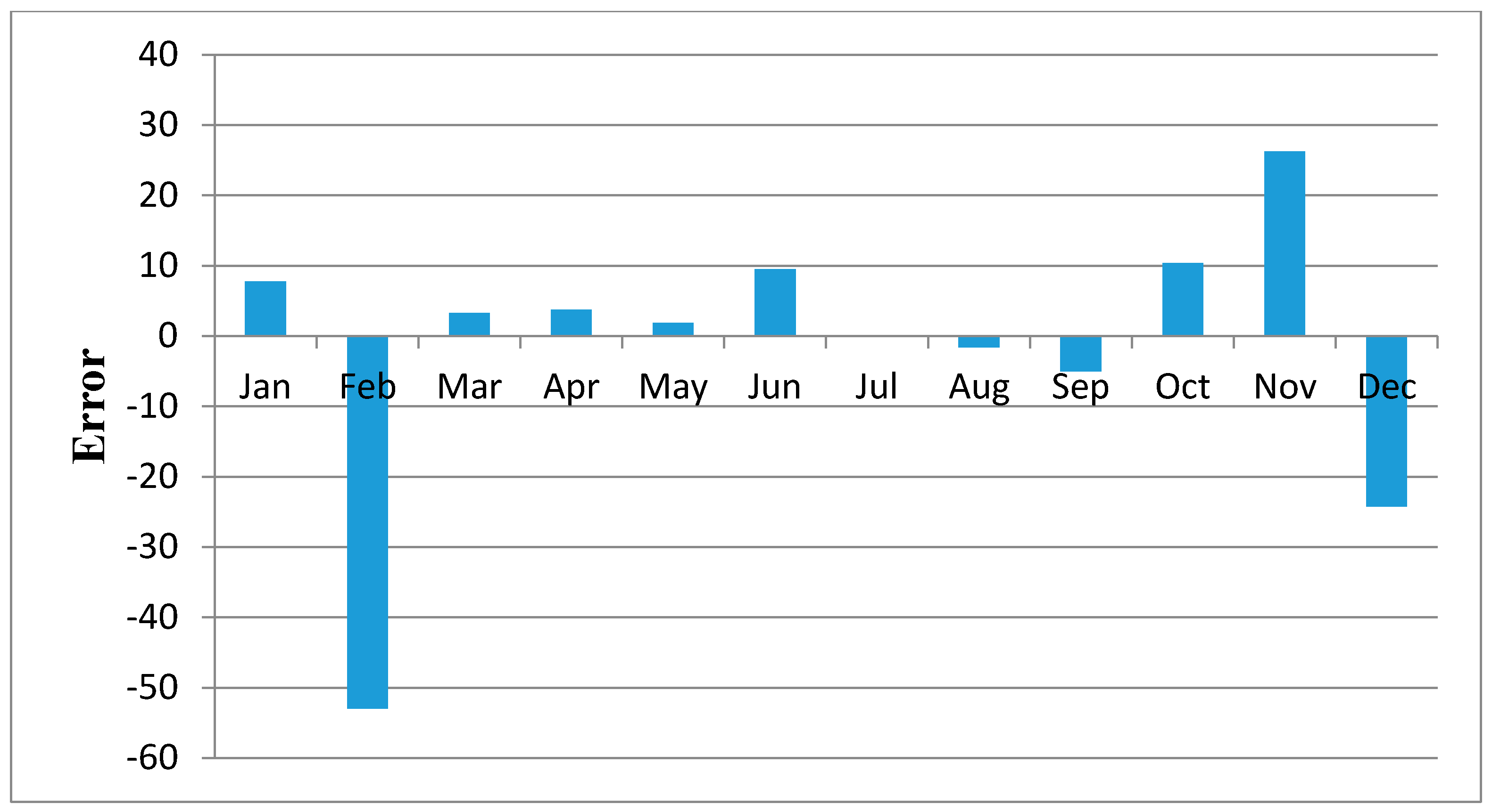
Error in the Regression Analysis

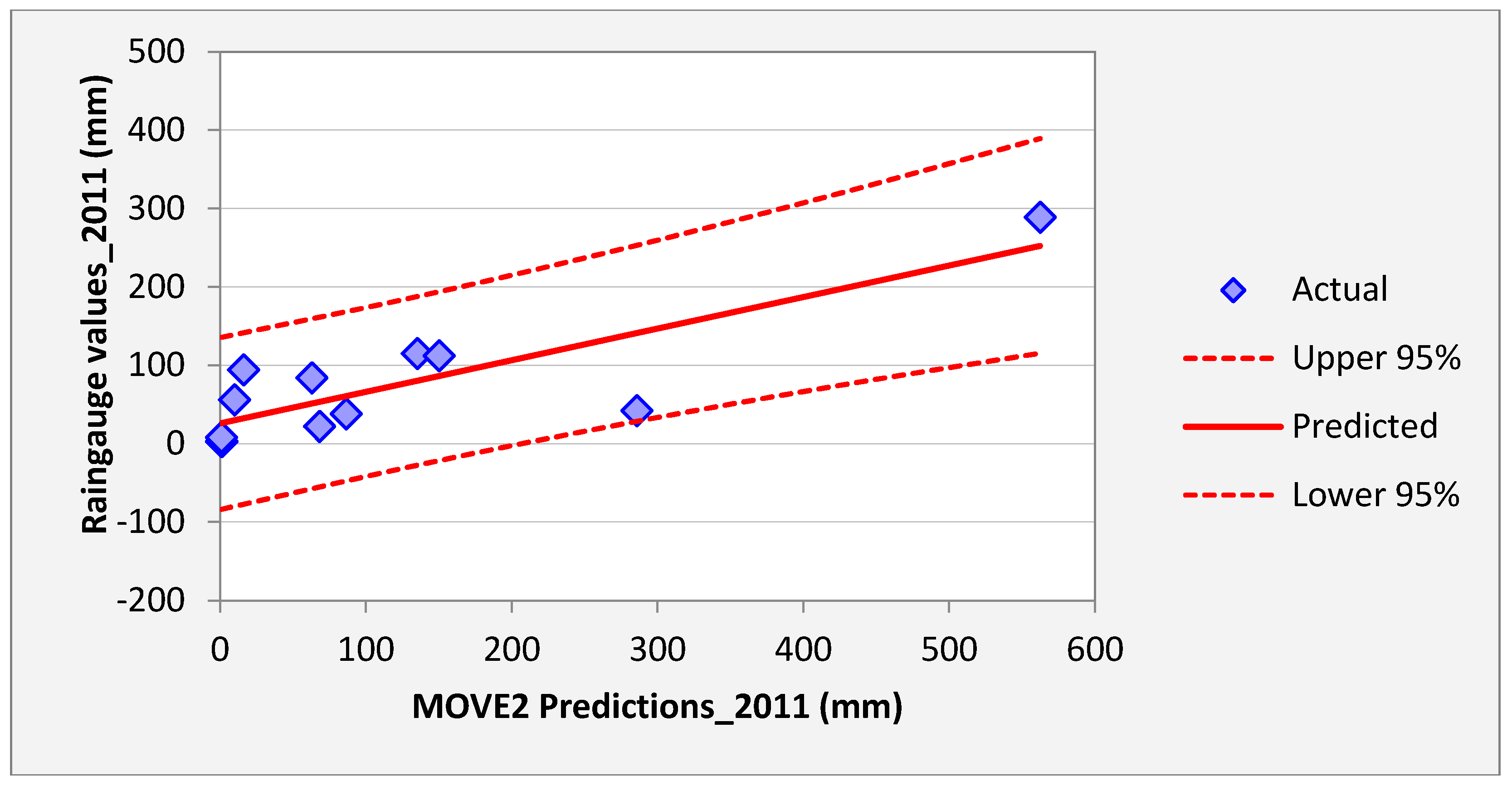
Figure 10 shows regression results of the samples of Kisasi station for the year 2011. The plot shows the MOVE.2 values for the year 2011 against rain gauge values for the same year for the station. In this plot each point plotted on the figure indicates where the MOVE.2 values are plotted on the x-axis, and the accuracy of the observations are on the y-axis. The distance from the solid line (perfect agreement) indicates the magnitude of the error (residual) on the prediction of the value. Values above the solid line mean the prediction was too low, and values below the solid line mean the prediction was too high. In this regression analysis, it is observed that the computed MOVE.2 values are close to the rain gauge values with relative small margins of errors. This analysis was repeated for all the stations and similar results were observed.

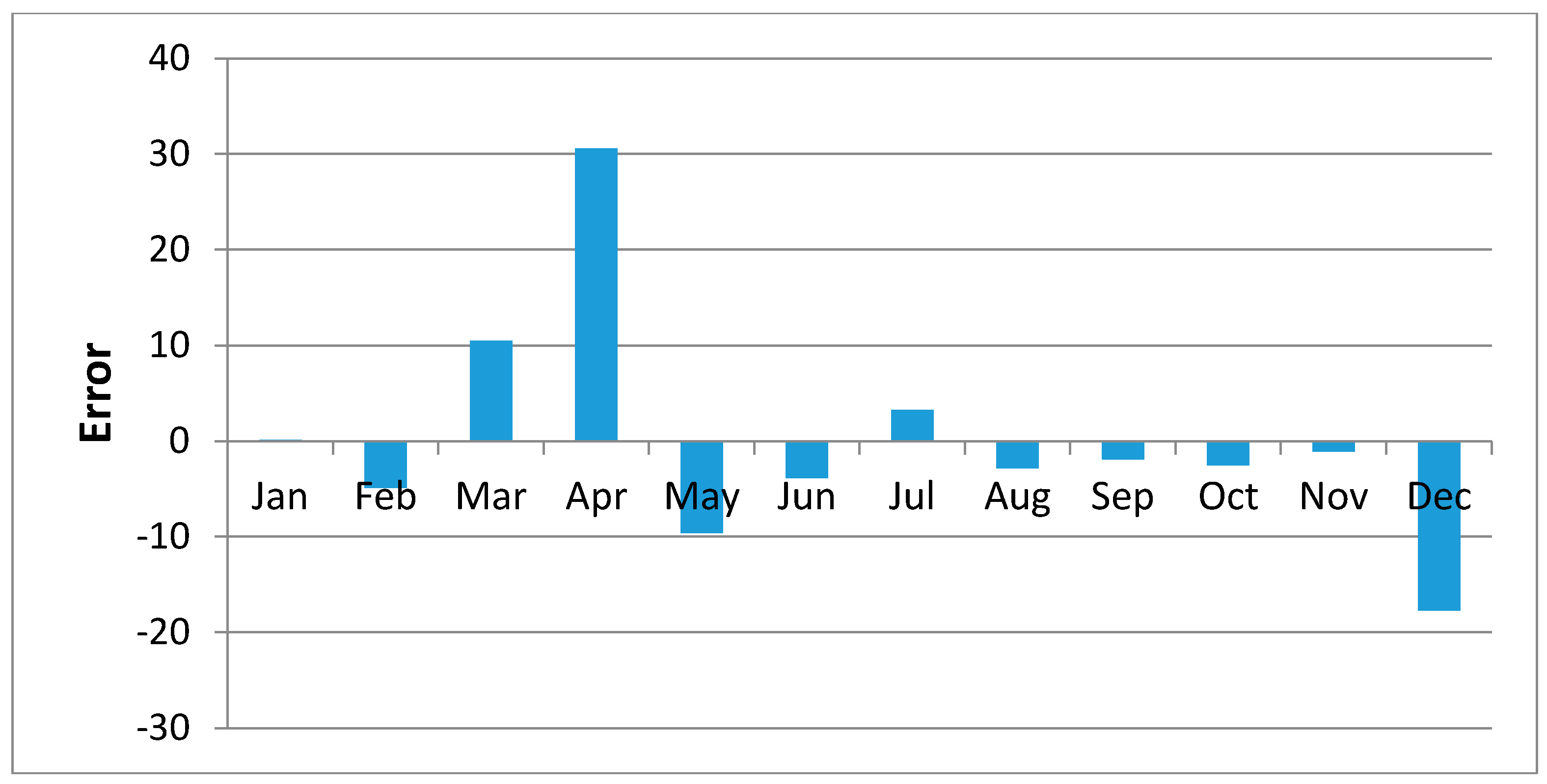
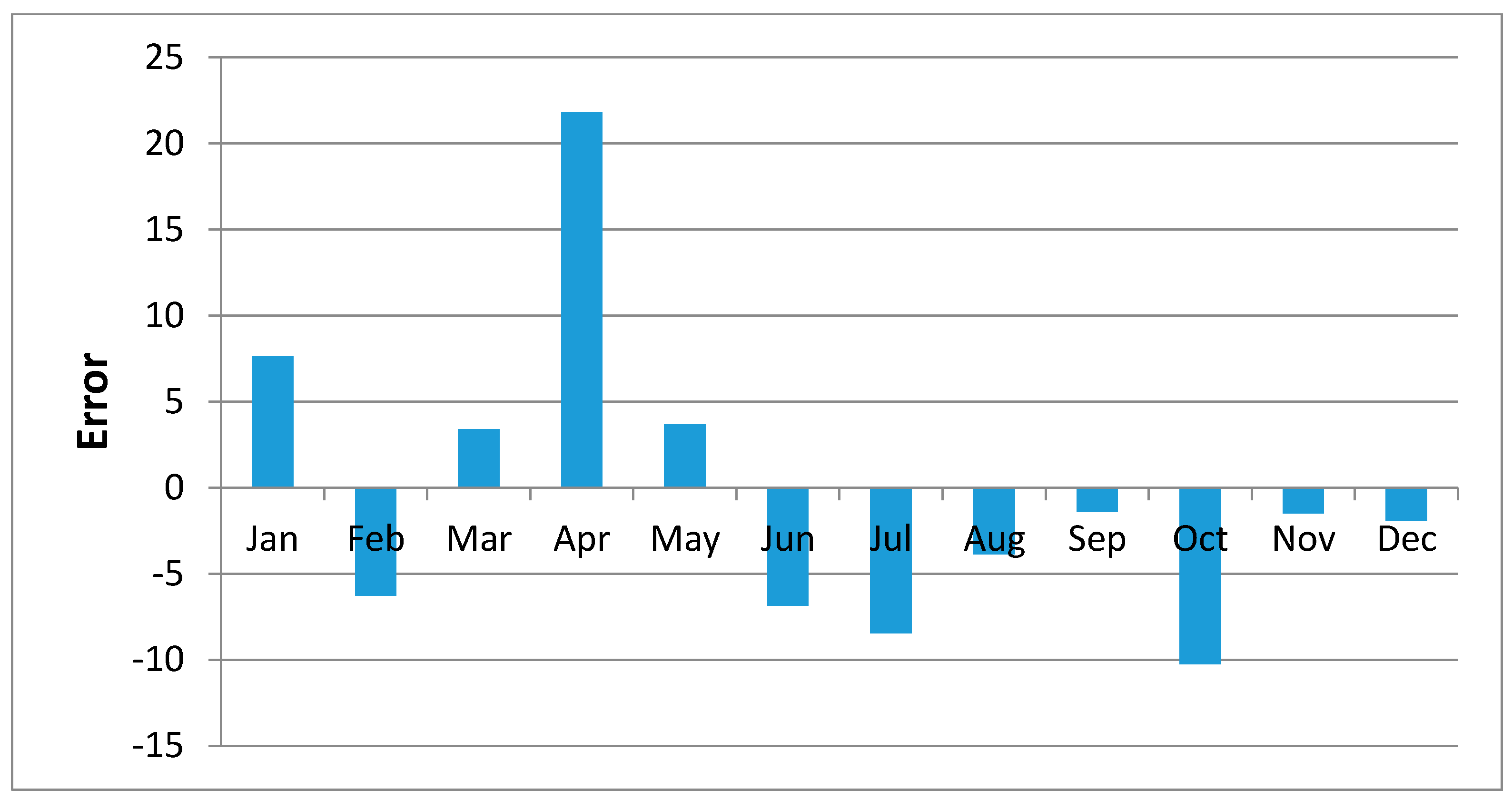
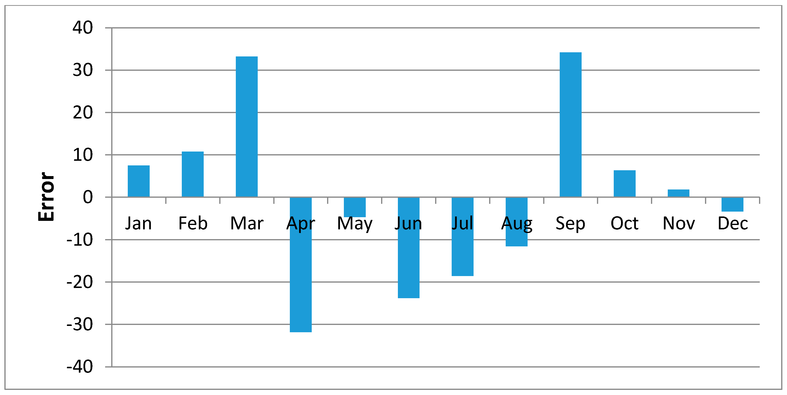
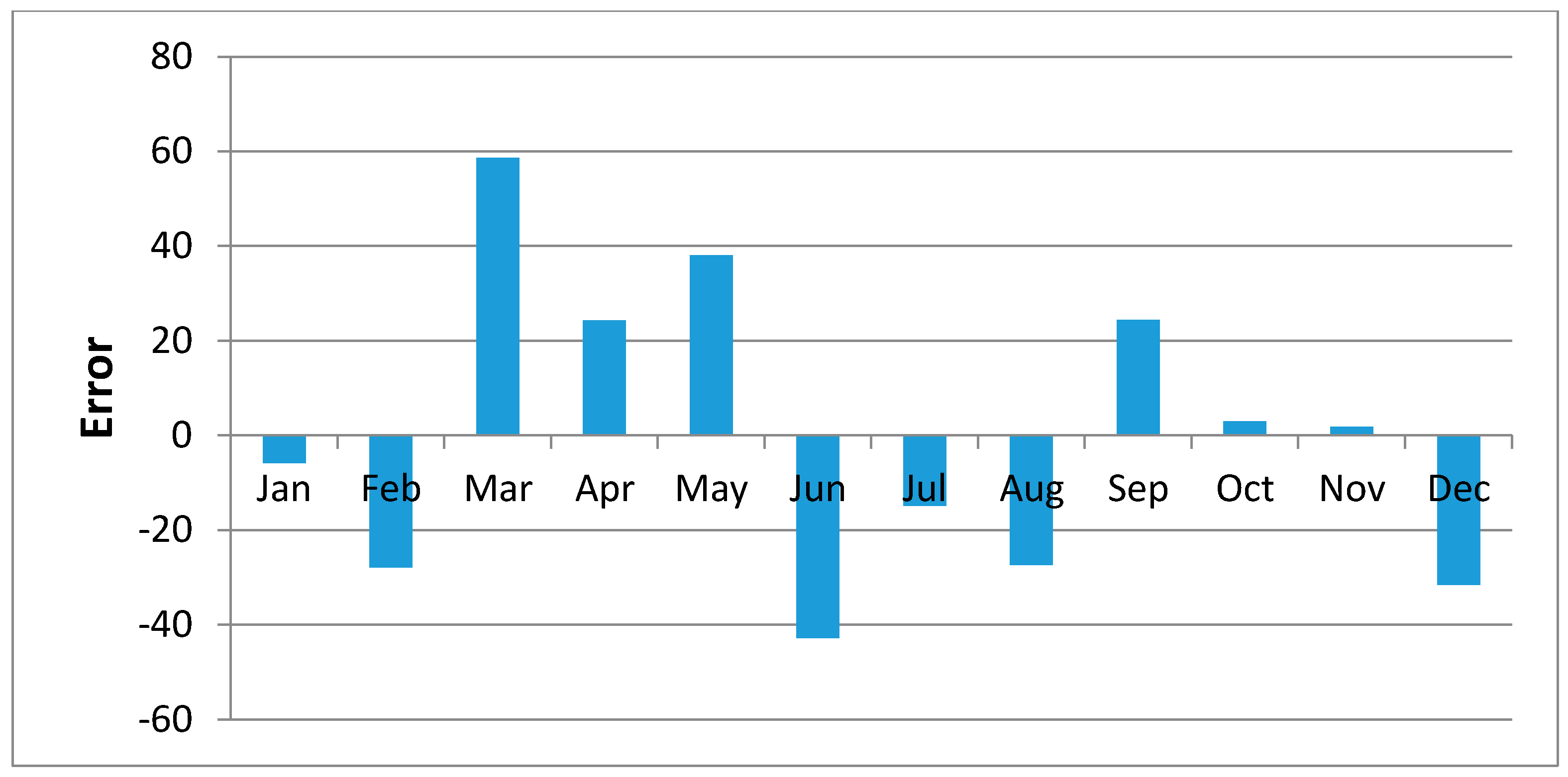
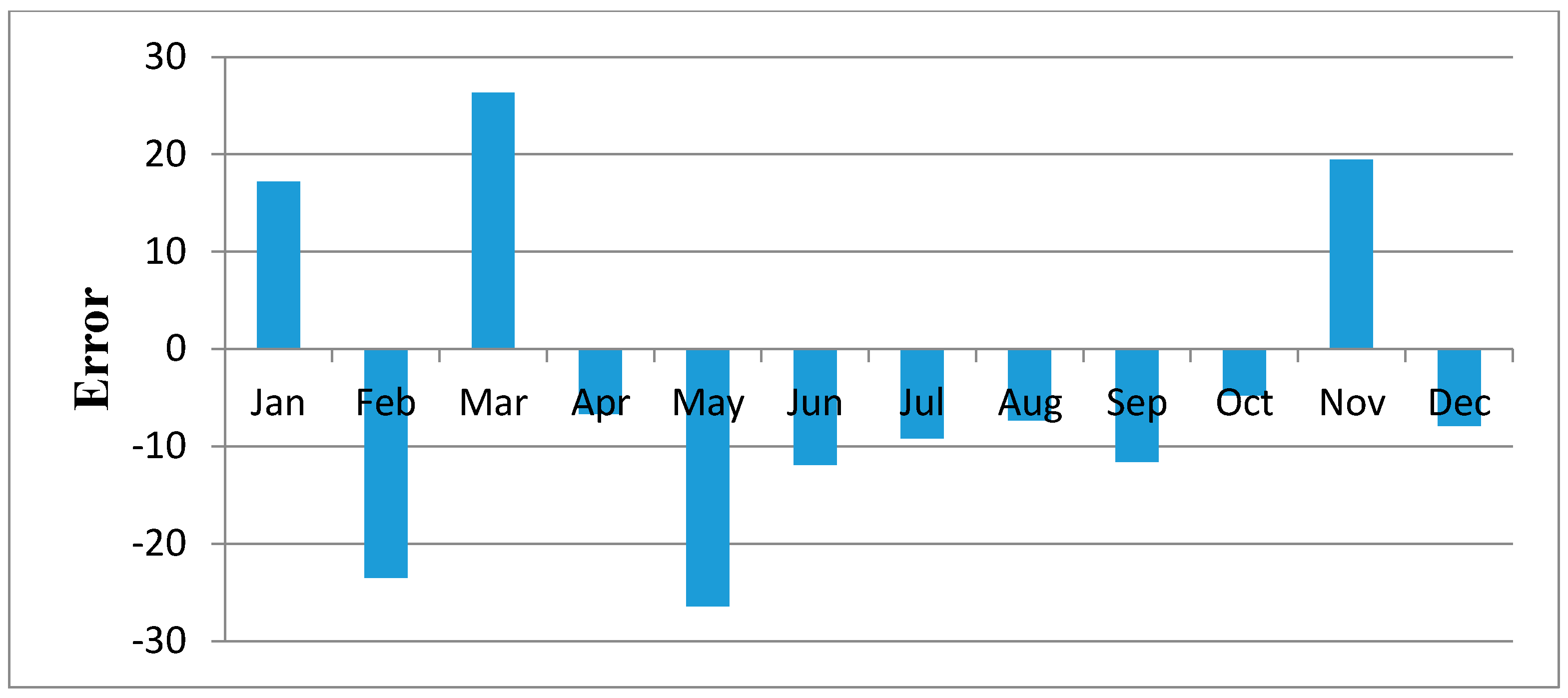
Figure 11, Figure 12, Figure 13, Figure 14, Figure 15, Figure 16, Figure 17, Figure 18 and Figure 19 shows plots of the mean of regression residuals for each station. The mean of regression residuals was computed for the number of years which were sampled for each of the stations. From the plots of mean regression residuals, it is observed that the mean residuals are not evenly distributed vertically, such that there are positive and negative residuals. It is also observed that the residual exhibit high variability but certain patterns are easily discerned from the plots. For example, it is notable that the during the months of October, November and December which also are the main rainfall season of the study area, the residuals exhibit low values (less than 30 mm) for all the stations. The months of March and April exhibit high variability of the regression residuals across the stations. This is despite the two months being months of seasonal rainfall in the study area. The high variability of regression residuals during the March–April–May season may be related to the high unreliability of rainfall during the period [43]. Glover et al., [44], estimated the unreliability of rainfall in the April to May season in the South Eastern parts of Kenya within which this study was conducted at 40%. The 40% unreliability of seasonal rainfall depicts a situation of erratic characteristics of rainfall with high variability.

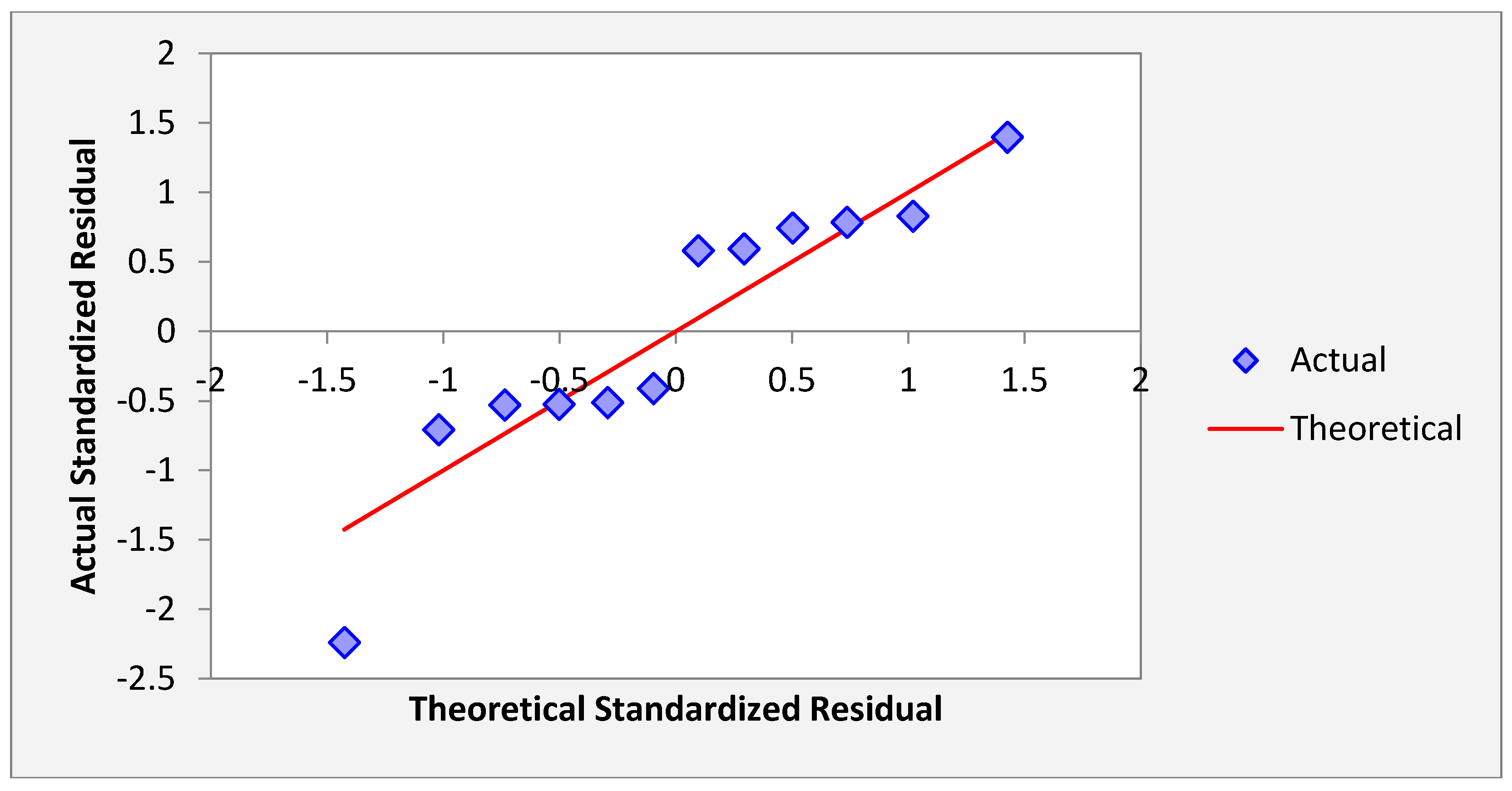
Figure 20 shows the normal probability plot of the residuals. In Figure 20, the pattern of the residuals curve is approximately linear indicate that the residuals are normally distributed hold.

3.4. Test of Equality of the Mean and Variance

The statistical tests t-test and F-test were based on two approaches, first the data of the series generated with the jacknife sampling was arranged in the order of running calendar months (a series for each station for the sample period) containing data of the generated MOVE.2 values, and the dataset of respective rain gauge values arranged in a similar manner and the mean/variance of the two series were compared for equality in a t-test and F-test respectively.

The data of the series generated with the jacknife sampling was arranged along the annular month (a series of data of the order of annular modes representing year to year variability), month-month values beginning 1998 up to and including the year of which there was replacement with the MOVE.2 value). The sequence of the annular series was such as that the sequence of values was, for example: Jan 1998, Jan 1999, Jan 2000, ..., Jan 2011). A similar sequence for each of the 12 calendar months were developed. Two annular months series, one with the surrogate data and the other of rain gauge data within the sections without gaps were developed. The mean and variance of the two series were compared for equality in a t-test and F-test respectively. This approach applied only for the years preceding the gaps in the respective stations. The years within the gaps area as indicated in Table 1 and the years after the appearance of gaps were not included in the analysis.

3.4.1. Two-Sample t-Test for Equal Means

The two-sample t-test [45] was used to determine if the means of the rain gauge data series and the MOVE.2 estimated series are equal. The test, was used to determine whether a significant difference exists or does not exist between two data sets. The t-test was also used to determine whether the two sample means of two independent samples come from the same population. In the t-test, the formula for calculating “t” is given in equation [46].

The null and alternative hypotheses were stated as follows:

H₀: µ₁ = µ₂; the means are equal

H₁: µ₁ ≠ µ₂; the means are different

This is a two tailed test because the Null Hypothesis does not specify a direction, only the condition of equality.

The t-test indicates that there is not enough evidence to reject the null hypothesis that the two means are equal at the 0.05 significance level. The t-test therefore concluded that the two datasets rain gauge datasets and MOVE.2 infilled datasets have the same means at the 0.05 significance level and that the two datasets may be considered to come from the same population.

3.4.2. F-Test for Equality of Two Variances

An F-test is a statistical test in which the test statistic has an F-distribution under the null hypothesis. An F-test [47] was used to test if the variances of two populations are equal. The F-test used is a two-tailed test. The null hypothesis was stated as:

H₀: σ₁ = σ₂

H₁: σ₁ ≠ σ₂

The F Statistic was computed as:

F = s₁/s₂

where s₁ and s₂ are the sample variances. The more this ratio deviates from 1, the stronger the evidence for unequal population variances. The variances are significantly different if F is greater than the appropriate value in the F table. The degrees of freedom for the numerator are (n₁ − 1), where n₁ is the sample size for the group with higher variance. Degrees of freedom for the denominator are (n₂ − 1), where n₂ is the sample size for the denominator group. This is a two-tailed test.

The F-test indicated mixed analysis with many favouring acceptance of the null hypothesis and two stations favouring rejection of the null hypothesis. The stations of Kisasi, Kitui, Mutonguini, Mutitu, and Lukenya the null hypothesis was accepted for all the samples. The station of Kisasi indicated rejection of the null hypotheses for two samples 2007–2008 and 2011 while Matiliku indicated rejection of the null hypotheses for one sample 2010–2011 The F test indicates that there is enough evidence to reject the null hypothesis that the two variances are not equal at the 0.05 significance level.

Notable in this analysis is that those months which had incidents favouring the acceptance of the null hypothesis were mainly the months of high rainfall including high seasonal rainfall such including March, April, May, October, November and December indicating that the variance of the two samples MOVE.2 generated surrogates and the rain gauge dataset are equal. The months of low rainfall including January, February, June, July, August and September indicated rejection of the null hypothesis indicating that the variance of the two samples MOVE.2 generated surrogates and the rain gauge dataset are not equal. Details of the computation of the t-test and the F-test may be found in the Appendix of this paper.

3.5. Confirmation of Preservation of Mean and Variance

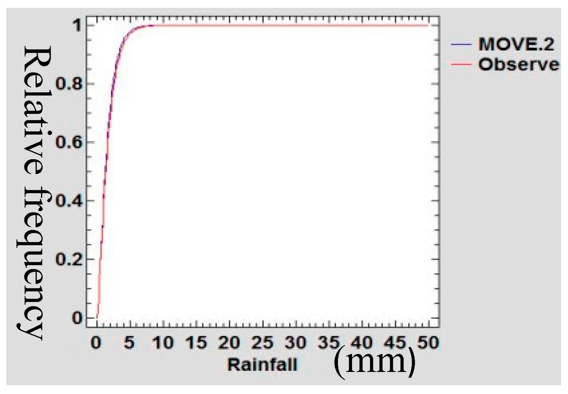
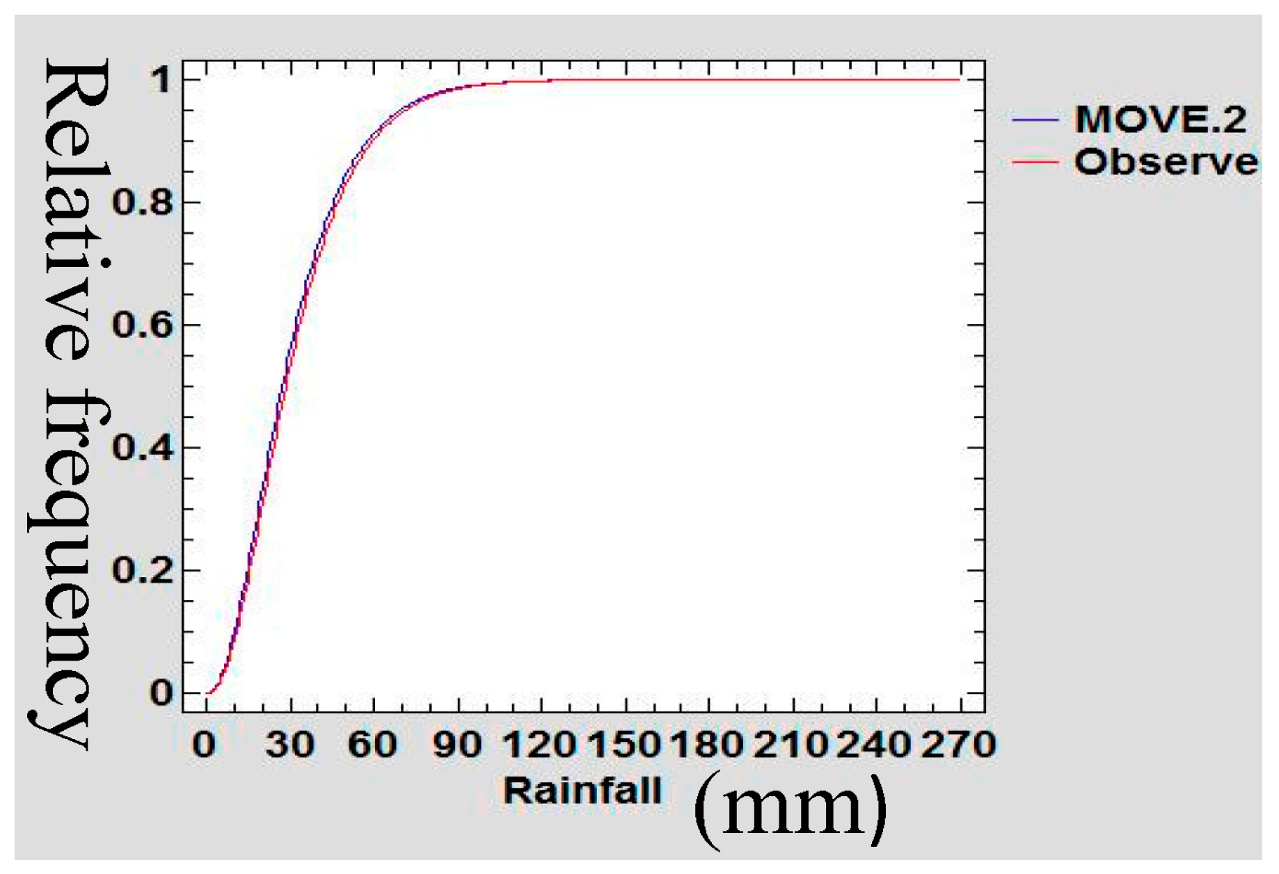
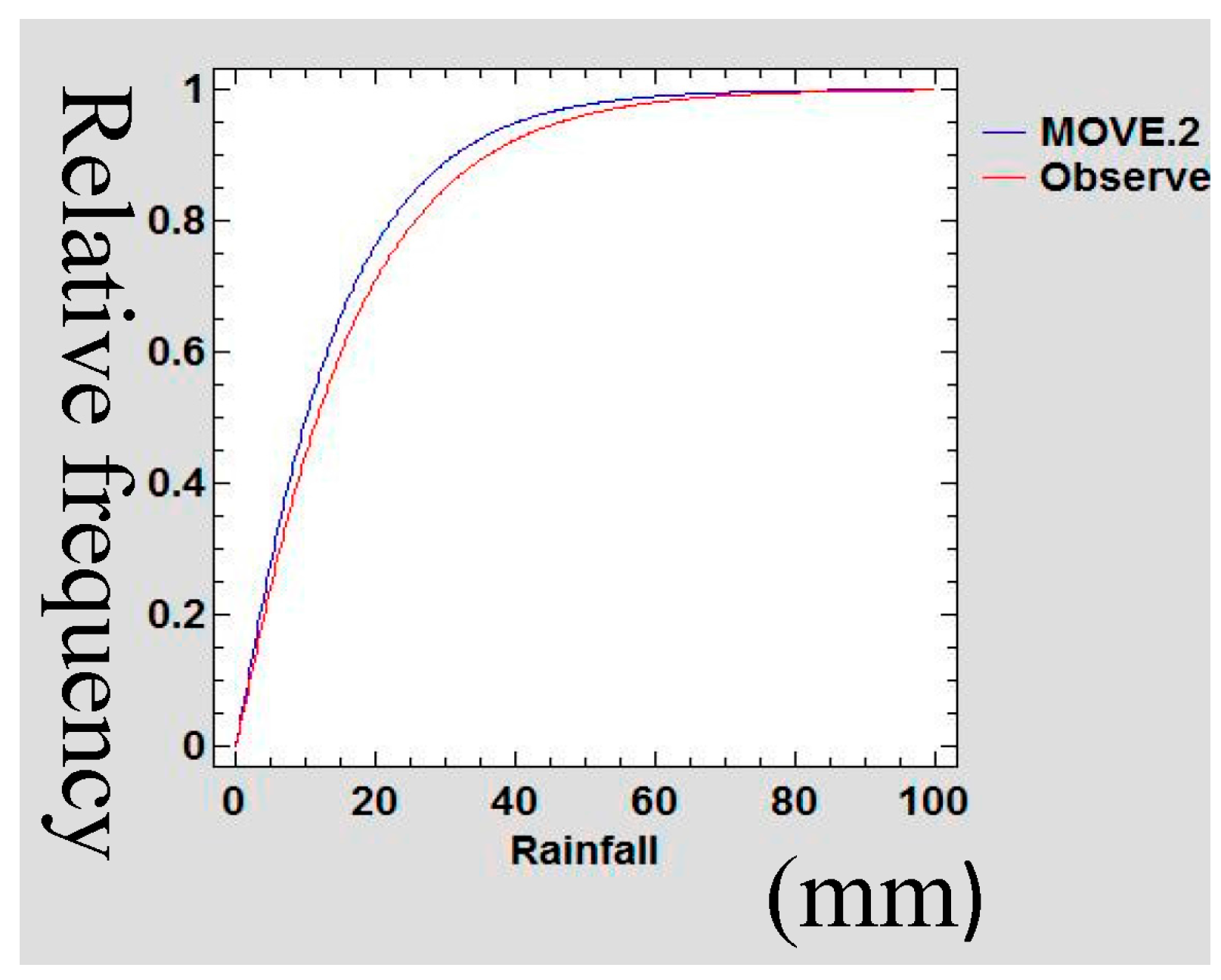
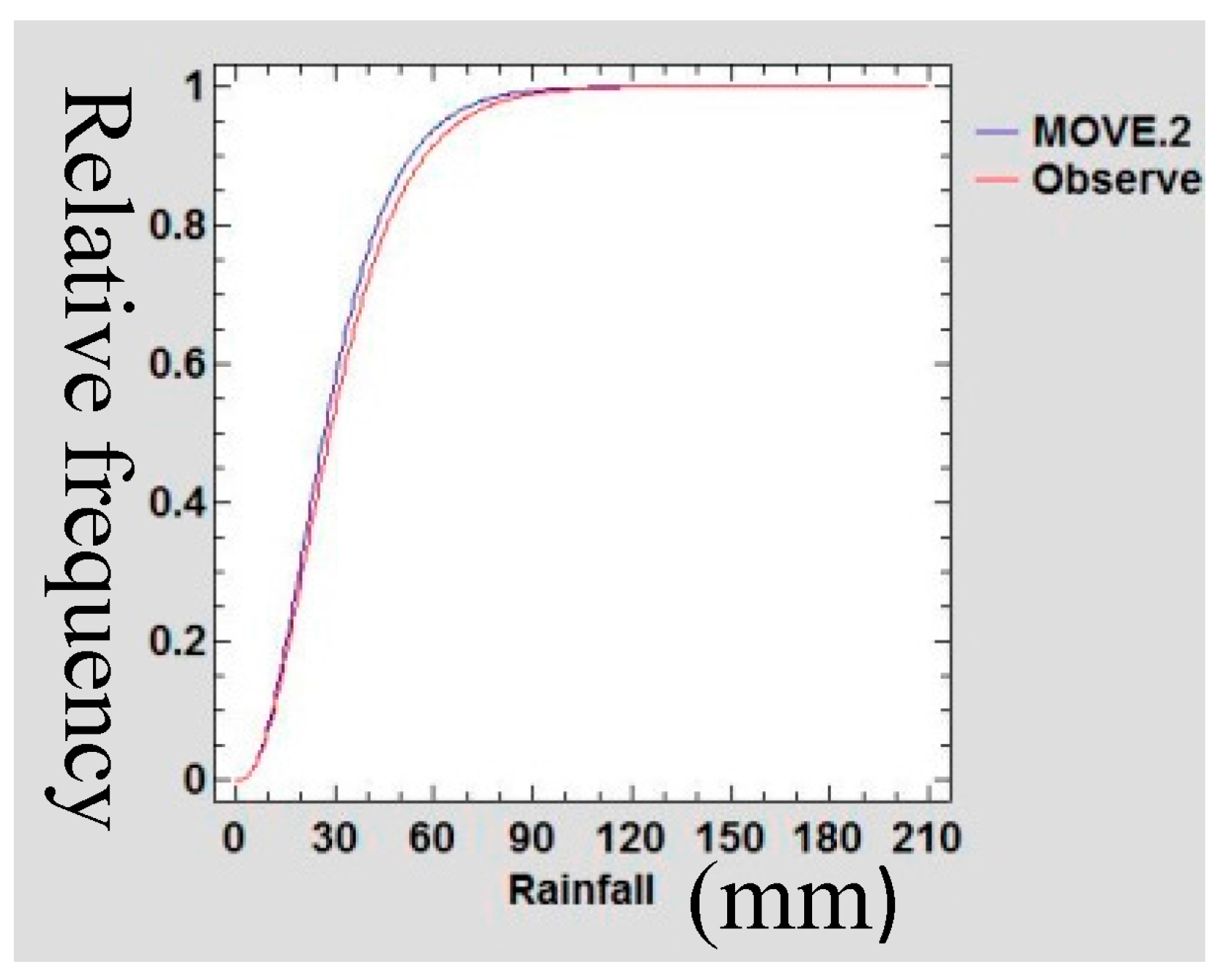
A Gamma probability density function (PDF) was used to confirm the preservation of mean and variance of the infilled data series of rain gauge data following Theiler et al., [48]. The data sets of the extended MOVE.2 were fitted into a gamma distribution function and statistical tests of equality of mean and variance was done. Figure 21, Figure 22, Figure 23 and Figure 24 show the Gamma cumulative distribution function for Mutomo station comparing the plots of original data and that of the infilled data for the month of January. It is observed that the cumulative function of the extended dataset fit well with the distribution of the original data. Given that the gamma function fits well, it is an indication that the plots have similar parameters α and β for the two plots further confirming the assumption of preservation of mean and variance of the MOVE.2 approach.

3.6. Autocorrelation Test

Given that the infilled values were translated from different datasets, it is prudent to test for autocorrelation among the adjacent variables. If they are correlated, then this implies that the least-squares regression underestimated the standard error of the coefficients and predictors can seem to be significant when they may not [49]. The Durbin-Watson statistic was used to test for autocorrelation within adjacent values in the new series after infilling of the data.

Table 7. Durbin-Watson Statistic Matching the size of infilled datasets and Highest Number of Points infilled per month (n).

	Size of Infilled Dataset	Value of n	Upper Bound Value	Lower Bound Value	Durbin-Watson Statistic
Kambi ya Mawe	12	1	2	1	2.1
Mutonguni	24	2	2	1	2.32
Kitui	24	2	2	1	2.49
Mutomo	12	1	2	1	2.89
Kisasi	30	4	2	1	2.32
Lukenya	29	4	2	1	2.89
Matungulu	29	4	2	1	2.22
Matiliku	19	2	2	1	2.38
Mutito Forest	26	3	2	1	2.15

shows the values of Durbin-Watson statistic computed for each data series.

For autocorrelation test the critical limits are 2 − DL and 2 − DU. The hypotheses were stated as follows:

H₀: ρ = 0 (no serial correlation);

H₁: ρ < 0 (negative serial correlation)

If d < 2 − DU do not reject H₀, if d > 2 − DL reject H₀.

Since all the values of Durbin-Watson statistic are greater than 2, H₀ is not rejected and the conclusion is that there is no serial correlation in the infilled data series. The analysis of lack of serial correlation in the infilled data series serves to confirm the stationarity assumption of the extended series.

3.7. Goodness of Fit

Table 8. Correlation coefficient and the coefficient of determination for the years 2007–2011 for the respective stations.

	2007		2008		2009		2010		2011
	Corr. Coef.	R2	Corr. Coef.	R2	Corr. Coef.	R2	Corr. Coef.	R2	Corr. Coef.	R2
KYM	0.92	085	0.57	0.6	0.52	0.65	0.89	0.79	-	-
Matiliku	0.96	092	0.99	0.99	-	-	0.98	0.96	0.55	0.52
Lukenya	0.42	018	0.807	0.65	0.69	0.48	-	-	-	-
Mutomo	0.88	0.77	0728	0.89	-	0.86	-	-	0.92	0.85
Kisasi	0.94	088	-	-	-	-	-	-	0.83	0.69
Mutitu	0.94	0.87	0.95	0.91	0.84	0.71	-	-	-	-
Matungulu	0.60	0.36	0.90	0.81	0.69	0.65	0.94	0.82	-	-
Kitui	0.90	0.80	0.94	0.89	-	-	-	-	0.63	0.59
Mutonguini	0.98	0.96	0.97	0.95	0.84	0.71	-	-	-	-

shows the computed values of correlation coefficient and the coefficient of determination for the years 2007–2011 for the respective stations. Medium and high values of correlation coefficient and the coefficient of determination were analysed between the original rain gauge data series and the MOVE.2 surrogate series for the different years at all the stations.

3.8. Discussion

The intent of infilling missing data is to produce a time series which is relatively long that possesses statistical characteristics believed to be like those of the actual record for the station [50]. The reason for producing such a record is for use in simulation and optimizations related to potential water management decisions. This study demonstrated the extension of rain gauge records donated from TRMM rainfall estimates following a least square regression MOVE.2 approach. In this methodology, the study transferred the characteristics of distribution shape, serial correlation, and seasonality from the TRMM dataset to the rain gauge station record [51]. The analytical derivations, based on linear regression alone cannot be expected to provide records with the appropriate variability [52], and TRMM data series cannot be expected to provide records with the appropriate distribution shape or serial correlation as the rain gauge data series. This is so because the TRMM data series and rain gauge data series have substantial differences in terms of distribution shapes, serial correlation, or seasonality.

3.8.1. Viability of Infilled Data Series

The jacknife sampling approach used in this study for evaluating the infilled series involved removing one value from the annual month series of rain gauge data to enable estimation of the same following the MOVE.2 approach. The remove-1 jacknife, approach, however is known to give inconsistent variance estimators for non-smooth estimators such as the sample quantiles including the median [53]. This deficiency was overcome in this study by increasing the number of values removed, following a smoothness measure of the point estimator as recommended by Shao and Wu, [53]. In the analysis, there were 12 values removed on the running series of monthly rain gauge data sets in one jacknife sample of one annual month. Thus, it followed that for each annual month removed, there were a total of 12 running month series of values removed thereby achieving the required values for smoothness of estimator. The sampling methodology used in this study also follows very closely with the suggestions of Guo Hua et al., [54].

In estimating the median using a jacknife sampling approach, Guo Hua et al., [54] observed a lack of smoothness which seemingly was caused by the jacknife inconsistent estimate of the standard error. In this concern, Guo Hua et al., [54], suggested that instead of removing one value at a time in the jacknife, a number of values, equivalent to (d), be removed where n = r.d for some integer r. Guo Hua et al., [54], actually suggested removing out more than d = $\sqrt{n}$ when estimating the median, but fewer than n values to achieve consistency for jacknife estimate of standard error. These suggestions made by Guo Hua et al., [54], are similar to recommendation of Shao and Wu [53]. Therefore, since in the jacknife approach (used as explained in Section 2.3.3), considered the requirement for consistency as suggested by Guo Hua et al., [54] and Shao and Wu, [53], it is expected that the MOVE.2 values as evaluated in this study give a true picture of the capability of estimation of the rain gauge values.

The use of the MOVE.2 method produced infilled series with statistical characteristics (mean, variance and extreme values) of the rain gauge series. The MOVE.2 methodology has desirable properties that enable appropriate preservation of the parameters. The MOVE.2 methods also considered the two distributions as separate and distinct distributions with different parameters yet combining into one distribution with the same parameters. A probability density function (PDF) approach was used to confirm the preservation of mean and variance of the infilled data series of rain gauge data following Theiler et al., [48]. Sen and Eljadid, [55] indicated that the gamma distribution has appropriate probability distribution for describing monthly rainfall for arid and semi regions. The month data series of the infilled data sets were fitted into a gamma distribution function and statistical tests of preservation of mean and variance was done. It was observed that the cumulative function of the extended dataset fit well with the distribution of the original data. Given that the gamma function fits well, this is an indication that the plots have similar parameters α and β, confirming the assumption of preservation of mean and variance of the MOVE.2 approach.

No physical quantity can be measured with perfect certainty; there are always errors in any measurement. This means that the measurement of MOVE.2 estimates of rain gauge rainfall values, on a repeated basis as more gaps are infilled, certainly will contain errors [56]. The error analysis is an attempt to quantify the uncertainty resulting from the infilled values. The understanding of the errors also contributes to emphasizing the need for care in the measurement and application of refinement of the method for the purpose of reducing the errors. We can thereby gain greater confidence that the computed MOVE.2 values closely approximate the true value [57]. Error analysis in this study therefore expresses the uncertainties inherent in the estimated values of rainfall computed by the MOVE.2 approach for infilling in the rain gauge data gaps. As such it is inferred that the results of the error analysis are an indicator of the high quality of the extended data series. It is thus inferred that MOVE.2 approach enables maintenance of high quality rainfall data series even after the infilling of the extended datasets.

A mean-preserving spread is a change from one probability distribution (donor series) to another probability distribution (recipient series), which is formed by spreading out one or more portions of the donor probability density function while leaving the mean of the recipient series unchanged [58]. As such, in this study, TRMM data series have proven to be good at preserving the mean and variance contraction of rain gauge data series following Gentzkow and Kamenica [58].

A statistical test confirmed the significance of the similarity of the statistical parameters’ mean and variance of the infilled dataset for all the stations. In this study, therefore, it is inferred that the use of TRMM data series to infill rain gauge data following the MOVE.2 approach is the mean and variance preservation method. The approach agrees with Khalema [59], who showed that one can mix a baseline distribution with a Gamma distribution and obtain a mixture distribution which has mean and variance preservation capability.

3.8.2. Reliability and Validity of Infilled Data Series

Harvey et al., [50] identified three factors likely to influence reliability of data infilling, the nature of the donor station (TRMM in this case), the location of the station and duration of the gap and the infilling procedure. In this study, TRMM rainfall estimates were confirmed as a good fit of the rain gauge data. The MOVE.2 regression relationships were developed for rain gauge series and TRMM series data for each month of the 12 calendar months. In this approach the number of missing data gaps was reduced to a maximum of two data points for each month for the longest running series of missing data (24 months). Other stations had at most only one missing data point for the respective month. Giustarini [60] observed that best performances for infilling missing data was obtained when the gaps were comparatively short. In this study, the MOVE.2 approach used along the sequential annual months series reduced the long-running missing gaps to short gaps for the respective months series. As such, this study recommends the use of MOVE.2 in a sequential annual months approach for infilling rainfall data from TRMM estimates for effectiveness. It is also observed that the reduced number of missing gaps for infilling reduces the regression errors, thereby enhancing the reliability of results. This method also agrees with Henn et al., [61] that shorter missing gaps are easy to fill for all methods. Generally, in ordinary regression methods of data infilling, it follows that the RMSE increases with an increase in the proportion of missing values (gap size). Furthermore, the MOVE.2 approach demonstrated in this analysis, suggests reducing the gap size, thereby reducing the RMSE. Thus, the MOVE.2 approach, utilizing sequential annual months, enables the infilling to attain high accuracy even with long gaps of missing data.

4. Summary

This study tested a methodology for infilling missing gaps in rain gauge observed data series following the least squares regression. The study presented a methodology for infilling the rain gauge data series from a satellite based rainfall estimates. The satellite estimates were extracted from grid points nearest to the respective station. These satellite estimates were used as donor stations.

The study tested the use of the MOVE.2 approach using TRMM satellite data as a donor station. The study therefore addressed an imperative challenge for hydro-meteorological science, of long consecutive missing data gaps among the rain gauge observed data series. This is particularly true for the ASAL of Kenya and Africa whose data gaps are rampant in the hydro-meteorological data series, and also other parts of the tropics where TRMM data observations are available.

In the MOVE.2 approach, the coefficient of linear regression was interpreted as being of marginal effect. This marginal effect corresponds to how the dependent variable (rain gauge data) changes when the independent variable (TRMM data) changes by an additional unit holding all other variables in the equation constant. Based on the data used in this regression, adding one additional month of rain gauge record, corresponded to an increase in monthly rainfall. The sequential annual month arrangement of rain gauge rainfall records helped to operationalise the capability of MOVE.2 approach. With this approach the methodology enabled the preservation of the mean, variance and extreme value statistic for the infilled data series. As such the infilled rain gauge series maintained the same distribution as the observed series. It is, however, worth mentioning that the preservation of the variance was not always upheld, particularly for months of low seasonal rainfall. This observation was also noted for the median.

5. Conclusions

The results reported in this study provide researchers with a methodological framework that can be readily applied for infilling missing values of rainfall in rain gauge data series using TRMM satellite estimates as donor station. The approach has demonstrated capability of extending monthly rainfall values which remain similar to those observed by way of preserving the statistical parameters such as mean, variance and extreme statistics. The infilled values of rainfall have characteristics like those of the actual records they are intended to represent.

The methodology therefore serves a need as expressed by researchers, for development of generic data infilling methodologies which ensure consistency, auditability and effectiveness in the infilled series.

Infilling of missing rainfall data in the data series using the least square regression in MOVE.2 approach as used in this study promises robustness of methodology even in situations of large and extensive data gaps with a high proportion of missing values. The approach proposes a way of shortening long and running missing gaps into very short and manageable missing gaps. The infilling of short missing gaps as proposed here, promises quality of infilled data and hence quality of predictions for models which utilise the infilled data series. The method offers a viable alternative to traditional infilling approaches.

The results suggest that MOVE.2 utilizing TRMM data is effective for infilling rainfall data series in Machakos, Makueni and Kitui counties of Kenya. The TRMM rainfall products coupled with MOVE.2 approaches could therefore be considered as viable alternative data source for large-scale distributed rainfall analysis for development of hydro-meteorological models such drought early warning, monitoring and forecasting. The approach ensures a consistent and auditable approach towards infilling, which could find application in the ASAL of Kenya and for the tropical regions in general.