Highlighting the Role of Groundwater in Lake– Aquifer Interaction to Reduce Vulnerability and Enhance Resilience to Climate Change

Abstract
:1. Introduction
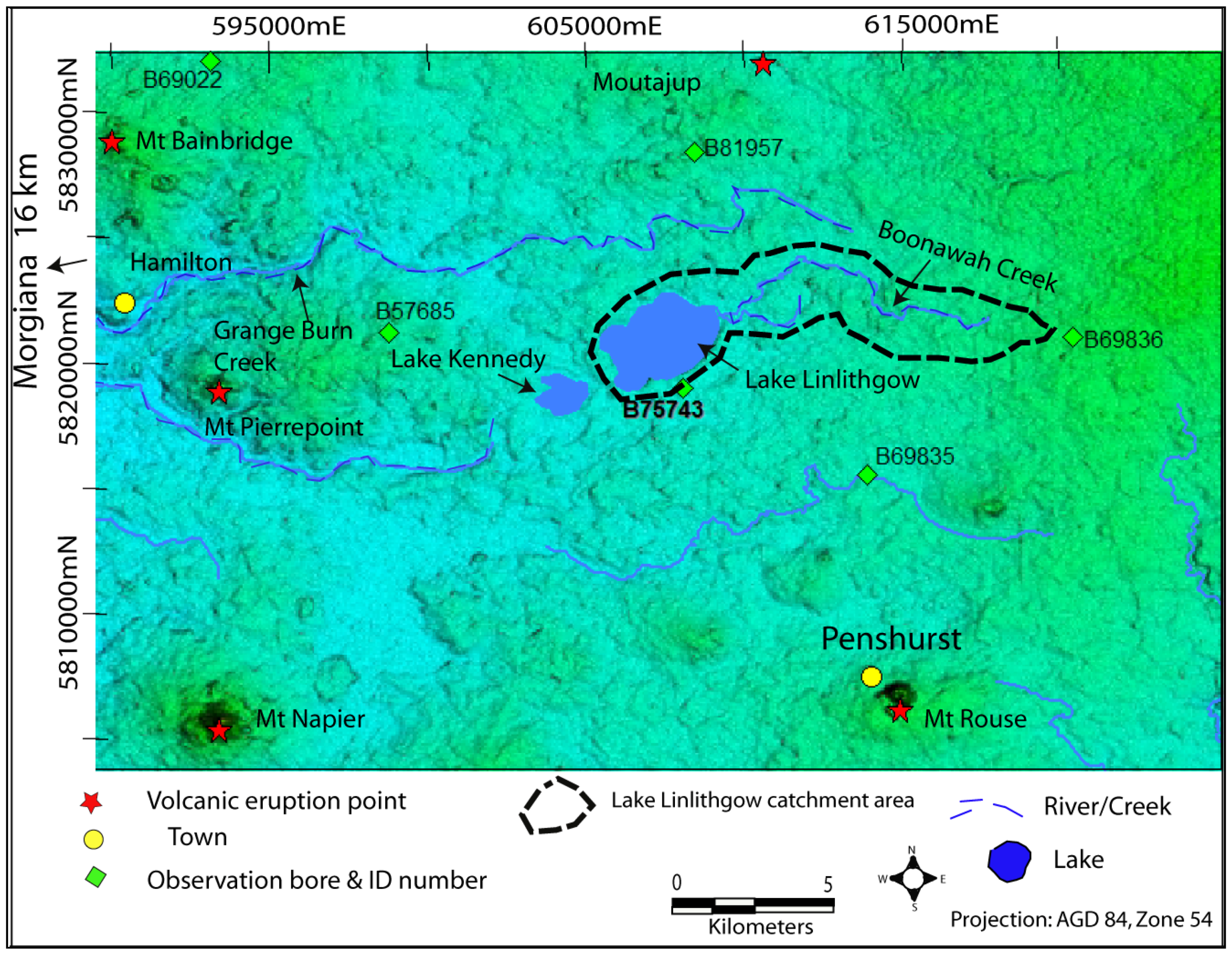
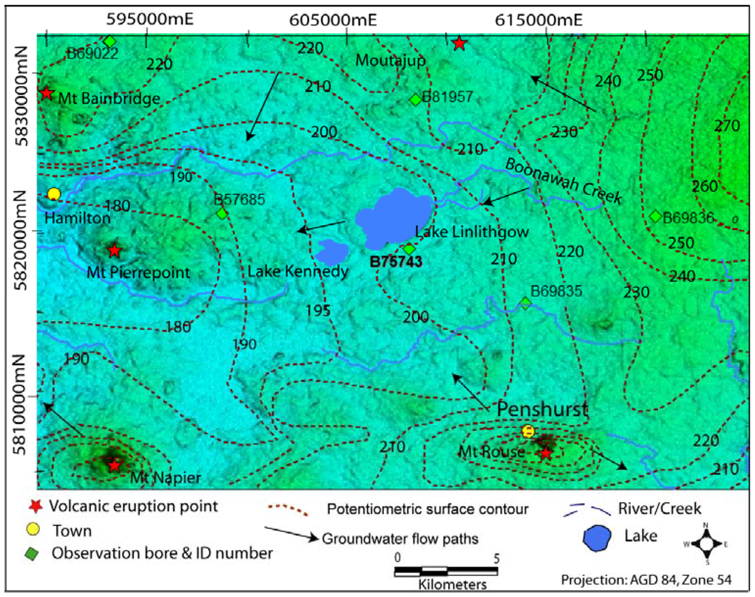
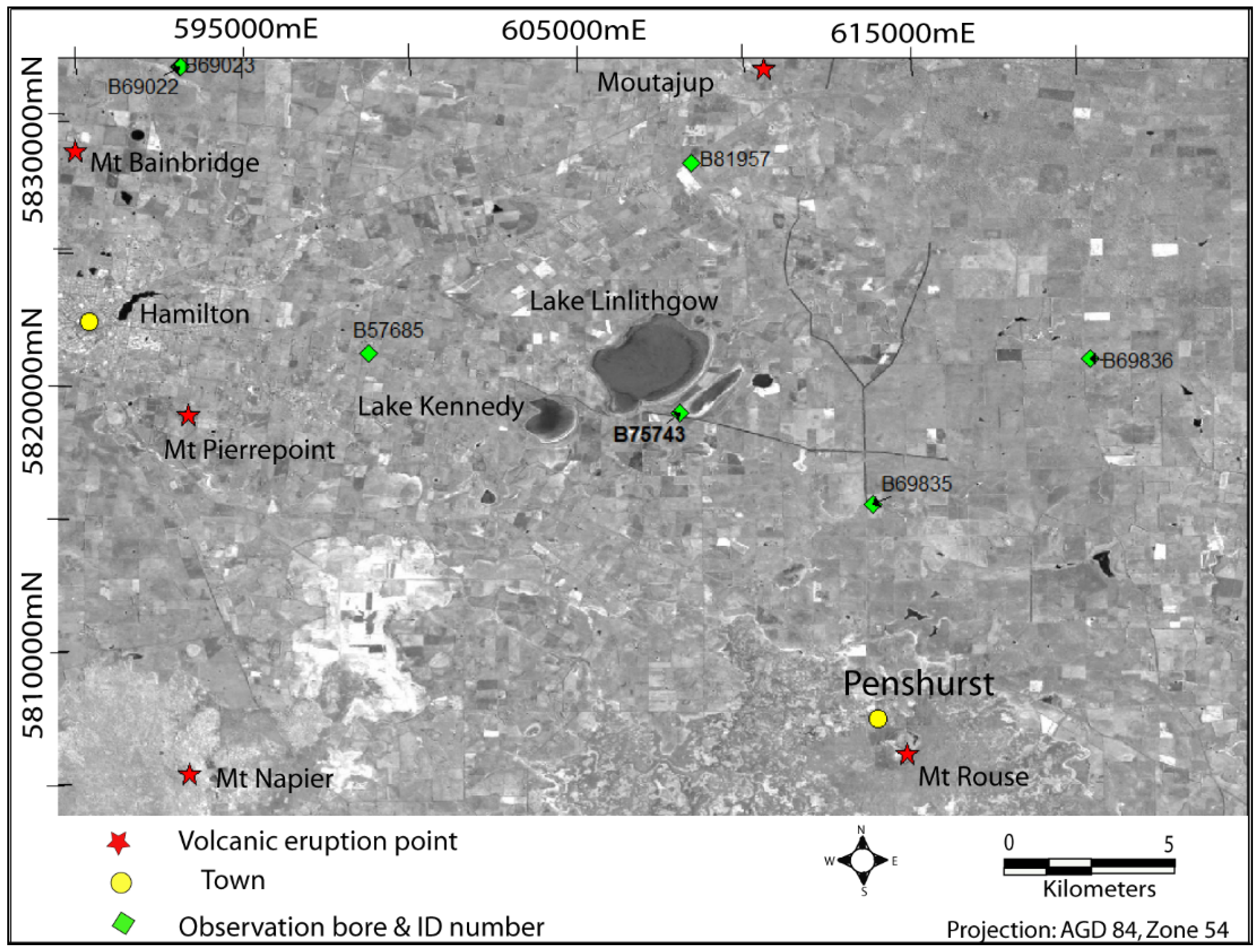
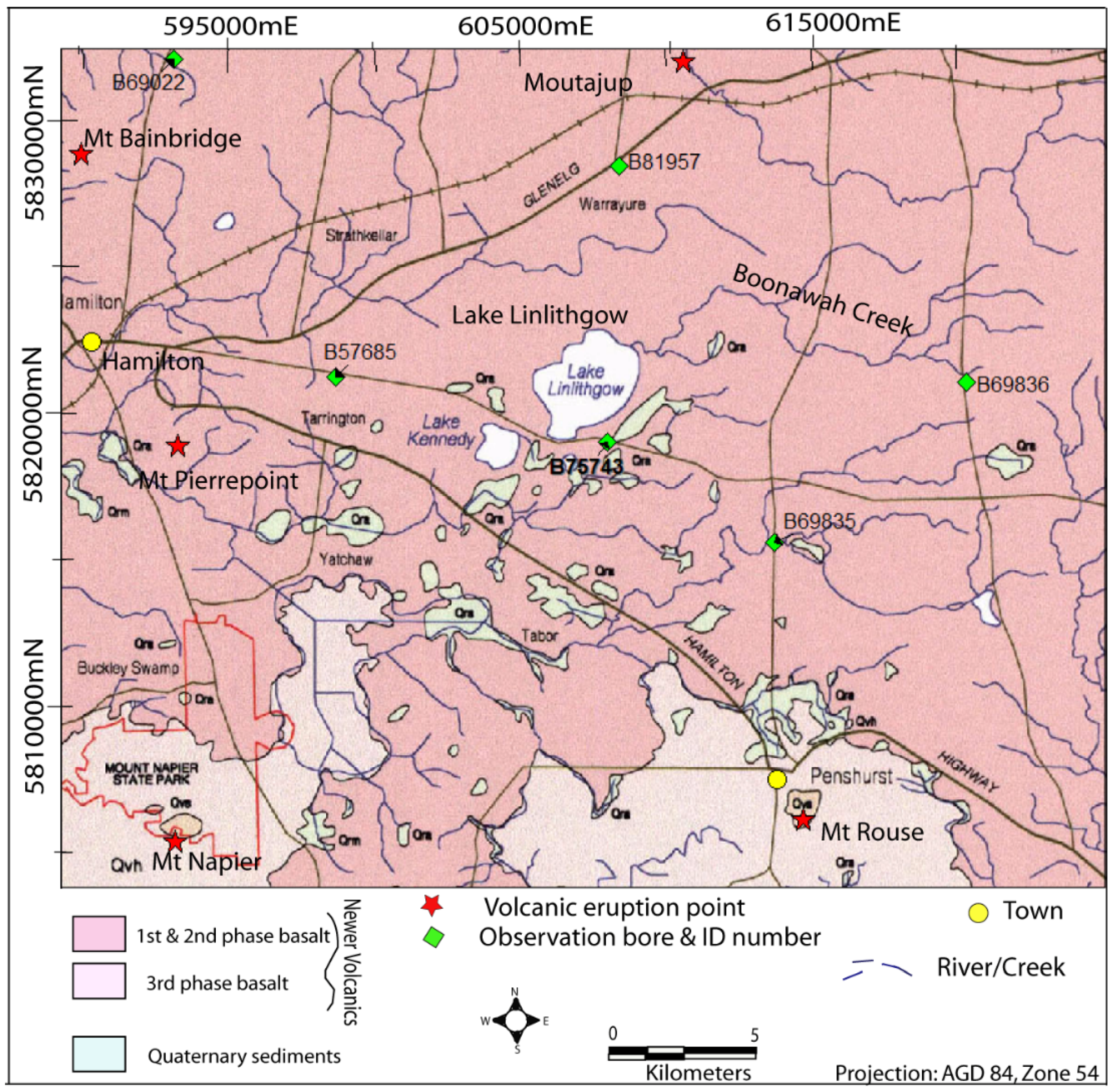
2. Study Area
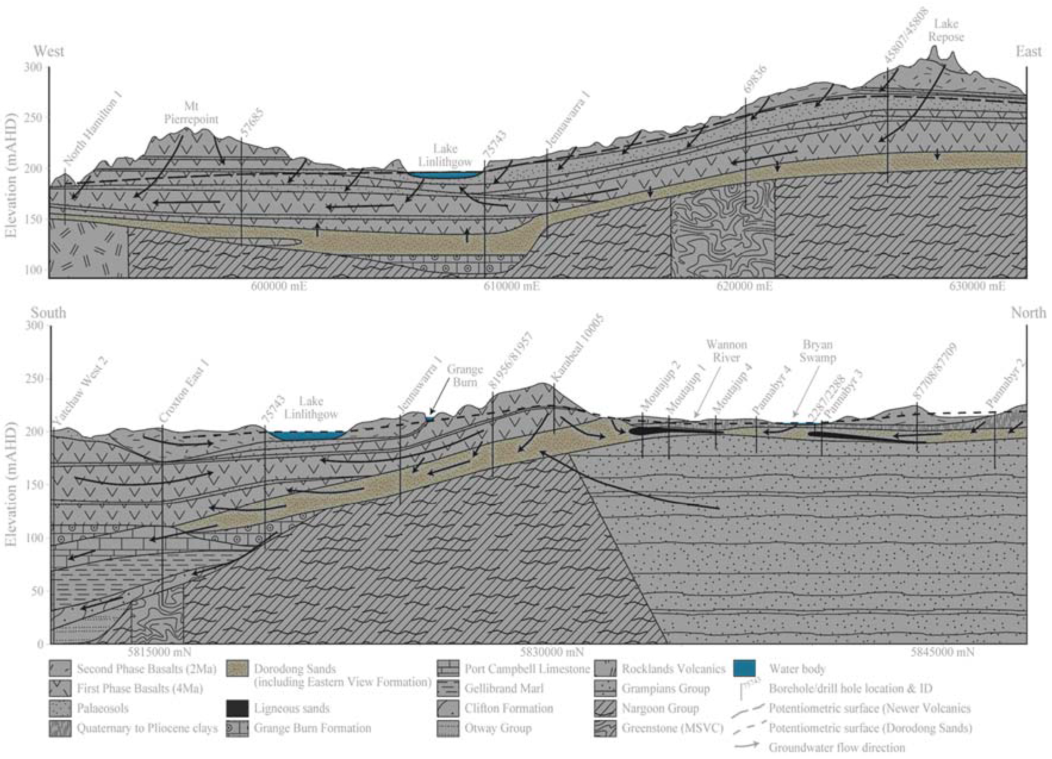
2.1. Hydrology
2.2. Geology
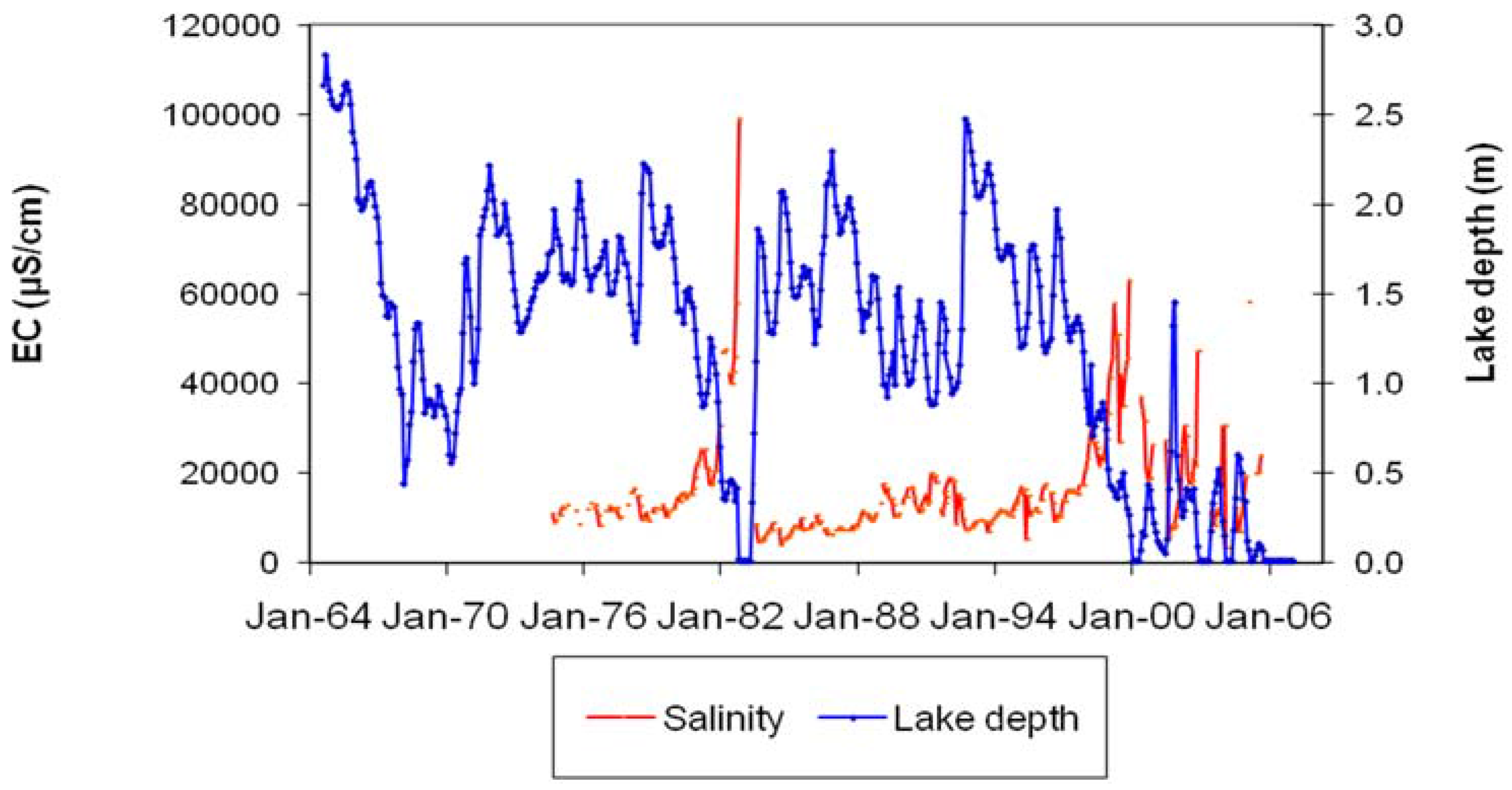
2.3. Lake Hydrology
3. Methodology
3.1. Water Balance Model
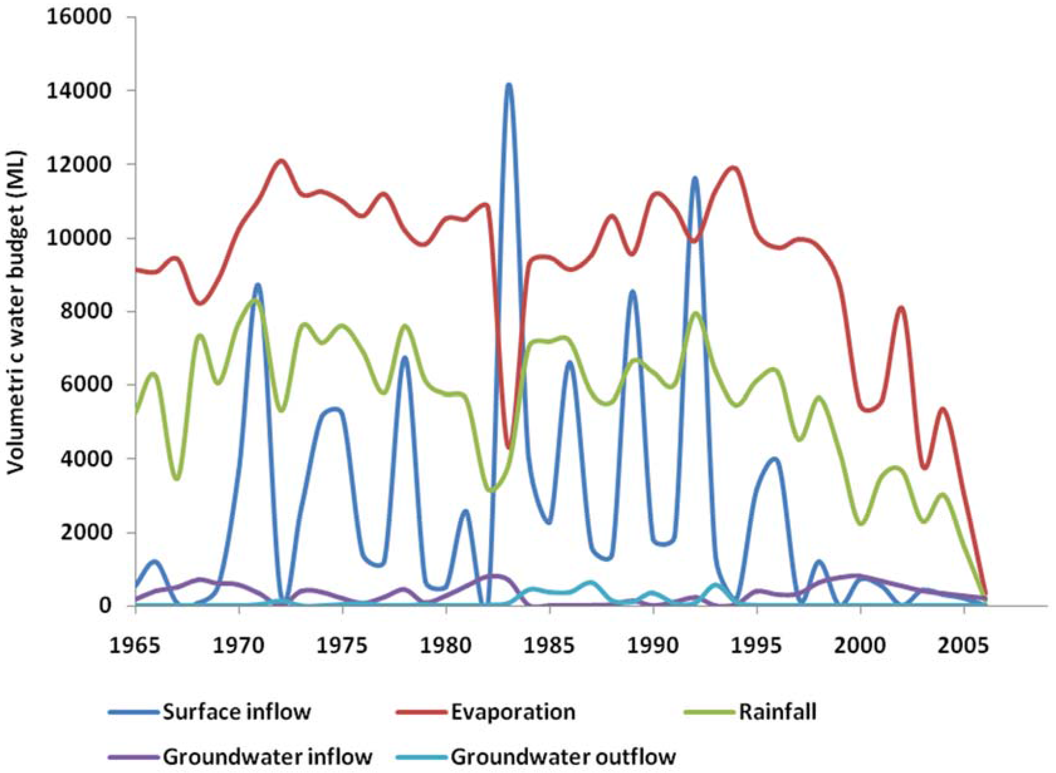
3.2. Lake Water Budget and Model Parameters
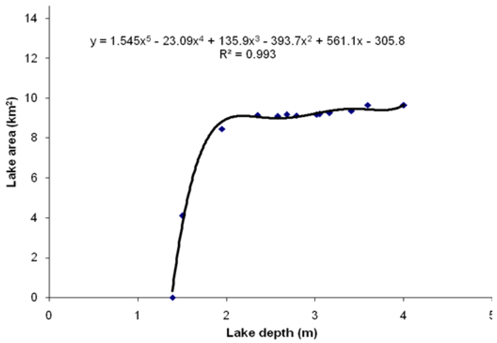
3.2.1. Lake Storage
3.2.2. Precipitation on Lake
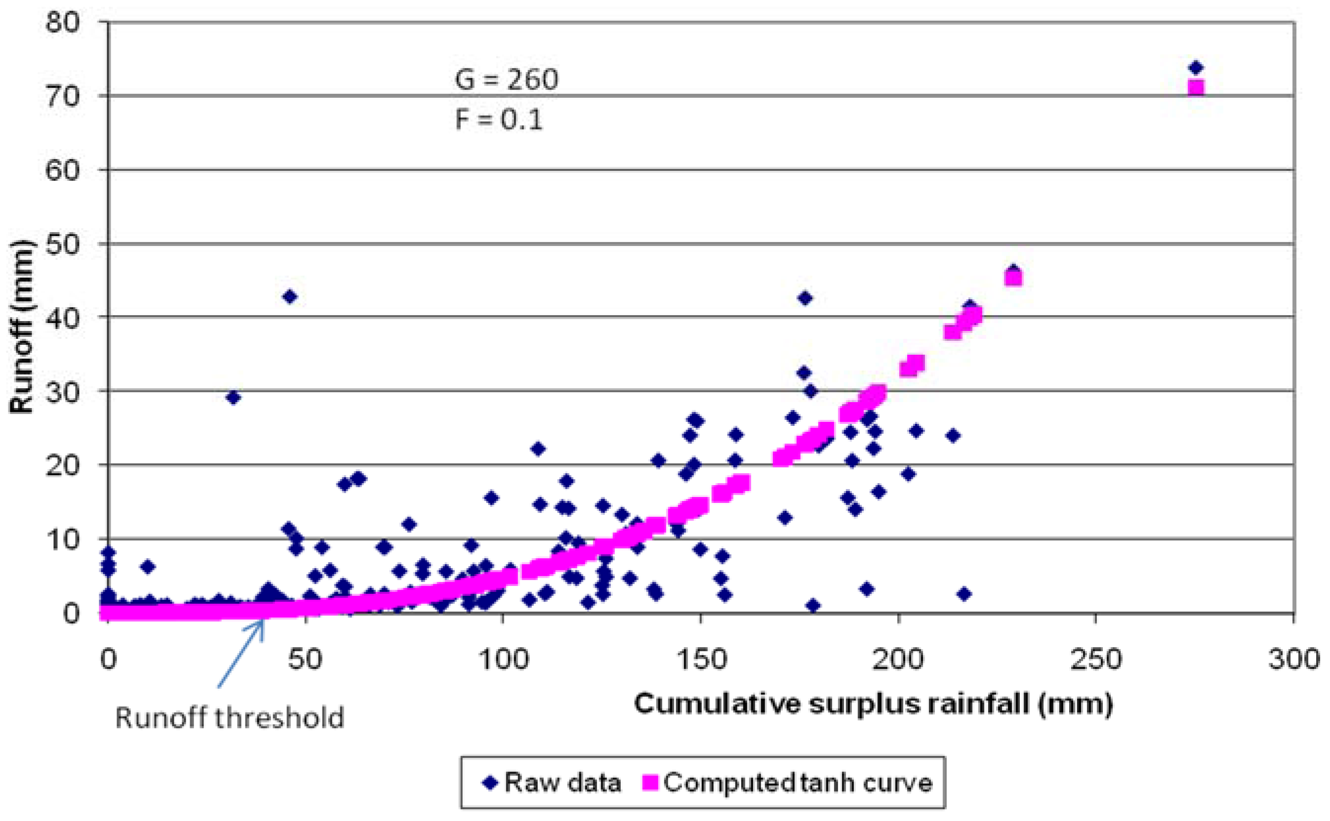
3.2.3. Surface Flow to the Lake
3.2.4. Outflow from the Lake
3.2.5. Groundwater Inflow and Outflow Estimation
4. Results and Discussion
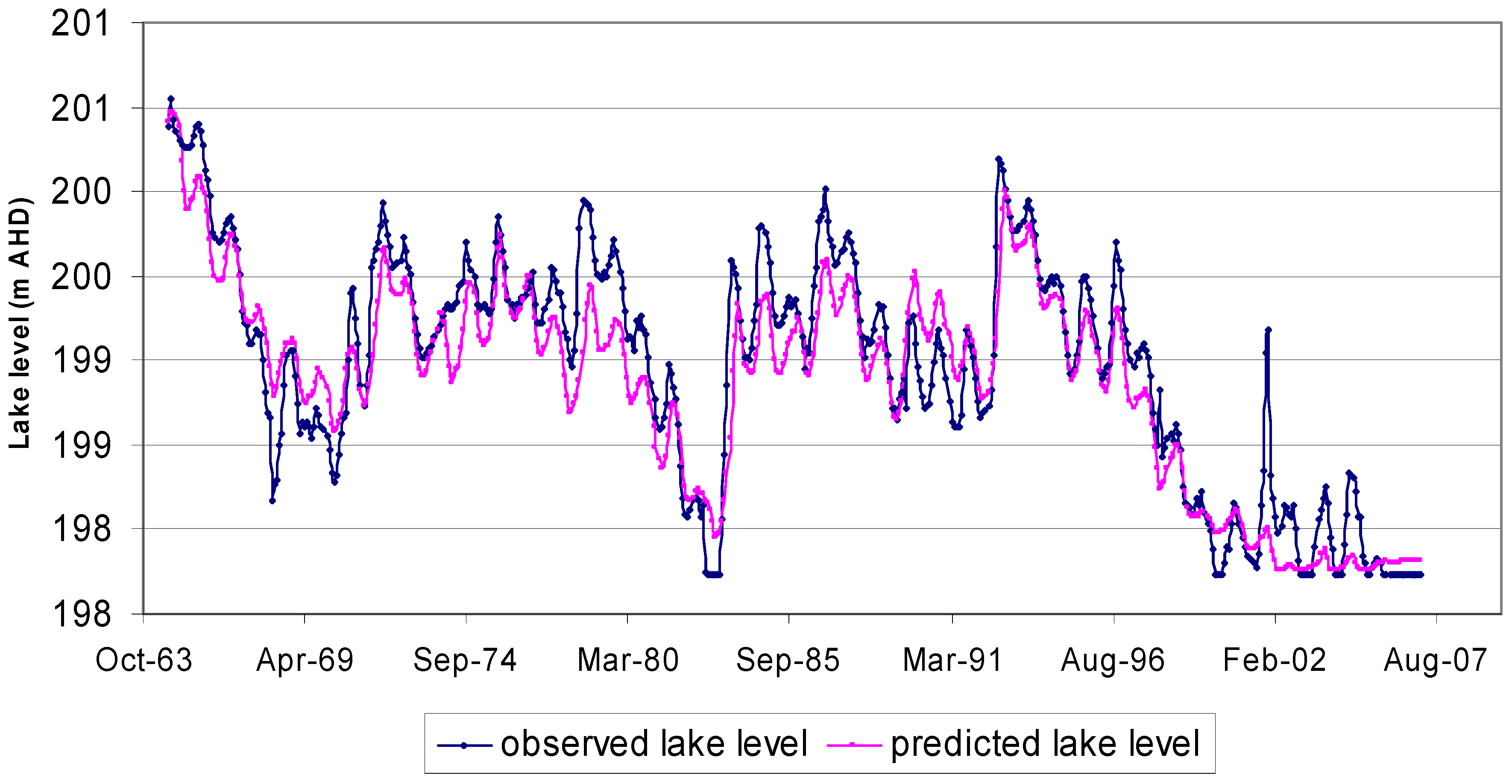
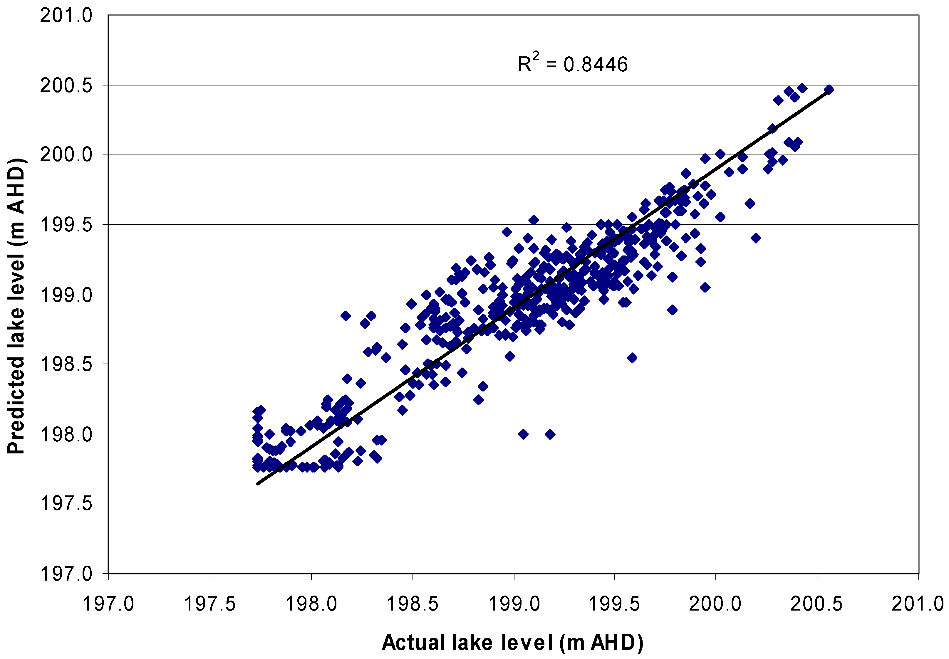
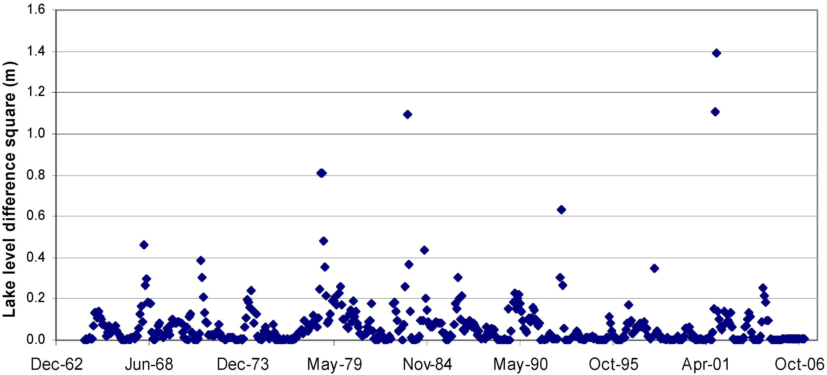
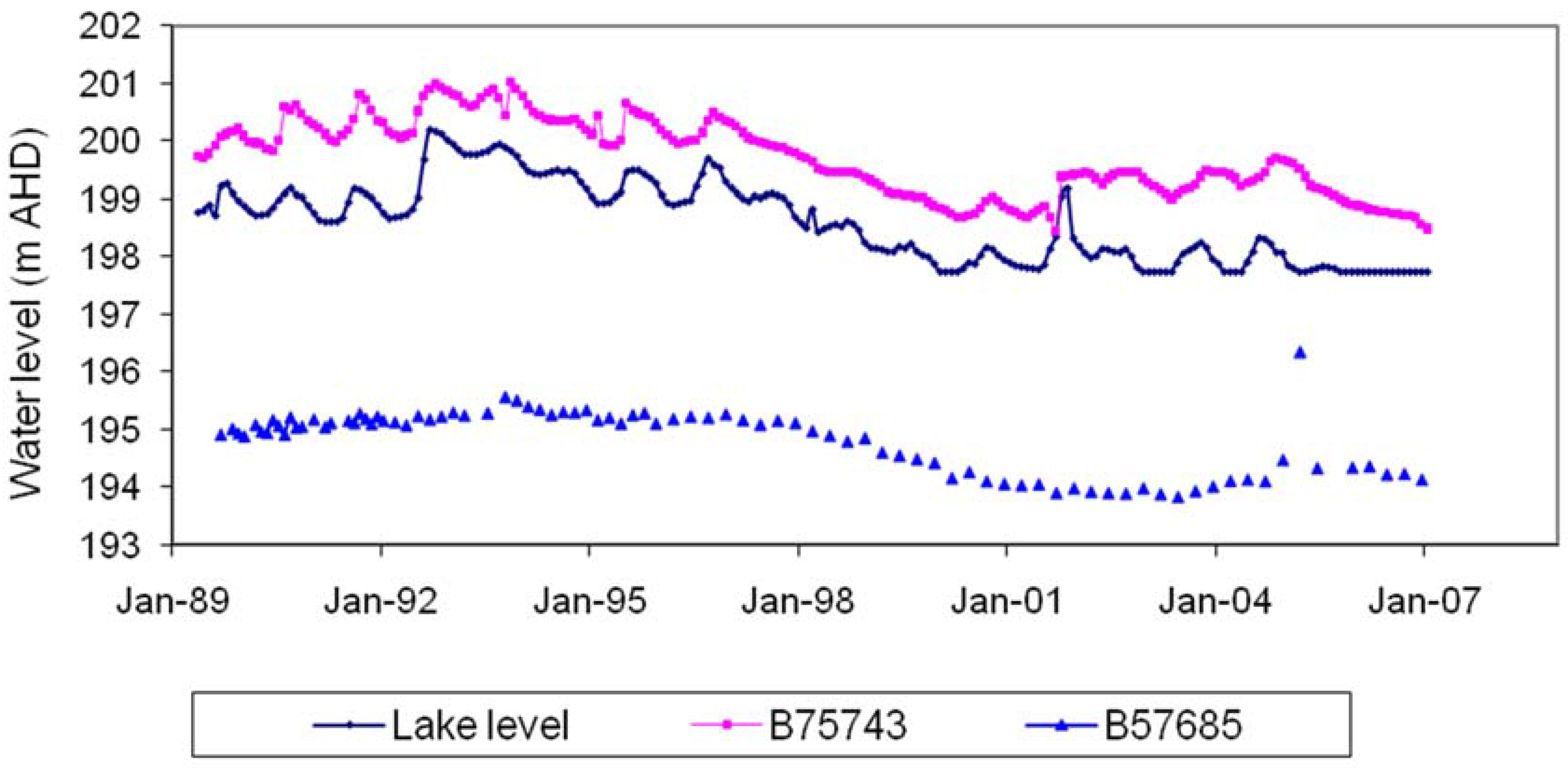
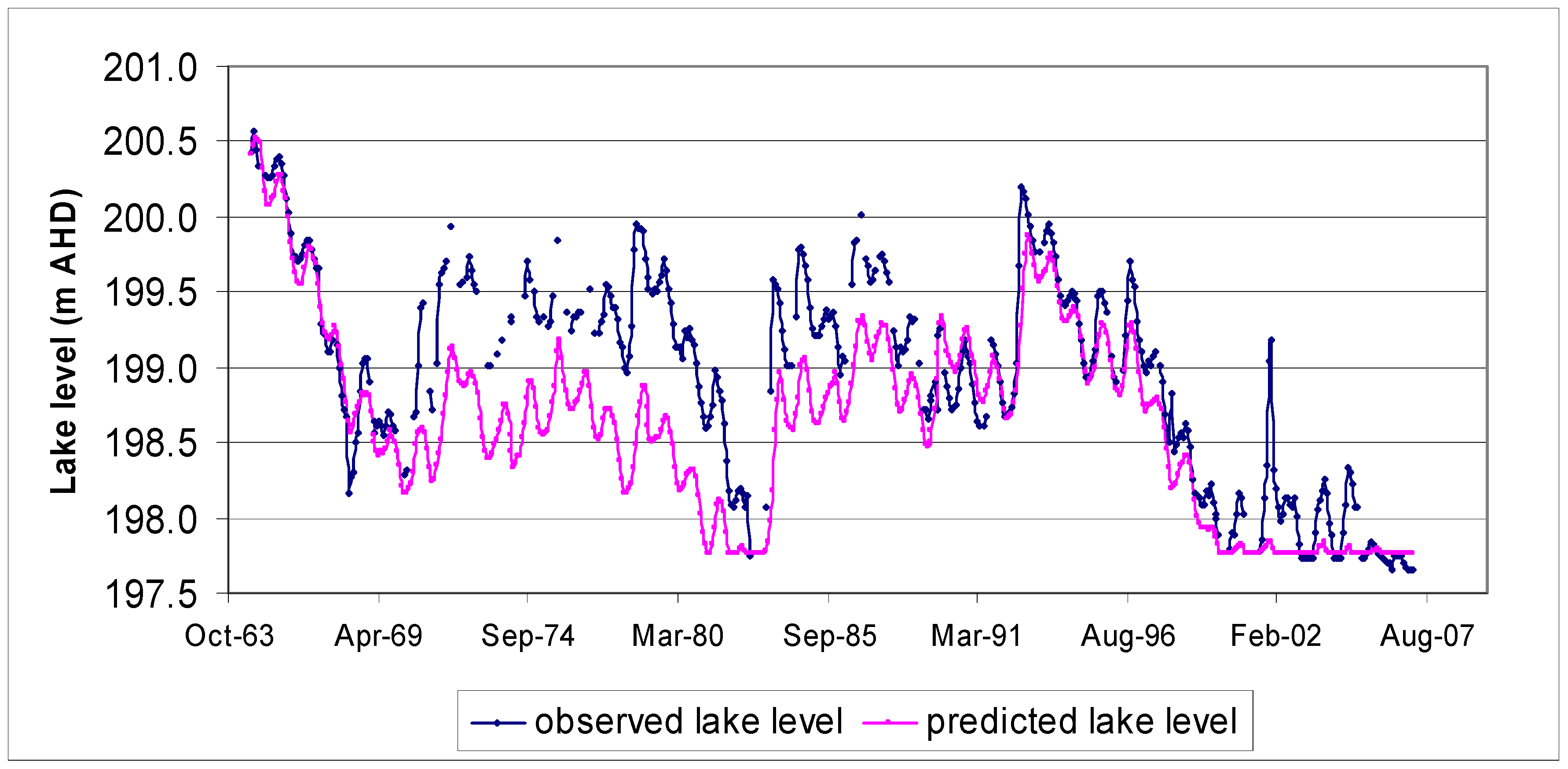
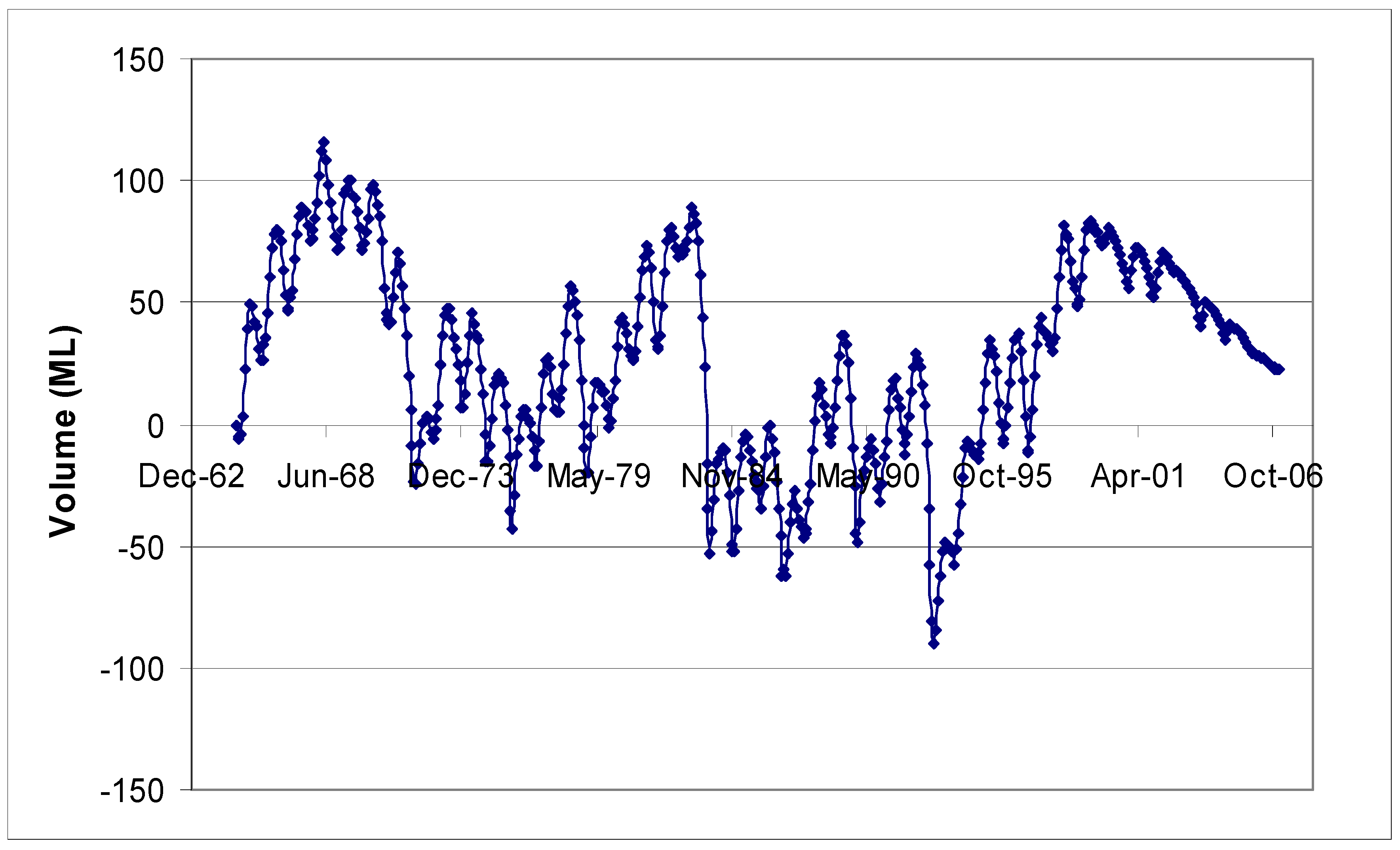
4.1. Lake Water Levels
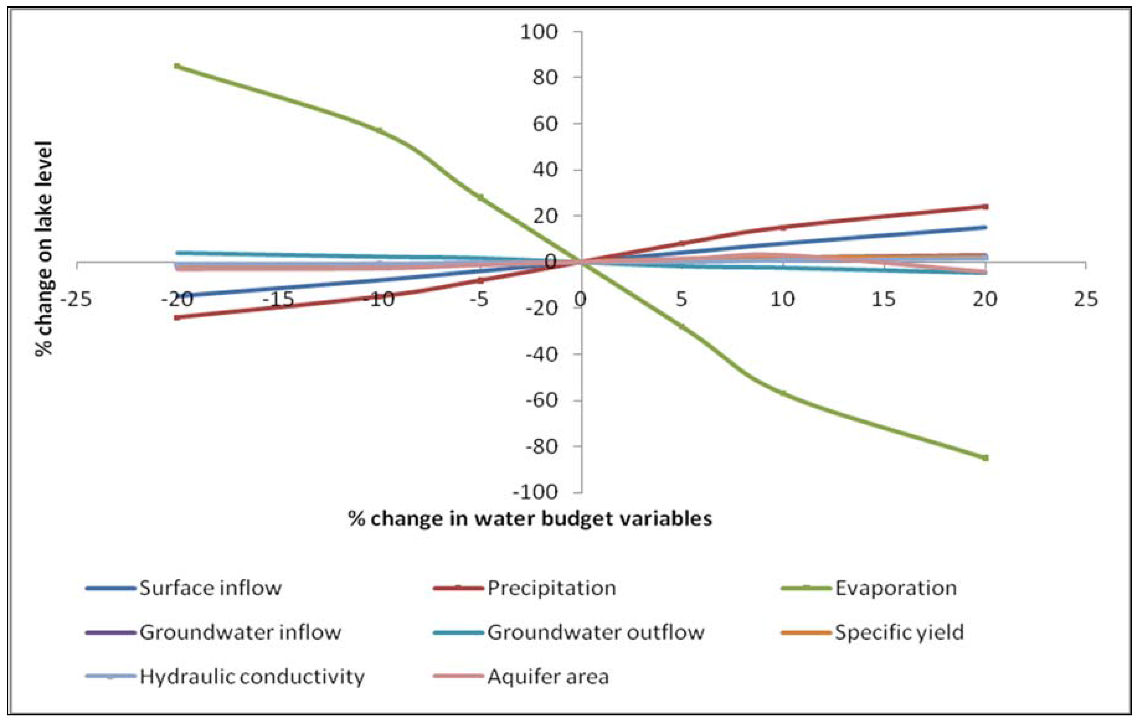
4.2. Water Budget Errors and Sensitivity Analysis
4.3. Interpretation
5. Conclusions
Acknowledgments
Author Contributions
Conflicts of Interest
References
- Dausman, A.M.; Doherty, J.; Langevin, C.D.; Dixon, J. Hypothesis testing of buoyant plume migration using a highly parameterized variable-density groundwater model. Hydrogeol. J. 2010, 18, 147–160. [Google Scholar] [CrossRef]
- Edelman, J.H. Groundwater Hydraulics of Extensive Aquifers (No. 13); International Livestock Research Institute, Wageningen University: Wageningen, The Netherlands, 1983. [Google Scholar]
- Yihdego, Y.; Drury, L. Mine water supply assessment and evaluation of the system response to the designed demand in a desert region, central Saudi Arabia. Environ. Monit. Assess. J. 2016, 188, 619. [Google Scholar] [CrossRef] [PubMed]
- Yihdego, Y.; Drury, L. Mine dewatering and impact assessment: Case of Gulf region. Environ. Monit. Assess. J. 2016, 188, 634. [Google Scholar] [CrossRef] [PubMed]
- Yihdego, Y.; Paffard, A. Predicting open mine inflow and recovery depth in the Durvuljin soum, Zavkhan Province, Mongolia. In Mine Water and the Environment; Springer: Berlin/Heidelberg, Germany, 2016; pp. 1–10. [Google Scholar]
- Yihdego, Y.; Paffard, A. Hydro-engineering solution for a sustainable groundwater management at a cross border region: Case of Lake Nyasa/Malawi basin, Tanzania. Int. J. Geo-Eng. 2016, 7, 23. [Google Scholar] [CrossRef]
- Christensen, S.; Doherty, J. Predictive error dependencies when using pilot points and singular value decomposition in groundwater model calibration. Adv. Water Resour. 2008, 31, 674–700. [Google Scholar] [CrossRef]
- Tonkin, M.; Doherty, J. Calibration-constrained Monte Carlo analysis of highly-parameterized models using subspace techniques. Water Resour. Res. 2008, 45, 12. [Google Scholar] [CrossRef]
- Yihdego, Y.; Webb, J.A. Hydrogeological constraints on the hydrology of Lake Burrumbeet, southwestern Victoria, Australia. In 21st VUEESC Conference, Victorian Universities Earth and Environmental Sciences Conference; Hagerty, S.H., McKenzie, D.S., Yihdego, Y., Eds.; Abstracts No 88, 12; Geological Society of Australia: Sydney, Australia, 2007. [Google Scholar]
- Yihdego, Y. Three Dimensional Groundwater Model of the Aquifer around Lake Naivasha Area, Kenya. Master’s Thesis, Department of Water Resources, ITC, University of Twente, Enschede, The Netherlands, March 2005. [Google Scholar]
- Yihdego, Y.; Webb, J.A. Characterizing groundwater dynamics in Western Victoria, Australia using Menyanthes software. In Proceedings of the 10th Australasian Environmental Isotope Conference and 3rd Australasian Hydrogeology Research Conference, Perth, Australia, 1–3 December 2009.
- Rosenberry, D.O.; Lewandowski, J.; Meinikmann, K.; Nützmann, G. Groundwater-the disregarded component in lake water and nutrient budgets. Part 1: Effects of groundwater on hydrology. Hydrol. Process. 2015, 29, 2895–2921. [Google Scholar] [CrossRef]
- Scibek, J.; Allen, D.M.; Cannon, A.J.; Whitfield, P.H. Groundwater–surface water interaction under scenarios of climate change using a high-resolution transient groundwater model. J. Hydrol. 2007, 333, 165–181. [Google Scholar] [CrossRef]
- Yihdego, Y.; Webb, J.A. Modeling of bore hydrographs to determine the impact of climate and land use change in a temperate subhumid region of southeastern Australia. Hydrogeol. J. 2011, 19, 877–887. [Google Scholar] [CrossRef]
- Yihdego, Y.; Webb, J.A.; Leahy, P. Response to Parker: Rebuttal: ENGE-D-13-00994R2 “Modelling of lake level under climate change conditions: Lake Purrumbete in south eastern Australia”. Environ. Earth Sci. J. 2016, 75, 1–4. [Google Scholar] [CrossRef]
- Yihdego, Y.; Webb, J.A. Assessment of wetland hydrological dynamics in a modified catchment basin: Case of Lake Buninjon, Victoria, Australia. Water Environ. Res. J. 2017, 89, 144–154. [Google Scholar] [CrossRef] [PubMed]
- Doherty, J.; Hunt, R.J. Response to comment on “Two statistics for evaluating parameter identifiability and error reduction”. J. Hydrol. 2010, 380, 489–496. [Google Scholar] [CrossRef]
- Doherty, J.; Johnston, J.M. Methodologies for calibration and predictive analysis of a watershed model. J. Am. Water Resour. Assoc. 2003, 39, 251–265. [Google Scholar] [CrossRef]
- Yihdego, Y. Drought and Pest Management Initiatives (Book chapter 11). In Handbook of Drought and Water Scarcity (HDWS): Vol. 3: Management of Drought and Water Scarcity; Eslamian, S., Eslamian, F.A., Eds.; Francis and Taylor, CRC Group: Burlington, MA, USA, 2016. [Google Scholar]
- Yihdego, Y. Drought and Groundwater Quality in Coastal Area (Book chapter 15). In Handbook of Drought and Water Scarcity (HDWS): Vol. 2: Environmental Impacts and Analysis of Drought and Water Scarcity; Eslamian, S., Eslamian, F.A., Eds.; Francis and Taylor, CRC Group: Burlington, MA, USA, 2016. [Google Scholar]
- Lewandowski, J.; Meinikmann, K.; Nützmann, G.; Rosenberry, D.O. Groundwater–the disregarded component in lake water and nutrient budgets. Part 2: Effects of groundwater on nutrients. Hydrol. Process. 2015, 29, 2922–2955. [Google Scholar] [CrossRef]
- Shaw, G.D.; White, E.S.; Gammons, C.H. Characterizing groundwater–lake interactions and its impact on lake water quality. J. Hydrol. 2013, 492, 69–78. [Google Scholar] [CrossRef]
- Yihdego, Y.; Al-Weshah, R. Hydrocarbon assessment and prediction due to the Gulf War oil disaster, North Kuwait. J. Water Environ. Res. 2016. [Google Scholar] [CrossRef]
- Yihdego, Y.; Al-Weshah, R. Gulf war contamination assessment for optimal monitoring and remediation cost –benefit analysis, Kuwait. Environ. Earth Sci. 2016, 75, 1–11. [Google Scholar] [CrossRef]
- Gallagher, M.R.; Doherty, J. Predictive error analysis for a water resource management model. J. Hydrol. 2007, 34, 513–533. [Google Scholar] [CrossRef]
- Hunt, R.J.; Doherty, J.; Tonkin, M.J. Are models too simple? Arguments for increased parameterization. Ground Water 2007, 45, 254–262. [Google Scholar] [CrossRef] [PubMed]
- Yihdego, Y.; Eslamian, S. Drought Management Initiatives and Objectives (Book chapter 1). In Handbook of Drought and Water Scarcity (HDWS): Vol. 3: Management of Drought and Water Scarcity; Eslamian, S., Eslamian, F.A., Eds.; Francis and Taylor, CRC Group: Burlington, MA, USA, 2016; p. 41. [Google Scholar]
- Shaw, G.D.; Mitchell, K.L.; Gammons, C.H. Estimating groundwater inflow and leakage outflow for an intermontane lake with a structurally complex geology: Georgetown Lake in Montana, USA. Hydrogeol. J. 2016, 1–15. [Google Scholar] [CrossRef]
- Skahill, B.; Doherty, J. Efficient accommodation of local minima in watershed model calibration. J. Hydrol. 2006, 329, 122–139. [Google Scholar] [CrossRef]
- Tonkin, M.; Doherty, J. A hybrid regularised inversion methodology for highly parameterized models. Water Resour. Res. 2005, 41, W10412. [Google Scholar] [CrossRef]
- Yihdego, Y. Data visualization tool as a framework for groundwater flow and transport models. In Proceedings of the International Conference on “MODFLOW and more 2013”, Translating Science into Practice; Integrated Groundwater Modelling Centre (IGWMC), Colorado School of Mines, University: Golden, CO, USA, 2013. [Google Scholar]
- Yihdego, Y.; Webb, J.A. Modelling of seasonal and long-term trends in lake salinity in south-western Victoria, Australia. J. Environ. Manag. 2012, 112, 149–159. [Google Scholar] [CrossRef] [PubMed]
- Gallagher, M.R.; Doherty, J. Parameter estimation and uncertainty analysis for a watershed model. Environ. Model. Softw. 2006, 22, 1000–1020. [Google Scholar] [CrossRef]
- Lohman, S.W. Ground-Water Hydraulics; US Government Printing Office: Washington, DC, USA, 1972; p. 70.
- Lewis, M.A.; Cheney, C.S.; ÓDochartaigh, B.E. Guide to Permeability Indices; CR/06/160N; British Geological Survey, Natural Environmental Council: London, UK, 2006. [Google Scholar]
- Post, V.; Kooi, H.; Simmons, C. Using hydraulic head measurements in variable-density ground water flow analyses. Ground Water 2007, 45, 664–671. [Google Scholar] [CrossRef] [PubMed]
- Jakovovic, D.; Werner, A.D.; de Louw, P.G.; Post, V.E.; Morgan, L.K. Saltwater upcoming zone of influence. Adv. Water Resour. 2016, 94, 75–86. [Google Scholar] [CrossRef]
- Yihdego, Y.; Reta, G.; Becht, R. Hydrological analysis as a technical tool to support strategic and economic development: Case of Lake Navaisha, Kenya. Water Environ. J. 2016, 30, 40–48. [Google Scholar] [CrossRef]
- Yihdego, Y.; Reta, G.; Becht, R. Human impact assessment through a transient numerical modelling on The UNESCO World Heritage Site, Lake Navaisha, Kenya. Environ. Earth Sci. 2017, 76, 9. [Google Scholar] [CrossRef]
- Yihdego, Y.; Webb, J.A. Validation of a model with climatic and flow scenario analysis: Case of Lake Burrumbeet in Southeastern Australia. Environ. Monit. Assess. 2016, 188, 1–14. [Google Scholar] [CrossRef] [PubMed]
- Jones, R.N.; McMahon, T.A.; Bowler, J.M. Modelling historical lake levels and recent climate change at three closed lakes, Western Victoria, Australia (c.1840–1990). J. Hydrol. 2001, 246, 159–180. [Google Scholar] [CrossRef]
- Yihdego, Y.; Webb, J.A. An empirical water budget model as a tool to identify the impact of land-use change on stream flow in southeastern Australia. Water Resour. Manag. 2012, 27, 4941–4958. [Google Scholar] [CrossRef]
- James, S.C.; Doherty, J.; Eddebarh, A.A. Post-calibration uncertainty analysis: Yucca Mountain, Nevada, USA. Ground Water 2009, 47, 851–869. [Google Scholar] [CrossRef] [PubMed]
- Tonkin, M.; Doherty, J.; Moore, C. Efficient nonlinear predictive error variance analysis for highly parameterized models. Water Resour. Res. 2007, 43, 7. [Google Scholar] [CrossRef]
- Doherty, J.; Skahill, B. An advanced regularization methodology for use in watershed model calibration. J. Hydrol. 2006, 327, 564–577. [Google Scholar] [CrossRef]
- Doherty, J. Groundwater model calibration using pilot points and regularization. Ground Water 2003, 41, 170–177. [Google Scholar] [CrossRef]
- Moore, C.; Doherty, J. The cost of uniqueness in groundwater model calibration. Adv. Water Resour. 2006, 29, 605–623. [Google Scholar] [CrossRef]
- Yihdego, Y.; Becht, R. Simulation of lake–aquifer interaction at Lake Navaisha, Kenya using a three-dimensional flow model with the high conductivity technique and a DEM with bathymetry. J. Hydrol. 2013, 503, 111–122. [Google Scholar] [CrossRef]
- Yihdego, Y.; Al-Weshah, R. Engineering and environmental remediation scenarios due to leakage from the Gulf War oil spill using 3-D numerical contaminant modellings. J. Appl. Water Sci. 2016. [Google Scholar] [CrossRef]
- Bennetts, D. Hydrology, Hydrogeology and Hydro-Geochemistry of Groundwater Flow Systems within the Hamilton Basalt Plains, Western Victoria, and Their Role in Dry Land Salinisation. Ph.D. Thesis, Department of Earth Sciences, La Trobe University, Melbourne, Australia, September 2005. [Google Scholar]
- Yihdego, Y.; Webb, J.A. Use of a conceptual hydrogeological model and a time variant water budget analysis to determine controls on salinity in Lake Burrumbeet in southeast Australia. Environ. Earth Sci. 2015, 73, 1587–1600. [Google Scholar] [CrossRef]
- Yihdego, Y.; Webb, J.A.; Leahy, P. Modelling of lake level under climate change conditions: Lake Purrumbete in southeastern Australia. Environ. Earth Sci. 2015, 73, 3855–3872. [Google Scholar] [CrossRef]
- Yihdego, Y.; Webb, J.A.; Leahy, P. Modelling water and salt balances in a deep, groundwater-throughflow lake—Lake Purrumbete, southeastern Australia. Hydrol. Sci. J. 2016, 61, 186–199. [Google Scholar] [CrossRef]
- Yihdego, Y. Modelling of Lake Level and Salinity for Lake Purrumbete in Western Victoria, Australia; A Co-Operative Research Project between La Trobe University and EPA Victoria; EPA Victoria: Melbourne, Australia, 2010. [Google Scholar]
- Yihdego, Y. Modelling Bore and Stream Hydrograph and Lake Level in Relation to Climate and Land Use Change in Southwestern Victoria, Australia. Ph.D. Thesis, Faculty of Science, Technology and Engineering, Melbourne, La Trobe University, Melbourne, Australia, May 2010. [Google Scholar]
- Yihdego, Y.; Webb, J.A. Characterizing groundwater dynamics using Transfer Function-Noise and auto-regressive modelling in Western Victoria, Australia. In Proceedings of the 5th IASME/WSEAS International Conference on Water Resources, Hydraulics and Hydrology (WHH ’10), Cambridge, UK, 23–25 February 2010.
- Yihdego, Y.; Al-Weshah, R. Assessment and prediction of saline sea water transport in groundwater using using 3-D numerical modelling. Environ. Process. J. 2016. [Google Scholar] [CrossRef]
- Winter, T.C. Effects of water table configuration on seepage through lakebeds. Limnol. Oceanogr. 1981, 26, 925–934. [Google Scholar] [CrossRef]
- Yihdego, Y. Evaluation of Flow Reduction due to Hydraulic Barrier Engineering Structure: Case of Urban Area Flood, Contamination and Pollution Risk Assessment. J. Geotech. Geol. Eng. 2016, 34, 1643–1654. [Google Scholar] [CrossRef]
- Al-Weshah, R.; Yihdego, Y. Modelling of Strategically Vital Fresh Water Aquifers, Kuwait. Environ. Earth Sci. 2016, 75, 1315. [Google Scholar] [CrossRef]
- Yihdego, Y.; Danis, C.; Paffard, A. 3-D numerical groundwater flow simulation for geological discontinuities in the Unkheltseg Basin, Mongolia. Environ. Earth Sci. J. 2015, 73, 4119–4133. [Google Scholar] [CrossRef]
- Yihdego, Y.; Webb, J.A. Characterizing groundwater dynamics in Western Victoria, Australia using Menyanthes software. In Proceedings of the 10th Australasian Environmental Isotope Conference and 3rd Australasian Hydrogeology Research Conference, Perth, Australia, 1–3 December 2009.
- Yihdego, Y.; Webb, J.A. Modelling of Seasonal and Long-term Trends in Lake Salinity in Southwestern Victoria, Australia. J. Environ. Manag. 2012, 112, 149–159. [Google Scholar]
- Yihdego, Y. Engineering and enviro-management value of radius of influence estimate from mining excavation. J. Appl. Water Eng. Res. 2017. [Google Scholar] [CrossRef]


| Evaporation (%) | Groundwater Outflow (%) | Precipitation (%) | Surface Inflow (%) | Groundwater Inflow (%) |
|---|---|---|---|---|
| 54 | 0.1 | 37 | 8 | 1 |
© 2017 by the authors; licensee MDPI, Basel, Switzerland. This article is an open access article distributed under the terms and conditions of the Creative Commons Attribution (CC BY) license (http://creativecommons.org/licenses/by/4.0/).
Share and Cite
Yihdego, Y.; Webb, J.A.; Vaheddoost, B. Highlighting the Role of Groundwater in Lake– Aquifer Interaction to Reduce Vulnerability and Enhance Resilience to Climate Change. Hydrology 2017, 4, 10. https://doi.org/10.3390/hydrology4010010
Yihdego Y, Webb JA, Vaheddoost B. Highlighting the Role of Groundwater in Lake– Aquifer Interaction to Reduce Vulnerability and Enhance Resilience to Climate Change. Hydrology. 2017; 4(1):10. https://doi.org/10.3390/hydrology4010010
Chicago/Turabian StyleYihdego, Yohannes, John A Webb, and Babak Vaheddoost. 2017. "Highlighting the Role of Groundwater in Lake– Aquifer Interaction to Reduce Vulnerability and Enhance Resilience to Climate Change" Hydrology 4, no. 1: 10. https://doi.org/10.3390/hydrology4010010